Eigenvalues and eigenvectors of heavy-tailed sample covariance matrices with general growth rates: the iid case

Abstract.

In this paper we study the joint distributional convergence of the largest eigenvalues of the sample covariance matrix of a $p$-dimensional time series with iid entries when $p$ converges to infinity together with the sample size $n$. We consider only heavy-tailed time series in the sense that the entries satisfy some regular variation condition which ensures that their fourth moment is infinite. In this case, Soshnikov [31, 32] and Auffinger et al. [2] proved the weak convergence of the point processes of the normalized eigenvalues of the sample covariance matrix towards an inhomogeneous Poisson process which implies in turn that the largest eigenvalue converges in distribution to a Fréchet distributed random variable. They proved these results under the assumption that $p$ and $n$ are proportional to each other. In this paper we show that the aforementioned results remain valid if $p$ grows at any polynomial rate. The proofs are different from those in [2, 31, 32]; we employ large deviation techniques to achieve them. The proofs reveal that only the diagonal of the sample covariance matrix is relevant for the asymptotic behavior of the largest eigenvalues and the corresponding eigenvectors which are close to the canonical basis vectors. We also discuss extensions of the results to sample autocovariance matrices.

1. Introduction

In recent years we have seen a vast increase in the number and sizes of data sets. Science (meteorology, telecommunications, genomics, …), society (social networks, finance, military and civil intelligence, …) and industry need to extract valuable information from high-dimensional data sets which are often too large or complex to be processed by traditional means. In order to explore the structure of data one often studies the dependence via (sample) covariances and correlations. Often dimension reduction techniques facilitate further analyzes of large data matrices. For example, principal component analysis (PCA) transforms the data linearly such that only a few of the resulting vectors contain most of the variation in the data. These principal component vectors are the eigenvectors associated with the largest eigenvalues of the sample covariance matrix.

The aim of this paper is to investigate the asymptotic properties of the largest eigenvalues and their corresponding eigenvectors for sample covariance matrices of high-dimensional heavy-tailed time series with iid entries. Special emphasis is given to the case when the dimension $p$ and the sample size $n$ tend to infinity simultaneously, not necessarily at the same rate.

Throughout we consider the $p\times n$ data matrix

$${\mathbf{Z}}={\mathbf{Z}}_{n}=\big{(}Z_{it}\big{)}_{i=1,\ldots,p;t=1,\ldots,n}\,$$

A column of ${\mathbf{Z}}$ represents an observation of a $p$-dimensional time series. We assume that the entries $Z_{it}$ are real-valued, independent and identically distributed (iid), unless stated otherwise. We write $Z$ for a generic element and assume $\mathbb{E}[Z]=0$ and $\mathbb{E}[Z^{2}]=1$ if the first and second moments of $Z$ are finite, respectively. We are interested in limit theory for the eigenvalues $\lambda_{1},\ldots,\lambda_{p}$ of the sample covariance matrix ${\mathbf{Z}}{\mathbf{Z}}^{\prime}$ and their ordered values

$$\lambda_{(1)}\geq\cdots\geq\lambda_{(p)}\,.$$ (1.1)

In this notation we suppress the dependence of $(\lambda_{i})$ on $n$. We will only discuss the case when $p\to\infty$; for the finite $p$ case we refer to [1, 26].

1.1. The light-tailed case

In random matrix theory a lot of attention has been given to the empirical spectral distribution function of the sequence $(n^{-1}{\mathbf{Z}}{\mathbf{Z}}^{\prime})$:

$$F_{n^{-1}{\mathbf{Z}}{\mathbf{Z}}^{\prime}}(x)=\frac{1}{p}\;\#\{1\leq j\leq p:n^{-1}\lambda_{j}\leq x\},\qquad x\geq 0\,,\quad n\geq 1.$$

In the literature convergence results for $(F_{n^{-1}{\mathbf{Z}}{\mathbf{Z}}^{\prime}})$ are established under the assumption that $p$ and $n$ grow at the same rate:

$$\dfrac{p}{n}\to\gamma\qquad\mbox{for some $\gamma\in(0,\infty)$.}$$ (1.2)

Suppose that the iid entries $Z_{it}$ have mean $0$ and variance $1$. If (1.2) holds then, with probability one, $(F_{n^{-1}{\mathbf{Z}}{\mathbf{Z}}^{\prime}})$ converges to the Marčenko–Pastur law with absolutely continuous part given by the density,

$$f_{\gamma}(x)=\left\{\begin{array}[]{cc}\frac{1}{2\pi x\gamma}\sqrt{(b-x)(x-a)}\,,&\mbox{if }a\leq x\leq b,\\ 0\,,&\mbox{otherwise,}\end{array}\right.$$ (1.5)

where $a=(1-\sqrt{\gamma})^{2}$ and $b=(1+\sqrt{\gamma})^{2}$. For $\gamma>1$ the Marčenko–Pastur law has an additional point mass $1-1/\gamma$ at the origin; see Bai and Silverstein [3, Chapter 3]. This mass is intuitively explained by the fact that, with probability $1$, $\min(p,n)$ eigenvalues $\lambda_{i}$ are non-zero. When $n=(1/\gamma)\;p$ and $\gamma>1$ the fraction of non-zero eigenvalues is $1/\gamma$ while the fraction of zero eigenvalues is $1-1/\gamma$.

The moment condition $\mathbb{E}[Z^{2}]<\infty$ is crucial for deriving the Marčenko–Pastur limit law. When studying the largest eigenvalues of the sample covariance matrix ${\mathbf{Z}}{\mathbf{Z}}^{\prime}$ the moment condition $\mathbb{E}[Z^{4}]<\infty$ plays a similarly important role; we assume it in the remainder of this subsection. If (1.2) holds and the iid entries $Z_{it}$ have zero mean and unit variance, Geman [19] showed that

$$\dfrac{\lambda_{(1)}}{n}\stackrel{{\scriptstyle\rm a.s.}}{{\rightarrow}}\big{(}1+\sqrt{\gamma}\big{)}^{2}\,,\qquad n\to\infty\,.$$ (1.6)

This means that $\lambda_{(1)}/n$ converges to the right endpoint of the Marčenko–Pastur law in (1.5). Johnstone [23] complemented this strong law of large numbers by the corresponding central limit theorem in the special case of iid standard normal entries:

$$\frac{\lambda_{(1)}-\mu_{n,p}}{\sigma_{n,p}}\stackrel{{\scriptstyle d}}{{\rightarrow}}\xi,$$ (1.7)

where the limiting random variable has a Tracy–Widom distribution of order 1 and the centering and scaling constants are

$$\mu_{n,p}=(\sqrt{n-1}+\sqrt{p})^{2},\quad\sigma_{n,p}=(\sqrt{n-1}+\sqrt{p})\Big{(}\frac{1}{\sqrt{n-1}}+\frac{1}{\sqrt{p}}\Big{)}^{1/3}\,;$$

see Tracy and Widom [35] for details. Ma [25] showed Berry–Esseen-type bounds for (1.7).

Asymptotic theory for the largest eigenvalues of sample covariance matrices with non-Gaussian entries is more complicated; pioneering work is due to Johansson [22]. Johnstone’s result was extended to matrices ${\mathbf{Z}}$ with iid non-Gaussian entries by Tao and Vu [33, Theorem 1.16], assuming that the first four moments of $Z$ match those of the normal distribution. Tao and Vu’s result is a consequence of the so-called Four Moment Theorem which describes the insensitivity of the eigenvalues with respect to changes in the distribution of the entries. To some extent (modulo the strong moment matching conditions) it shows the universality of Johnstone’s limit result (1.7).

In the light-tailed case little is known when $p$ and $n$ grow at different rates, i.e., $\lim p/n\in\{0,\infty\}$. Notable exceptions are El Karoui [16] who proved that Johnstone’s result (assuming iid standard normal entries) remains valid when $p/n\to 0$ or $n/p\to\infty$, and Péché [28] who showed universality results for the largest eigenvalues of some sample covariance matrices with non-Gaussian entries.

1.2. The heavy-tailed case

Distributions of which certain moments cease to exist are often called heavy-tailed. So far we reviewed theoretical results where the data matrix ${\mathbf{Z}}$ was “light-tailed” in the following sense: for the distributional convergence of the empirical spectral distribution and the largest eigenvalue of the sample covariance matrix towards the Marčenko–Pastur and Tracy-Widom distributions, respectively, we required finite second/fourth moments of the entries.

The behavior of the largest eigenvalue $\lambda_{(1)}$ changes dramatically when $\mathbb{E}[Z^{4}]=\infty$. Bai and Silverstein [4] proved for an $n\times n$ matrix ${\mathbf{Z}}$ with iid centered entries that

$$\limsup_{n\to\infty}\dfrac{\lambda_{(1)}}{n}=\infty\qquad{\rm a.s.}$$ (1.8)

This is in stark contrast to Geman’s result (1.6).

Following classical limit theory for partial sum processes and maxima, we require more than an infinite fourth moment. We assume a regular variation condition on the tail of $Z$:

$$\mathbb{P}(Z>x)\sim p_{+}\,\dfrac{L(x)}{x^{\alpha}}\qquad\mbox{and}\qquad\mathbb{P}(Z<-x)\sim p_{-}\,\dfrac{L(x)}{x^{\alpha}}\,,\qquad x\to\infty\,,$$ (1.9)

for some $\alpha\in(0,4)$, where $p_{\pm}$ are non-negative constants such that $p_{+}+p_{-}=1$ and $L$ is a slowly varying function. We will also refer to $Z$ as a regularly varying random variable, ${\mathbf{Z}}$ as a regularly varying matrix, etc. Here and in what follows, we normalize the eigenvalues $(\lambda_{i})$ by $(a_{np}^{2})$ where the sequence $(a_{k})$ is chosen such that

$$\mathbb{P}(|Z|>a_{k})\sim k^{-1}\,,\quad k\to\infty.$$

Standard theory for regularly varying functions (e.g. Bingham et al. [9], Feller [18]) yields that $a_{n}=n^{1/\alpha}\ell(n)$ where $\ell$ is a slowly varying function. Assuming (1.2) for $p$, the Potter bounds (see [9, p. 25]) yield for $\alpha\in(0,4)$ that

$$\frac{a_{np}^{2}}{n}\sim\frac{n^{4/\alpha}\gamma^{2/\alpha}\,\ell^{2}(n^{2}\gamma)}{n}\to\infty,\qquad n\to\infty\,,$$ (1.10)

i.e., the normalization $a_{np}^{2}$ is stronger than $n$.

The eigenvalues $(\lambda_{i})$ of a heavy-tailed matrix ${\mathbf{Z}}{\mathbf{Z}}^{\prime}$ were studied first by Soshnikov [31, 32]. He showed under (1.2) and (1.9) for $\alpha\in(0,2)$ that

$$\dfrac{\lambda_{(1)}}{a_{np}^{2}}\stackrel{{\scriptstyle d}}{{\rightarrow}}\zeta,\quad n\to\infty,$$ (1.11)

where $\zeta$ follows a Fréchet distribution with parameter $\alpha/2$:

$$\Phi_{\alpha/2}(x)={\rm e}\,^{-x^{-\alpha/2}}\,,\qquad x>0\,.$$

Later Auffinger et al. [2] established (1.11) also for $\alpha\in[2,4)$ under the additional assumption that the entries are centered. Both Soshnikov [31, 32] and Auffinger et al. [2] proved convergence of the point processes of normalized eigenvalues, from which one can easily infer the joint limiting distribution of the $k$ largest eigenvalues. Davis et al. [13, 14] extended these results allowing for more general growth of $p$ than dictated by (1.2) and a linear dependence structure between the rows and columns of ${\mathbf{Z}}$; see also Chakrabarty et al. [10] and the overview paper Davis et al. [12]. The study of eigenvectors of heavy-tailed sample covariance matrices is a fresh topic, which has not been explored in the literature listed here.

For the sake of completeness we mention that, under (1.2) with $\gamma\in(0,1]$, (1.9) with $\alpha\in(0,2)$ and $\mathbb{E}[Z]=0$ if the latter expectation is defined, the empirical spectral distribution $F_{a_{n+p}^{-2}{\mathbf{Z}}{\mathbf{Z}}^{\prime}}$ converges weakly with probability one to a deterministic probability measure whose density $\rho_{\alpha}^{\gamma}$ satisfies

$$\rho_{\alpha}^{\gamma}(x)x^{1+\alpha/2}\to\frac{\alpha\gamma}{2(1+\gamma)},\qquad x\to\infty\,,$$

see Belinschi et al. [5, Theorem 1.10] and Ben Arous and Guionnet [6, Theorem 1.6].

1.3. Structure of the paper

The primary objective of this paper is to study the joint distribution of the largest eigenvalues of the sample covariance matrix ${\mathbf{Z}}{\mathbf{Z}}^{\prime}$ in the case of iid regularly varying entries with infinite fourth moment. We make a connection between extreme value theory, point process convergence and the behavior of the largest eigenvalues. We study these eigenvalues under polynomial growth rates of the dimension $p$ relative to the sample size $n$. It turns out that they are essentially determined by the extreme diagonal elements of ${\mathbf{Z}}{\mathbf{Z}}^{\prime}$ or, alternatively, by the extreme order statistics of the squared entries of ${\mathbf{Z}}$.

In Section 2 we consider power-law growth rates of $(p_{n})$, thereby generalizing proportional growth as prescribed by (1.2). Our main results are presented in Section 3. Theorem 3.1 provides approximations of the ordered eigenvalues of the sample covariance matrix either by the ordered diagonal elements of ${\mathbf{Z}}{\mathbf{Z}}^{\prime}$ or ${\mathbf{Z}}^{\prime}{\mathbf{Z}}$, or by the order statistics of the squared entries of ${\mathbf{Z}}$. These approximations provide a clear picture where the largest eigenvalues of the sample covariance matrix originate from. Our results generalize those in Soshnikov [31, 32] and Auffinger et al. [2] who assume proportionality of $p$ and $n$. The employed techniques originate from extreme value analysis and large deviation theory; the proofs differ from those in the aforementioned literature. The same techniques can be applied when the entries of ${\mathbf{Z}}$ are heavy-tailed and allow for dependence through the rows and across the columns; see Davis et al. [13, 14] for some recent attempts when the entries satisfy some linear dependence conditions. In the iid case, these results are covered by the present paper and we also show that they remain valid under much more general growth conditions than in [13, 14]. In particular, we make clear that centering of the sample covariance matrix (as assumed in [13, 14] when $Z$ has a finite second moment) is not needed. Thus, our techniques are applicable under rather general dependence structures. We refer to the recent work by Janssen et al. [21] on eigenvalues of stochastic volatility matrix models, where non-linear dependence was allowed.

The convergence of the point processes of the properly normalized eigenvalues in Section 3.2 yields a multitude of useful findings connected to the joint distribution of the eigenvalues. As an application, the structure of the eigenvectors of ${\mathbf{Z}}{\mathbf{Z}}^{\prime}$ is explored in Section 3.3. Technical proofs are collected in Section 4. Section 5 is devoted to an extension of the results to the singular values of the sample autocovariance matrices which are a generalization of the traditional autocovariance function for time series to high-dimensional matrices. In applications, the analysis of sample autocovariance matrices for different lags might help to detect dependencies in the data; see Lam and Yao [24] for related work. We conclude with Appendix A which contains useful facts about regular variation and point processes.

2. Preliminaries

In this section we will discuss growth rates for $p=p_{n}\to\infty$ and introduce some notation.

2.1. Growth rates for $p$

In many applications it is not realistic to assume that the dimension $p$ of the data and the sample size $n$ grow at the same rate, i.e., condition (1.2) is unlikely to be satisfied. The aforementioned results of Soshnikov [31, 32] and Auffinger et al. [2] already show that the value $\gamma$ in the growth rate (1.2) does not appear in the distributional limits. This obervation is in contrast to the light-tailed case; see (1.5) and (1.6). Davis et al. [13, 14] allowed for more general rates for $p_{n}\to\infty$ than linear growth in $n$. However, they could not completely solve the technical difficulties arising with general growth rates of $p$. In what follows, we specify the growth rate of $(p_{n})$:

$$p=p_{n}=n^{\beta}\ell(n),\qquad n\geq 1, C_{p}(\beta)$$ ()

where $\ell$ is a slowly varying function and $\beta\geq 0$. If $\beta=0$, we also assume $\ell(n)\to\infty$. Condition $C_{p}(\beta)$ is more general than the growth conditions in the literature; see [2, 13, 14].

2.2. Notation

Recall that ${\mathbf{Z}}={\mathbf{Z}}_{n}=(Z_{it})_{i=1,\ldots,p;t=1,\ldots,n}$ is a $p\times n$ matrix with iid entries satisfying the regular variation condition (1.9) for some $\alpha\in(0,4)$. The sample covariance matrix ${\mathbf{Z}}{\mathbf{Z}}^{\prime}$ has eigenvalues $\lambda_{1},\ldots,\lambda_{p}$ whose order statistics were defined in (1.1).

Important roles are played by the quantities $(Z_{it}^{2})_{i=1,\ldots,p;t=1,\ldots,n}$ and their order statistics

$$Z_{(1),np}^{2}\geq Z_{(2),np}^{2}\geq\ldots\geq Z_{(np),np}^{2},\qquad n,p\geq 1\,.$$ (2.1)

As important are the row-sums

$$D_{i}^{\rightarrow}=D_{i}^{(n),\rightarrow}=\sum_{t=1}^{n}Z_{it}^{2}\,,\qquad i=1,\ldots,p\,;\quad n=1,2,\ldots\,,$$ (2.2)

with generic element $D^{\rightarrow}$ and their ordered values

$$D_{(1)}^{\rightarrow}=D_{L_{1}}^{\rightarrow}\geq\cdots\geq D_{(p)}^{\rightarrow}=D_{L_{p}}^{\rightarrow}\,,$$ (2.3)

where we assume without loss of generality that $(L_{1},\ldots,L_{p})$ is a permutation of $(1,\ldots,p)$ for fixed $n$.

Finally, we introduce the column-sums

$$D_{t}^{\downarrow}=D_{t}^{(n),\downarrow}=\sum_{i=1}^{p}Z_{it}^{2}\,,\qquad t=1,\ldots,n\,;\quad p=1,2,\ldots\,,$$ (2.4)

with generic element $D^{\downarrow}$ and we also adapt the notation from (2.3) to these quantities.

Norms

For any $p$-dimensional vector ${\mathbf{v}}$, $\|{\mathbf{v}}\|_{\ell_{2}}$ denotes its Euclidean norm. For any $p\times p$ matrix ${\mathbf{C}}$, we write $\lambda_{i}({\mathbf{C}})$ for its $p$ singular values and we denote their order statistics by

$$\lambda_{(1)}({\mathbf{C}})\geq\cdots\geq\lambda_{(p)}({\mathbf{C}})\,.$$

For any $p\times n$ matrix ${\mathbf{A}}=(a_{ij})$, we will use the spectral norm $\|{\mathbf{A}}\|_{2}=\sqrt{\lambda_{(1)}({\mathbf{A}}{\mathbf{A}}^{\prime})}$, the Frobenius norm $\|{\mathbf{A}}\|_{F}=\Big{(}\sum_{i=1}^{p}\sum_{j=1}^{n}|a_{ij}|^{2}\Big{)}^{1/2}$ and the max-row sum norm $\|{\mathbf{A}}\|_{\infty}=\max_{i=1,\ldots,p}\sum_{j=1}^{n}|a_{ij}|\,.$

3. Main results

3.1. Basic approximations

We commence with some basic approximation results for the eigenvalues and eigenvectors of ${\mathbf{Z}}{\mathbf{Z}}^{\prime}$. The approximating quantities have a simple structure and their asymptotic behavior is inherited by the eigenvalues and has influence on the eigenvectors.

Theorem 3.1.

Consider a $p\times n$-dimensional matrix ${\mathbf{Z}}$ with iid entries. We assume the following conditions:

• The regular variation condition (1.9) for some $\alpha\in(0,4)$.

• $\mathbb{E}[Z]=0$ for $\alpha\geq 2$.

• The integer sequence $(p_{n})$ has growth rate $C_{p}(\beta)$ for some $\beta\geq 0$.

Then the following statements hold:

1. If $\beta\in[0,1]$, then

   $$a_{np}^{-2}\,\max_{i=1,\ldots,p}\big{|}\lambda_{(i)}-D^{\rightarrow}_{(i)}\big{|}\stackrel{{\scriptstyle\mathbb{P}}}{{\rightarrow}}0\,.$$ (3.1)

2. If $\beta>1$, then

   $$a_{np}^{-2}\,\max_{i=1,\ldots,n}\big{|}\lambda_{(i)}-D^{\downarrow}_{(i)}\big{|}\stackrel{{\scriptstyle\mathbb{P}}}{{\rightarrow}}0\,.$$ (3.2)

3. If $\min(\beta,\beta^{-1})\in((\alpha/2-1)_{+},1]$, then

   $$a_{np}^{-2}\,\max_{i=1,\ldots,p}\big{|}\lambda_{(i)}-Z_{(i),np}^{2}\big{|}\stackrel{{\scriptstyle\mathbb{P}}}{{\rightarrow}}0\,.$$ (3.3)

Remark 3.2.

In (3.2) we have chosen to take maxima over the index set $\{1,\ldots,n\}$. We notice that $\lambda_{(i)}=0$ for $i=p\wedge n+1,\ldots,p\vee n$. This is due to the fact that the $p\times p$ matrix ${\mathbf{Z}}{\mathbf{Z}}^{\prime}$ and the $n\times n$ matrix ${\mathbf{Z}}^{\prime}{\mathbf{Z}}$ have the same positive eigenvalues. Moreover, for $n$ sufficiently large, $p\wedge n=p$ for $\beta\in(0,1)$ and $p\wedge n=n$ for $\beta>1$, i.e., only in the case $\beta=1$ both cases $n\leq p$ or $p\leq n$ are possible.

Remark 3.3.

The condition $\min(\beta,\beta^{-1})\in((\alpha/2-1)_{+},1]$ in part (3) is only a restriction when $\alpha\in(2,4)$. We notice that this condition implies $(n\vee p)/a_{np}^{2}\to 0$. In turn, this means that centering of the quantities $a_{np}^{-2}D_{i}^{\rightarrow}$ and $a_{np}^{-2}D_{i}^{\downarrow}$ in the limit theorems can be avoided. This argument is relevant in various parts of the proofs.

Remark 3.4.

In Figure 1 we illustrate the different approximations of the eigenvalues $(\lambda_{(i)})$ by $(D^{\rightarrow}_{(i)})$ as suggested by (3.1) and $(Z_{(i),np}^{2})$ as suggested by (3.3). For $Z$ we choose the density

$$f_{Z}(x)=\left\{\begin{array}[]{cc}\frac{\alpha}{(4|x|)^{\alpha+1}}\,,&\mbox{if }|x|>1/4\\ 1\,,&\mbox{otherwise.}\end{array}\right.$$ (3.6)

In the left graph, we focus on the largest eigenvalue $\lambda_{(1)}$. We show smoothed histograms of the approximation errors $a_{np}^{-2}(\lambda_{(1)}-D_{(1)}^{\rightarrow})$, $a_{np}^{-2}(\lambda_{(1)}-Z_{(1),np}^{2})$. By Cauchy’s interlacing theorem (see [34, Lemma 22]), the considered differences are non-negative.

In the right graph, we take the maxima as in (3.1) and (3.3) and show smoothed histograms of the approximation errors $a_{np}^{-2}\max_{i\leq p}|\lambda_{(i)}-D_{(i)}^{\rightarrow}|$, $a_{np}^{-2}\max_{i\leq p}|\lambda_{(i)}-Z_{(i),np}^{2}|$. We take absolute values to deal with negative differences. Figure 1 indicates that $(D_{(i)}^{\rightarrow})$ yield a much better approximation to $(\lambda_{(i)})$ than $(Z_{(i),np}^{2})$. Notice the different scaling on the $x$- and $y$-axes.

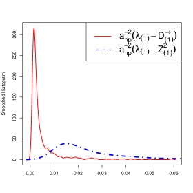
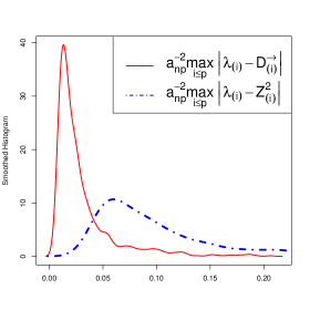
Figure 1. Smoothed histograms of the approximation errors for the normalized eigenvalues $(a_{np}^{-2}\lambda_{(i)})$ for entries $Z_{it}$ with density (3.6), $\alpha=1.6$, $\beta=1$, $n=1,000$ and $p=200$.

The proof of Theorem 3.1 will be given in Section 4. A main step in the proof is provided by the following result whose proof will also be given in Section 4; a version of this theorem was proved in Davis et al. [13] under more restrictive conditions on the growth rate of $(p_{n})$.

Theorem 3.5.

Assume the conditions of Theorem 3.1 on ${\mathbf{Z}}$ and $(p_{n})$.

1. If $\beta\in[0,1]$ we have

   $$a_{np}^{-2}\|{\mathbf{Z}}{\mathbf{Z}}^{\prime}-\operatorname{diag}({\mathbf{Z}}{\mathbf{Z}}^{\prime})\|_{2}\stackrel{{\scriptstyle\mathbb{P}}}{{\rightarrow}}0\,,\qquad n\to\infty\,.$$

2. If $\beta\geq 1$ we have

   $$a_{np}^{-2}\|{\mathbf{Z}}^{\prime}{\mathbf{Z}}-\operatorname{diag}({\mathbf{Z}}^{\prime}{\mathbf{Z}})\|_{2}\stackrel{{\scriptstyle\mathbb{P}}}{{\rightarrow}}0\,,\qquad n\to\infty\,.$$

The second part of this theorem follows from the first one by an interchange of $n$ and $p$. Indeed, if $\beta\geq 1$, we can write $n=p^{1/\beta}\ell(p)$ for some slowly varying function $\ell$ and then part (2) follows from part (1).

Remark 3.6.

Theorem 3.5 shows that the largest eigenvalues of ${\mathbf{Z}}{\mathbf{Z}}^{\prime}$ are determined by the largest diagonal entries. In the case of heavy-tailed Wigner matrices, however, the diagonal elements do not play any particular role.

From this theorem one immediately obtains a result about the approximation of the eigenvalues of ${\mathbf{Z}}{\mathbf{Z}}^{\prime}$ and ${\mathbf{Z}}^{\prime}{\mathbf{Z}}$ by those of $\operatorname{diag}({\mathbf{Z}}{\mathbf{Z}}^{\prime})$ and $\operatorname{diag}({\mathbf{Z}}^{\prime}{\mathbf{Z}})$, respectively. Indeed, for any symmetric $p\times p$ matrices ${\mathbf{A}},{\mathbf{B}}$, by Weyl’s inequality (see Bhatia [8]),

$$\max_{i=1,\ldots,p}\big{|}\lambda_{(i)}({\mathbf{A}}+{\mathbf{B}})-\lambda_{(i)}({\mathbf{A}})\big{|}\leq\|{\mathbf{B}}\|_{2}\,.$$ (3.7)

If we now choose ${\mathbf{A}}+{\mathbf{B}}={\mathbf{Z}}{\mathbf{Z}}^{\prime}$ and ${\mathbf{A}}=\operatorname{diag}({\mathbf{Z}}{\mathbf{Z}}^{\prime})$ (or ${\mathbf{A}}+{\mathbf{B}}={\mathbf{Z}}^{\prime}{\mathbf{Z}}$ and ${\mathbf{A}}=\operatorname{diag}({\mathbf{Z}}^{\prime}{\mathbf{Z}})$) we obtain the following result.

Corollary 3.7.

Assume the conditions of Theorem 3.1 on ${\mathbf{Z}}$ and $(p_{n})$.

1. If $\beta\in[0,1]$ we have

   $$a_{np}^{-2}\,\max_{i=1,\ldots,p}\big{|}\lambda_{(i)}-\lambda_{(i)}(\operatorname{diag}({\mathbf{Z}}{\mathbf{Z}}^{\prime}))\big{|}\stackrel{{\scriptstyle\mathbb{P}}}{{\rightarrow}}0\,,\qquad n\to\infty\,.$$

2. If $\beta>1$ we have

   $$a_{np}^{-2}\,\max_{i=1,\ldots,n}\big{|}\lambda_{(i)}-\lambda_{(i)}(\operatorname{diag}({\mathbf{Z}}^{\prime}{\mathbf{Z}}))\big{|}\stackrel{{\scriptstyle\mathbb{P}}}{{\rightarrow}}0\,,\qquad n\to\infty\,.$$

Now (3.1) and (3.2) are immediate consequences of this corollary. Indeed, we have $\lambda_{(i)}(\operatorname{diag}({\mathbf{Z}}{\mathbf{Z}}^{\prime}))=D_{(i)}^{\rightarrow}$ and $\lambda_{(i)}({\mathbf{Z}}^{\prime}{\mathbf{Z}})=D_{(i)}^{\downarrow}$, $i=1,\ldots,p\wedge n$.

3.2. Point process convergence

In this section we want to illustrate how the approximations from Theorem 3.1 can be used to derive asymptotic theory for the largest eigenvalues of ${\mathbf{Z}}{\mathbf{Z}}^{\prime}$ via the weak convergence of suitable point processes. The limiting point process involves the points of the Poisson process

$$N_{\Gamma}=\sum_{i=1}^{\infty}\varepsilon_{\Gamma_{i}^{-2/\alpha}}\,,\qquad n\to\infty\,,$$ (3.8)

where $\varepsilon_{y}$ is the Dirac measure at $y$,

$$\Gamma_{i}=E_{1}+\cdots+E_{i}\,,\qquad i\geq 1\,,$$

and $(E_{i})$ is a sequence of iid standard exponential random variables. In other words, $N_{\Gamma}$ is a Poisson point process on $(0,\infty)$ with mean measure $\mu(x,\infty)=x^{-\alpha/2}$, $x>0$.

Lemma 3.8.

Assume the conditions of Theorem 3.5 hold.

1. If $\beta\geq 0$, then

   $$\sum_{i=1}^{p}\varepsilon_{a_{np}^{-2}(D_{i}^{\rightarrow}-c_{n})}\stackrel{{\scriptstyle d}}{{\rightarrow}}N_{\Gamma}\,,\qquad n\to\infty\,,$$ (3.9)

   where $c_{n}=0$ if $\mathbb{E}[D^{\rightarrow}]=\infty$ and $c_{n}=\mathbb{E}[D^{\rightarrow}]=n\,\mathbb{E}[Z^{2}]$ otherwise.

2. If $\beta\geq 0$, then

   $$\sum_{i=1}^{p}\varepsilon_{a_{np}^{-2}Z_{(i),np}^{2}}\stackrel{{\scriptstyle d}}{{\rightarrow}}N_{\Gamma}\,,\qquad n\to\infty\,,$$ (3.10)

The weak convergence of the point processes holds in the space of point measures with state space $(0,\infty)$ equipped with the vague topology; see Resnick [29].

Remark 3.9.

Similar results were used in the proofs of Davis et al. [12, 13]. We also mention that the centering $c_{n}$ in the finite variance case can be avoided if $n/a_{np}^{2}\to 0$. The latter condition is satisfied if $\beta>\alpha/2-1$.

Proof.

Part (1) follows from Lemma A.3. As regards part (2), we observe that

$$\sum_{i=1}^{p}\sum_{t=1}^{n}\varepsilon_{a_{np}^{-2}Z_{it}^{2}}\stackrel{{\scriptstyle\rm d}}{{\rightarrow}}N_{\Gamma}\,;$$ (3.11)

see e.g. Resnick [30], Proposition 3.21. On the other hand, $a_{np}^{-2}Z_{(p),np}^{2}\stackrel{{\scriptstyle\mathbb{P}}}{{\rightarrow}}0$ which together with (3.11) yields part (2). ∎

Theorem 3.1 and arguments similar to the proofs in Davis et al. [12, 13] enable one to derive the weak convergence of the point processes of the normalized eigenvalues.

Theorem 3.10.

Assume the conditions of Theorem 3.1. If $\min(\beta,\beta^{-1})\in((\alpha/2-1)_{+},1]$ then

$$\sum_{i=1}^{p}\varepsilon_{a_{np}^{-2}\lambda_{i}}\stackrel{{\scriptstyle\rm d}}{{\rightarrow}}N_{\Gamma}\,,$$ (3.12)

in the space of point measures with state space $(0,\infty)$ equipped with the vague topology.

Proof.

The limit relation (3.12) follows from (3.10) in combination with (3.3). Alternatively, one can exploit (3.9) both for $(D_{i}^{\rightarrow})$ and $(D_{t}^{\downarrow})$ (notice that the point process convergence for the latter sequence follows by interchanging the roles of $n$ and $p$), the fact that $(n\vee p)/a_{np}^{2}\to 0$ if $\min(\beta,\beta^{-1})\in((\alpha/2-1)_{+},1]$ (hence centering of the points $(D_{i}^{\rightarrow})$ and $(D_{t}^{\downarrow})$ in (3.9) can be avoided for $\mathbb{E}[Z^{2}]<\infty$) and finally using the approximations (3.1) or (3.2). ∎

The weak convergence of the point processes of the normalized eigenvalues of ${\mathbf{Z}}{\mathbf{Z}}^{\prime}$ in Theorem 3.10 allows one to use the conventional tools in this field; see Resnick [29, 30]. An immediate consequence is

$$a_{np}^{-2}\big{(}\lambda_{(1)},\ldots,\lambda_{(k)}\big{)}\stackrel{{\scriptstyle\rm d}}{{\rightarrow}}\big{(}\Gamma_{1}^{-2/\alpha},\ldots,\Gamma_{k}^{-2/\alpha}\big{)}$$ (3.13)

for any fixed $k\geq 1$. Using the methods of Davis et al. [12] shows for $\alpha\in(2,4)$

$$a_{np}^{-2}\big{(}\lambda_{(1)}-(p\vee n)\mathbb{E}[Z^{2}],\ldots,\lambda_{(k)}-(p\vee n)\mathbb{E}[Z^{2}]\big{)}\stackrel{{\scriptstyle\rm d}}{{\rightarrow}}\big{(}\Gamma_{1}^{-2/\alpha},\ldots,\Gamma_{k}^{-2/\alpha}\big{)}\,.$$ (3.14)

Equations (3.13) and (3.14) yield that for $\alpha\in(0,4)$ and any fixed $k\geq 1$,

$$a_{np}^{-2}\big{(}\lambda_{(1)}-\lambda_{(2)},\ldots,\lambda_{(k)}-\lambda_{(k+1)}\big{)}\stackrel{{\scriptstyle\rm d}}{{\rightarrow}}\big{(}\Gamma_{1}^{-2/\alpha}-\Gamma_{2}^{-2/\alpha},\ldots,\Gamma_{k}^{-2/\alpha}-\Gamma_{k+1}^{-2/\alpha}\big{)}\,.$$ (3.15)

Related results can also be derived for an increasing number of order statistics, e.g. the joint convergence of the largest eigenvalue $a_{np}^{-2}\lambda_{(1)}$ and the trace $a_{np}^{-2}(\lambda_{1}+\cdots+\lambda_{p})$. In particular, one obtains for $\alpha\in(0,2)$ under the conditions of Theorem 3.10 that

$$\dfrac{\lambda_{(1)}}{\lambda_{1}+\cdots+\lambda_{p}}\stackrel{{\scriptstyle\rm d}}{{\rightarrow}}\dfrac{\Gamma_{1}^{-2/\alpha}}{\Gamma_{1}^{-2/\alpha}+\Gamma_{2}^{-2/\alpha}+\cdots}\,.$$

We refer to Davis et al. [13] for details on the proofs and more examples.

In the next subsection we will show how the above results on the joint convergence of eigenvalues can be applied to approximate the eigenvectors of ${\mathbf{Z}}{\mathbf{Z}}^{\prime}$.

3.3. Eigenvectors

In this section we assume the conditions of Theorem 3.5 and $\beta\in[0,1]$. From Theorem 3.5(1) we know that ${\mathbf{Z}}{\mathbf{Z}}^{\prime}$ is approximated in spectral norm by $\operatorname{diag}({\mathbf{Z}}{\mathbf{Z}}^{\prime})$. The unit eigenvectors of a $p\times p$ diagonal matrix are the canonical basis vectors ${\mathbf{e}}_{j}\in\mathbb{R}^{p}$, $j=1,\dots,p$. This raises the question as to whether $({\mathbf{e}}_{j})$ are good approximations of the eigenvectors $({\mathbf{v}}_{j})$ of ${\mathbf{Z}}{\mathbf{Z}}^{\prime}$. By ${\mathbf{v}}_{{j}}$ we denote the unit eigenvector associated with the $j$th largest eigenvalue $\lambda_{(j)}$. The unit eigenvector associated with the $j$th largest eigenvalue of $\operatorname{diag}({\mathbf{Z}}{\mathbf{Z}}^{\prime})$ is ${\mathbf{e}}_{L_{j}}$, where $L_{j}$ is defined in (2.3). Our guess that ${\mathbf{v}}_{j}$ is approximated by ${\mathbf{e}}_{L_{j}}$ is confirmed by the following result.

Theorem 3.11.

Assume the conditions of Theorem 3.1 and let $\beta\in[0,1]$. Then for any fixed $k\geq 1$,

$$\|{\mathbf{v}}_{k}-{\mathbf{e}}_{L_{k}}\|_{\ell_{2}}\stackrel{{\scriptstyle\mathbb{P}}}{{\rightarrow}}0\,,\quad n\to\infty\,.$$

Indeed, ${\mathbf{v}}_{j}$ and ${\mathbf{e}}_{L_{j}}$ share another property: they are localized which means that they are concentrated only in a few components. Vectors which are not localized are called delocalized. Figure 2 shows the outcome of a simulation example in which we visualize the components of the unit eigenvector associated with the largest eigenvalue of ${\mathbf{Z}}{\mathbf{Z}}^{\prime}$ for a simulated data matrix ${\mathbf{Z}}$ with iid Pareto(0.8) entries. In the right graph we see that only one of the $p=200$ components is significant. Hence we can find a canonical basis vector ${\mathbf{e}}_{k}$ such that $\|{\mathbf{e}}_{k}-{\mathbf{v}}_{1}\|_{\ell_{2}}$ is small. Therefore the eigenvector is localized. This is in stark contrast to the case of iid standard normal entries; see the left graph. Then many components are of similar magnitude, hence the eigenvector is delocalized. Typically, the eigenvectors tend to be localized when the entry distribution has an infinite fourth moment, while they tend to be delocalized otherwise; see Benaych-Georges and Péché [7] for the case of Wigner matrices.

Figure 2. The components of the eigenvector ${\mathbf{v}}_{1}$. Right: The case of iid Pareto(0.8) entries. Left: The case of iid standard normal entries. We choose $p=200$ and $n=1,000$.

Proof of Theorem 3.11.

Fix $k\geq 1$. Since $p\to\infty$ we can assume $k\leq p$ for sufficiently large $n$. We observe that

$${\mathbf{Z}}{\mathbf{Z}}^{\prime}\,{\mathbf{e}}_{j}-D^{\rightarrow}_{j}\,{\mathbf{e}}_{j}=\Big{(}\sum_{t=1}^{n}Z_{1t}Z_{jt},\ldots,\sum_{t=1}^{n}Z_{j-1,t}Z_{jt},0,\sum_{t=1}^{n}Z_{j+1,t}Z_{jt},\ldots,\sum_{t=1}^{n}Z_{pt}Z_{jt}\Big{)}^{\prime}\,,\quad j=1,\ldots,p\,,$$

are the columns of ${\mathbf{Z}}{\mathbf{Z}}^{\prime}-\operatorname{diag}({\mathbf{Z}}{\mathbf{Z}}^{\prime})$. By Theorem 3.5(1),

$$a_{np}^{-2}\max_{j=1,\ldots,p}\|{\mathbf{Z}}{\mathbf{Z}}^{\prime}{\mathbf{e}}_{j}-D^{\rightarrow}_{j}{\mathbf{e}}_{j}\|_{\ell_{2}}\leq a_{np}^{-2}\|{\mathbf{Z}}{\mathbf{Z}}^{\prime}-\operatorname{diag}({\mathbf{Z}}{\mathbf{Z}}^{\prime})\|_{2}\stackrel{{\scriptstyle\mathbb{P}}}{{\rightarrow}}0\,,\qquad n\to\infty\,.$$ (3.16)

If we set ${\mathbf{H}}^{(n)}=a_{np}^{-2}{\mathbf{Z}}{\mathbf{Z}}^{\prime}$, ${\mathbf{v}}^{(n)}={\mathbf{e}}_{L_{k}}\in\mathbb{R}^{p}$ and $\lambda^{(n)}=a_{np}^{-2}D^{\rightarrow}_{L_{k}}$, we see that

$$a_{np}^{-2}{\mathbf{Z}}{\mathbf{Z}}^{\prime}{\mathbf{e}}_{L_{k}}=a_{np}^{-2}D^{\rightarrow}_{L_{k}}{\mathbf{e}}_{L_{k}}+\varepsilon^{(n)}{\mathbf{w}}^{(n)},$$

where ${\mathbf{w}}^{(n)}=\|{\mathbf{Z}}{\mathbf{Z}}^{\prime}{\mathbf{e}}_{L_{k}}-D^{\rightarrow}_{L_{k}}{\mathbf{e}}_{L_{k}}\|_{\ell_{2}}^{-1}({\mathbf{Z}}{\mathbf{Z}}^{\prime}{\mathbf{e}}_{L_{k}}-D^{\rightarrow}_{L_{k}}{\mathbf{e}}_{L_{k}})$ is a unit vector and $\varepsilon^{(n)}=a_{np}^{-2}\|{\mathbf{Z}}{\mathbf{Z}}^{\prime}{\mathbf{e}}_{L_{k}}-D^{\rightarrow}_{L_{k}}{\mathbf{e}}_{L_{k}}\|_{\ell_{2}}\stackrel{{\scriptstyle\mathbb{P}}}{{\rightarrow}}0$ by (3.16).

Before we can apply Proposition A.7 we need to show that with probability converging to $1$, there are no other eigenvalues in a suitably small interval around $\lambda_{(k)}$. Let $s>1$. We define the set

$$\Omega_{n}=\Omega_{n}(k,s)=\{a_{np}^{-2}|\lambda_{(k)}-\lambda_{(i)}|>s\,\varepsilon^{(n)}\,:\,i\neq k=1,\ldots,p\}\,.$$

From (3.16) we get $s\,\varepsilon^{(n)}\to 0$. Then using this and (3.15), we obtain

$$\begin{split}\lim_{n\to\infty}\mathbb{P}(\Omega_{n}^{c})&=\lim_{n\to\infty}\mathbb{P}(a_{np}^{-2}\min\{\lambda_{(k-1)}-\lambda_{(k)},\lambda_{(k)}-\lambda_{(k+1)}\}\leq s\,\varepsilon^{(n)})=0\end{split}$$

By Proposition A.7 the unit eigenvector ${\mathbf{v}}_{k}$ associated with $\lambda_{(k)}$ and the projected vector ${\mathbf{P}}_{{\mathbf{e}}_{L_{k}}}({\mathbf{v}}_{k})=({\mathbf{v}}_{k})_{L_{k}}{\mathbf{e}}_{L_{k}}$ satisfy for fixed $\delta>0$:

$$\begin{split}\limsup_{n\to\infty}\mathbb{P}(\|{\mathbf{v}}_{k}-({\mathbf{v}}_{k})_{L_{k}}{\mathbf{e}}_{L_{k}}\|_{\ell_{2}}>\delta)&\leq\limsup_{n\to\infty}\mathbb{P}(\{\|{\mathbf{v}}_{k}-({\mathbf{v}}_{k})_{L_{k}}{\mathbf{e}}_{L_{k}}\|_{\ell_{2}}>\delta\}\cap\Omega_{n})+\limsup_{n\to\infty}\mathbb{P}(\Omega_{n}^{c})\\ &\leq\limsup_{n\to\infty}\mathbb{P}(\{2\varepsilon^{(n)}/(s\,\varepsilon^{(n)}-\varepsilon^{(n)})>\delta\}\cap\Omega_{n})\\ &\leq\limsup_{n\to\infty}\mathbb{P}(\{2/(s-1)>\delta\})=\mathbf{1}_{\{2/(s-1)>\delta\}}.\end{split}$$

The right-hand side is zero for sufficiently large $s$. Since both ${\mathbf{v}}_{k}$ and ${\mathbf{e}}_{L_{k}}$ are unit vectors this means that

$$\|{\mathbf{v}}_{k}-{\mathbf{e}}_{L_{k}}\|_{\ell_{2}}\stackrel{{\scriptstyle\mathbb{P}}}{{\rightarrow}}0\,,\quad n\to\infty\,.$$

This proves our result on eigenvectors. ∎

4. Proof of Theorem 3.1

In what follows, $c$ stands for any constant whose value is not of interest. We write $(Z_{t})$ for an iid sequence with the same distribution as $Z$.

The plan of the proof is as follows:

1. We prove Theorem 3.5 which implies (3.1) and (3.2); see Corollary 3.7. In view of the arguments after Theorem 3.1 it suffices to consider only the case $\beta\in[0,1]$.

2. We prove (3.3).

4.1. Proof of Theorem 3.5

We proceed in several steps.

The case $\alpha\in(0,8/3)$.

If $\alpha\in[1,2)$ and $\mathbb{E}[|Z|]<\infty$, we have

$$a_{np}^{-1}\|{\mathbf{Z}}-({\mathbf{Z}}-\mathbb{E}[{\mathbf{Z}}])\|_{2}=|\mathbb{E}[Z]|\frac{\sqrt{np}}{a_{np}}\to 0\,,\quad n\to\infty.$$

Therefore, without loss of generality $\mathbb{E}[Z]$ can be assumed $0$ in this case.

From now on we assume $\mathbb{E}[Z]=0$ whenever $\mathbb{E}[|Z|]$ exists. Since the Frobenius norm $\|\cdot\|_{F}$ is an upper bound of the spectral norm we have

$$\|{\mathbf{Z}}{\mathbf{Z}}^{\prime}-\operatorname{diag}({\mathbf{Z}}{\mathbf{Z}}^{\prime})\|_{2}^{2} \leq \|{\mathbf{Z}}{\mathbf{Z}}^{\prime}-\operatorname{diag}({\mathbf{Z}}{\mathbf{Z}}^{\prime})\|_{F}^{2}$$

$$= \sum_{i,j=1;i\neq j}^{p}\sum_{t=1}^{n}Z_{it}^{2}Z_{jt}^{2}+\sum_{i,j=1;i\neq j}^{p}\sum_{t_{1},t_{2}=1;t_{1}\neq t_{2}}^{n}Z_{i,t_{1}}Z_{j,t_{1}}Z_{i,t_{2}}Z_{j,t_{2}}$$

$$= \sum_{i,j=1;i\neq j}^{p}\sum_{t=1}^{n}Z_{it}^{2}Z_{jt}^{2}\big{[}\mathbf{1}_{\{Z_{it}^{2}Z_{jt}^{2}>a_{np}^{4}\}}+\mathbf{1}_{\{Z_{it}^{2}Z_{jt}^{2}\leq a_{np}^{4}\}}\big{]}+I_{2}^{(n)}$$

$$= I_{11}^{(n)}+I_{12}^{(n)}+I_{2}^{(n)}\,.$$

Thus it suffices to show that each of the expressions on the right-hand side when normalized with $a_{np}^{4}$ converges to zero in probability. We have for any $\epsilon>0$,

$$\mathbb{P}\big{(}I_{11}^{(n)}>\epsilon\,a_{np}^{4}\big{)}\leq p^{2}\,n\,\mathbb{P}(Z_{1}^{2}Z_{2}^{2}>a_{np}^{4})\to 0\,.$$

Here we also used the fact that $Z_{1}Z_{2}$ is regularly varying with index $\alpha$; see Embrechts and Goldie [17]. An application of Markov’s inequality and Lyapunov’s moment inequality with $\gamma\in(\alpha/2,4/3)$ if $\alpha\in[2,8/3)$ and $\gamma=1$ otherwise shows that

$$\mathbb{P}\big{(}I_{12}^{(n)}>\epsilon\,a_{np}^{4}\big{)}\leq c\,\frac{p^{2}n}{a_{np}^{4}}\Big{(}\mathbb{E}[|Z_{1}Z_{2}|^{2\gamma}\mathbf{1}_{\{|Z_{1}Z_{2}|\leq a_{np}^{2}\}}]\Big{)}^{\frac{1}{\gamma}}\leq c\,p^{2-\frac{2}{\gamma}}\,n^{1-\frac{2}{\gamma}+\delta}\to 0,$$

where we used Karamata’s theorem (see Bingham et al. [9]), and the constant $\delta>0$ can be chosen arbitrarily small due to the Potter bounds.

In the case $\alpha\in(0,2)$ the probability $P_{2}^{(n)}=\mathbb{P}(I_{2}^{(n)}>\epsilon\,a_{np}^{4})$ can be handled analogously. Next, we turn to $P_{2}^{(n)}$ in the case $\alpha\in(2,8/3)$. In particular, $\mathbb{E}[Z^{2}]<\infty$. With Čebychev’s inequality, also using the fact that $\mathbb{E}[Z]=0$, we find that

$$P_{2}^{(n)}\leq c\frac{1}{a_{np}^{8}}\mathbb{E}\Big{[}\Big{(}\sum_{i,j=1;i\neq j}^{p}\sum_{t_{1},t_{2}=1;t_{1}\neq t_{2}}^{n}Z_{i,t_{1}}Z_{j,t_{1}}Z_{i,t_{2}}Z_{j,t_{2}}\Big{)}^{2}\Big{]}\leq c\,\frac{(p\,n)^{2}}{a_{np}^{8}}\to 0.$$ (4.17)

The case $\alpha=2$ is most difficult because the second moment of $Z$ can be infinite. Without loss of generality we assume that $Z$ is continuous. Otherwise, we add independent centered normal random variables to each of the entries $Z_{it}$; due the normalization $a_{np}^{2}$ the asymptotic properties of the eigenvalues remain the same, i.e., the added normal components are asymptotically negligible. In view of Hult and Samorodnitsky [20, Lemma $4.2$] there exist constants $C,K>0$ and a function $h:[K,\infty)\to(0,\infty)$ such that

$$\mathbb{E}[Z\mathbf{1}_{\{-h(x)\leq Z\leq x\}}]=0\quad\mbox{and}\quad C^{-1}\leq\frac{h(x)}{x}\leq C$$ (4.18)

for all $x\geq K$. We have

$$I_{2}^{(n)} = \sum_{i,j=1;i\neq j}^{p}\sum_{t_{1},t_{2}=1;t_{1}\neq t_{2}}^{n}Z_{i,t_{1}}Z_{j,t_{1}}Z_{i,t_{2}}Z_{j,t_{2}}\,\big{[}\mathbf{1}_{A_{i,j,t_{1},t_{2}}^{c}}+\mathbf{1}_{A_{i,j,t_{1},t_{2}}}\big{]}=I_{21}^{(n)}+I_{22}^{(n)}\,,$$

where $A_{i,j,t_{1},t_{2}}=\{-h(a_{np}^{4})\leq Z_{i,t_{1}},Z_{j,t_{1}},Z_{i,t_{2}},Z_{j,t_{2}}\leq a_{np}^{4}\}$. We see that

$$\mathbb{P}(I_{21}^{(n)}>\epsilon\,a_{np}^{4}) \leq (p\,n)^{2}\,\mathbb{P}(A_{i,j,t_{1},t_{2}}^{c})\leq c\,(p\,n)^{2}\,\mathbb{P}(|Z|>\min(h(a_{np}^{4}),a_{np}^{4}))$$

$$\leq c\,(pn)^{2}\,\mathbb{P}(|Z|>\min(C,C^{-1})\,a_{np}^{4})\leq c\,(np)^{-2+\delta}\to 0,$$

where we used the second formula in (4.18). The small constant $\delta>0$ comes from a Potter bound argument. Finally, using the first condition in (4.18), we may conclude similarly to (4.17) that

$$P_{22}^{(n)}=\mathbb{P}(I_{22}^{(n)}>\epsilon\,a_{np}^{4})\leq c\,\frac{(pn)^{2}}{a_{np}^{8}}\,\big{(}\mathbb{E}[Z^{2}\mathbf{1}_{\{-h(a_{np}^{4})\leq Z\leq a_{np}^{4}\}}]\big{)}^{4}.$$

Since

$$\mathbb{E}[Z^{2}\mathbf{1}_{\{|Z|\leq\max(C,C^{-1})x\}}]\geq\mathbb{E}[Z^{2}\mathbf{1}_{\{-h(x)\leq Z\leq x\}}]\,,$$

and the left-hand side is slowly varying (see [18]), we have $P_{22}^{(n)}\to 0$. The proof is complete for $\alpha\in(0,8/3)$. ∎

The case $\alpha\in[8/3,4)$

Before we can proceed with the case $\alpha\in[8/3,4)$ we provide an auxiliary result. Consider the following decomposition

$$[{\mathbf{Z}}{\mathbf{Z}}^{\prime}-\operatorname{diag}({\mathbf{Z}}{\mathbf{Z}}^{\prime})]^{2}={\mathbf{D}}+{\mathbf{F}}+{\mathbf{R}}\,,$$

where

$${\mathbf{D}}=(D_{ij})_{i,j=1,\ldots,p}=\operatorname{diag}([{\mathbf{Z}}{\mathbf{Z}}^{\prime}-\operatorname{diag}({\mathbf{Z}}{\mathbf{Z}}^{\prime})]^{2})\,,$$

The $p\times p$ matrix ${\mathbf{F}}$ has a zero-diagonal and

$$F_{ij}=\sum_{u=1;u\neq i,j}^{p}\sum_{t=1}^{n}Z_{it}\,Z_{jt}\,Z_{ut}^{2},\quad 1\leq i\neq j\leq p\,,$$

The $p\times p$ matrix ${\mathbf{R}}$ has a zero-diagonal and

$$R_{ij}=\sum_{u=1;u\neq i,j}^{p}\sum_{t_{1}=1}^{n}\sum_{t_{2}=1;t_{2}\neq t_{1}}^{n}Z_{i,t_{1}}\,Z_{j,t_{2}}\,Z_{u,t_{1}}\,Z_{u,t_{2}},\quad 1\leq i\neq j\leq p\,.$$

Lemma 4.1.

Assume the conditions of Theorem 3.5 and $\alpha\in(2,4)$. Then $a_{np}^{-4}\big{(}\|{\mathbf{D}}\|_{2}+\|{\mathbf{F}}\|_{2}+\|{\mathbf{R}}\|_{2}\big{)}\stackrel{{\scriptstyle\mathbb{P}}}{{\rightarrow}}0$.

In view of this lemma we have

$$a_{np}^{-4}\|{\mathbf{Z}}{\mathbf{Z}}^{\prime}-\operatorname{diag}({\mathbf{Z}}{\mathbf{Z}}^{\prime})\|_{2}^{2}=a_{np}^{-4}\|[{\mathbf{Z}}{\mathbf{Z}}^{\prime}-\operatorname{diag}({\mathbf{Z}}{\mathbf{Z}}^{\prime})]^{2}\|_{2}=a_{np}^{-4}\|{\mathbf{D}}+{\mathbf{F}}+{\mathbf{R}}\|_{2}^{2}\stackrel{{\scriptstyle\mathbb{P}}}{{\rightarrow}}0\,.$$

This finishes the proof of Theorem 3.5. It is left to prove Lemma 4.1.

Proof of the ${\mathbf{D}}$-part.

We have for $i=1,\ldots,p$,

$$\begin{split}D_{ii}&=\sum_{u=1}^{p}\sum_{t=1}^{n}Z_{it}^{2}Z_{ut}^{2}\mathbf{1}_{\{i\neq u\}}+\sum_{u=1}^{p}\sum_{t_{1}=1}^{n}\sum_{t_{2}=1}^{n}Z_{i,t_{1}}Z_{u,t_{1}}Z_{u,t_{2}}Z_{i,t_{2}}\mathbf{1}_{\{i\neq u\}}\mathbf{1}_{\{t_{1}\neq t_{2}\}}=M_{ii}+N_{ii}\,.\end{split}$$

We write ${\mathbf{M}}$ and ${\mathbf{N}}$ for diagonal matrices constructed from $(M_{ii})$ and $(N_{ii})$ such that ${\mathbf{D}}={\mathbf{M}}+{\mathbf{N}}$. First bounding $\|{\mathbf{N}}\|_{2}$ by the Frobenius norm and then applying Markov’s inequality, one can prove that $a_{np}^{-4}\|{\mathbf{N}}\|_{2}\stackrel{{\scriptstyle\mathbb{P}}}{{\rightarrow}}0$. We have

$$\frac{\mathbb{E}[M_{ii}]}{a_{np}^{4}}\leq c\,\frac{np}{a_{np}^{4}}\to 0,\qquad n\to\infty.$$

Therefore centering of $M_{ii}$ will not influence the limit of the spectral norm $a_{np}^{-4}\|{\mathbf{M}}\|_{2}$. Writing $A_{i,u}=\{|\sum_{t=1}^{n}(Z_{it}^{2}Z_{ut}^{2}-\mathbb{E}[Z_{1}^{2}Z_{2}^{2}])\mathbf{1}_{\{i\neq u\}}|>a_{np}^{2}\}$, we have for $i=1,\ldots,p$,

$$M_{ii}-\mathbb{E}[M_{ii}] = \sum_{u=1}^{p}\sum_{t=1}^{n}\big{(}Z_{it}^{2}Z_{ut}^{2}-\mathbb{E}[Z_{1}^{2}Z_{2}^{2}]\big{)}\,\mathbf{1}_{\{i\neq u\}}\,\big{[}\mathbf{1}_{A_{i,u}}+\mathbf{1}_{A_{i,u}^{c}}\big{]}$$

$$= M_{ii}^{(1)}+M_{ii}^{(2)}.$$

On the one hand, $\|M^{(2)}\|_{2}\leq p\,a_{np}^{2}$. Hence $a_{np}^{-4}\|M^{(2)}\|_{2}\stackrel{{\scriptstyle\mathbb{P}}}{{\rightarrow}}0$. On the other hand, we obtain with Markov’s inequality, Proposition A.2 and the Potter bounds for $\epsilon>0$ and small $\delta>0$,

$$\mathbb{P}(\|M^{(1)}\|_{2}>\epsilon\,a_{np}^{4}) = \mathbb{P}(\max_{i=1,\ldots,p}|M_{ii}^{(1)}|>\epsilon\,a_{np}^{4})$$

$$\leq \mathbb{P}\Big{(}\max_{i=1,\ldots,p}\sum_{u=1}^{p}\Big{|}\sum_{t=1}^{n}(Z_{it}^{2}Z_{ut}^{2}-\mathbb{E}[Z_{1}^{2}Z_{2}^{2}])\mathbf{1}_{\{i\neq u\}}\,\mathbf{1}_{A_{i,u}}\Big{|}>\epsilon\,a_{np}^{4}\Big{)}$$

$$\leq c\frac{p^{2}}{a_{np}^{4}}\mathbb{E}\Big{[}\Big{|}\sum_{t=1}^{n}(Z_{1t}^{2}Z_{2t}^{2}-\mathbb{E}[Z_{1}^{2}Z_{2}^{2}])\Big{|}\mathbf{1}_{A_{1,2}}\Big{]}$$

$$\sim c\,\frac{p^{2}}{a_{np}^{4}}\,n\,a_{np}^{2}\,\mathbb{P}(Z_{1}^{2}Z_{2}^{2}>a_{np}^{2})\leq\dfrac{p\,(np)^{\delta}}{a_{np}^{2}}\to 0,$$

since $Z_{1}Z_{2}$ is regularly varying with index $\alpha$. This finishes the proof of the ${\mathbf{D}}$-part. ∎

Proof of the ${\mathbf{F}}$-part.

Let $\delta>0$. We will use the following decomposition for $i\neq j$:

$$F_{ij}=\sum_{u=1;u\neq i,j}^{p}\sum_{t=1}^{n}Z_{it}Z_{jt}(Z_{ut}^{2}-\mathbb{E}[Z^{2}\mathbf{1}_{\{Z^{2}\leq a_{np}^{4-2\delta}\}}])+\mathbb{E}[Z^{2}\mathbf{1}_{\{Z^{2}\leq a_{np}^{4-2\delta}\}}]\,(p-2)\sum_{t=1}^{n}Z_{it}Z_{jt}=\widetilde{F}_{ij}+T_{ij}\,.$$

We observe that ${\mathbf{T}}=\mathbb{E}[Z^{2}\mathbf{1}_{\{Z^{2}\leq a_{np}^{4-2\delta}\}}]\,(p-2)\,({\mathbf{Z}}_{n}{\mathbf{Z}}_{n}^{\prime}-\operatorname{diag}({\mathbf{Z}}_{n}{\mathbf{Z}}_{n}^{\prime}))$. We have for some constant $c>0$,

$$\|{\mathbf{T}}\|_{2}^{2} = \|{\mathbf{T}}^{2}\|_{2}\leq c\,p^{2}\,\|({\mathbf{Z}}_{n}{\mathbf{Z}}_{n}^{\prime}-\operatorname{diag}({\mathbf{Z}}_{n}{\mathbf{Z}}_{n}^{\prime}))^{2}\|_{2}$$

$$\leq c\,p^{2}\,\|{\mathbf{D}}+\widetilde{\mathbf{F}}+{\mathbf{R}}\|_{2}+c\,p^{2}\,\|{\mathbf{T}}\|_{2}\,.$$

Therefore

$$\dfrac{\|{\mathbf{T}}\|_{2}}{a_{np}^{4}}\leq c\,\dfrac{p}{a_{np}^{2}}\,\Big{(}\dfrac{\|{\mathbf{D}}+\widetilde{\mathbf{F}}+{\mathbf{R}}\|_{2}}{a_{np}^{4}}\Big{)}^{1/2}+c\,\dfrac{p}{a_{np}^{2}}\Big{(}\dfrac{\|{\mathbf{T}}\|_{2}}{a_{np}^{4}}\Big{)}^{1/2}\,.$$ (4.19)

In the course of the proof of this lemma we show that

$$\dfrac{\|{\mathbf{D}}+\widetilde{\mathbf{F}}+{\mathbf{R}}\|_{2}}{a_{np}^{4}}\stackrel{{\scriptstyle\mathbb{P}}}{{\rightarrow}}0\,.$$

Moreover, there is a small $\varepsilon>0$ such that

$$\delta_{n}=\frac{p}{a_{np}^{2}}\leq n^{1-4/\alpha+\varepsilon},\quad 1-4/\alpha+\varepsilon<0\,.$$

Therefore iteration of (4.19) yields for $k\geq 1$

$$\dfrac{\|{\mathbf{T}}\|_{2}}{a_{np}^{4}} \leq o_{\mathbb{P}}(1)+c\,\delta_{n}\Big{(}\delta_{n}\,\Big{(}\dfrac{\|{\mathbf{D}}+\widetilde{\mathbf{F}}+{\mathbf{R}}\|_{2}}{a_{np}^{4}}\Big{)}^{1/2}\Big{)}^{1/2}+c\,\delta_{n}\Big{(}\delta_{n}\Big{(}\dfrac{\|{\mathbf{T}}\|_{2}}{a_{np}^{4}}\Big{)}^{1/2}\Big{)}^{1/2}$$ (4.20)

$$= o_{\mathbb{P}}(1)+c\,\Big{(}\delta_{n}^{4+2}\dfrac{\|{\mathbf{T}}\|_{2}}{a_{np}^{4}}\Big{)}^{1/4}$$

$$\leq o_{\mathbb{P}}(1)+c\,\Big{(}\delta_{n}^{2^{k}+\cdots+2}\dfrac{\|{\mathbf{T}}\|_{2}}{a_{np}^{4}}\Big{)}^{1/{2^{k}}}\,.$$

Using some elementary moment bounds for $\|{\mathbf{T}}\|_{2}$ (e.g. a bound by the Frobenius norm), it is not difficult to show that $n^{-l}\|{\mathbf{T}}\|_{2}\stackrel{{\scriptstyle\mathbb{P}}}{{\rightarrow}}0$ for some sufficiently large $l$. Thus we achieve that the right-hand side in (4.20) converges to zero in probability.

It remains to show that $a_{np}^{-4}\|\widetilde{{\mathbf{F}}}\|_{2}\stackrel{{\scriptstyle\mathbb{P}}}{{\rightarrow}}0$. With the notation $B_{u,t}=\{Z_{ut}^{2}\leq a_{np}^{4-2\delta}\}$ for some small $\delta>0$, we decompose $Z_{it}Z_{jt}(Z_{ut}^{2}-\mathbb{E}[Z^{2}\mathbf{1}_{\{Z^{2}\leq a_{np}^{4-2\delta}\}}])$ as follows:

$$\begin{split}&Z_{it}Z_{jt}(Z_{ut}^{2}\mathbf{1}_{B_{u,t}}-\mathbb{E}[Z^{2}\mathbf{1}_{\{Z^{2}\leq a_{np}^{4-2\delta}\}}])+Z_{it}Z_{jt}Z_{ut}^{2}\mathbf{1}_{B_{u,t}^{c}}\,.\end{split}$$

We decompose the matrix $\widetilde{{\mathbf{F}}}$ accordingly:

$$\widetilde{{\mathbf{F}}}=\widetilde{{\mathbf{F}}}^{(1)}+\widetilde{{\mathbf{F}}}^{(2)}\,,$$

such that, for example,

$$\widetilde{F}^{(1)}_{ij}=\sum_{u=1;u\neq i,j}^{p}\sum_{t=1}^{n}Z_{it}Z_{jt}(Z_{ut}^{2}\mathbf{1}_{B_{u,t}}-\mathbb{E}[Z^{2}\mathbf{1}_{\{Z^{2}\leq a_{np}^{4-2\delta}\}}])\,,\quad i\neq j.$$

$\widetilde{{\mathbf{F}}}^{(1)}$: Bounding the spectral norm by the Frobenius norm, applying Markov’s inequality and using Karamata’s theorem together with the Potter bounds one can check that for $\epsilon>0$ and small $\delta>0$,

$$\begin{split}\mathbb{P}&(\|\widetilde{{\mathbf{F}}}^{(1)}\|_{2}>\epsilon\,a_{np}^{4})\leq c\,a_{np}^{-8}\,\mathbb{E}\Big{[}\sum_{i,j=1}^{p}(\widetilde{F}^{(1)}_{ij})^{2}\Big{]}\\ &\leq c\,\frac{p^{3}\,n}{a_{np}^{8}}\mathbb{E}[(Z_{1}Z_{2})^{2}]\mathbb{E}[(Z^{2}\mathbf{1}_{\{Z^{2}\leq a_{np}^{4-2\delta}\}}-\mathbb{E}[Z^{2}\mathbf{1}_{\{Z^{2}\leq a_{np}^{4-2\delta}\}}])^{2}]\\ &\leq c\,\frac{p^{3}\,n}{a_{np}^{8}}\mathbb{E}[Z^{4}\mathbf{1}_{\{Z^{2}\leq a_{np}^{4-2\delta}\}}]\\ &\leq c\frac{p^{3}n}{a_{np}^{4\delta}}\mathbb{P}(|Z|>a_{np}^{2-\delta})\to 0\,,\qquad n\to\infty,\end{split}$$

$\widetilde{{\mathbf{F}}}^{(2)}$: We have for small $\delta>0$,

$$\mathbb{P}(\|\widetilde{{\mathbf{F}}}^{(2)}\|_{2}>\epsilon\,a_{np}^{4}) \leq \mathbb{P}\Big{(}\bigcup_{1\leq u\leq p\,,1\leq t\leq n}B_{u,t}^{c}\Big{)}$$

$$\leq p\,n\,\mathbb{P}(|Z|>a_{np}^{2-\delta})\to 0\,,\qquad\,n\to\infty\,.$$

The proof of the ${\mathbf{F}}$-part is complete. ∎

Proof of the ${\mathbf{R}}$-part.

We have

$$\mathbb{E}[\|{\mathbf{R}}\|_{2}^{2}]\leq\mathbb{E}[\|{\mathbf{R}}\|_{F}^{2}] \leq \sum_{i,j=1}^{p}\sum_{u=1}^{p}\sum_{t_{1}=1}^{n}\sum_{t_{2}=1}^{n}(\mathbb{E}[Z^{2}])^{4}\leq c\,p^{3}\,n^{2}\,.$$

Therefore and by Markov’s inequality for $\epsilon>0$,

$$\mathbb{P}(\|{\mathbf{R}}\|_{2}>\epsilon\,a_{np}^{4})\leq c\,\frac{p^{3}\,n^{2}}{a_{np}^{8}}\to 0,\qquad n\to\infty\,,$$ (4.21)

as long as $\alpha\in(2,16/5)$. For $\alpha\in[16/5,4)$ we use a similar idea for the truncated entries. Write ${\mathbf{R}}=\overline{{\mathbf{R}}}+\widetilde{{\mathbf{R}}}$, where for $i\neq j$

$$\begin{split}\overline{R}_{ij}&=\sum_{u=1;u\neq i,j}^{p}\sum_{t_{1}=1}^{n}\sum_{t_{1}=1;t_{1}\neq t_{2}}^{n}Z_{i,t_{1}}Z_{j,t_{2}}Z_{u,t_{1}}Z_{u,t_{2}}\,\mathbf{1}_{A_{i,j,t_{1},t_{2}}},\\ \widetilde{R}_{ij}&=\sum_{u=1;u\neq i,j}^{p}\sum_{t_{1}=1}^{n}\sum_{t_{1}=1;t_{1}\neq t_{2}}^{n}Z_{i,t_{1}}Z_{j,t_{2}}Z_{u,t_{1}}Z_{u,t_{2}}\,\mathbf{1}_{A_{i,j,t_{1},t_{2}}^{c}},\end{split}$$

with $A_{i,j,t_{1},t_{2}}^{c}=\{-h(a_{np})\leq Z_{i,t_{1}},Z_{j,t_{2}},Z_{u,t_{1}},Z_{u,t_{2}}\leq a_{np}\}$ and $h$ as in (4.18). Analogously to (4.21), using the fact that the random variables $Z_{i,t_{1}}Z_{j,t_{2}}Z_{u,t_{1}}Z_{u,t_{2}}\,\mathbf{1}_{A_{i,j,t_{1},t_{2}}}$ are uncorrelated for the considered index set, one obtains for $\epsilon>0$,

$$\mathbb{P}(\|\overline{{\mathbf{R}}}\|_{2}>\epsilon\,a_{np}^{4}) \leq c\,\frac{p^{3}\,n^{2}}{a_{np}^{8}}\,\mathbb{E}[Z^{2}\mathbf{1}_{\{|Z|>\min(C,C^{-1})\,a_{np}\}}]$$

$$\leq c\,\frac{p^{3}\,n^{2}}{a_{np}^{6}}\,\mathbb{P}(|Z|>\min(C,C^{-1})\,a_{np})\to 0$$

as $n\to\infty$, where we used Karamata’s theorem and $\mathbb{P}(A_{i,j,t_{1},t_{2}})\leq c\,\mathbb{P}(|Z|>\min(C,C^{-1})\,a_{np})$.

We introduce the truncated random variables $\widetilde{Z}_{it}=Z_{it}\mathbf{1}_{\{-h(a_{np})\leq Z_{it}\leq a_{np}\}}$ with generic element $\widetilde{Z}$. We will repeatedly use the following inequality which is valid for a real symmetric matrix ${\mathbf{M}}$:

$$\|{\mathbf{M}}\|_{2}^{2}\leq\|{\mathbf{M}}\|_{F}^{2}=\operatorname{tr}({\mathbf{M}}^{2}).$$

Then we have for $k\geq 1$, $\|\widetilde{{\mathbf{R}}}^{2^{k-1}}\|_{2}^{2}=\|\widetilde{{\mathbf{R}}}^{2^{k}}\|_{2}$ and

$$\|\widetilde{{\mathbf{R}}}\|_{2}^{2^{k}}\leq\operatorname{tr}(\widetilde{{\mathbf{R}}}^{2^{k}})=\sum_{i,j=1}^{p}(\widetilde{R}^{2^{k-1}})_{ij}^{2}\,.$$

This together with the Markov inequality of order $2^{k}$ yields

$$\mathbb{P}(\|\widetilde{{\mathbf{R}}}\|_{2}>ca_{np}^{4})\leq ca_{np}^{-4\cdot 2^{k}}\mathbb{E}\Big{[}\sum_{i,j=1}^{p}(\widetilde{R}^{2^{k-1}})_{ij}^{2}\Big{]}.$$ (4.22)

Next we study the structure of $\widetilde{{\mathbf{R}}}^{2^{k-1}}$. The $(i,j)$-entry of this matrix is

$$(\widetilde{R}^{2^{k-1}})_{ij}=\sum_{i_{1}=1}^{p}\cdots\sum_{i_{2^{k-1}-1}=1}^{p}\widetilde{R}_{i,i_{1}}\widetilde{R}_{i_{1},i_{2}}\cdots\widetilde{R}_{i_{2^{k-1}-2},i_{2^{k-1}-1}}\widetilde{R}_{i_{2^{k-1}-1},j}.$$ (4.23)

In view of (4.23) and by definition of $\widetilde{{\mathbf{R}}}$, $(\widetilde{R}^{2^{k-1}})_{ij}$ contains exactly $2^{k}-1$ sums running from 1 to $p$, and $2^{k}$ sums running from 1 to $n$. Now we consider the expectation on the right-hand side of (4.22). The highest and lowest powers of $\widetilde{Z}_{it}$ in this expectation are $2^{k}$ and $1$. Let $(I,T)=((i_{1},t_{1}),\ldots,(i_{2^{k}},t_{2^{k}}))$. We have

$$\mathbb{E}\Big{[}\sum_{i,j=1}^{p}(\widetilde{R}^{2^{k-1}})_{ij}^{2}\Big{]}=\sum_{(I,T)\in S}\mathbb{E}[\widetilde{Z}_{i_{1},t_{1}}\widetilde{Z}_{i_{2},t_{2}}\cdots\widetilde{Z}_{i_{2^{k}},t_{2^{k}}}],$$

where $S\subset\{1,\ldots,p\}^{2^{k}}\times\{1,\ldots,n\}^{2^{k}}$ is the index set that covers all combinations of indices that arise on the left-hand side. Since $\mathbb{E}[\widetilde{Z}]=0$, each $\widetilde{Z}$ in $\widetilde{Z}_{i_{1},t_{1}}\widetilde{Z}_{i_{2},t_{2}}\cdots\widetilde{Z}_{i_{2^{k}},t_{2^{k}}}$ must appear at least twice for the expectation of this product to be non-zero. Let $S_{1}\subset S$ be the set of all those indices that make a non-zero contribution to the sum. From the specific structure of $\widetilde{{\mathbf{R}}}$, (4.23) and the considerations above it now follows that the cardinality of $S_{1}$ has the following bound

$$|S_{1}|\leq c(k)\,p^{2}\,p^{2^{k}-1}\,n^{2^{k}}=c\,p^{2^{k}+1}\,n^{2^{k}}\,.$$

For $l=2,3$ we can use $\mathbb{E}[|\widetilde{Z}^{l}|]\leq c$. If $l\geq 4$, we infer with Karamata’s theorem

$$\mathbb{E}[|\widetilde{Z}^{l}|]\leq c\,a_{np}^{l}\,\mathbb{P}(|Z|>a_{np}).$$ (4.24)

The subset of $S_{1}$ (say $S_{l}$) which generates a $\widetilde{Z}^{l}$ for $l\geq 4$ is much smaller than $S_{1}$. Also its cardinality is divided by at least $n$ if we go from $l$ to $l+1$, i.e. $|S_{l}|\geq n|S_{l+1}|$. Observe that $na_{np}^{-1}$ converges to infinity. This combined with (4.24) tells us that only the case of every $\widetilde{Z}$ appearing exactly twice is of interest since it has most influence on the expectation in (4.22). We conclude that

$$\begin{split}\dfrac{1}{a_{np}^{4\cdot 2^{k}}}\,\mathbb{E}\Big{[}\sum_{i,j=1}^{p}(\widetilde{R}^{2^{k-1}})_{ij}^{2}\Big{]}&\leq c\,\dfrac{|S_{1}|}{a_{np}^{4\cdot 2^{k}}}\leq c\,p\,\Big{(}\frac{np}{a_{np}^{4}}\Big{)}^{2^{k}}\leq c\,(np)\,\Big{(}\frac{np}{a_{np}^{4}}\Big{)}^{2^{k}}.\end{split}$$

The expression on the right-hand side converges to $0$ if $1+2^{k}-2^{k+2}/\alpha<0$ or equivalently

$$k>\log\Big{(}\frac{\alpha}{4-\alpha}\Big{)}(\log 2)^{-1}.$$

Since $k$ was arbitrary the proof of the ${\mathbf{R}}$-part is finished. ∎

4.2. Proof of (3.3)

We define the $p\times p$ matrix ${\mathbf{Y}}_{n}^{\rightarrow}$ as the diagonal matrix with elements

$$({\mathbf{Y}}_{n}^{\rightarrow})_{ii}=\max_{t=1,\ldots,n}Z_{it}^{2}\,,\qquad i=1,\ldots,p\,.$$

Correspondingly, we define the $n\times n$ matrix ${\mathbf{Y}}_{n}^{\downarrow}$ as the diagonal matrix with elements

$$({\mathbf{Y}}_{n}^{\downarrow})_{tt}=\max_{i=1,\ldots,p}Z_{it}^{2}\,,\qquad t=1,\ldots,n\,.$$

Lemma 4.2.

Assume the conditions of Theorem 3.1.

1. If $\beta\in((\alpha/2-1)_{+},1]$ we have

   $$a_{np}^{-2}\,\max_{i=1,\ldots,p}\big{|}\lambda_{(i)}-\lambda_{(i)}({\mathbf{Y}}_{n}^{\rightarrow})\big{|}\stackrel{{\scriptstyle\mathbb{P}}}{{\rightarrow}}0\,,\qquad n\to\infty\,.$$

2. If $\beta^{-1}\in((\alpha/2-1)_{+},1)$ we have

   $$a_{np}^{-2}\,\max_{i=1,\ldots,n}\big{|}\lambda_{(i)}-\lambda_{(i)}({\mathbf{Y}}_{n}^{\downarrow})\big{|}\stackrel{{\scriptstyle\mathbb{P}}}{{\rightarrow}}0\,,\qquad n\to\infty\,.$$

Proof.

We restrict ourselves to the proof in the case $\beta\in(0,1]$; the case $\beta>1$ can again be handled by switching from ${\mathbf{Z}}{\mathbf{Z}}^{\prime}$ to ${\mathbf{Z}}^{\prime}{\mathbf{Z}}$. An application of Weyl’s inequality (see (3.7)) and the triangle inequality yield

$$\begin{split}a_{np}^{-2}\,\max_{i=1,\ldots,p}\big{|}\lambda_{(i)}-\lambda_{(i)}({\mathbf{Y}}_{n}^{\rightarrow})\big{|}&\leq a_{np}^{-2}\|{\mathbf{Z}}{\mathbf{Z}}^{\prime}-\operatorname{diag}({\mathbf{Z}}{\mathbf{Z}}^{\prime})\|_{2}+a_{np}^{-2}\|\operatorname{diag}({\mathbf{Z}}{\mathbf{Z}}^{\prime})-\operatorname{diag}({\mathbf{Y}}_{n}^{\rightarrow})\|_{2}.\end{split}$$

The first term on the right-hand side converges to $0$ in probability by Theorem 3.5(1). As regards the second term we have

$$a_{np}^{-2}\|\operatorname{diag}({\mathbf{Z}}{\mathbf{Z}}^{\prime})-\operatorname{diag}({\mathbf{Y}}_{n}^{\rightarrow})\|_{2} = a_{np}^{-2}\max_{i=1,\ldots,p}\Big{|}D_{i}^{\rightarrow}-\max_{t=1,\ldots,n}Z_{it}^{2}\Big{|}\,.$$

The right-hand side converges to zero in probability in view of Lemma A.6 applied to $(Z_{it}^{2})$. ∎

Now (3.3) follows from the next result.

Lemma 4.3.

Assume the conditions of Theorem 3.1.

1. If $\beta\in((\alpha/2-1)_{+},1]$ we have

   $$a_{np}^{-2}\,\max_{i=1,\ldots,p}\big{|}\lambda_{(i)}({\mathbf{Y}}_{n}^{\rightarrow})-Z_{(i),np}^{2}\big{|}\stackrel{{\scriptstyle\mathbb{P}}}{{\rightarrow}}0\,,\qquad n\to\infty\,.$$

2. If $\beta^{-1}\in((\alpha/2-1)_{+},1)$ we have

   $$a_{np}^{-2}\,\max_{i=1,\ldots,n}\big{|}\lambda_{(i)}({\mathbf{Y}}_{n}^{\downarrow})-Z_{(i),np}^{2}\big{|}\stackrel{{\scriptstyle\mathbb{P}}}{{\rightarrow}}0\,,\qquad n\to\infty\,.$$

Proof.

We focus on part (1). We write $V_{(1)}\geq\cdots\geq V_{(p)}$ for the order statistics of $(\max_{t=1,\ldots,n}Z_{it}^{2})$. By definition of the order statistics we have $Z_{(i),np}^{2}\geq V_{(i)}$ for $i=1,\ldots,p$. We choose $\delta$ such that $1>\delta>\frac{2+\beta}{2(1+\beta)}$ and define the event

$$B_{np}^{2\delta}=\{\mbox{There is a row of $(Z_{it}^{2})$ with at least two entries larger than $a_{np}^{2\delta}$.}\}\,.$$

By Lemma A.5, $\mathbb{P}(B_{np}^{2\delta})\to 0$.

Next, we choose $0<\varepsilon<1-\delta$. Then Lemma A.4 guarantees the existence of a sequence $k=k_{n}\to\infty$ such that the event

$$\Omega_{n}=\{Z_{(k),np}^{2}>a_{np}^{2(1-\varepsilon)}\}$$

satisfies $\mathbb{P}(\Omega_{n}^{c})\to 0$. On the event $(B_{np}^{2\delta})^{c}\cap\Omega_{n}$ we have

$$V_{(i)}-Z_{(i),np}^{2}=0\,,\quad i=1,\ldots,k.$$

This shows for $\gamma>0$,

$$\begin{split}\limsup_{n\to\infty}\mathbb{P}\big{(}a_{np}^{-2}\max_{i=1,\ldots,p}|V_{(i)}-Z_{(i),np}^{2}|>\gamma\big{)}&\leq\limsup_{n\to\infty}\mathbb{P}\big{(}\{a_{np}^{-2}\max_{i=1,\ldots,p}|V_{(i)}-Z_{(i),np}^{2}|>\gamma\}\cap(B_{np}^{2\delta})^{c}\cap\Omega_{n}\big{)}\\ &\quad+\limsup_{n\to\infty}\mathbb{P}(B_{np}^{2\delta})+\limsup_{n\to\infty}\mathbb{P}(\Omega_{n}^{c})\\ &=\limsup_{n\to\infty}\mathbb{P}\big{(}\{a_{np}^{-2}\max_{i=k+1,\ldots,p}|V_{(i)}-Z_{(i),np}^{2}|>\gamma\}\cap(B_{np}^{2\delta})^{c}\cap\Omega_{n}\big{)}\\ &\leq\limsup_{n\to\infty}\mathbb{P}\big{(}2\,a_{np}^{-2}\,Z_{(k+1),np}^{2}>\gamma\big{)}=0.\end{split}$$

∎

5. Generalization to autocovariance matrices

An important topic in multivariate time series analysis is the study of the covariance structure. From the field $(Z_{it})$ we construct the $p\times n$ matrices

$${\mathbf{Z}}(s,k)={\mathbf{Z}}_{n}(s,k)=(Z_{i-s,t-k})_{i=1,\ldots,p;t=1,\ldots,n}\,,\quad s,k\in\mathbb{Z}\,.$$

We introduce the (non-normalized) generalized sample autocovariance matrices

$$({\mathbf{Z}}(0,0){\mathbf{Z}}(s,k)^{\prime})\,,\quad s,k\in\mathbb{Z}\,,$$

with entries

$$({\mathbf{Z}}(0,0){\mathbf{Z}}(s,k)^{\prime})_{ij}=\sum_{t=1}^{n}Z_{i,t}\,Z_{j-s,t-k}\,,\qquad i,j=1,\ldots,p\,.$$

If $\min(|s|,|k|)\neq 0$, the generalized sample autocovariance matrix ${\mathbf{Z}}(0,0){\mathbf{Z}}(s,k)^{\prime}$ is not symmetric and might thus have complex eigenvalues. In what follows, we will be interested in the singular values $\lambda_{1}(s,k),\ldots,\lambda_{p}(s,k)$ of ${\mathbf{Z}}(0,0){\mathbf{Z}}(s,k)^{\prime}$. The singular values of a matrix ${\mathbf{A}}$ are the square roots of the eigenvalues of ${\mathbf{A}}{\mathbf{A}}^{\prime}$. We reuse the notation $(\lambda_{i}(s,k))$ for the singular values and again write $\lambda_{(1)}(s,k)\geq\cdots\geq\lambda_{(p)}(s,k)$ for their order statistics.

Theorem 5.1.

Assume $s,k\in\mathbb{Z}$. Consider the $p\times n$-dimensional matrices ${\mathbf{Z}}(0,0)$ and ${\mathbf{Z}}(s,k)$ with iid entries. We assume the following conditions:

• The regular variation condition (1.9) for some $\alpha\in(0,4)$.

• $\mathbb{E}[Z]=0$ for $\alpha\geq 2$.

• The integer sequence $(p_{n})$ has growth rate $C_{p}(\beta)$ for some $\beta\geq 0$.

• If $k\neq 0$, then

  $$a_{np}^{-2}\,\lambda_{(1)}(s,k)\stackrel{{\scriptstyle\mathbb{P}}}{{\rightarrow}}0\,.$$

Now assume $k=0$ and recall the notation $D_{(i)}^{\rightarrow}$ and $D_{(i)}^{\downarrow}$ from Section 2.2. Then the following statements hold:

• If $\beta\in[0,1]$, then

  $$a_{np}^{-2}\,\max_{i=1,\ldots,p-|s|}\big{|}\lambda_{(i)}(s,0)-D_{(i)}^{\rightarrow}\big{|}\stackrel{{\scriptstyle\mathbb{P}}}{{\rightarrow}}0\,.$$ (5.1)

• If $\beta>1$, then

  $$a_{np}^{-2}\,\max_{i=1,\ldots,n-|s|}\big{|}\lambda_{(i)}(s,0)-D_{(i)}^{\downarrow}\big{|}\stackrel{{\scriptstyle\mathbb{P}}}{{\rightarrow}}0\,.$$ (5.2)

• If $\min(\beta,\beta^{-1})\in((\alpha/2-1)_{+},1]$, then

  $$a_{np}^{-2}\,\max_{i=1,\ldots,p-|s|}\big{|}\lambda_{(i)}(s,0)-Z_{(i),np}^{2}\big{|}\stackrel{{\scriptstyle\mathbb{P}}}{{\rightarrow}}0\,.$$ (5.3)

Proof.

We focus on the case $\beta\in[0,1]$. The proof is analogous to the proof of Theorem 3.1 which was given in Section 4. This proof relied on the reduction of ${\mathbf{Z}}{\mathbf{Z}}^{\prime}$ to its diagonal. If $k=0$, we will reduce ${\mathbf{Z}}(0,0){\mathbf{Z}}(s,k)^{\prime}$ to a $p\times p$ matrix ${\mathbf{M}}^{(s,k)}$, which only takes values on its $s$th sub-diagonal. The entries of the $s$th sub-diagonal of ${\mathbf{M}}^{(s,k)}$ are ${\mathbf{M}}^{(s,k)}_{i,i+s}$, $i=1+s_{-},\ldots,p-s_{+}$. Here $s_{+},s_{-}\geq 0$ are the positive and negative parts of $s$, respectively.

We sketch the steps of this reduction. Let $k\in\mathbb{Z}$. For simplicity of notation assume $s\geq 0$. Define the $p\times p$ matrix ${\mathbf{M}}^{(s,k)}$,

$${\mathbf{M}}^{(s,k)}_{i,i+s}=\mathbf{1}_{\{k=0\}}({\mathbf{Z}}(0,0){\mathbf{Z}}(s,0)^{\prime})_{i,i+s}=\mathbf{1}_{\{k=0\}}\sum_{t=1}^{n}Z_{it}^{2}\,,\quad i=1,\ldots,p-s\,,$$

and ${\mathbf{M}}^{(s,k)}_{ij}=0$ for all other $i,j$. We have

$$\begin{split}\big{(}({\mathbf{Z}}(0,0){\mathbf{Z}}(s,k)^{\prime}-&{\mathbf{M}}^{(s,k)})({\mathbf{Z}}(0,0){\mathbf{Z}}(s,k)^{\prime}-{\mathbf{M}}^{(s,k)})^{\prime}\big{)}_{ij}\\ &=\sum_{u=1}^{p}\sum_{t_{1}=1}^{n}\sum_{t_{2}=1}^{n}Z_{i,t_{1}}Z_{j,t_{2}}Z_{u-s,t_{1}-k}Z_{u-s,t_{2}-k}\mathbf{1}_{\{i\neq u-s,j\neq u-s\}}\\ &\quad\times(\mathbf{1}_{\{i=j\}}+\mathbf{1}_{\{i\neq j,t_{1}=t_{2}\}}+\mathbf{1}_{\{i\neq j,t_{1}\neq t_{2}\}})\\ &={\mathbf{D}}_{ij}+{\mathbf{F}}_{ij}+{\mathbf{R}}_{ij}\,.\end{split}$$

Repeating the steps in the proof of Lemma 4.1, one obtains

$$a_{np}^{-4}\|{\mathbf{D}}+{\mathbf{F}}+{\mathbf{R}}\|_{2}^{2}\stackrel{{\scriptstyle\mathbb{P}}}{{\rightarrow}}0\,.$$

Therefore we also have

$$\begin{split}a_{np}^{-4}\|{\mathbf{Z}}(0,0){\mathbf{Z}}(s,k)^{\prime}-{\mathbf{M}}^{(s,k)}\|_{2}^{2}&=a_{np}^{-4}\|({\mathbf{Z}}(0,0){\mathbf{Z}}(s,k)^{\prime}-{\mathbf{M}}^{(s,k)})({\mathbf{Z}}(0,0){\mathbf{Z}}(s,k)^{\prime}-{\mathbf{M}}^{(s,k)})^{\prime}\|_{2}\stackrel{{\scriptstyle\mathbb{P}}}{{\rightarrow}}0\,.\end{split}$$

This proves part (1). Since, with probability tending to $1$, the matrix ${\mathbf{M}}^{(s,k)}$ has the required singular values, part (2) follows by Weyl’s inequality.

Finally, part (4) is a consequence of Lemma 4.3. ∎

We obtain the following result for the weak convergence of the point processes of the points $\lambda_{i}(s,0)$, $s=0,\ldots,l$; the proof is similar to the one of Theorem 5.1.

Corollary 5.2.

Assume the conditions of Theorem 5.1. Then, with the notation of Theorem 3.10, the following point process convergence holds for $l\geq 0$ and $(\beta,\beta^{-1})\in((\alpha/2-1)_{+},1]$,

$$\sum_{i=1}^{p}\varepsilon_{a_{np}^{-2}\,\big{(}\lambda_{(i)}({0},0),\ldots,\lambda_{(i)}(l,0)\big{)}}\stackrel{{\scriptstyle d}}{{\rightarrow}}\sum_{i=1}^{\infty}\varepsilon_{\Gamma_{i}^{-2/\alpha}\big{(}1,\ldots,1\big{)}}\,.$$

The joint convergence of a finite number of the random variables $\lambda_{(i)}(s,0)$, $i\geq 1$, $s\geq 0$, is an immediate consequence of this result.

Appendix A Regular variation, large deviations and point processes

Let $(Z_{i})$ be iid copies of $Z$ whose distribution satisfies

$$\mathbb{P}(Z>x)\sim p_{+}\dfrac{L(x)}{x^{\alpha}}\quad\mbox{and}\quad\mathbb{P}(Z\leq-x)\sim p_{-}\dfrac{L(x)}{x^{\alpha}}\,,\quad x\to\infty\,,$$

for some tail index $\alpha>0$, where $p_{+},p_{-}\geq 0$ with $p_{+}+p_{-}=1$ and $L$ is a slowly varying function. We say that $Z$ is regularly varying with index $\alpha$. The monograph [9] contains many properties and useful tools for regularly varying functions. Theorem 1.5.6 therein, which is known as Potter bounds, asserts that a regularly varying function essentially lies between two power laws. In particular, for any $\delta>0$ and $C>1$ we have for $x$ sufficiently large,

$$C^{-1}x^{-\delta}\leq L(x)\leq Cx^{\delta}\,.$$

Theorem 1.6.1 in [9], widely known as Karamata’s theorem, describes the behavior of truncated moments of the regularly varying random variable $Z$. For $x\to\infty$,

$$\begin{split}\mathbb{E}[|Z|^{\beta}\mathbf{1}_{\{|Z|\leq x\}}]&\sim\frac{\alpha}{\beta-\alpha}x^{\beta}\mathbb{P}(|Z|>x),\quad\beta>\alpha,\\ \mathbb{E}[|Z|^{\beta}\mathbf{1}_{\{|Z|>x\}}]&\sim\frac{\alpha}{\alpha-\beta}x^{\beta}\mathbb{P}(|Z|>x),\quad\beta<\alpha.\end{split}$$

If $\mathbb{E}[|Z|]<\infty$ also assume $\mathbb{E}[Z]=0$. The product $Z_{1}Z_{2}$ is regular varying with the same index $\alpha$ and $\mathbb{P}(|Z_{1}Z_{2}|>x)=x^{-\alpha}L_{1}(x)$, where $L_{1}$ is slowly varying function different from $L$; see Embrechts and Goldie [17]. Write

$$S_{n}=Z_{1}+\cdots+Z_{n}\,,\quad n\geq 1,$$

and consider a sequence $(a_{n})$ such that $\mathbb{P}(|Z|>a_{n})\sim n^{-1}$.

A.1. Large deviation results

The following theorem can be found in Nagaev [27] and Cline and Hsing [11] for $\alpha>2$ and $\alpha\leq 2$, respectively; see also Denisov et al. [15].

Theorem A.1.

Under the assumptions on the iid sequence $(Z_{t})$ given above the following relation holds

$$\sup_{x\geq c_{n}}\left|\dfrac{\mathbb{P}(S_{n}>x)}{n\mathbb{P}(|Z|>x)}-p_{+}\right|\to 0\,,$$

where $(c_{n})$ is any sequence satisfying $c_{n}/a_{n}\to\infty$ for $\alpha\leq 2$ and $c_{n}\geq\sqrt{(\alpha-2)n\log n}$ for $\alpha>2$.

A.2. Karamata theory for sums

Proposition A.2.

Let $(c_{n})$ be the threshold sequence in Theorem A.1 for a given $\alpha>0$, and let $(d_{n})$ be such that $d_{n}/c_{n}\to\infty$ for $\alpha>2$ and $d_{n}=c_{n}$ for $\alpha\leq 2$. Assume $0<\gamma<\alpha$. Then we have for a sequence $x_{n}\geq d_{n}$

$$\mathbb{E}[|x_{n}^{-1}S_{n}|^{\gamma}\mathbf{1}_{\{|S_{n}|>x_{n}\}}]\sim\frac{\alpha}{\alpha-\gamma}n\mathbb{P}(|Z|>x_{n}),\qquad n\to\infty.$$ (A.1)

Proof.

We use the notation $Y_{n}:=|x_{n}^{-1}S_{n}|$. Since $Y_{n}^{\gamma}\mathbf{1}_{\{Y_{n}>1\}}$ is a positive random variable one can write

$$\mathbb{E}[Y_{n}^{\gamma}\mathbf{1}_{\{Y_{n}>1\}}]=\int_{0}^{\infty}\mathbb{P}(Y_{n}^{\gamma}\mathbf{1}_{\{Y_{n}>1\}}>y)\,\mathrm{d}y.$$

The probability inside the integral is

$$\begin{split}\mathbb{P}(Y_{n}^{\gamma}\mathbf{1}_{\{Y_{n}>1\}}>y)&=\mathbb{P}(Y_{n}^{\gamma}\mathbf{1}_{\{Y_{n}>1\}}>y,Y_{n}>1)+\mathbb{P}(Y_{n}^{\gamma}\mathbf{1}_{\{Y_{n}>1\}}>y,Y_{n}<1)\\ &=\mathbb{P}(Y_{n}^{\gamma}>y,Y_{n}>1)=\mathbb{P}(Y_{n}>\max\{y^{1/\gamma},1\})\\ &=\begin{cases}\mathbb{P}(Y_{n}>1)&\text{if }y\leq 1,\\ \mathbb{P}(Y_{n}>y^{1/\gamma})&\text{if }y\geq 1.\end{cases}\end{split}$$

Therefore, using the uniform convergence result in Theorem A.1, we conclude that

$$\begin{split}\int_{0}^{\infty}\mathbb{P}(Y_{n}^{\gamma}\mathbf{1}_{\{Y_{n}>1\}}>y)\,\mathrm{d}y&=\mathbb{P}(Y_{n}>1)+\int_{1}^{\infty}\mathbb{P}(Y_{n}>y^{1/\gamma})\,\mathrm{d}y\\ &\sim n\mathbb{P}(|Z|>x_{n})+\int_{1}^{\infty}y^{-\frac{\alpha}{\gamma}}n\mathbb{P}(|Z|>x_{n})\,\mathrm{d}y\\ &=\frac{\alpha}{\alpha-\gamma}n\mathbb{P}(|Z|>x_{n}),\quad n\to\infty.\end{split}$$

∎

A.3. A point process convergence result

Assume that the conditions at the beginning of Appendix A hold. Consider a sequence of iid copies $(S_{n}^{(t)})_{t=1,2,\ldots}$ of $S_{n}$ and the sequence of point processes

$$N_{n}=\sum_{t=1}^{p}\varepsilon_{a_{np}^{-1}S_{n}^{(t)}},\quad n=1,2,\ldots\,,$$

for an integer sequence $p=p_{n}\to\infty$. We assume that the state space of the point processes $N_{n}$ is $\overline{\mathbb{R}}_{0}=[\mathbb{R}\cup\{\pm\infty\}]\backslash\{0\}$.

Lemma A.3.

Assume $\alpha\in(0,2)$ and the conditions of Appendix A on the iid sequence $(Z_{t})$ and the normalizing sequence $(a_{n})$. Then the limit relation $N_{n}\stackrel{{\scriptstyle d}}{{\rightarrow}}N$ holds in the space of point measures on $\overline{\mathbb{R}}_{0}$ equipped with the vague topology (see [30, 29]) for a Poisson random measure $N$ with state space $\overline{\mathbb{R}}_{0}$ and intensity measure $\mu_{\alpha}(dx)=\alpha|x|^{-\alpha-1}(p_{+}\mathbf{1}_{\{x>0\}}+p_{-}\mathbf{1}_{\{x<0\}})dx$.

Proof.

According to Resnick [30], Proposition 3.21, we need to show that $p\,\mathbb{P}(a_{np}^{-1}S_{n}\in\cdot)\stackrel{{\scriptstyle v}}{{\rightarrow}}\mu_{\alpha}$, where $\stackrel{{\scriptstyle v}}{{\rightarrow}}$ denotes vague convergence of Radon measures on $\overline{\mathbb{R}}_{0}$. Observe that we have $a_{np}/a_{n}\to\infty$ as $n\to\infty$. This fact and $\alpha\in(0,2)$ allow one to apply Theorem A.1:

$$\dfrac{\mathbb{P}(S_{n}>xa_{np})}{n\,\mathbb{P}(|Z|>a_{np})}\to p_{+}x^{-\alpha}\quad\mbox{and}\quad\dfrac{\mathbb{P}(S_{n}\leq-xa_{np})}{n\,\mathbb{P}(|Z|>a_{np})}\to p_{-}\,x^{-\alpha}\,,\quad x>0\,.$$

On the other hand, $n\,\mathbb{P}(|Z|>a_{np})\sim p^{-1}$ as $n\to\infty$. This proves the lemma. ∎

A.4. Auxiliary results

Assume that the non-negative random variable $Z$ is regularly varying with index $\alpha\in(0,2)$ and $(a_{n})$ is such that $n\,\mathbb{P}(Z>a_{n})\sim 1$. We also write

$$Z_{(1)}\geq\cdots\geq Z_{(n)}\,,$$

for the order statistics of the iid copies $Z_{1},\ldots,Z_{n}$ of $Z$.

Lemma A.4.

For every $\varepsilon\in(0,0.5)$ there exists a sequence $k=k_{n}\to\infty$, $k<n$ such that

$$\lim_{n\to\infty}\mathbb{P}(Z_{(k)}>a_{n}^{1-\varepsilon})=1.$$

Proof of Lemma A.4.

From the theory of order statistics we know that

$$\mathbb{P}(Z_{(k)}\leq a_{n}^{1-\varepsilon}) = \sum_{r=0}^{k-1}\binom{n}{r}\mathbb{P}(Z>a_{n}^{1-\varepsilon})^{r}\;\mathbb{P}(Z\leq a_{n}^{1-\varepsilon})^{n-r}$$

$$\leq \big{(}\mathbb{P}(Z\leq a_{n}^{1-\varepsilon})\big{)}^{n}\sum_{r=0}^{k-1}\frac{1}{r!}\Big{(}\frac{n\,\mathbb{P}(Z>a_{n}^{1-\varepsilon})}{\mathbb{P}(Z\leq a_{n}^{1-\varepsilon})}\Big{)}^{r}.$$

We observe that

$$\big{(}\mathbb{P}(Z\leq a_{n}^{1-\varepsilon})\big{)}^{n}\sim{\rm e}\,^{-n\,\big{[}\mathbb{P}(Z>a_{n}^{1-\varepsilon})-0.5(\mathbb{P}(Z>a_{n}^{1-\varepsilon}))^{2}(1+o(1))\big{]}\,}$$

Writing $\Gamma(k)$ and $\Gamma(k,y)$ for the gamma and incompete gamma functions, we have

$${\rm e}\,^{-y}\sum_{r=0}^{k-1}\frac{y^{r}}{r!}=\frac{\Gamma(k,y)}{\Gamma(k)}=\mathbb{P}(\Gamma_{k}>y),\qquad y\geq 0\,,$$

where $\Gamma_{k}=E_{1}+\cdots+E_{k}$, $k\geq 1$, for an iid standard exponential sequence $(E_{i})$. Therefore

$$\mathbb{P}(Z_{(k)}\leq a_{n}^{1-\varepsilon})$$

$$\leq c\,{\rm e}\,^{-n\,\big{[}\mathbb{P}(Z>a_{n}^{1-\varepsilon})-0.5(\mathbb{P}(Z>a_{n}^{1-\varepsilon}))^{2}(1+o(1))\big{]}+\big{[}n\,\mathbb{P}(Z>a_{n}^{1-\varepsilon})/\mathbb{P}(Z\leq a_{n}^{1-\varepsilon})\big{]}}$$

$$\mathbb{P}\big{(}\Gamma_{k}>n\,\mathbb{P}(Z>a_{n}^{1-\varepsilon})/\mathbb{P}(Z\leq a_{n}^{1-\varepsilon})\big{)}$$

$$= c\,{\rm e}\,^{O\big{(}n\,(\mathbb{P}(Z>a_{n}^{1-\varepsilon}))^{2}\big{)}}\,\mathbb{P}\big{(}k^{-1}\Gamma_{k}>k^{-1}n\,\mathbb{P}(Z>a_{n}^{1-\varepsilon})/\mathbb{P}(Z\leq a_{n}^{1-\varepsilon})\big{)}\,.$$

The right-hand side converges to zero if $2\varepsilon<1$ and $k\leq n^{\varepsilon^{\prime}}$ for some $\varepsilon^{\prime}<\varepsilon$. ∎

Now consider a $p\times n$ random matrix ${\mathbf{Z}}$ with iid non-negative entries $Z_{it}$ and generic element $Z$ as specified above. The number of rows $p$ satisfies the growth condition $C_{p}(\beta)$.

We write for $\delta>0$,

$$B_{np}^{\delta} = \{\mbox{There is a row of ${\mathbf{Z}}$ with at least two entries larger than $a_{np}^{\delta}$.}\}\,,$$ (A.2)

Lemma A.5.

Assume that $p=p_{n}$ satisfies the growth condition $C_{p}(\beta)$ with $\beta\in[0,1]$. Then we have

$$\lim_{n\to\infty}\mathbb{P}(B_{np}^{\delta})=0\quad\mbox{for all}\quad\delta>\frac{2+\beta}{2(1+\beta)}.$$

Proof of Lemma A.5.

Assume $\delta>\frac{2+\beta}{2(1+\beta)}$ and consider the counting variables

$$N_{i}=\sum_{t=1}^{n}\mathbf{1}_{\{Z_{it}>a_{np}^{\delta}\}},\qquad i=1,\ldots,p.$$

Clearly, $N_{i}$ are iid $\text{Bin}(n,q)$ with $q=q_{n}=\mathbb{P}(Z>a_{np}^{\delta})\to 0$ as $n\to\infty$ and

$$\mathbb{P}(B_{np}^{\delta}) = \mathbb{P}(\max_{i=1,\ldots,p}N_{i}\geq 2)$$

$$= 1-\big{(}\mathbb{P}(N_{1}\leq 1)\big{)}^{p}$$

$$= 1-\big{(}(1-q)^{n-1}(1+(n-1)q)\big{)}^{p}\,.$$

Thus it remains to show that the right-hand side converges to 0. Taking logarithms, we get

$$p\,\log\big{(}(1-q)^{n-1}\,(1+(n-1)q)\big{)}=p\,[(n-1)\log(1-q)+\log(1+(n-1)q)].$$

A second order Taylor expansion of the logarithm yields

$$p\,(n-1)\,\log(1-q)+p\,\log(1+(n-1)q)=p\,q+p\,\frac{(nq)^{2}}{2}+O(p\,(nq^{2}+(nq)^{3})\,).$$ (A.3)

By the Potter bounds we conclude that (A.3) converges to zero if $\delta>\frac{2+\beta}{2(1+\beta)}$. The proof is complete. ∎

For $\varepsilon\in(0,1)$ define the events

$$A_{i}^{(n)}(\varepsilon) = \Big{\{}\sum_{t=1}^{n}Z_{it}-\max_{t=1,\ldots,n}Z_{it}>a_{np}^{1-\varepsilon}\Big{\}},\qquad i=1,\ldots,p\,.$$

The following result generalizes Lemma 5 in Auffinger et al. [2] (which in turn is a modified version of a result in Soshnikov [31]) to the case of regularly varying growth rates $(p_{n})$. The method of proof is different from the aforementioned literature.

Lemma A.6.

Assume that $p=p_{n}=n^{\beta}\ell(n)$ where $\ell$ is a slowly varying function. Assume $\beta\in(0,\infty)$ for $\alpha\in(0,1]$ and $\beta\in(\alpha-1,\infty)$ for $\alpha\in[1,2)$. There exists a constant $\varepsilon\in(0,1)$ such that

$$\lim_{n\to\infty}\mathbb{P}\Big{(}\bigcup_{i=1}^{p}A_{i}^{(n)}(\varepsilon)\Big{)}=0\,.$$

Proof.

Write $M_{t}=\max_{i=1,\ldots,t}Z_{i}$. We observe that

$$\mathbb{P}\Big{(}\bigcup_{i=1}^{p}A_{i}^{(n)}(\varepsilon)\Big{)} \leq p\,\mathbb{P}(S_{n}-M_{n}>a_{np}^{1-\varepsilon})$$

$$= n\,p\,\mathbb{P}(S_{n-1}>a_{np}^{1-\varepsilon}\,,Z_{n}>M_{n-1})$$

$$= n\,p\,\int_{0}^{\infty}\mathbb{P}(S_{n-1}>a_{np}^{1-\varepsilon}\,,z>M_{n-1})\,\,\mathrm{d}\mathbb{P}(Z\leq z)\,.$$

We split the integration area into disjoint sets:

$$[0,\infty)=[0,a_{n}/h_{n}]\cup(a_{n}/h_{n},a_{np}^{\gamma}]\cup(a_{np}^{\gamma},\infty)=\bigcup_{i=1}^{3}B_{i}\,.$$

We choose $h_{n}\to\infty$ such that $n\,\mathbb{P}(Z>a_{n}/h_{n})\sim 2\log(np)$. Then

$$\log(np)-n\,\mathbb{P}(Z>a_{n}/h_{n})\to-\infty\,,\qquad n\,\big{(}\mathbb{P}(Z>a_{n}/h_{n})\big{)}^{2}\to 0\,.$$ (A.4)

Moreover, choose $\gamma$ and $\varepsilon>0$ fixed such that $\varepsilon<1-(1\vee\alpha)/(1+\beta)$ and

• $\frac{1}{1+\beta}+\varepsilon<\gamma<1-\frac{\varepsilon}{1-\alpha}$ if $\alpha\in(0,1)$ and

• $\frac{1}{1+\beta}+\varepsilon<\gamma<1-\frac{2\varepsilon}{2-\alpha}$ if $\alpha\in[1,2)$.

By virtue of (A.4) we have

$$n\,p\,\int_{B_{1}}\mathbb{P}(S_{n-1}>a_{np}^{1-\varepsilon}\,,z>M_{n-1})\,\,\mathrm{d}\mathbb{P}(Z\leq z) \leq n\,p\,\mathbb{P}(M_{n-1}\leq a_{n}/h_{n})$$

$$= {\rm e}\,^{\log(np)-n\,\mathbb{P}(Z>a_{n}/h_{n})+o(1)}\to 0\,.$$

By definition of $\varepsilon$, we have $(a_{n}+n)/a_{np}^{1-\varepsilon}\to 0$ for $\alpha\in(0,2)$. Therefore an application of Theorem A.1 yields

$$n\,p\,\int_{B_{3}}\mathbb{P}(S_{n-1}>a_{np}^{1-\varepsilon}\,,z>M_{n-1})\,\,\mathrm{d}\mathbb{P}(Z\leq z) \leq n\,p\,\mathbb{P}(S_{n-1}>a_{np}^{1-\varepsilon})\,\mathbb{P}(Z>a_{np}^{\gamma})$$

$$\sim \big{(}n\,p\,\mathbb{P}(Z>a_{np}^{1-\varepsilon})\big{)}\,\big{(}n\,\mathbb{P}(Z>a_{np}^{\gamma})\big{)}\,.$$

The right-hand side converges to zero due to the property $\gamma>1/(1+\beta)+\varepsilon$.

Now assume $\alpha\in(0,1)$. Then we have by Markov’s inequality and Karamata’s theorem,

$$n\,p\,\int_{B_{2}}\mathbb{P}(S_{n-1}>a_{np}^{1-\varepsilon}\,,z>M_{n-1})\,\,\mathrm{d}\mathbb{P}(Z\leq z)$$

$$\leq \dfrac{n^{2}\,p}{a_{np}^{1-\varepsilon}}\,\int_{B_{2}}\mathbb{E}[Z\mathbf{1}_{\{Z\leq z\}}]\,\mathrm{d}\mathbb{P}(Z\leq z)$$

$$\leq \dfrac{n^{2}\,p}{a_{np}^{1-\varepsilon}}\,\mathbb{E}[Z\mathbf{1}_{\{Z\leq a_{np}^{\gamma}\}}]\,\mathbb{P}(Z>a_{n}/h_{n})$$

$$\sim c\,\dfrac{n\,p}{a_{np}^{1-\varepsilon}}\,\big{[}a_{np}^{\gamma}\,\mathbb{P}(Z>a_{np}^{\gamma})\big{]}\,\log(np)\,.$$

An application of the Potter bounds and using the fact that $\gamma<1-\varepsilon/(1-\alpha)$ shows that the right-hand side converges to zero for the chosen $\varepsilon$.

Now assume $\alpha\in[1,2)$ and $\beta>\alpha-1$. Due to the latter condition we have $n/a_{np}^{1-\varepsilon}\to 0$. We obtain by Čebyshev’s inequality and Karamata’s theorem,

$$n\,p\,\int_{B_{2}}\mathbb{P}(S_{n-1}>a_{np}^{1-\varepsilon}\,,z>M_{n-1})\,\,\mathrm{d}\mathbb{P}(Z\leq z)$$

$$\leq n\,p\,\int_{B_{2}}\mathbb{P}\Big{(}\sum_{t=1}^{n}Z_{t}\,\mathbf{1}_{\{Z_{t}\leq a_{np}^{\gamma}\}}-n\,\mathbb{E}\big{[}Z\,\mathbf{1}_{\{Z\leq a_{np}^{\gamma}\}}\big{]}>a_{np}^{1-\varepsilon}-n\,\mathbb{E}\big{[}Z\,\mathbf{1}_{\{Z\leq a_{np}^{\gamma}\}}\big{]})\,\,\mathrm{d}\mathbb{P}(Z\leq z)$$

$$\leq n\,p\,\int_{B_{2}}\mathbb{P}\Big{(}\sum_{t=1}^{n}Z_{t}\,\mathbf{1}_{\{Z_{t}\leq a_{np}^{\gamma}\}}-n\,\mathbb{E}\big{[}Z\,\mathbf{1}_{\{Z\leq a_{np}^{\gamma}\}}\big{]}>c\,a_{np}^{1-\varepsilon}\Big{)}\,\,\mathrm{d}\mathbb{P}(Z\leq z)$$

$$\leq n\,p\,\dfrac{\mathbb{E}[Z^{2}\,\mathbf{1}_{\{Z\leq a_{np}^{\gamma}\}}]}{a_{np}^{2(1-\varepsilon)}}\,\big{[}n\,\mathbb{P}(Z>a_{n}/h_{n})\big{]}$$

$$\sim c\,n\,p\,\dfrac{a_{np}^{2\,\gamma}\mathbb{P}(Z>a_{np}^{\gamma})}{a_{np}^{2(1-\varepsilon)}}\,\log(np)\,.$$

The right-hand side converges to zero since $\gamma<1-2\varepsilon/(2-\alpha)$. This finishes the proof. ∎

A.5. Perturbation theory for eigenvectors

We state Proposition A.1 in Benaych-Georges and Péché [7].

Proposition A.7.

Let ${\mathbf{H}}$ be a Hermitean matrix and ${\mathbf{v}}$ a unit vector such that for some $\lambda\in\mathbb{R}$, $\varepsilon>0$,

$${\mathbf{H}}\,{\mathbf{v}}=\lambda\,{\mathbf{v}}+\varepsilon\,{\mathbf{w}}\,,$$

where ${\mathbf{w}}$ is a unit vector such that ${\mathbf{w}}\perp{\mathbf{v}}$.

1. Then ${\mathbf{H}}$ has an eigenvalue $\lambda_{\varepsilon}$ such that $|\lambda-\lambda_{\varepsilon}|\leq\varepsilon$.

2. If ${\mathbf{H}}$ has only one eigenvalue $\lambda_{\varepsilon}$ (counted with multiplicity) such that $|\lambda-\lambda_{\varepsilon}|\leq\varepsilon$ and all other eigenvalues are at distance at least $d>\varepsilon$ from $\lambda$. Then for a unit eigenvector ${\mathbf{v}}_{\varepsilon}$ associated with $\lambda_{\varepsilon}$ we have

   $$\|{\mathbf{v}}_{\varepsilon}-{\mathbf{P}}_{\mathbf{v}}({\mathbf{v}}_{\varepsilon})\|_{\ell_{2}}\leq\frac{2\,\varepsilon}{d-\varepsilon}\,,$$

   where ${\mathbf{P}}_{{\mathbf{v}}}$ denotes the orthogonal projection onto Span$({\mathbf{v}})$.

References

- [1] Anderson, T. W. Asymptotic theory for principal component analysis. Ann. Math. Statist. 34 (1963), 122–148.
- [2] Auffinger, A., Ben Arous, G., and Péché, S. Poisson convergence for the largest eigenvalues of heavy tailed random matrices. Ann. Inst. Henri Poincaré Probab. Stat. 45, 3 (2009), 589–610.
- [3] Bai, Z., and Silverstein, J. W. Spectral Analysis of Large Dimensional Random Matrices, second ed. Springer Series in Statistics. Springer, New York, 2010.
- [4] Bai, Z. D., Silverstein, J. W., and Yin, Y. Q. A note on the largest eigenvalue of a large-dimensional sample covariance matrix. J. Multivariate Anal. 26, 2 (1988), 166–168.
- [5] Belinschi, S., Dembo, A., and Guionnet, A. Spectral measure of heavy tailed band and covariance random matrices. Comm. Math. Phys. 289, 3 (2009), 1023–1055.
- [6] Ben Arous, G., and Guionnet, A. The spectrum of heavy tailed random matrices. Comm. Math. Phys. 278, 3 (2008), 715–751.
- [7] Benaych-Georges, F., and Péché, S. Localization and delocalization for heavy tailed band matrices. Ann. Inst. Henri Poincaré Probab. Stat. 50, 4 (2014), 1385–1403.
- [8] Bhatia, R. Matrix Analysis, vol. 169 of Graduate Texts in Mathematics. Springer-Verlag, New York, 1997.
- [9] Bingham, N. H., Goldie, C. M., and Teugels, J. L. Regular Variation, vol. 27 of Encyclopedia of Mathematics and its Applications. Cambridge University Press, Cambridge, 1987.
- [10] Chakrabarty, A., Hazra, R. S., and Roy, P. Maximum eigenvalue of symmetric random matrices with dependent heavy tailed entries. Available at http://arxiv.org/abs/1309.1407 (2013).
- [11] Cline, D. B. H., and Hsing, T. Large deviation probabilities for sums of random variables with heavy or subexponential tails. Technical report. Statistics Dept., Texas A&M University. (1998).
- [12] Davis, R. A., Mikosch, T., Heiny, J., and Xie, X. Extreme value analysis for the sample autocovariance matrices of heavy-tailed multivariate time series. Extremes (2016).
- [13] Davis, R. A., Mikosch, T., and Pfaffel, O. Asymptotic theory for the sample covariance matrix of a heavy-tailed multivariate time series. Stochastic Process. Appl. (2015).
- [14] Davis, R. A., Pfaffel, O., and Stelzer, R. Limit theory for the largest eigenvalues of sample covariance matrices with heavy-tails. Stochastic Process. Appl. 124, 1 (2014), 18–50.
- [15] Denisov, D., Dieker, A. B., and Shneer, V. Large deviations for random walks under subexponentiality: the big-jump domain. Ann. Probab. 36, 5 (2008), 1946–1991.
- [16] El Karoui, N. On the largest eigenvalue of Wishart matrices with identity covariance when n,p and p/n tend to infinity. Available at http://arxiv.org/abs/math/0309355 (2003).
- [17] Embrechts, P., and Goldie, C. M. On closure and factorization properties of subexponential and related distributions. J. Austral. Math. Soc. Ser. A 29, 2 (1980), 243–256.
- [18] Feller, W. An Introduction to Probability Theory and its Applications. Vol. II. John Wiley & Sons, Inc., New York-London-Sydney, 1966.
- [19] Geman, S. A limit theorem for the norm of random matrices. Ann. Probab. 8, 2 (1980), 252–261.
- [20] Hult, H., and Samorodnitsky, G. Tail probabilities for infinite series of regularly varying random vectors. Bernoulli 14, 3 (2008), 838–864.
- [21] Janssen, A., Mikosch, T., Mohsen, R., and Xiaolei, X. The eigenvalues of the sample covariance matrix of a multivariate heavy-tailed stochastic volatility model. Available at https://arxiv.org/abs/1605.02563 (2016).
- [22] Johansson, K. Universality of the local spacing distribution in certain ensembles of Hermitian Wigner matrices. Comm. Math. Phys. 215, 3 (2001), 683–705.
- [23] Johnstone, I. M. On the distribution of the largest eigenvalue in principal components analysis. Ann. Statist. 29, 2 (2001), 295–327.
- [24] Lam, C., and Yao, Q. Factor modeling for high-dimensional time series: inference for the number of factors. Ann. Statist. 40, 2 (2012), 694–726.
- [25] Ma, Z. Accuracy of the Tracy-Widom limits for the extreme eigenvalues in white Wishart matrices. Bernoulli 18, 1 (2012), 322–359.
- [26] Muirhead, R. J. Aspects of Multivariate Statistical Theory. John Wiley & Sons, Inc., New York, 1982. Wiley Series in Probability and Mathematical Statistics.
- [27] Nagaev, S. V. Large deviations of sums of independent random variables. Ann. Probab. 7, 5 (1979), 745–789.
- [28] Péché, S. Universality results for the largest eigenvalues of some sample covariance matrix ensembles. Probab. Theory Related Fields 143, 3-4 (2009), 481–516.
- [29] Resnick, S. I. Heavy-Tail Phenomena: Probabilistic and Statistical Modeling. Springer Series in Operations Research and Financial Engineering. Springer, New York, 2007.
- [30] Resnick, S. I. Extreme Values, Regular Variation and Point Processes. Springer Series in Operations Research and Financial Engineering. Springer, New York, 2008. Reprint of the 1987 original.
- [31] Soshnikov, A. Poisson statistics for the largest eigenvalues of Wigner random matrices with heavy tails. Electron. Comm. Probab. 9 (2004), 82–91 (electronic).
- [32] Soshnikov, A. Poisson statistics for the largest eigenvalues in random matrix ensembles. In Mathematical physics of quantum mechanics, vol. 690 of Lecture Notes in Phys. Springer, Berlin, 2006, pp. 351–364.
- [33] Tao, T., and Vu, V. Random matrices: universality of local eigenvalue statistics up to the edge. Comm. Math. Phys. 298, 2 (2010), 549–572.
- [34] Tao, T., and Vu, V. Random covariance matrices: universality of local statistics of eigenvalues. Ann. Probab. 40, 3 (2012), 1285–1315.
- [35] Tracy, C. A., and Widom, H. Distribution functions for largest eigenvalues and their applications. In Proceedings of the International Congress of Mathematicians, Vol. I (Beijing, 2002) (2002), Higher Ed. Press, Beijing, pp. 587–596.