Dynamics of small trapped one-dimensional Fermi gas under oscillating magnetic fields

Abstract

Deterministic preparation of an ultracold harmonically trapped one-dimensional Fermi gas consisting of a few fermions has been realized by the Heidelberg group. Using Floquet formalism, we study the time dynamics of two- and three-fermion systems in a harmonic trap under an oscillating magnetic field. The oscillating magnetic field produces a time-dependent interaction strength through a Feshbach resonance. We explore the dependence of these dynamics on the frequency of the oscillating magnetic field for non-interacting, weakly interacting, and strongly interacting systems. We identify the regimes where the system can be described by an effective two-state model and an effective three-state model. We find an unbounded coupling to all excited states at the infinitely strong interaction limit and several simple relations that characterize the dynamics. Based on our findings, we propose a technique for driving transition from the ground state to the excited states using an oscillating magnetic field.

I Introduction

Recent advances in ultracold atom experiments have allowed for the deterministic preparation of few-atom systems in a one-dimensional harmonic trap Serwane et al. (2011); Wenz et al. (2013). Feshbach resonance and confinement induced resonance (CIR) provide a convenient way to tune the effective interatomic interaction strength Chin et al. (2010); Olshanii (1998). The few-body energy spectra and eigenstates of fermions in a 1D trap have been explored by recent theoretical works Gharashi and Blume (2013); Harshman (2012); Sowiński et al. (2013); Volosniev et al. (2014); Levinsen et al. (2015). These cold atom systems provide a clean and controlled platform for studying the tunneling dynamics and pairing of a few atoms Zürn et al. (2013a); Murmann et al. (2015). Many fundamental quantum mechanics problems of great theoretical interest can nowadays be directly prepared in such a platform. Among the most important of these problems are driven quantum systems, which are not only of theoretical interest but also have application in quantum chemistry Dittrich et al. (1998); Eckardt and Anisimovas (2015); Goldman and Dalibard (2014); Bukov et al. (2015). Time-dependent external driving introduces additional energy scales, which are associated with the driving frequency and driving strength, to a quantum system and can therefore generate new phenomena. It is especially interesting to see the interplay between the energy scales associated with the external harmonic confinement, the interparticle interactions, and the oscillating magnetic field.

In the experiments of the Heidelberg group, systems consisting of 1 to 10 lithium atoms are prepared in a highly elongated optical dipole trap Serwane et al. (2011); Wenz et al. (2013). The impurity is a single lithium atom which occupies a different hyperfine state than the majority lithium atoms. Such systems can be prepared with high fidelity in the molecular branch when the coupling constant is negative and in the the upper branch when the coupling constant is positive Serwane et al. (2011); Wenz et al. (2013); Gharashi et al. (2015). Present studies of the interaction energies and tunneling dynamics are mostly based on the ground state of the systems Serwane et al. (2011); Wenz et al. (2013); Zürn et al. (2013a). The access to excited states will allow for a higher degree of tunability. Tunneling dynamics may be studied when the system is initially prepared in an excited state. Also, the degenerate manifolds in the excited states may be accessed, and the coupling within the manifold could be studied. The oscillation of a magnetic field near a Feshbach resonance has been used to associate atoms into dimers and to dissociate dimers into atoms by various experimental groups Thompson et al. (2005); Gaebler et al. (2007). Such transitions have been investigated in various theoretical works Borca et al. (2003); Bertelsen and Mølmer (2006); Brouard and Plata (2015); Langmack et al. (2015). These works motivate us to propose a technique for populating the excited states in trapped one-dimensional, two-component Fermi gas using an oscillating magnetic field.

In this work, we study the dynamics of two- and three-fermion systems with time-dependent interaction strength generated by an oscillating magnetic field in the non-interacting limit, the weakly-interacting regime, and the infinitely strong interaction limit. We focus on the weak-driving limit, where the energy scale associated with the driving strength is much smaller than the energy scale associated with the harmonic trap. We also focus on the regime where the driving frequency is comparable to the trapping frequency. Systems subject to strong, high-frequency driving exhibit vastly different behavior from the dynamics discussed in this work, including energy cascades and quantum turbulence Ho and Yin . We will show that the time dynamics depend crucially on whether the driving frequency is on resonance with a transition between two eigenstates. We will also demonstrate a distinct difference between the dynamics for the non-interacting system and the infinitely strongly interacting system. Specifically, we find an unbounded coupling to all excited states in the infinitely strongly interacting system. In this case, we find the time and magnitude each excited state is populated. We also identify that, for certain parameter combinations, the system can be accurately described by a two-state or three-state model. These findings naturally lead to a strategy for optimally driving transitions between the ground state and the excited states.

The remainder of this paper is organized as follows. Section II discusses the theoretical framework, including the system Hamiltonian and the Floquet formalism. The relation between the parameters in the model Hamiltonian and the experimental works is also discussed. Section III presents our results for the dynamics of two- and three- fermion systems in the non-interacting limit, weakly interacting regime, and the the infinitely strong interaction limit. Section IV concludes.

II System Hamiltonian and general consideration

We consider a single impurity with one or two identical fermions in a one dimensional harmonic trap, denoted as (1,1) and (2,1) systems, respectively. The impurity interacts with the fermions through a zero-range two-body potential with coupling constant $g$,

$$V_{\text{2b}}(z_{j0})=g\delta(z_{j}-z_{0}),$$ (1)

where $z_{0}$ is the position of the impurity and $z_{j}$ the position of the identical fermions ($j=1$ or $2$). As we will show, the effect of the oscillating magnetic field is contained in the time dependence of the coupling constant. For the ($N$,1) system confined in a harmonic trap with angular trapping frequency $\omega_{z}$, the Hamiltonian reads

$$H=\sum_{j=1}^{N}H_{\text{ho}}(z_{j})+H_{\text{ho}}(z_{0})+\sum_{j=1}^{N}V_{\text{2b}}(z_{j0}).$$ (2)

The single particle harmonic oscillator Hamiltonian $H_{\text{ho}}(z)$ is given by

$$H_{\text{ho}}(z)=-\frac{\hbar^{2}}{2m}\frac{\partial^{2}}{\partial z^{2}}+\frac{1}{2}m\omega_{z}^{2}z^{2}.$$ (3)

In cold atom experiments, the effective 1D trap is often created through a cigar shaped trapping potential with the radial trapping frequency $\omega_{\rho}$ much greater than the axial trapping frequency $\omega_{z}$. Near a confinement induced resonance (CIR), the 1D coupling constant $g$ is related to the 3D scattering length $a_{\text{3d}}$ by Olshanii (1998)

$$g=\frac{2\hbar^{2}a_{\text{3d}}}{ma_{\rho}^{2}}\frac{1}{1-|\zeta(1/2)|a_{\text{3d}}/(\sqrt{2}a_{\rho})},$$ (4)

where $a_{\rho}=\sqrt{\hbar/(m\omega_{\rho})}$ is the harmonic oscillator length of the tight confining direction, $m$ is the atomic mass, $a_{\text{3d}}$ is the 3D scattering length, and $\zeta(x)$ denotes the Riemann-Zeta function. Near a Feshbach resonance, the 3D scattering length $a_{\text{3d}}$ is related to the magnetic field $B$ by Zürn et al. (2013b)

$$a_{\text{3d}}(B)=a_{\text{bg}}\left(1-\frac{\Delta}{B-B_{0}}\right),$$ (5)

where $B_{0}$ is the Feshbach resonance position, $\Delta$ is the width of the resonance, and $a_{\text{bg}}$ is the background scattering length. The 1D coupling constant $g$ diverges at the value of the magnetic field

$$B_{\text{CIR}}=B_{0}+\Delta-\frac{\Delta}{1-\frac{a_{\text{bg}}|\zeta(1/2)|}{\sqrt{2}a_{\rho}}}.$$ (6)

We consider magnetic field $B(t)$ oscillating around a constant $\bar{B}$,

$$B(t)=\bar{B}+b\cos(\omega t),$$ (7)

where $\omega$ is the oscillating frequency. We remark that in the weak-driving limit considered in this work, the oscillating magnetic field with form $B(t)=\bar{B}+b\sin(\omega t)$ will lead to almost identical dynamics to the case considered in this work. The reason is that in the weakly-driving limit, the time scale defined by driving strength is much longer than the driving period $T=2\pi/\omega$. Hence, the micro-motion, shown as small oscillation with frequency $\omega$, is negligible compared to the dynamics studied in this work. The separation of the dynamics on different time scales has been discussed in Ref. Bukov et al. (2015). In terms of their language, we focus on the non-stroboscopic dynamics.

In the non-interacting limit and the weakly-interacting regime, the constant magnetic field $\bar{B}$ is far enough away from $B_{\text{CIR}}$ such that the coupling constant $g$ satisfies the condition $g\ll a_{z}E_{\text{ho}}$, where $a_{z}=\sqrt{\hbar/(m\omega_{z})}$ and $E_{\text{ho}}=\hbar\omega_{z}$ are the harmonic oscillator length and harmonic oscillator energy for the 1D trap, respectively. Combining Eqs. (4), (5), and (7) and expanding the resulting time-dependent 1D coupling constant $g(t)$ in terms of $b$ to the first order, we find

$$g(t)\approx\bar{g}+d\cos(\omega t),$$ (8)

where the average coupling constant $\bar{g}$ is given by replacing $a_{\text{3d}}$ in Eq. (4) with $a_{\text{3d}}(\bar{B})$ given by Eq. (5), and the driving strength $d$ is given by

$$d=\frac{8\hbar^{2}a_{\text{bg}}\Delta b}{m[2a_{\rho}(\bar{B}-B_{0})-\sqrt{2}|\zeta(1/2)|a_{\text{bg}}(\bar{B}-B_{0}+\Delta)]^{2}}.$$ (9)

In the $\bar{g}\rightarrow\infty$ limit, $\bar{B}$ is fixed at $B_{\text{CIR}}$. Expanding the inverse 1D coupling constant $1/g(t)$ around $0$ and keeping terms up to first order in $b$, we find

$$\frac{1}{g(t)}\approx h\cos(\omega t),$$ (10)

where $h$ is given by

$$h=-\frac{m(\sqrt{2}a_{\rho}-a_{\text{bg}}|\zeta(1/2)|)^{2}b}{4\hbar^{2}a_{\text{bg}}\Delta}.$$ (11)

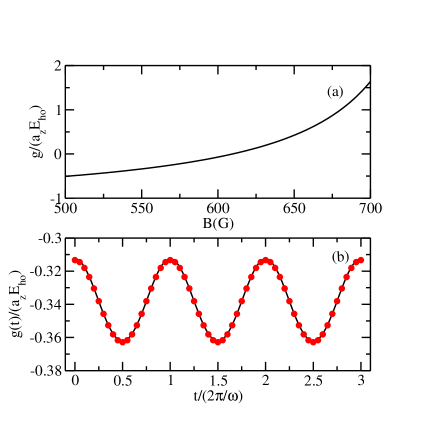
Figure 1: (Color online) Panel (a) shows the 1D coupling constant $g$ as a function of the magnetic field $B$, calculated using Eqs. (4) and (5). Panel (b) shows $g(t)$ as a function of time for an oscillating magnetic field $B(t)=\bar{B}+b\cos(\omega t)$ with $\bar{B}=550\,$G and $b=6\,$G. The solid line is calculated from Eqs. (4)-(7). The dots are calculated from the first order expansion given in Eq. (8).

To test the validity of the approximations in Eq. (8) and (10) in the experimentally relevant regimes, we consider two hyperfine states of ⁶Li, referred to as $|2\rangle=|F=1/2,m_{F}=-1/2\rangle$ and $|3\rangle=|F=3/2,m_{F}=-3/2\rangle$ as an example. We consider the trapping frequencies implemented in Ref. Wenz et al. (2013), i.e. $\omega_{\rho}=2\pi\times 14.22(0.35)$ kHz and $a_{z}=2\pi\times 1.488(0.014)$ kHz. The solid line in Fig. 1(a) shows the 1D coupling constant $g$ as a function of the magnetic field $B$, calculating using Eq. (4) and (5) with $a_{\text{bg}}$, $B_{0}$, and $\Delta$ adapted from Ref. Zürn et al. (2013b). We note that the solid line differs slightly from the the experimentally determined grey curve shown in Figure S3 of Ref. Wenz et al. (2013). This is partly due to the trap calibration and other nearby resonances. A detailed analysis of trap calibration is provided in Ref. Gharashi and Blume (2015). The small difference between the solid line in Fig. 1(a) and the one measured from the experiments does not affect the analysis of the validity regime of approximations in Eq. (8) and (10). A quantitative comparison of the results of this paper and future experiments will require experimental determination of $\bar{g}$ and $d$ from $\bar{B}$ and $b$ instead of using Eqs. (4) and (5) directly.

Figure 1(b) shows the time-dependent coupling constant $g(t)$ resulting from the time-dependent magnetic field in Eq. (7) with $\bar{B}=550\,$G and $b=6\,$G. For this choice of parameters, the first order approximation to $g(t)$ in Eq. (8) is accurate to within 3%. The comparison shows that the first order expansion provides an excellent description of the time dependence of $g(t)$ in the weakly-interacting regime. Equation (8) still works reasonably well even if the interaction energy is comparable to the scale defined by the trap, i.e, $g(t)$ is comparable to $a_{z}E_{\text{ho}}$. For oscillating magnetic field with $\bar{B}=680G$ and $b=4G$, $g(t)$ is averaged at $0.99a_{z}E_{\text{ho}}$ and oscillates between $1.09a_{z}E_{\text{ho}}$ and $0.89a_{z}E_{\text{ho}}$. In this case, the difference between the first order expansion and the exact result is less than $5\%$ of the oscillating magnitude $d$. Similarly, we examine the validity regime of the expansion in the $\bar{g}\rightarrow\infty$ limit by comparing $1/g(t)$ obtained from the first order expansion given in Eq. (10) and the exact result calculated from Eq. (4)-(7). We find that the first order expansion differs from the exact result by less than $1\%$ for $b<1.5G$.

We solve the time-dependent problem using the standard Floquet formalism Shirley (1965); Eckardt and Anisimovas (2015). We rearrange the Hamiltonian in Eq. (2) into two parts,

$$H=H_{0}+H^{\prime}(t),$$ (12)

where $H_{0}$ is time-independent and the time-dependent part is contained in $H^{\prime}(t)$. In the non-interacting limit, $H_{0}$ is given by the first two terms in Eq. (2). In the weakly-interacting regime, $H_{0}$ has an additional contribution from the time-independent part of the two-body coupling

$$V_{2b,0}(z_{j0})=\bar{g}\delta(z_{j}-z_{0}).$$ (13)

In both the $\bar{g}\rightarrow 0$ limit and the weakly-interacting regime, the time-dependent part of the Hamiltonian is

$$H^{\prime}(t)=\sum_{j=1}^{N}d\delta(z_{j}-z_{0})\cos(\omega t).$$ (14)

Following Ref. Volosniev et al. (2014); Levinsen et al. (2015); Gharashi et al. (2015), we treat the $\bar{g}\rightarrow\infty$ limit by replacing the $\delta$-function interaction in Eq. (2) with a set of boundary conditions enforced on the wave function $\Phi$ for (1,1) or (2,1) systems,

$$\left(\frac{\partial\Phi}{\partial z_{j0}}\bigg{|}_{z_{j0}\rightarrow 0^{+}}-\frac{\partial\Phi}{\partial z_{j0}}\bigg{|}_{z_{j0}\rightarrow 0^{-}}\right)=\frac{gm}{\hbar^{2}}\Phi|_{z_{j0}\rightarrow 0}.$$ (15)

$H^{\prime}(t)$ can be written as

$$H^{\prime}(t)=h\cos(\omega t)\mathcal{C},$$ (16)

where $\mathcal{C}$ is the contact density operator. The matrix elements of $\mathcal{C}$ can be obtained using the Hellmann-Feynman theorem with Eq. (15) Volosniev et al. (2014); Gharashi et al. (2015). They are given in Eq. (13) of Ref. Gharashi et al. (2015).

The (2,1) system is degenerate in the limits $\bar{g}\rightarrow 0$ and $\bar{g}\rightarrow\infty$.  Volosniev et al. (2014); Gharashi et al. (2015). In each degenerate manifold, we choose the states whose eigenvalues are smoothly connected to the non-degenerate eigenvalues of the weakly perturbed system. These “good” eigenstates are obtained in the $\bar{g}\rightarrow 0$ limit by applying a small perturbation given in Eq. (13) and in the $\bar{g}\rightarrow\infty$ limit by applying the perturbative boundary condition given in Eq. (15) to the degenerate manifolds.

We construct the Hermitian operator

$$\mathcal{H}=H_{0}+H^{\prime}(t)-i\hbar\frac{\partial}{\partial t}$$ (17)

and find the eigenvalues $\epsilon_{n}$ and the eigenfunctions $|u_{n}(t)\rangle$ of the Hermitian operator $\mathcal{H}$ that satisfy

$$\mathcal{H}|u_{n}(t)\rangle=\epsilon_{n}|u_{n}(t)\rangle.$$ (18)

The eigenfunctions $|u_{n}(t)\rangle$ are called Floquet modes and are periodic in time

$$|u_{n}(t+T)\rangle=|u_{n}(t)\rangle,$$ (19)

where $T=2\pi/\omega$ is the period. The time evolution of an arbitrary state $|\Psi(t)\rangle$ can therefore be written as

$$|\Psi(t)\rangle=\sum_{n}c_{n}\exp(-i\epsilon_{n}t)|u_{n}(t)\rangle,$$ (20)

where the expansion coefficients $c_{n}$ are determined by the initial condition.

The Hilbert space of $\mathcal{H}$ can be expressed as the product space $\mathcal{R}\otimes\mathcal{T}$, where $\mathcal{R}$ is the Hilbert space of $H_{0}$ and $\mathcal{T}$ is the space of functions of periodicity $T$. A complete basis for $\mathcal{H}$ is formed from the product states $|\psi_{n}\rangle\otimes|l\rangle$, where $|\psi_{n}\rangle$ are the eigenstates of $H_{0}$ and $\langle t|l\rangle=\exp(il\omega t)$. Here, $l$ is an integer quantum number that labels the “Floquet band”. For systems considered in this work, the center-of-mass motion separates from the relative motion and its time-dependence is trivial because it is governed by a time-independent Hamiltonian. We hence focus on the relative degrees of freedom and assume that the center-of-mass motion is always in its ground state. For trapped (1,1) system, the exact solution for arbitrary interaction strength is given in Ref. Busch et al. (1998). We use the exact solution combined with the time period functions as our basis functions. For the trapped (2,1) system, the exact solutions for the $\bar{g}\rightarrow 0$ limit and the $\bar{g}\rightarrow\infty$ limit are known Volosniev et al. (2014). For the weakly-interacting regime, we use the exact solution for the $\bar{g}\rightarrow 0$ limit combined with the time period functions as our basis functions. In this work, we use about 100 basis functions for the time-independent Hamiltonian and consider about 200 Floquet bands, corresponding to a total of 20,000 basis functions for the time-dependent problem. We have tested to make sure that all our results remain unchanged if the basis set is further enlarged.

III Results

III.1 $\bar{g}\rightarrow 0$ limit

In the $\bar{g}\rightarrow 0$ limit, the relative eigenstates of the (1,1) system for the time-independent part of the Hamiltonian $H_{0}$ are the harmonic oscillator eigenstates $\psi_{q}(z)=N_{q}\exp(-z^{2}/(4a_{z}^{2}))H_{2q}(z/(\sqrt{2}a_{z}))$, with eigenenergies $E_{q}=(2q+1/2)\hbar\omega_{z}$. Here, $z=z_{1}-z_{0}$ is the relative coordinate, $N_{q}$ is a normalization constant, and $H_{n}$ denotes the $n$-th Hermite polynomial. The even-parity states are labeled by integers $q=0,1,2,\ldots$ and are coupled by the time-dependent, zero-range interactions. The energy spacing between two consecutive even-parity eigenstates is $2\hbar\omega$. The odd-parity states, labeled by half integers $q=1/2,3/2,\ldots$, are not affected by the zero-range interaction since the wave functions have zero amplitude at $z=0$. Therefore, the odd-parity states will not be populated during the time evolution. A small portion of the energy spectrum for the (1,1) system near the $\bar{g}\rightarrow 0$ limit is shown in Figure 2(d). Solid, dashed, dotted and dash-dotted lines show the eigenenergies of the even parity states with $q=0,1,2$, and $3$, respectively, as a function of $g/(a_{z}E_{\text{ho}})$, in the $\bar{g}\rightarrow 0$ limit. even-parity states, whose eigenenergies remain constants for different $g$, are not shown in the figure.

We prepare the system in the ground state $\psi_{0}(z)$ and time evolve the system under the Hamiltonian given in Eq. (12). The driving frequency $\omega$ is chosen to be on or near resonance with the energy spacing between the ground state and the first excited even-parity state $\psi_{1}(z)$. We calculate the probability of occupying the even-parity states $\psi_{q}(z)$ as a function of time. We find that in the weak driving limit, which in practice translates to $d/(a_{z}E_{\text{ho}})<0.2$, the time dynamics is approximately invariant for different $d$ if we correspondingly scale the time by $2\pi\hbar a_{z}/d$. This motivates us to define a scaled dimensionless time $\tau=t/(2\pi\hbar a_{z}/d)$. In this way, the dynamics we obtained in terms of $\tau$ applies to all driving strengths $d$ in the range $d/(a_{z}E_{\text{ho}})<0.2$. In the two-state model, this invariance is a consequence of the validity of the first-order rotating wave approximation Wang and Sun (1996). Our observation for the non-interacting (1,1) system is consistent with the two-state case, and is also found to be true for other systems and other regimes discussed in this work.

Figure 2(a) shows the probability of occupying different even-parity states as a function of $\tau$ when the driving is on resonance, i.e. $\omega=2\omega_{z}$. We find that not only is the $q=1$ state populated, but higher-$q$ states are in turn populated with significant probability. The probability of the populated states revives on the time scale set by $2\pi\hbar a_{z}/d$, which is much longer than the driving period $T$. The probability of the ground state and the first excited states are, on average, the highest among all states and the pattern of the revival dynamics roughly repeats itself in the long time limit. Figures 2(b) and (c) show the same quantity when the driving is slightly off-resonance, i.e. $\omega=2\omega_{z}+\delta$, where $\delta$ is the detuning. The dynamics is invariant for different choices of $d$ when the detuning $\delta$ is scaled by $d/(\hbar a_{z})$ under the condition $\delta\ll\omega_{z}$. For example, the dynamics for the case shown in Fig. 2(c) with $d=0.01a_{z}E_{\text{ho}}$ and $\delta=0.003\omega_{z}$ is almost the same as for $d=0.1a_{z}E_{\text{ho}}$ and $\delta=0.03\omega_{z}$. The detuning suppresses the transition from the ground state to the excited states and the suppression is stronger for higher energy states. As the detuning increases, the system gradually becomes an effective two-state system where the probability of occupying higher excited states becomes negligible. The dynamics shown in Fig. 2(c) is very similar to the case where only the $q=0$ and $1$ states are considered.

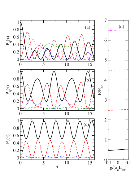
Figure 2: (Color online) Dynamics of the (1,1) system under oscillating magnetic field in the $\bar{g}\rightarrow 0$ limit. The driving strength is $d=0.01a_{z}E_{\text{ho}}$ for all cases. The figures remain almost unchanged for different driving strength $d$ for $d<0.2a_{z}E_{\text{ho}}$. Panel (a) shows the on-resonance case where $\omega=2\omega_{z}$. The solid, dashed, dotted, dash-dotted and dash-dot-dotted lines show the probability $P_{q}(\tau)$ of occupying the state with $q=0$, 1, 2, 3 and any other state as functions of the scaled dimensionless time $\tau=t/(2\pi\hbar a_{z}/d)$. Panel (b) and (c) show the slightly off-resonance cases, where the detunings $\delta$ are $0.15d/(\hbar a_{z})$ and $0.3d/(\hbar a_{z})$, respectively. The solid, dashed, dotted, and dash-dot-dotted lines show $P_{q}(\tau)$ for $q=0$, 1, 2, and any other state as a function of $\tau$. Panel (d) shows the energy spectrum of (1,1) system near the $\bar{g}\rightarrow 0$ limit for even-parity states. The solid, dashed, dotted, and dash-dotted lines show the energy of the four lowest states as a function of $g/(a_{z}E_{\text{ho}})$, which are labeled by $q=0$, 1, 2, and 3.

The ground state of (2,1) system has odd relative parity. Since the zero-range interactions conserve the relative parity, the even-parity states will not be populated if we initially prepare the state in the ground state. Hence, we consider only odd-parity states. We note that, among the odd-parity states, some are not affected by zero-range interaction. Unlike the (1,1) system, degeneracy exists for the excited states and is lifted in the presence of interaction. The energy of the lowest relative eigenstate is $2\hbar\omega_{z}$. There are two odd-parity states with energy $4\hbar\omega_{z}$. Only one of these is affected by the zero-range interaction. There are three odd-parity states with energy $6\hbar\omega_{z}$, of which two states are affected by the zero-range interaction. A small portion of the energy spectrum for the (2,1) system near the $\bar{g}\rightarrow 0$ limit is shown in Fig. 3(d). Solid, dashed, dotted and dash-dotted lines show the eigenenergies of odd-parity states with $E/E_{\text{ho}}=2,4,6$, and $6$, respectively, as a function of $g/(a_{z}E_{\text{ho}})$ in the $\bar{g}\rightarrow 0$ limit. The states that are not affected by the zero-range interactions are not shown. As explained in Sec. II, the two degenerate states with eigenenergy $6\hbar\omega_{z}$ in the $\bar{g}\rightarrow 0$ limit are good eigenstates that change smoothly when deviating from the $\bar{g}\rightarrow 0$ limit.

Figure 3 shows the probability of occupying different odd-parity states as a function of scaled dimensionless time $\tau$ for the (2,1) system. When the driving is on resonance, i.e. $\omega=2\omega_{z}$, the dynamics is notably different from the (1,1) system as the revival is much weaker in the (2,1) system. However, as the detuning increases, the transition to high excited states is suppressed. As a result, the revival dynamics of the two lowest states start to appear. Similar to the (1,1) system, higher detuning gradually leads to an effective two-state system as the transition to higher excited states is further suppressed.

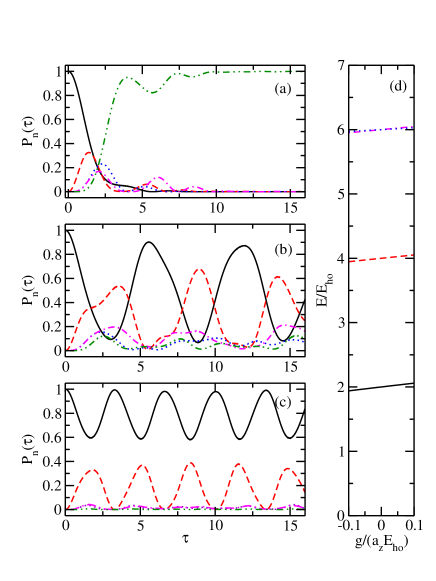
Figure 3: (Color online) Dynamics of the (2,1) system under oscillating magnetic field in the $\bar{g}\rightarrow 0$ limit. The driving strength is $d=0.01a_{z}E_{\text{ho}}$ for all cases. The figures remains almost unchanged for different driving strength $d$ for $d<0.2a_{z}E_{\text{ho}}$. Panel (a) shows the on-resonance case where $\omega=2\omega_{z}$. The solid, dashed, dotted, dash-dotted and dash-dot-dotted lines show the probability $P_{n}(t)$ of occupying the odd-parity states with relative eigenenergies $E_{n}/\hbar\omega_{z}=2$, $4$, $6$, $6$, and any other state as functions of the scaled dimensionless time $\tau=t/(2\pi\hbar a_{z}/d)$. Note that there are two degenerate states with $E_{n}/\hbar\omega_{z}=6$ that are affected by the zero-range interaction in the $\bar{g}\rightarrow 0$ limit. Panel (b) and (c) show the slightly off-resonance cases, where the detunings $\delta$ are $0.15d/(\hbar a_{z})$ and $0.3d/(\hbar a_{z})$, respectively. The solid, dashed, dotted, dash-dotted, and dash-dot-dotted lines show the probability $P_{n}(t)$ of occupying the state with $E_{n}/\hbar\omega_{z}=2$, $4$, $6$, $6$, and any other state as functions of $\tau$. Panel (d) shows the energy spectrum of the (2,1) system near $\bar{g}\rightarrow 0$ limit for states with odd relative parity. The solid, dashed, dotted, and dash-dotted lines show the states with relative eigenenergies $E_{n}/\hbar\omega_{z}=2$, $4$, $6$, and $6$. Please note that the dotted and dash-dotted lines are very close to each other. There are one and two additional states with $E_{n}/\hbar\omega_{z}=4$ and $6$, respectively, that are not affected by the interaction and are not shown in the figure.

III.2 Weakly-interacting regime

As the system moves away from the $\bar{g}\rightarrow 0$ limit, the energy spacing between two consecutive states of the (1,1) system is no longer $2\hbar\omega_{z}$. The relative eigenstates with even-parity for the time-independent Hamiltonian $H_{0}$ become $\psi_{q}(z)=N_{q}\exp(-z^{2}/(4a_{z}^{2}))U(-q,1/2,z^{2}/(2a_{z}^{2}))$ with eigenenergies $E_{q}=(2q+1/2)\hbar\omega_{z}$, for non-integer $q$. Here, $N_{q}$ is a normalization constant and $U$ denotes the confluent hypergeometric function. The non-integer quantum number $q$ is determined by the transcendental equation Busch et al. (1998)

$$\frac{2\Gamma(-q+1/2)}{\Gamma(-q)}=-\frac{\bar{g}}{\sqrt{2}a_{z}\hbar\omega_{z}}.$$ (21)

The odd-parity states remain unaffected by the zero-range interaction.

As in the $\bar{g}\rightarrow 0$ case, we prepare the system in the ground state. We first consider an example case where $\bar{g}=-0.1a_{z}E_{\text{ho}}$ and $d=0.02a_{z}E_{\text{ho}}$. Since the interaction is weak and attractive, the energies of the relative eigenstates are shifted down slightly compared to the $\bar{g}\rightarrow 0$ case. The energies of the three lowest states with even-parity are $0.459\hbar\omega_{z}$, $2.480\hbar\omega_{z}$, and $4.485\hbar\omega_{z}$, respectively, giving spacings $2.021\hbar\omega_{z}$ and $2.005\hbar\omega_{z}$, respectively. The three lowest states are shown as solid, dashed, and dotted lines, respectively, in Fig. 4(c). We choose the driving frequency to be on resonance with the energy difference between the ground state and the lowest excited state with even parity, i.e. $\omega=2.021\omega_{z}$. The difference in energy spacing between consecutive even-parity states greatly suppresses the transition to higher excited states. As a result, the system is accurately described by a two-state Rabi oscillation. Figure 4(a) shows the dynamics of the case discussed above. The probability of occupying the states besides the two states in Rabi oscillation is less than $2\%$. This observation is similar to the three-dimensional system considered in Ref. Bertelsen and Mølmer (2006).

Stronger interaction (greater $\bar{g}$) or weaker driving (smaller $d$) suppress the transition to higher excited states, resulting in a more ideal two-state model. With weaker interaction or stronger driving, the transition to the higher excited states becomes non-negligible. We find that the dynamics of the weakly-interacting system remains almost invariant for the same $\bar{g}/d$, e.g. the dynamics for a case with $\bar{g}=-0.2a_{z}E_{\text{ho}}$ and $d=0.04a_{z}E_{\text{ho}}$ is almost identical to the case shown in Fig. 4(a). The applicability of the two-state model can be assessed through the maximum probability of occupying any state other than the two states in the Rabi oscillation $P_{\text{other}}$, which are shown in Figure 4(b) for a range of average coupling constant $\bar{g}/d$. The system can be described by a two-state model fairly well in the $|\bar{g}|/d\gtrsim 2.5$ regime, where $P_{\text{other}}$ is less than 10%. Besides the transition from the ground state to first excited state, we checked that the two-state model is also applicable when driving a transition from the ground state to other excited states. The validity regime of the two-state model is greater for higher excited states. For example, the transition from the ground state to the fourth excited state and tenth excited state can be described by a two-state model in the regime $|\bar{g}|/d\gtrsim 1.0$ and $|\bar{g}|/d\gtrsim 0.7$, respectively.

As shown above, the oscillating magnetic field can drive the system from the ground state to an excited state with near-unity probability for a wide range of parameter combinations. In cold atom experiments, the excited state could be populated by the following scheme. 1. Prepare the system in the $\bar{g}\rightarrow 0$ limit ($\bar{g}\rightarrow 0^{+}$). 2. Tune the interaction strength to a small but non-zero positive value of $\bar{g}$ adiabatically through the CIR. 3. Turn on the oscillating magnetic field, with the driving frequency matching the energy difference between the ground state and the excited state. The driving strength $d$ should be chosen according to the guideline discussed above. Once the excited state is populated, the system could be tuned further into a strongly-interacting regime adiabatically through CIR.

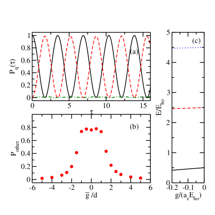
Figure 4: (Color online) Dynamics of the (1,1) system under an oscillating magnetic field in the weakly-interacting regime. Panel (a) shows the case where $\bar{g}=-0.1a_{z}E_{\text{ho}}$ and $d=0.02a_{z}E_{\text{ho}}$. The dynamics remains almost the same for different values of $\bar{g}$ and $d$ giving the same $\bar{g}/d$. Solid, dashed and dash-dotted lines show the probability $P_{q}(t)$ of occupying the ground state, the lowest excited state with even parity, and any other state as a function of the scaled dimensionless time $\tau=t/(2\pi\hbar a_{z}/d)$. Panel (b) shows the applicability of the two-state model. Circles show the maximum probability of occupying any state other than the two states in the Rabi oscillation $P_{\text{other}}$ as a function of $\bar{g}/d$. Panel (c) shows the energy spectrum of the (1,1) system near $\bar{g}=-0.1a_{z}E_{\text{ho}}$ for even-parity states. Solid, dashed, and dotted lines show the energy of the three lowest states with even parity.

For the interacting (2,1) system, the degeneracy of the excited states in the $\bar{g}\rightarrow 0$ limit is partly broken. Some of the states within the degenerate manifold in the $\bar{g}\rightarrow 0$ limit become near-degenerate states in the weakly-interacting regime. For instance, there are four odd-parity states with relative energy $8\hbar\omega_{z}$ in the $\bar{g}\rightarrow 0$ limit. One of the four states is not affected by the zero-range interaction while the other three are slightly shifted down by the weak attractive interaction. For $\bar{g}=-0.08a_{z}E_{\text{ho}}$, the energies of the three shifted states become $7.9620\hbar\omega_{z}$, $7.9764\hbar\omega_{z}$, and $7.9833\hbar\omega_{z}$, respectively, giving energy spacings $0.0144\hbar\omega_{z}$ and $0.0069\hbar\omega_{z}$. We note that the energy difference between the two latter states, denoted here as $|\psi_{a}\rangle$ and $|\psi_{b}\rangle$, is very small compared to $\hbar\omega_{z}$. The on-resonance driving frequency from the ground state ($1.9516\hbar\omega_{z}$) to $|\psi_{a}\rangle$ and $|\psi_{b}\rangle$ are $6.0247\omega_{z}$ and $6.0316\omega_{z}$, respectively. The ground state, $|\psi_{b}\rangle$, and $|\psi_{a}\rangle$ are shown as solid, dashed, and dotted lines, respectively, in Fig. 5(d). Other odd-parity states that are affected by the zero-range interactions are shown as dash-dotted lines. In this case, we will demonstrate that it is possible to design a tunable effective three-state model by choosing a driving frequency that lies between the two on-resonance driving frequencies. We remark that the driving between the ground state and the two former states in the near degenerate manifold does not yield an ideal three-state model as the case shown here since the energy spacing is larger.

Figure 5 shows the dynamics of the (2,1) system in the parameter combination discussed above. Solid, dashed, dotted and dash-dotted lines show the probability of occupying the ground state, $|\psi_{b}\rangle$, $|\psi_{a}\rangle$, and all other odd-parity states as a function of time. Panel (a) shows the case where the driving frequency $\omega$ is on resonance with the energy difference between the ground state and $|\psi_{b}\rangle$, i.e. $\omega=6.0316\omega_{z}$. In this case, the system can be described very well by a two-state Rabi oscillation between the ground state and $|\psi_{b}\rangle$. Panel (b) and (c) show the cases where the driving frequencies are $\omega=6.0266\omega_{z}$ and $6.0251\omega_{z}$, respectively. In both cases, the ground state, $|\psi_{a}\rangle$ and $|\psi_{b}\rangle$ are populated with significant probability. The relative probability between $|\psi_{a}\rangle$ and $|\psi_{b}\rangle$ can be tuned, within a certain range, by tuning the driving frequency. The tunable effective three-state model could potentially be used as a building block for the realization of quantum Potts model in cold atom systems if multiple trapped (2,1) systems are prepared and coupled together Messio et al. (2013).

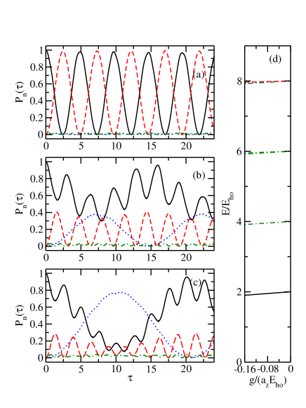
Figure 5: (Color online) Dynamics of the (2,1) system under an oscillating magnetic field in the weakly-interacting limit. The average coupling constant is $\bar{g}=-0.08a_{z}E_{\text{ho}}$, and the driving strength is $d=0.02a_{z}E_{\text{ho}}$. Panel (a), (b), and (c) show cases with driving frequency $\omega=6.0316\omega_{z}$, $6.0266\omega_{z}$ and $6.0251\omega_{z}$, respectively. Solid, dashed, dotted, and dash-dotted lines show the probability $P_{q}(\tau)$ of occupying the ground state, $|\psi_{b}\rangle$, $|\psi_{a}\rangle$, and any other state as functions of the scaled dimensionless time $\tau=t/(2\pi\hbar a_{z}/d)$. See text for details. Panel (d) shows the energy spectrum of the (2,1) system near $\bar{g}=-0.08a_{z}E_{\text{ho}}$ for states with odd parity. The solid, dashed, and dotted lines show the energy of ground state, $|\psi_{b}\rangle$, and $|\psi_{a}\rangle$, respectively. The rest of the states are represented by dash-dotted lines. Please note that the dashed and dotted lines are very close to each other. The states not affected by the zero-range interactions are not shown in the figure.

III.3 $\bar{g}\rightarrow\infty$ limit

In the $\bar{g}\rightarrow\infty$ limit, the non-integer quantum number $q$ for the even-parity states of the (1,1) system takes half integer values $q=1/2,3/2,\ldots$ and the eigenenergies are given by $E_{q}=(2q+1/2)\hbar\omega_{z}$. Hence, the even-parity states becomes degenerate with the odd-parity states which are not affected by the zero-range interaction. Figure 6(d) shows a small portion of the energy spectrum for the (1,1) system near the $\bar{g}\rightarrow\infty$ limit. The odd-parity states are not shown in the figure.

We prepare the system in the lowest state with even parity and let the system evolve under the Hamiltonian given in Eqs. (12) and (16). We first set the driving frequency to be on resonance with the energy difference between the two lowest states with even parity, i.e. $\omega=2\omega_{z}$. We find that as the system evolves in time, every even-parity state in turn gets excited and then depleted. Similar to the $\bar{g}\rightarrow 0$ limit and the weakly-interacting regime, the dynamics of the system is almost invariant for different driving strengths $h$ if we scale the time $t$ by $2\pi/(ha_{z}\hbar\omega_{z}^{2})$. Hence, in the $\bar{g}\rightarrow\infty$ limit, we define the scaled dimensionless time $\tau=t/(2\pi/(ha_{z}\hbar\omega_{z}^{2}))$. Solid lines in Figure 6(a) show the probability of occupying the 12 lowest eigenstates as a function of $\tau$. We find that the eigenstates with larger $q$ quantum number peak at longer times $\tau_{q}$. Figure 6(b) shows the scaled peaking time $\tau_{q}$ of an eigenstate as a function of the square root of the quantum number $\sqrt{q}$. We find that $\tau_{q}$ scales linearly with $\sqrt{q}$. A two parameter fit yields $\tau_{q}=-0.036(2)+0.178(1)\sqrt{q}$. Figure 6(c) shows the peak probability $P_{q}(\tau_{q})$ as a function of $1/\sqrt{q}$. We find that the peak probability is inversely proportional to $\sqrt{q}$. A two parameter fit shows an absence of constant term within numerical accuracy and hence $P_{q}(\tau_{q})=0.435(1)/\sqrt{q}$. We emphasize here that the two relations shown here are applicable in the weak driving regime, which translates to $h<0.05/(a_{z}E_{\text{ho}})$. The two relations show that the energy is being continuously pumped into the system through the oscillating magnetic field and the coupling to higher excited states is unbounded. The energy transfer between states in an open quantum system is a topic of great interest Roden and Whaley (2016). The system we considered is a specific example that could be analyzed through the general framework in Ref. Roden and Whaley (2016) using the quantum master equation.

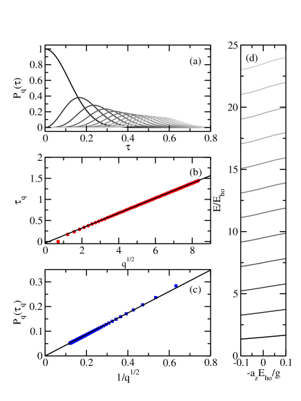
Figure 6: (Color online) Dynamics of the (1,1) system under an oscillating magnetic field in the $\bar{g}\rightarrow\infty$ limit. The driving strength is $h=0.002/(a_{z}E_{\text{ho}})$. The driving frequency is $\omega=2\omega_{z}$. The solid lines in panel (a) show the probabilities $P_{q}(\tau)$ of occupying 12 lowest eigenstates as functions of the scaled dimensionless time $\tau=t/(2\pi/(ha_{z}\hbar\omega_{z}^{2}))$. The eigenstates with quantum number $q=1/2$, $3/2$, $\ldots$ are shown successively by solid lines with darker grey (peaking at a shorter time) to lighter grey (peaking at a longer time). Circles in panel (b) show the scaled peaking time $\tau_{q}$ as a function of $\sqrt{q}$. Squares in panel (c) show the peak probability $P_{q}(\tau_{q})$ as a function of $1/\sqrt{q}$. The lines in panel (b) and (c) are linear fits. Panel (d) shows the energy spectrum for the (1,1) system near the $\bar{g}\rightarrow\infty$ limit. The states with lower (higher) energies are shown by solid lines with darker (lighter) grey.

The unbounded coupling is only present when the driving frequency is exactly on resonance. When the driving is slightly off resonance, i.e., the detuning $\delta$ is non-zero, the revival of the ground state occurs on a time scale determined by the detuning. Figure 7(a) shows the dynamics of the (1,1) system at $\bar{g}\rightarrow\infty$ under oscillating magnetic field with a driving frequency of $\omega=1.998\omega_{z}$, where the detuning is $\delta=1.0ha_{z}\hbar\omega_{z}^{2}$. The number of excited states that are populated is limited compared to the on-resonance case. The probability of the ground state revives after a certain time $\bar{\tau}$ to near unity. The revival dynamics repeats itself in a period of $\bar{\tau}$ in the long time limit. We calculated the revival period $\bar{\tau}$ for different scaled detuning $\delta/(ha_{z}\hbar\omega_{z}^{2})$. Figure 7(b) shows the inverse revival period $1/\bar{\tau}$ as a function of scaled detuning $\delta/(ha_{z}\hbar\omega_{z}^{2})$. We find that the revival period is inversely proportional to the absolute value of the scaled detuning strength and the proportionality factor is 1 within numerical accuracy as determined from a fit, i.e, our numerics suggests that $\bar{\tau}=ha_{z}\hbar\omega_{z}^{2}/|\delta|$. If we express this relation in terms of unscaled revival period $T_{\text{rev}}$, we find $T_{\text{rev}}=2\pi/|\delta|$.

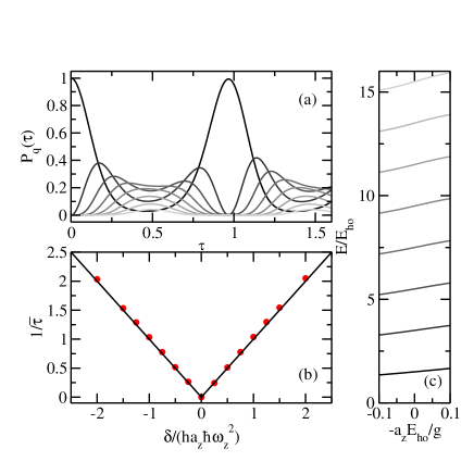
Figure 7: (Color online) Dynamics of the (1,1) system under oscillating magnetic field in the $\bar{g}\rightarrow\infty$ limit. The driving strength is $h=0.002/(a_{z}E_{\text{ho}})$. Panel (a) shows the case of near-resonant driving frequency $\omega=1.998\omega_{z}$. The detuning is $\delta=1.0ha_{z}\hbar\omega_{z}^{2}$. Solid lines show the probability of occupying the 8 lowest eigenstates as a function of the scaled time $\tau=t/(2\pi/(ha_{z}\hbar\omega_{z}^{2}))$. The eigenstates with quantum number $q=1/2$, $3/2$, $\ldots$ are shown successively by solid lines with darker to lighter grey. Panel (b) shows the inverse revival period $1/\bar{\tau}$ for the ground state as a function of scaled detuning $\delta/(ha_{z}\hbar\omega_{z}^{2})$. The solid line shows $1/\bar{\tau}=|\delta|/(ha_{z}\hbar\omega_{z}^{2})$. Panel (c) shows the energy spectrum for the (1,1) system near the $\bar{g}\rightarrow\infty$ limit. The states with lower (higher) energies are shown by solid lines with darker (lighter) grey.

In the $\bar{g}\rightarrow\infty$ limit, the dynamics of the (2,1) system is very similar to the (1,1) system. When the driving is on resonance, i.e. $\omega=2\omega_{z}$, we observe similar unbounded coupling as in the (1,1) system. Although the excited states of the (2,1) system at $\bar{g}\rightarrow\infty$ limit are degenerate, only one good eigenstate within each degenerate manifold can be populated with significant probability as time evolves. Similar to the (1,1) system, the scaled peaking time $\tau_{n}$ and the peak probability $P_{n}(\tau_{n})$ are linearly proportional and reversely proportional to the square root of eigenenergy $\sqrt{E_{n}}$, respectively. Our fits yield $\tau_{n}=-0.10(2)+0.090(2)\sqrt{E_{n}/E_{\text{ho}}}$ and $P_{n}(\tau_{n})=-0.06(1)+0.92(1)/\sqrt{E_{n}/E_{\text{ho}}}$. The detuning has exactly the same effect on the dynamics as in the (1,1) system. The relation between the revival period and detuning discovered in the (1,1) system still holds for the (2,1) system.

IV Conclusion and Outlook

This paper studied the dynamics of a harmonically trapped two- and three-fermion systems under an oscillating magnetic field. Previous works have studied the quantum dynamics of periodically driven one- and two-state systems. The systems considered in this work are considerably more complicated. Yet, they represent the simplest realistic few-body systems that have been successfully prepared in experiments. Therefore, the dynamics studied in this work could be investigated using existing experimental setups. We analyzed these systems in the non-interacting limit, weakly-interacting regime and the $\bar{g}\rightarrow\infty$ limit, and we related these regimes to the parameter regimes that are accessible in the experiments.

We found that the dynamics of the systems studied contains rich physics. We revealed the dynamic difference in the the revival dynamics between the (1,1) and (2,1) systems in the non-interacting limit. We determined the parameter regimes where the two-state Rabi oscillation model is applicable and a population transfer with near-unity probability can potentially be realized in the experiments. We also designed a tunable three-state model in the (2,1) system. Moreover, we found an unbounded coupling to all excited states in the $\bar{g}\rightarrow\infty$ limit when the driving is on resonance in both (1,1) and (2,1) systems. We discovered the relation between the peak probability, peaking time, and the eigenenergy for all states.

Following the success in preparing few-body cold atom systems in the experiments, there has been increasing interest in the dynamics of time-dependent few-body systems. Studies have been performed on the dynamics of a cold atom system after a rapid change of scattering length Corson and Bohn (2016) and a displacement of the trap Streltsova et al. (2014). Methods for state-transfer engineering have been proposed in cold atom systems Martínez-Garaot et al. (2015). There are also studies on dynamics for cold atom systems in a time-dependent trapping potential Deng et al. (2016); Ebert et al. (2016); Gharashi and Blume . Our study, which focuses on the dynamics induced by the time-dependent interactions, belongs to the broader literature of few-body dynamics.

One of the key results in this work closely related to the experiments is that population transfer between states with near-unity probability can be achieved in the weakly-interacting regime. The reason is that the interaction breaks the equal-energy spacing between eigenstates. Similar effects can be generated by slightly deforming the trap, e.g. adding a term proportional to $z^{4}$ to the trapping potential. At the same time, the time-dependent driving could also be introduced by modulating confinement instead of the interaction. Although such methods may introduce coupling between the center-of-mass motion and the relative motion, the effect of coupling may be negligible in some parameter regimes. These alternative techniques are worth investigating since they provide more flexibility for the future experiments.

The additional energy scales introduced by the periodic driving open up new possibilities in cold atom research. The few-body systems studied in this work could potentially be coupled to form a lattice. The coupling of an array of effective two-state and three-state systems could lead to new proposals in quantum computing. Recently, there has been a proposal to use cold atoms in shaking harmonic traps to implement synthetic dimensions Price et al. and a realization of spin-orbit coupling through a time-modulated magnetic field gradient Luo et al. (2016). In those works, a single-particle picture for each harmonic trap is considered. Our work shows that interactions between atoms can have an important impact on the dynamics. Our results for the few-body systems can serve as input for the coupled many-body systems in future studies.

V Acknowledgement

X. Y. Y. is supported by NSF Grant DMR-1309615, MURI Grant FP054294-D, and NASA Fundamental Physics Grant 1518233. Y. Y. is supported by NSF Grant PHY-1415112. X. Y. Y. thanks T.-L. Ho for useful discussions. We are grateful to D. Blume for careful reading of the manuscript and thoughtful comments.

References

- Serwane et al. (2011) F. Serwane, G. Zürn, T. Lompe, T. B. Ottenstein, A. N. Wenz, and S. Jochim, “Deterministic preparation of a tunable few-fermion system,” Science 332, 336 (2011).
- Wenz et al. (2013) A. N. Wenz, G. Zürn, S. Murmann, I. Brouzos, T. Lompe, and S. Jochim, “From few to many: Observing the formation of a Fermi sea one atom at a time,” Science 342, 457 (2013).
- Chin et al. (2010) C. Chin, R. Grimm, P. Julienne, and E. Tiesinga, “Feshbach resonances in ultracold gases,” Rev. Mod. Phys. 82, 1225 (2010).
- Olshanii (1998) M. Olshanii, “Atomic scattering in the presence of an external confinement and a gas of impenetrable bosons,” Phys. Rev. Lett. 81, 938 (1998).
- Gharashi and Blume (2013) S. E. Gharashi and D. Blume, “Correlations of the upper branch of 1D harmonically trapped two-component Fermi gases,” Phys. Rev. Lett. 111, 045302 (2013).
- Harshman (2012) N. L. Harshman, “Symmetries of three harmonically trapped particles in one dimension,” Phys. Rev. A 86, 052122 (2012).
- Sowiński et al. (2013) T. Sowiński, T. Grass, O. Dutta, and M. Lewenstein, “Few interacting fermions in a one-dimensional harmonic trap,” Phys. Rev. A 88, 033607 (2013).
- Volosniev et al. (2014) A. G. Volosniev, D. V. Fedorov, A. S. Jensen, M. Valiente, and N. T. Zinner, “Strongly interacting confined quantum systems in one dimension,” Nat Commun 5, 5300 (2014).
- Levinsen et al. (2015) J. Levinsen, P. Massignan, G. M. Bruun, and M. M. Parish, “Strong-coupling ansatz for the one-dimensional Fermi gas in a harmonic potential,” Science Advances 1, e1500197 (2015).
- Zürn et al. (2013a) G. Zürn, A. N. Wenz, S. Murmann, A. Bergschneider, T. Lompe, and S. Jochim, “Pairing in few-fermion systems with attractive interactions,” Phys. Rev. Lett. 111, 175302 (2013a).
- Murmann et al. (2015) S. Murmann, A. Bergschneider, V. M. Klinkhamer, G. Zürn, T. Lompe, and S. Jochim, “Two fermions in a double well: Exploring a fundamental building block of the Hubbard model,” Phys. Rev. Lett. 114, 080402 (2015).
- Dittrich et al. (1998) T. Dittrich, P. Hänggi, G.-L. Ingold, B. Kramer, G. Schön, and W. Zwerger, Quantum transport and dissipation (Wiley-VCH, Weinheim, 1998).
- Eckardt and Anisimovas (2015) A. Eckardt and E. Anisimovas, “High-frequency approximation for periodically driven quantum systems from a Floquet-space perspective,” New Journal of Physics 17, 093039 (2015).
- Goldman and Dalibard (2014) N. Goldman and J. Dalibard, “Periodically driven quantum systems: Effective Hamiltonians and engineered gauge fields,” Phys. Rev. X 4, 031027 (2014).
- Bukov et al. (2015) M. Bukov, L. D’Alessio, and A. Polkovnikov, “Universal high-frequency behavior of periodically driven systems: from dynamical stabilization to Floquet engineering,” Advances in Physics 64, 139 (2015).
- Gharashi et al. (2015) S. E. Gharashi, X. Y. Yin, Y. Yan, and D. Blume, “One-dimensional Fermi gas with a single impurity in a harmonic trap: Perturbative description of the upper branch,” Phys. Rev. A 91, 013620 (2015).
- Thompson et al. (2005) S. T. Thompson, E. Hodby, and C. E. Wieman, “Ultracold molecule production via a resonant oscillating magnetic field,” Phys. Rev. Lett. 95, 190404 (2005).
- Gaebler et al. (2007) J. P. Gaebler, J. T. Stewart, J. L. Bohn, and D. S. Jin, “-wave Feshbach molecules,” Phys. Rev. Lett. 98, 200403 (2007).
- Borca et al. (2003) B. Borca, D. Blume, and C. H. Greene, “A two-atom picture of coherent atom-molecule quantum beats,” New Journal of Physics 5, 111 (2003).
- Bertelsen and Mølmer (2006) J. F. Bertelsen and K. Mølmer, “Molecule formation in optical lattice wells by resonantly modulated magnetic fields,” Phys. Rev. A 73, 013811 (2006).
- Brouard and Plata (2015) S. Brouard and J. Plata, “Feshbach molecule formation through an oscillating magnetic field: subharmonic resonances,” Journal of Physics B: Atomic, Molecular and Optical Physics 48, 065002 (2015).
- Langmack et al. (2015) C. Langmack, D. H. Smith, and E. Braaten, “Association of atoms into universal dimers using an oscillating magnetic field,” Phys. Rev. Lett. 114, 103002 (2015).
- (23) T.-L. Ho and X. Y. Yin, “Energy cascade in quantum gases,” manuscript in preparation .
- Zürn et al. (2013b) G. Zürn, T. Lompe, A. N. Wenz, S. Jochim, P. S. Julienne, and J. M. Hutson, “Precise characterization of Feshbach resonances using trap-sideband-resolved RF spectroscopy of weakly bound molecules,” Phys. Rev. Lett. 110, 135301 (2013b).
- Gharashi and Blume (2015) S. E. Gharashi and D. Blume, “Tunneling dynamics of two interacting one-dimensional particles,” Phys. Rev. A 92, 033629 (2015).
- Shirley (1965) J. H. Shirley, “Solution of the Schrödinger equation with a Hamiltonian periodic in time,” Phys. Rev. 138, B979 (1965).
- Busch et al. (1998) T. Busch, B.-G. Englert, K. Rzażewski, and M. Wilkens, “Two cold atoms in a harmonic trap,” Found. of Phys. 28, 549 (1998).
- Wang and Sun (1996) X.-G. Wang and C.-P. Sun, “Higher-order correction for rotating wave approximation, Rabi transformation, and its applications in the Jaynes-Cummings model,” Acta Physica Sinica 5, 881 (1996).
- Messio et al. (2013) L. Messio, P. Corboz, and F. Mila, “Competition between three-sublattice order and superfluidity in the quantum three-state potts model of ultracold bosons and fermions on a square optical lattice,” Phys. Rev. B 88, 155106 (2013).
- Roden and Whaley (2016) J. J. J. Roden and K. B. Whaley, “Probability-current analysis of energy transport in open quantum systems,” Phys. Rev. E 93, 012128 (2016).
- Corson and Bohn (2016) J. P. Corson and J. L. Bohn, “Ballistic quench-induced correlation waves in ultracold gases,” Phys. Rev. A 94, 023604 (2016).
- Streltsova et al. (2014) O. I. Streltsova, O. E. Alon, L. S. Cederbaum, and A. I. Streltsov, “Generic regimes of quantum many-body dynamics of trapped bosonic systems with strong repulsive interactions,” Phys. Rev. A 89, 061602 (2014).
- Martínez-Garaot et al. (2015) S. Martínez-Garaot, A. Ruschhaupt, J. Gillet, T. Busch, and J. G. Muga, “Fast quasiadiabatic dynamics,” Phys. Rev. A 92, 043406 (2015).
- Deng et al. (2016) S. Deng, Z.-Y. Shi, P. Diao, Q. Yu, H. Zhai, R. Qi, and H. Wu, “Observation of the efimovian expansion in scale-invariant fermi gases,” Science 353, 371 (2016).
- Ebert et al. (2016) M. Ebert, A. Volosniev, and H.-W. Hammer, “Two cold atoms in a time-dependent harmonic trap in one dimension,” Annalen der Physik , 10.1002/andp.201500365 (2016).
- (36) S. E. Gharashi and D. Blume, “Broken scale-invariance in time-dependent trapping potentials,” arXiv:1608.05708 .
- (37) H. M. Price, T. Ozawa, and N. Goldman, “Synthetic dimensions for cold atoms from shaking a harmonic trap,” arXiv:1605.09310 .
- Luo et al. (2016) X. Luo, L. Wu, J. Chen, Q. Guan, K. Gao, Z.-F. Xu, L. You, and R. Wang, “Tunable atomic spin-orbit coupling synthesized with a modulating gradient magnetic field,” Scientific Reports 6, 18983 (2016).