State Duration and Interval Modeling in
Hidden Semi-Markov Model for Sequential Data Analysis

Abstract

Sequential data modeling and analysis have become indispensable tools for analyzing sequential data, such as time-series data, because larger amounts of sensed event data have become available. These methods capture the sequential structure of data of interest, such as input-output relations and correlation among datasets. However, because most studies in this area are specialized or limited to their respective applications, rigorous requirement analysis of such models has not been undertaken from a general perspective. Therefore, we particularly examine the structure of sequential data, and extract the necessity of “state duration” and “state interval” of events for efficient and rich representation of sequential data. Specifically addressing the hidden semi-Markov model (HSMM) that represents such state duration inside a model, we attempt to add representational capability of a state interval of events onto HSMM. To this end, we propose two extended models: an interval state hidden semi-Markov model (IS-HSMM) to express the length of a state interval with a special state node designated as “interval state node”; and an interval length probability hidden semi-Markov model (ILP-HSMM) which represents the length of the state interval with a new probabilistic parameter “interval length probability.” Exhaustive simulations have revealed superior performance of the proposed models in comparison with HSMM. These proposed models are the first reported extensions of HMM to support state interval representation as well as state duration representation.

Published in Annals of Mathematics and Artificial Intelligence [1]

1 Introduction

The remarkable progress of portable devices and wearable devices with multi-functional sensors has enabled people to record all the sensing data easily and to record all observed events and phenomena. These circumstances motivate people to analyze such recorded data. Many studies have explored widely diverse methods of pattern recognition, biological data analysis, speech recognition, image classification, behavior recognition, and time-series data analysis. Esmaeili et al. categorized sequential patterns of three types after theoretical investigation for a large amount of data [2]. Lewis et al. proposed a sequential algorithm using queries to train text classifiers [3]. Song et al. proposed a sequential clustering algorithm for gene data [4]. More recently, studies using sensor data analysis for human behavior recognition and video sequence understanding have received considerable attention because of the remarkable progress on wearable devices and the wider use of video surveillance systems [5, 6, 7]. Those devices enable users to record all of their experiences such as what is viewed, what is heard, and what is noticed. Nevertheless, although collecting all observed data has become much easier, it remains difficult to find data that we want to access immediately because the amount of time-series data is extremely huge. In the case of life log data application, for example, it must be easy to retrieve information related to particular places or dates if rich and comprehensive meta-data are attached sufficiently to every datum to be identified. However, if a query is ambiguous, such as retrieving a situation similar to the current situation where 10-minute continuous “Event A” starts 30 minutes later after half-hourly “Event B” finishes, then it must surely be challenging to obtain meaningful results. Consequently, finding such similar sequential patterns from vast sequential data using a given target pattern extracted from the current situation is of crucial importance. This is a point of interest examined in this study. Finding similar sequential patterns requires discrimination of particular sequential patterns from many partial groups of multiple events of patterns. For this purpose, among the specialized methods used to detect similar partial patterns from sequential data which include, for instance, Dynamic Programming (DP) matching algorithm, and Support Vector Machine (SVM), this study specifically examines a hidden Markov model (HMM) because HMM is specialized and promising to address sequential data by exploiting transition probability between states, i.e., events.

The primary contributions of our work are two-fold: (a) we advocate that the support of both “state duration” and “state interval” is of great importance to represent practical sequential data based on studies about the features and structures of sequential data. Then we extract requirements for its modeling. Next, (b) we propose two sequential models by extending hidden semi-Markov model (HSMM) [8] to support both the state duration and the interval of events efficiently. More concretely, regarding (a), we especially address the generalization of model requirements for sequential data, and emphasize the importance of handling the event order, continuous time length, i.e., state duration of an event, and discontinuous time length, i.e., state interval between two events. This report is the first of the relevant literature describing generalization of the model requirements for sequential data. Herein, we define the continuous duration time of a state as the state duration, and define the discontinuous interval with no observation as the state interval because an event is treated as a state in HMM. Then, with respect to (b), after assessment of the extended HMM models in the literature against those requirements, we show that none of the existing models treats both the state duration and the state interval simultaneously. Nevertheless, we also show that HSMM, an extended HMM model, handles state duration, and that it is an appropriate baseline to be extended to meet all demands. Subsequently, this report proposes two extended models by extending HSMM that accommodates not only the state duration but also the state interval.

Two approaches are specifically addressed to treat the state interval with HSMM. For both approaches, three variations can be regarded as the model representing the state interval: modeling state interval with (i) only a preceding state, (ii) only a subsequent state, and (iii) both preceding and subsequent states. From the viewpoint of modeling accuracy, we specifically examine modeling of the state interval with both preceding and subsequent states. Finally, we propose two extended models of HSMM: one represents the state interval as a new node of state interval; the other represents the state interval by a new probability of state interval length. The first model, dubbed the interval state hidden semi-Markov model (IS-HSMM), is categorized into a straightforward extension of the original HSMM. The distinct difference is the introduction of a new “interval state node.” Simple introduction of the interval state node into HSMM, however, engenders improper transition probabilities because the transition frequencies of the general state to the new interval state and the transition from the interval state to another state might increase when the interval state symbols are observed frequently. This causes undesired biases onto the original transition probability, and finally brings severe degradation of model accuracy. To resolve this issue, IS-HSMM expresses a second-order Markov model at the part where the preceding state is the interval state node. The second proposed model is designated as the interval length probability hidden semi-Markov model (ILP-HSMM), and it represents the state interval by a new parameter to HSMM. This parameter is the “interval length probability,” which is represented as a probability density distribution function, and which is modeled with the two combined states. Preliminary studies of ILP-HSMM were proposed in our earlier work as DI-HMM [9].

The remainder of this paper is organized as follows. The next section introduces related work. Section 3 presents a description of the model requirements and a requirement assessment of the existing HMM variants. Then, a brief explanation of the original HMM model is given. Section 4 explains the baseline model of our proposal: a hidden semi-Markov model, i.e., HSMM. After examining the approaches for state interval modeling based on HSMM in Section 5, we propose the two models, IS-HSMM and ILP-HSMM, respectively, in Section 6 and Section 7. Finally, we demonstrate the superior performance of the proposed models in comparison with HSMM in Section 8. We summarize the results presented in this paper and describe avenues of future work in Section 9.

2 Related Work

This section presents related work that has been reported in the field of sequential data analysis. For sequential pattern matching and sequential pattern detection, the Dynamic Programming (DP) algorithm [10] provides an optimized search algorithm that calculates the cost of a path in a grid and which thereby finds the least costly path. Actually, DP was first used for acoustic speech recognition. For sequential pattern classification, Support Vector Machine (SVM) [11, 12] is a classifier that converts an $n$-class problem into multiple two-class problems. SVM has demonstrated its superior performance in a diverse applications such as face and object recognition from a picture. Regarding the Regression Model (RM) [13], the logistic regression model [14] is a representative model that is powerful binary classification model when the model parameters are mutually independent. The hidden Markov model (HMM), originally proposed in [15, 16], is a statistical tool used for modeling generative sequences. HMM has been used frequently together with the Viterbi algorithm to estimate the likelihood of generating observation sequences. Whereas HMM is used widely for many applications such as speech recognition, handwriting recognition, and activity recognition, many extended HMMs have also been proposed to enhance the expressive capabilities of the baseline HMM model and to support various specialized application data. Concequently, addressing HMM as a powerful and robust model for treating sequential data using its transition probability in a statistical manner, we particularly examine HMM in the present paper.

With regard to the extensions of HMM, Xue et al. proposed transition-emitting HMMs (TE-HMMs) and state-emitting HMMs (SE-HMMs) to treat the discontinuous symbol [17], of which application is an off-line handwriting word recognition. The observation data include discontinuous and continuous symbols between characters when writing in cursive letters. They specifically examined such discontinuous features and continuous features, and extended HMM to treat both. Bengio et al. specifically examined mapping of input sequences to the output sequences [18]. The proposed model supports a recurrent networks processing style and describes an extended architecture under the supervised learning paradigm. Salzenstein et al. dealt with a statistical model based on Fuzzy Markov random chains for image segmentations in the context of stationary and non-stationary data [19]. They specifically examined the observation in a non-stationary context, and proposed a model and a method to estimate model parameters. Ferguson proposed a variable duration models of HMM for speech recognition. Today, the model is familiar as the extended model of HMM as explicit-duration hidden Markov model or hidden semi-Markov model [20, 21, 22, 23]. They proposed a new forward-backward algorithm to estimate model parameters.

Addressing the difference of duration in each state, hidden semi-Markov model (HSMM) is proposed to treat the duration and multiple observations produced in a single state [8, 24]. The salient difference between HMM and HSMM is whether it can treat the duration of states in HMM. The technique of EM algorithms for modeling the duration of states was proposed by Ferguson [25]. He proposed the algorithm for speech recognition, but the model is further applied for time-series data for word recognition and rainfall data [26, 27, 28, 29]. Then, Bulla proposed an estimation procedure to the right-censored HSMM for modeling financial time-series data using conditional Gaussian distributions for the HSMM parameters [30, 31]. For diagnosis and prognosis using multi-sensor equipment, Dong et al. prioritized the weights for each sensor to treat multiple sensor results, and showed that the proposed model of HSMM gave higher performance than the original HSMM [32]. Recently, Dasu analyzed HSMM and described how to implement HSMM for a practical application in detail [33]. Baratchi et al. and Yu et al. proposed extended hidden semi-Markov models for mobility data. [34, 35] These models can treat the sequential data which include missing data.

3 Analysis of Sequential Data Modeling

This section presents an analysis of sequential data modeling and derives the model requirements for sequential data analysis. Then, the satisfactions of the extended models of HMM for the model requirements are examined.

3.1 Requirement for Model Description

Figure 1: Event generative model and sequential data model requirements.

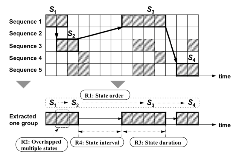
This section presents discussions of the requirements for model description using time-series data: representative data of sequential data. For this purpose, we assume a situation in which multiple different sequences are generated independently from five sensors as shown in Figure 1. Here, an observed event of which value of the sensor exceeds a predefined threshold is recognized as a ‘state’ represented in a block. The continuous period of each event is represented by the block length. Because events are not successively observed, a no-observation period exists between two successive states in certain periods. The length of such a no observation period is represented as the distance between two blocks. In this example, we also assume that a set of four black blocks, {$S_{1}$, $S_{2}$, $S_{3}$, $S_{4}$}, expresses an extracted multiple states that forms one particular group.

Now we extract the requirements for model description. First, addressing this formation of four blocks, it is readily apparent that these states are observed in a prescribed order. Therefore, it is apparent that the order of multiple states should be described in a model (R1). Second, multiple states are visible in a partially overlapped manner, as shown by $S_{1}$ and $S_{2}$. In other words, multiple states can occur simultaneously at a certain period. Therefore, the model must support the representation capability to describe multiple states occurring at the same time (R2). Third, because the time lengths of respective states mutually differ, the state duration must be expressed in a model (R3). Finally, for the case in which each state occurs intermittently, a no observation period between one state and another state that is not involved in the group of sequence might exist between two states. Furthermore, the length of this no observation period shall be variable. Therefore, the state interval between two states in a model must be described (R4). In summary, the sequential data model is required to describe these requirements. This report defines these respective requirements as follows.

1. R1: State order

2. R2: Staying multiple states in a certain period

3. R3: State duration

4. R4: State interval

Among these items, R2 differs from other items because R1, R3, and R4 are required even for a single sequence, whereas R2 is the requirement for multiple sequences. Therefore, this study specifically examines requirements R1, R3, and R4. The examination of R2 shall be left for advanced studies to be undertaken as future work.

3.2 Requirement Verification for Extended HMM Models

Table 1: Requirement satisfactions in HMM, HMM variants, and our proposals.

	Requirements
Model	Time length	Time Interval
	in a state (R3)	between states (R4)
HMM (baseline) [36]
HMM-selftrans [17]	✓
FO-HMM [19]
IO-HMM [18]
EDM [20, 21] and HSMM [8, 24]	✓
IS-HSMM and ILP-HSMM (proposal)	✓	✓

This section presents investigation of whether HMM and the extended variants of HMM satisfy those requirements. Table 1 presents a comparison among the existing HMM models from the viewpoints of the model requirements described above. Because the baseline HMM model describes the order of the states (R1), all the extended HMM models inherit this capability. FO-HMM is specialized for treating the ambiguity of observation symbols. It does not contribute to our model requirement. IO-HMM is a hybrid model of generative and discriminative models to treat the estimation probability commonly used for input sequence and observations. Therefore, it does not satisfy the remaining requirements. HSMM models the time length to remain in a single state [8]. Its variants including HMM-selftrans and EDM [20, 21, 22, 23] satisfy the same requirements: state order (R1) and state duration (R3).

As a result of investigation of the requirement satisfaction, it is apparent that no existing HMM model accommodates both the state duration and the state interval together. Nevertheless, we conclude that HSMM is the best baseline model to be extended towards our new target model because only HSMM handles state duration.

Moreover, some extended models of HSMM have been proposed. Baratchi et al. and Yu et al. proposed extended models of HSMM that can treat missing data. Their proposal can model the sequential data even if they include missing intervals [34, 35]. These studies are motivated to complement the missing data so that the ‘interval of missing’ might have variable status in all sequences. It is useful for modeling even if it has missing data and interpolating the missing data. However, in the situation we lead from the sequential data analysis described in this section, the interval is not ‘missing’. The status of the interval is only the interval which includes other status that is unrelated to the sequence. Therefore the target for modeling differs from our target. It is necessary to model the interval which is not missing. Therefore, the next section provides a detailed explanation of HSMM.

4 Hidden Semi-Markov Model (HSMM)

HMM has been studied as a powerful model for speech recognition. The model parameters of HMM consist of the initial state probability, the transition probability between states and the emission probability of observation elements from each state. The model training phase calculates the optimum values of the model parameters. The recognition phase calculates the probabilities that generates an observed sequence for each model, and then selects the highest probability model as a recognition result.

The distinguishing feature of HMM is to model the transition probability of every pair of two states. However, the time length to stay in each state cannot be modeled by HMM, which is fundamentally necessary for modeling in some useful applications such as online handwriting recognition. HSMM, which has been proposed to support this time length, has long been studied for some specific applications such as speech recognition and online handwriting recognition. This section, after providing basic notation, presents details of the algorithms of the model training and recognition in HSMM.

(a) Model structure of HMM. The state node of HMM emits an observation symbol.

(b) Model structure of HSMM. The super state node of HSMM emits observation sequence in a certain duration.

Figure 2: Model structure comparison between HMM and HSMM.

4.1 Notations

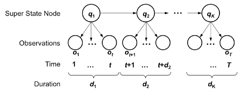
The HSMM structure is shown in Figure 2 compared with that of HMM. Hereinafter, we assume that each unit time at time $t$ has one corresponding observation $o_{t}$. The observation sequence from time $t={t_{1}}$ to $t={t_{2}}$ is denoted as $\mbox{\boldmath$o$}_{t_{1}:t_{2}}=o_{t_{1}},...,o_{t_{2}}$. A set of output symbols is expressed as $Y=\{y_{1},y_{2},\cdots,y_{N}\}$, where $N$ is the number of symbols, and $o_{t}\in Y$. A set of hidden states is $S=\{1,\cdots,M\}$, where $M$ is the number of hidden states, and the hidden state sequence from time $t=1$ to $t=T$ is expressed as $S_{1:T}=S_{1},...,S_{T}$, where $S_{t}$ represents a state at time $t$. Whereas HMM allows each state node to emit an observation symbol, HSMM has super-state node instead and each super state node can emit multiple observation symbols, i.e., observation sequence. Here the hidden state sequence is represented as $Q=q_{1},\cdots,q_{k},\cdots,q_{K}$, where $K$ is the number of states in a sequence. Also, $K=T$ in HMM, $K\leq T$ in HSMM. The $k$-th hidden state in the sequence is assigned to state $i$ as $q_{k}=i\in S$ in both HMM and HSMM.

The parameters incorporated in the HMM model are ${\mathrm{\Lambda}}=\{\mbox{\bf A},\mbox{\bf B},\mbox{\boldmath$\pi$}\}$, where $\mbox{\bf A}\in\mathbb{R}^{M\times M}$ is the matrix representing the transition probabilities between states, $\mbox{\bf B}\in\mathbb{R}^{M\times N}$ is the matrix for the emission probability from each state, and $\mbox{\boldmath$\pi$}\in\mathbb{R}^{M}$ represents the initial probability of each state. The transition probability from state $i$ to state $j$ is denoted as $\mbox{\bf A}(i,j)=a_{ij}$ where $i,j\in S$. Similarly, the emission probability of symbol $y_{n}$ from state $j$ is represented as $b_{j}(y_{n})$ and B$(j,n)=b_{j}(y_{n})$, where $j\in S$ and $y_{n}\in Y$. The initial probability that state $i$ occurs is denoted as $\pi_{i}$.

However, HSMM handles the same set of parameters $\mathrm{\Lambda}=\{\mbox{\bf A},\mbox{\bf B},\mbox{\boldmath$\pi$}\}$, but the elements of each parameter differ from those of HMM to describe the duration of states. The set of duration times is denoted as $D$; the duration of state $i$ is represented as $d_{i}\in D$. Considering this new parameter, the transition probability from state $i$ to state $j$ is represented as $a_{(i,d_{i})(j,d_{j})}$ instead of $a_{i,j}$. The emission probability is represented as $b_{j,d_{j}}(\mbox{\boldmath$o$}_{t+1:t+d_{j}})$ instead of $b_{j}(o_{t})$. Parameter $\mathrm{\Lambda}$ is updated by the recursive calculation for inference. The latest calculation result for update is represented as $\hat{\mathrm{\Lambda}}$. The overall algorithm is summarized in Algorithm 1.

Algorithm 1 Algorithm for training and recognition in HSMM.

0:  InputTraining sequences: $\mbox{\boldmath$o$}_{1:{T_{r}}}^{z}=\{o_{1}^{z},\cdots,o_{T_{r}}^{z}\}$,Testing sequences: $\mbox{\boldmath$o$}_{1:{T_{t}}}^{*}=\{o_{1}^{*},\cdots,o_{T_{t}}^{*}\}$. ($Z$ is the number of training sequences.)($H$ is the number of recursive calculation.)

0:  Training phase

1:  for $z=1$ to $Z$  do

2:      Assign random values to the HSMM parameters $\mathrm{\Lambda}^{z}=\{\mbox{\bf A},\mbox{\bf B},\mbox{\bf$\pi$}\}$, and $\alpha_{t(j,d_{j})}$ and $\beta_{t(j,d_{j})}$.

3:     for $h=1$ to $H$ do

4:        for $t=1$ to $T_{r}$ do

5:            Calculate $\alpha_{t(j,d_{j})}$ and $\beta_{t(j,d_{j})}$ using (1) and (2).

6:            Update parameters $\mathrm{\Lambda}^{z}$ using (3) and (4).

7:        end for

8:         Calculate $\theta_{h}$ using (8).

9:        if $\theta_{h}-\theta_{h-1}<\epsilon$  then

10:            break

11:        end if

12:     end for

13:  end for

13:  Recognition phase

14:  for $z=1$ to $Z$ do

15:     for $t=1$ to $T_{t}$ do

16:         Prepare $\mathrm{\Lambda}^{z}$ from the results obtained in the training phase.

17:         Calculate $\alpha_{t}(j,d_{j})$ using (9).

18:     end for

19:      Calculate $P(o_{1:T_{t}}|\mathrm{\Lambda}^{z})$ using $\alpha_{t}(j,d_{j})$.

20:  end for

21:   Select the model $z^{*}$ that has the maximum value for $P(o_{1:T_{t}}^{*}|\mathrm{\Lambda}^{z})$.

22:   Return Model $z^{*}$ and its probability $P(\mbox{\boldmath$o$}_{1:T_{t}}^{*}|\mathrm{\Lambda}^{z^{*}})$.

4.2 Model Training (Inference)

This section presents a description of how to train the model of HSMM using training sequences, i.e., how to estimate the set of parameters $\mathrm{\Lambda}=\{\mbox{\bf A},\mbox{\bf B},\mbox{\boldmath$\pi$}\}$ including the duration in each state. HSMM is trained using Baum-Welch algorithm [15] in the same way as HMM, where a recursive forward-backward algorithm is used. The forward-backward algorithm is an inference algorithm used for HMM. An extended algorithm special for HSMM is also proposed [37].

The concrete algorithm for HSMM is the following: computing forward probabilities starts from $t=1$ to $t=T$, with computed backward probabilities from $t=T$ to $t=1$. This two-way calculation repeats until the likelihood converges. More concretely, the forward step calculates the following forward variable $\alpha_{t}(j,d_{j})$ of state $j$ with $d_{j}$ at $t$ as

$$\alpha_{t}(j,d_{j}) = \sum_{i\in\{S\}\setminus\{j\}}\sum_{d_{i}\in D}\alpha_{t-{d_{j}}}(i,d_{i})a_{(i,d_{i})(j,d_{j})}b_{j,d_{j}}(\mbox{\boldmath$o$}_{t-d_{j}+1:t}).$$ (1)

The backward step calculates the following backward variable $\beta_{t}(j,d_{j})$ as

$$\beta_{t}(j,d_{j}) = \sum_{i\in\{S\}\setminus\{j\}}\sum_{d_{i}\in D}a_{(j,d_{j})(i,d_{i})}b_{i,d_{i}}(\mbox{\boldmath$o$}_{t+1:t+d_{i}})\beta_{t+d_{i}}(i,d_{i}).$$ (2)

The calculation step for estimating the model parameters are presented below.
Step 1 Initialization

Give an initial set of parameters $\mathrm{\Lambda}$ of the model at random.
Step 2 Recursive calculation

Calculate the set of parameters $\hat{\mathrm{\Lambda}}$ that maximizes the variables of the forward-backward algorithm using the initialized parameter $\mathrm{\Lambda}$. Denoting the updated state transition probability $a$ and the updated emission probability $b$ as $a^{\prime}$ and $b^{\prime}$, respectively, $a^{\prime}_{(i,d_{i})(j,d_{j})}$ and $b^{\prime}_{j,d_{j}}(\mbox{\boldmath$o$}_{t+1:t+d_{j}})$ are updated using the previous values of $a_{(i,d_{i})(j,d_{j})}$ and $b_{j,d_{j}}(\mbox{\boldmath$o$}_{t+1:t+d_{j}})$. More specifically, the state transition probability from state $i$ with $d_{i}$ to state $j$ with $d_{j}$ is defined as

$$a_{(i,d_{i})(j,d_{j})} := P(S_{t+1:t+d_{j}}=j|S_{t-d_{i}+1:t}=i).$$

Analogous to the state transition probability, the emission probability of $\mbox{\boldmath$o$}_{t+1:t+d_{j}}$ from state $j$ with $d_{j}$ is defined as

$$b_{j,d_{j}}(\mbox{\boldmath$o$}_{t+1:t+d_{j}}) := P(\mbox{\boldmath$o$}_{t+1:t+d_{j}}|S_{t+1:t+d_{j}}=j).$$

Then, these probability updates are calculated as (3) and (4) using the variables of (1) and (2) as

$$a^{\prime}_{(i,d_{i})(j,d_{j})} = {\frac{\sum_{t=1}^{{T}}\alpha_{t}(i,d_{i})a_{(i,d_{i})(j,d_{j})}{b_{i,d_{i}}(\mbox{\boldmath$o$}_{t-d_{i}+1:t})}\beta_{t+{d_{j}}}(j,d_{j})}{\sum_{t=1}^{{T}}\alpha_{t}(i,d_{i})\beta_{t}(i,d_{i})}}.$$ (3)

$$b^{\prime}_{j,d_{j}}(\mbox{\boldmath$o$}_{t+1:t+d_{j}}) = {\frac{\sum_{t=1}^{T}\delta(o_{t},y_{n})\alpha_{t}(j,d_{j})\beta_{t}(j,d_{j})}{\sum_{t=1}^{T}\alpha_{t}(j,d_{j})\beta_{t}(j,d_{j})}},$$ (4)

where $\delta(o_{t},y_{n})$ is defined as

$$\delta(o_{t},y_{n}) = \left\{\begin{array}[]{lll}1&&{if\ }o_{t}=y_{n}\\ 0&&otherwise.\end{array}\right.$$ (7)

Step 3 Parameter update and log-likelihood calculation

Update the set of parameters as $\mathrm{\Lambda}=\hat{\mathrm{\Lambda}}$ using the result of Step 2. Calculate the probability that outputs the observation sequence $\mbox{\boldmath$o$}_{1:T}$ from the current model, and finally calculate the log-likelihood as

$$\hat{\theta}\ \ =\ \ {\mathop{\rm arg~{}max}\limits_{\theta}}\log P(\mbox{\boldmath$o$}_{1:T}) = \log\sum_{j=1}^{M}\alpha_{T}(j,d_{j}),$$ (8)

where $\alpha_{T}(j,d_{j})$ is calculated using (1) when $t=T$ at the end of the sequence, and $\hat{\theta}$ is the updated log-likelihood probability.
Step 4 Convergence judgement

Judge whether the estimation process converges by evaluating that the amount of increase from the previous likelihood $\theta$ to the updated likelihood $\hat{\theta}$ in Step 3 is less than a predefined threshold $\epsilon$ as

$$\hat{\theta}-\theta < \epsilon.$$

If the condition above is satisfied, then the process is terminated. Otherwise Step 2 and Step 3 are iterated until the amount of increase converges.

4.3 Recognition using HSMM

For the recognition phase that finds the model that is most likely to generate a given target observation sequence, the probability of generating an observation sequence plays a fundamentally important role. For this purpose, we first assume that a label is assigned appropriately into each group of sequence in advance. The recognition step is defined to seek the most suitable label for a given group of sequence by calculating the label of the model that has the maximum probability as a recognition result. The probability of generating the target observation sequence is calculated using the forward algorithm used in HMM. For each model, it recursively calculates the forward variable and the probability for each state using $P(\mbox{\boldmath$o$}_{1:T})=\sum{{}_{i=1}^{M}}\alpha_{T}(i,d_{i})$, which is the marginal probability distribution, where

$$\alpha_{t}(j,d_{j}) = \left[{\sum_{i=1}^{M}\alpha_{t-{d_{j}}}(i,d_{i})a_{(i,d_{i})(j,d_{j})}}\right]b_{{j,d_{j}}}(\mbox{\boldmath$o$}_{t-d_{{j}}+1:t}).$$ (9)

Here, we designate the probability explicitly as $P(\mbox{\boldmath$o$}_{1:T}^{*}|\mathrm{\Lambda}^{z})$ using the parameter set of model $z$, i.e., $\mathrm{\Lambda}^{z}$, where $z\in\{1,2,\cdots,Z\}$ and $Z$ are the total number of models. Finally, the label that has the maximum $P(\mbox{\boldmath$o$}_{1:T})$ for the observation sequence is selected as the recognition result. Consequently, the model $z^{*}$ that has the maximum probability $P(\mbox{\boldmath$o$}_{1:T}^{*}|\mathrm{\Lambda}^{z})$ among all $Z$ models is selected as a result of the recognition.

5 State Interval Modeling in HSMM

This section presents investigation of how to model a state interval in a model using HSMM. Before explaining the details, we describe how to represent state interval in a sequence. The baseline HSMM model ignores the period when no event is observed because the occurrence of events and the order of the events are necessary for sequential data modeling. However, we also consider this period the no-observation period because it is also necessary to model sequential data as described in Section 3.1. Therefore, we regard this period as the state interval in this paper, and assign a new symbol “interval symbol” to this period. Figure 3 portrays an example of the state interval representation, where “a” and “b” are symbols that are actually observed in the original sequence, and “i” is the interval symbol used to fill the state interval. Section 5.1 examines the approaches for modeling state interval using HSMM. The issues that arise because of the filled sequence with state interval are addressed in Section 5.2.

Figure 3: Representation of state interval in a sequence.

5.1 Two Approaches for State Interval Modeling

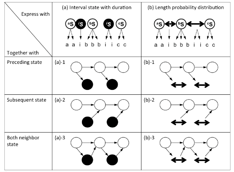
To treat state interval with HSMM, two approaches can be considered as shown in Figure 4. One represents the state interval as a new state node, which is represented as a black node as Figure 4(a). Each state of HSMM can represent its duration for staying in a single state. Therefore, this new approach describes the length of the state interval by introducing the new state node that explicitly indicates the state interval. However, the other approach represents the state interval as a new probabilistic parameter as shown in Figure 4(b).

For both approaches, three variations to model the state interval can be considered. The first approach models the state interval with the preceding state ((a)-1, (b)-1); the second models it with the subsequent state ((a)-2, (b)-2). The last variation models the length of the interval with both preceding and subsequent states ((a)-3, (b)-3). Compared among three variations, the first two models have connection with only one state whereas the last one ((a)-3, (b)-3) has connections with two states. Therefore, (a)-3 and (b)-3 can model the sequential data more precisely.

Figure 4: Two approaches for the state interval. The circle represents a state and $\rightarrow$ represents the transition from the left state to the right state. Circle filled with black and $\leftrightarrow$ represent the state interval.

5.2 Problems of State Interval Modeling

Before describing the proposed models, the technical issues for the state interval modeling in each approach in the preceding subsection are explained. The structure of the first approach is presented in Figure 5, where the interval state node is presented as a black node ${}^{i}S$. Although this approach handles the state interval in a simple way, it causes large bias in the transition probability when there are many groups of terms of observed interval symbols in a sequence as shown in Figure 6. Figure 6(a) presents an example sequence for the explanation. Each sequence shows the original observation sequence and the state sequence. Figure 6(b) presents an example sequence filled with state interval nodes of interval symbol i. The tables represented at the right of the figure show the transition frequency from a state to another state calculated using the original/complemented sequence. Whereas the states described in a vertical line in the table show the “from” states, the states in a horizontal line show the “to” state. The table in (a) shows the transition frequency calculated using the original state sequence. The table in (b) shows the transition frequency calculated using the converted state sequence filled with interval states. Accordingly, the results reveal that the transition frequency in the cells in the bold-framed area except for gray painted cells falls dramatically to lower level, i.e., nearly zero. This means that, the introduction of the interval state node causes a deviation to the original transition probability. The resultant new model fails to represent the transition sequence properly.

Figure 5: HSMM with an interval state.

(a) Original sequence and transition frequency.

(b) Filled sequence and transition frequency.

Figure 6: Problem of sequence with a state interval.

For the second approach in the preceding subsection, the manner of representing a state interval with the new probabilistic parameter “interval length probability” must be defined. Considering the application data, the model is expected to be found such that sequential data have a similar sequential pattern with similar state duration and similar state interval. Therefore, it is necessary to model the state duration and the state interval with representation of the similarity of its time length. Therefore, the second approach defines how to represent the new parameter for state duration and how to model the parameters with the original HSMM in a probabilistic manner.

Addressing these problems, finally, we propose two extended models in the following sections: an interval state hidden semi-Markov model (IS-HSMM) as the first approach, and an interval length probability hidden semi-Markov model (ILP-HSMM) for the second approach.

6 Interval State Hidden Semi-Markov Model (IS-HSMM)

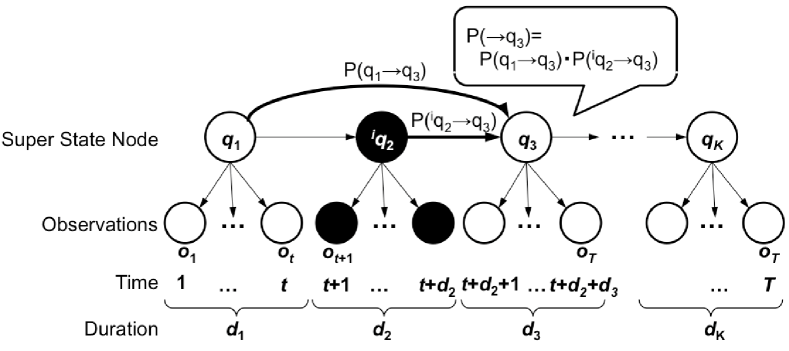
Actually, HSMM handles the state interval in a simple way because the interval symbol is replaced with the new interval state node as described in Section 5. However, we face the difficulty of the degradation of the accuracy of the transition probability in cases where state intervals appear frequently in the same sequence. To resolve this difficulty, we propose an extended model, IS-HSMM, to preserve the transition probability of the original sequence. Figure 7 presents a conceptual structure of IS-HSMM. For easy-to-understand explanation, we select the first three states shown in Figure 7 as an example when $q_{1}$ and $q_{{3}}$ are original hidden states and ${{}^{i}}q_{{2}}$ is the interval state node. Whereas the original HSMM infers the transition probability in the order of $q_{1}$, ${}^{i}q_{2}$, and $q_{3}$, the proposed IS-HSMM infers the transition probability as $q_{3}$ using two transition probabilities not only from ${}^{i}q_{2}$ to $q_{3}$, but also from the previous $q_{1}$ to $q_{3}$ to preserve the transition of the original sequence. This is a noteworthy feature of IS-HSMM. This section explains how to train and how to recognize the model as follows.

Figure 7: Conceptual structure of IS-HSMM with an interval state node using two transition probabilities.

6.1 Model Training in IS-HSMM

The difference against the baseline HSMM model appears in the calculation of the forward variables and backward variables in the recursive calculation step. The state transition probability from state $i$ to state $j$, where the interval state ${}^{i}s$ is inserted between state $i$ and state $j$, is defined as

$$a_{(i,d_{i})(^{i}s,^{i}d)(j,d_{j})} := P(S_{t+{{}^{i}d+}1:t+{{}^{i}d+}d_{j}}=j|S_{t+1:t+^{i}d}=^{i}s,~{}S_{t-d_{i}+1:t}=i)$$

$$:= P(S_{t+1:t+d_{j}}=j|S_{t-^{i}d+1:t}=^{i}s,~{}S_{t-d_{i}-d_{i}+1:t-^{i}d}=i)$$

where the duration of interval state ${}^{i}s$ is denoted as ${}^{i}d$($>0$). The respective durations of state $i$ and $j$ are $d_{i}$ and $d_{j}$. The transition $a_{(i,d_{i})(^{i}s,^{i}d)(j,d_{j})}$ is calculated with the transition from ${}^{i}s$ and the preceding state $s_{i}$ only when calculating after ${}^{i}s$. Therefore, the forward variable, where the current state is $j$ and the preceding state is ${}^{i}s$, is calculated using the further preceding state $i$ based on the second-order HMM [38] as

$$\alpha_{t}((^{i}s,^{i}d),(j,d_{j})) = \sum_{i\in\{S\}\setminus\{j,^{i}s\}}\sum_{d_{i}\in D}\alpha_{t-^{i}d}((i,d_{i}),(^{i}s,^{i}d))\cdot a_{(i,d_{i})(^{i}s,^{i}d)(j,d_{j})}b_{j,d_{j}}(o_{t-^{i}d+1:t}),$$ (10)

where $a_{(i,d_{i})(^{i}s,^{i}d)(j,d_{j})}$ is updated the following equation.

$$a^{\prime}_{(i,d_{i})(^{i}s,^{i}d)(j,d_{j})} = \sum_{t=1}^{T-d_{j}-^{i}d}\alpha_{t+^{i}d}((i,d_{i}),(^{i}s,^{i}d))a_{(i,d_{i})(^{i}s,^{i}d)(j,d_{j})}\cdot b_{j,d_{j}}(o_{t+^{i}d+d_{j}})\beta_{t+^{i}d+d_{j}}(j,d_{j})$$

$$\big{/}\sum_{t=1}^{T-d_{j}-^{i}d}\sum_{j\in\{S\}\setminus\{i,^{i}s\}}\alpha_{t+^{i}d}((i,d_{i}),(^{i}s,^{i}d))a_{(i,d_{i})(^{i}s,^{i}d)(j,d_{j})}\cdot b_{j,d_{j}}(o_{t+^{i}d+d_{j}})\beta_{t+^{i}d+d_{j}}(j,d_{j}).$$

Then, the backward variable where the preceding state is ${}^{i}s$ is calculated as general first-order transition probabilities expressed as

$$\beta_{t}(j,d_{j}) = \sum_{i\in\{S\}\setminus\{j\}}\sum_{{}^{i}d\in D}a_{(j,d_{j})(^{i}s,^{i}d)}b_{{}^{i}s,^{i}d}(\mbox{\boldmath$o$}_{t+1:t+^{i}d})\beta_{t+^{i}d}(^{i}s,^{i}d).$$ (11)

Finally, the transition probability and the emission probability are updated using (10) and (11) by calculating the state transition probability using (6.1) and assigning the forward and backward variables obtained respectively using (3) and (4).

6.2 Recognition using IS-HSMM

Although calculation of the probability follows the original HSMM when the preceding state is not the interval state node, it differs when the preceding state is the interval state node. The probability of the observation sequence when the preceding state is the interval state node is calculated as $P(\mbox{\boldmath$o$}_{1:T})=\sum_{i=1}^{M}\alpha_{T}(i,d_{i})$, where (9) and the follows:

$$\alpha_{t}(j,d_{j})=\left[\sum_{i=1}^{{M}}\alpha_{t-{d_{j}-^{i}d}}(i,d_{i})a_{(i,d_{i})(^{i}s,^{i}d)}{\cdot a_{(^{i}s,^{i}d)(j,d_{j})}}\right]b_{{}^{i}s,^{i}d}(\mbox{\boldmath$o$}_{t-^{i}d-d_{j}+1:t-d_{j}})\cdot b_{j,d_{j}}(\mbox{\boldmath$o$}_{t-d_{j}+1:t}),\ \$$ (12)

where the preceding state is ${}^{i}s$. The overall algorithm is presented in Algorithm 2.

Algorithm 2 Algorithm for training and recognition in IS-HSMM.

0:  InputTraining sequences: $\mbox{\boldmath$o$}_{1:T_{r}}^{z}=\{o_{1}^{z},\cdots,o_{T_{r}}^{z}\}$, Testing sequences: $\mbox{\boldmath$o$}_{1:T_{t}}^{*}=\{o_{1}^{*},\cdots,o_{T_{t}}^{*}\}$. ($Z$ is the number of training sequences.)($H$ is the number of recursive calculation.)

0:  Training phase

1:  for $z=1$ to $Z$ do

2:      Assign random values to the HSMM parameters $\mathrm{\Lambda}=\{\mbox{\bf A},\mbox{\bf B},\mbox{\bf$\pi$}\}$, and $\alpha_{t(j,d_{j})}$ and $\beta_{t(j,d_{j})}$.

3:     for $h=1$ to $H$ do

4:        for $t=1$ to $T_{r}$ do

5:           if $o_{t-1}$ is interval symbol then

6:               Calculate $\alpha_{t(j,d_{j})}$ and $\beta_{t(j,d_{j})}$ with joint probability from $i$ and ${}^{i}s$ using (10) and (11).

7:           else

8:               Calculate $\alpha_{t(j,d)}$ and $\beta_{t(j,d_{j})}$ with preceding state $i$ using (1) and (2).

9:           end if

10:            Update parameters $\mathrm{\Lambda}$.

11:        end for

12:         Calculate $\theta_{h}$ using (8) with (10).

13:        if $\theta_{h}-\theta_{h-1}<\epsilon$ then

14:           break

15:        end if

16:     end for

17:  end for

17:  Testing phase

18:  for $z=1$ to $Z$ do

19:     for $t=1$ to $T_{t}$ do

20:        if $o_{t-1}$ is the interval symbol then

21:            $\mathrm{\Lambda}^{z}$ $\leftarrow$ parameter $\mathrm{\Lambda}$ of model $z$ with joint probability from $j$ and ${}^{i}s$.

22:        else

23:            $\mathrm{\Lambda}^{z}$ $\leftarrow$ parameter $\mathrm{\Lambda}$ of model $z$ with preceding state $j$.

24:        end if

25:         Calculate $\alpha_{t}(j,d_{j})$ using (9) with (12).

26:     end for

27:      Calculate $P(o_{1:T_{t}}|\mathrm{\Lambda}^{z})$ using $\alpha_{t}(j,d_{j})$.

28:  end for

29:   Select the model $z^{*}$ that has the maximum value for $P(\mbox{\boldmath$o$}_{1:T_{t}}^{*}|\mathrm{\Lambda}^{z})$.

30:   Return Model $z^{*}$ and its probability $P(\mbox{\boldmath$o$}_{1:T_{t}}^{*}|\mathrm{\Lambda}^{z^{*}})$.

7 Interval Length Probability HSMM (ILP-HSMM)

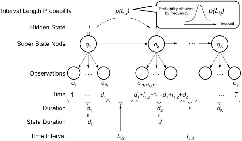
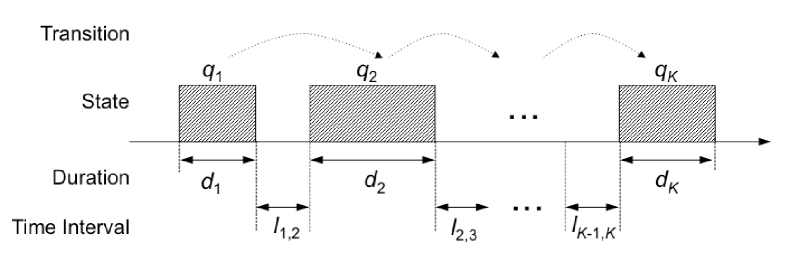
This section presents ILP-HSMM, which newly introduces interval length probability to the transition probability to handle the state interval between two states. It is noteworthy that the interval length probability corresponds to the probability density distribution of interval length of two states, to be technically precise. The distinct difference between HSMM and ILP-HSMM is that, whereas state $j$ starts immediately after the end time of state $i$ in the original HSMM, state $j$ starts after a length of time, $L_{i,j}$, passes since the end time of state $i$ in ILP-HSMM. The conceptual model structure of ILP-HSMM is presented in Figure 8. Although the ILP-HSMM structure is similar to that of HSMM presented in Figure 2, the interval length probability is newly added to HSMM as shown in Figure 8, where $L_{i,j}$ represents the time difference between the end time of state $i$ and the beginning time of state $j$. It is noteworthy that the total time length of the observation sequence $T$ varies because of its dependency on the length of state duration and interval, leading to $T=\Sigma^{K}_{k=1}(d_{k}+l_{k-1,k})$, where $l_{k-1,k}$ is the time difference between the end of $q_{k-1}$ and the beginning of $q_{k}$. The subsequence section presents a description of how to model and how to recognize given datasets using ILP-HSMM.

Figure 8: Conceptual structure of ILP-HSMM using state interval probability.

7.1 Model Training (Inference) in ILP-HSMM

Figure 9 presents example data and representations used hereinafter for explanation. The slash line patterned blocks represent the data sequence of the training dataset. First, the probability density distribution of the interval length of $L_{i,j}$ is expressed by the Gaussian distribution $p(L_{i,j})$ as

$$p(L_{i,j})~{}=~{}\frac{1}{\sqrt{2\pi\sigma^{2}}}e^{-{\frac{(L_{i,j}-\mu)^{2}}{2\sigma^{2}}}},$$ (13)

where $\sigma$ and $\mu$ respectively present the variance and the mean of $L_{i,j}$. It is noteworthy that the Gaussian distribution is adopted as the probability density distribution, for simplicity. However, other distributions and functions were adopted for ILP-HSMM without changing any other parameter. Accordingly, the set of parameters used in ILP-HSMM is defined as

$$\mathrm{\Lambda}:=\{\mbox{\bf A},\mbox{\bf B},\mbox{\boldmath$\pi$},\mbox{\bf L}\},$$

where the elements of the parameter $\mathrm{\Lambda}$ take on $\mbox{\bf A}(i,j)=a_{(i,d_{i})(j,d_{j})}$, $\mbox{\bf B}(j,n)=b_{(j,d_{j})}(\mbox{\boldmath$o$}_{1:d_{j}})$, and $\mbox{\boldmath$\pi$}(i)=\pi_{j,d_{j}}$, where $d_{i}\in D$ represents the duration of state $i$ described in Section 4.1. Furthermore, $\mbox{\bf L}\in\mathbb{R}^{M\times M}$ is the matrix that consists of the interval length probabilities, i.e., the probability density distributions of the length of state interval, where $\mbox{\bf L}(i,j)=p(L_{i,j})$. The transition and emission probabilities are defined as the same as those in HSMM. The difference between HSMM and ILP-HSMM is to consider the parameter of $p(L_{i,j})$.

The range of $L_{i,j}$ in (13) might influence either memory consumption or computational complexity to generate the model. There might be no $L_{i,j}$ value suitable for the observation values because of the range limitation of $L_{i,j}$ if $p(L_{i,j})$ is generated in a training period. However, if the parameter $p(L_{i,j})$ is generated every time an observation is fed to the algorithm, then the calculation cost can be much higher. Our motivation to introduce the interval length probability to HSMM is, as explained earlier, to find the similar part of sequential data with respect to the state interval and also to discriminate between the target part and the similar part. Therefore, even if the probability of $L_{i,j}$ is presumed to be zero around the skirts of the distribution, no critically important difficulty arises. Consequently, we introduce the boundary of the probability value $\delta_{pt}$ to ascertain the edge of the skirt of $p(L_{i,j})$. On generating the $p(L_{i,j})$, the calculation is terminated when the probability value becomes less than $\delta_{pt}$. The probability of $p(L_{i,j})$ is zero outside of the range of $\delta_{pt}$.

Figure 9: Sequential data and representations.

7.2 Recognition using ILP-HSMM

The Viterbi algorithm is used to estimate the probability of a model [23]. The pair of the model with the interval length probability and its label that is expected to be estimated are stored as candidates for estimation. The recognition label that denotes the estimated result is selected when the model has the maximum likelihood estimate by calculating it for each state in each model.

First, we calculate $p(L_{i,j})$ beforehand. If $L_{i,j}$ is out of the range, then the probability density distribution is determined as

$$p(L_{i,j}) = \min_{i,j\in S}p(L_{i,j})\times c,$$

where $c$ is $0\leq c\leq 1$. Then, the forward variable for estimating the maximum likelihood is calculated as

$$\alpha_{t}(j,d_{j}) = \left[\sum_{i=1}^{M}\alpha_{t-{d_{j}}}(i,d_{i})a_{(i,d_{i})(j,d_{j})}\cdot p(L_{i,j})\right]b_{j,d_{j}}(\mbox{\boldmath$o$}_{t-d_{j}+1:t}).$$ (14)

The interval length probability is calculated simultaneously with calculation of the parameter of the likelihood using the transition probability recursively.

The difference between HSMM and ILP-HSMM is the capability of handling the length of the state interval between states as explained earlier. The interval length probability in ILP-HSMM can be integrated by introducing each interval into two pair of states to calculate the likelihood. This calculation might produce an additional calculation cost. Therefore, it is necessary to evaluate the calculation cost. In addition, the emission probability $b_{j,d_{j}}({\bf o}_{1:d_{j}})$ can be parametric or non-parametric. In this proposal, the relation between the state duration and the state interval is not represented in a model. For this reason, $b_{j,d_{j}}({\bf o}_{1:d_{j}})$ is handled as non-parametric, discrete, and independent of the duration. Then, $p(L_{i,j})$ is also discrete and independent of the duration and the transition probability.

Algorithm 3 Algorithm for training and recognition in ILP-HSMM.

0:  InputTraining sequences: $\mbox{\boldmath$o$}_{1:T_{r}}^{z}=\{o_{1}^{z},\cdots,o_{T_{r}}^{z}\}$,Testing sequences: $\mbox{\boldmath$o$}_{1:T_{t}}^{*}=\{o_{1}^{*},\cdots,o_{T_{t}}^{*}\}$. ($Z$ is the number of training sequences.)($H$ is the number of recursive calculation.)

0:  Training phase

1:  for $z=1$ to $Z$ do

2:      Assign random values to the HSMM parameters $\mathrm{\Lambda}=\{\mbox{\bf A},\mbox{\bf B},\mbox{\bf$\pi$},\mbox{\bf L}\}$, and $\alpha_{t(j,d_{j})}$ and $\beta_{t(j,d_{j})}$. Initialize $p(L_{i,j})$ as $L_{i,j}=1$.

3:     for $h=1$ to $H$ do

4:        for $t=1$ to $T_{r}$ do

5:            Calculate $\alpha_{t(j,d_{j})}$ and $\beta_{t(j,d_{j})}$ using (1) and (2).

6:            Calculate $p(L_{i,j})$ with $i$ and $j$ using (13).

7:            Update parameters $\mathrm{\Lambda}$.

8:        end for

9:         Calculate $\theta_{h}$ using (12).

10:        if $\theta_{h}-\theta_{h-1}<\epsilon$ then

11:           break

12:        end if

13:     end for

14:  end for

14:  Testing phase

15:  for $z=1$ to $Z$ do

16:     for $t=1$ to $T_{t}$ do

17:         $\mathrm{\Lambda}^{z}$ $\leftarrow$ parameter $\mathrm{\Lambda}$ of model $z$.

18:         $p(l)$ $\leftarrow$ $p(L_{i,j})$ using $\mathrm{\Lambda}^{z}$ with observed interval $l$.

19:         Calculate $\alpha_{t}(j,d_{j})$ using (9) with (14).

20:     end for

21:      Calculate $P(o_{1:T_{t}}|\mathrm{\Lambda}^{z})$ using $\alpha_{t}(j,d_{j})$.

22:  end for

23:   Select model $z^{*}$ with the maximum value for $P(\mbox{\boldmath$o$}_{1:{T_{t}}}^{*}|\mathrm{\Lambda}^{z})$.

24:   Return Model $z^{*}$ and its probability $P(\mbox{\boldmath$o$}_{1:T}^{*}|\mathrm{\Lambda}^{z^{*}})$.

8 Evaluations

This section presents a description of the performance evaluation of models. After explaining the specifications of the experimental data in Section 8.1, Section 8.2 and Section 8.3 present the experimentally obtained results of the execution time and recognition performance comparison among HSMM, IS-HSMM, and ILP-HSMM. Finally, we evaluate a reproducibility comparison between IS-HSMM and ILP-HSMM in terms of the modeling performance in Section 8.4.

8.1 Experimental Data

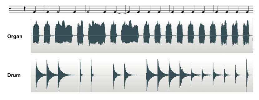
Addressing that the sequential data contain the state duration and the state interval, we use music sound data played by instruments of different kinds. When the same music is played by the different instruments, even if the music rhythm is the same, the length of each sound for the same note differs. For example, the sound power spectrum played by an organ and a drum for the same music sound data is shown in Figure 10. The horizontal axis shows the time. The vertical axis shows the sound power, i.e., sound volume. Whereas the power of each note played by the organ is almost identical during the sound resonation, the one played by the drum decreases rapidly after tapping. We generate the observation sequence from the music sound data. The generation step is described below using the features of sound continuous time.
Step 1

Set thresholds $b_{1}$ and $b_{2}$ to classify the observation symbols into three types by the level of the volume. $b_{1}$ is a threshold for determining whether the sound is “on” or “off”, and $b_{2}$ is the one for classifying the power of the sound as “high” or “low”. $(b_{2}\geq b_{1})$
Step 2

For the sound power $v$ of each time, the observation sequence is generated as follows.

If $v\geq b_{2}$, then the observation symbol is “high”.

If $b_{2}>v\geq b_{1}$, then the observation symbol is “low”.
An example of observation sequence generated by the procedure described above is shown in Figure 11. The black cell represents the “high” symbol. The gray cell represents a “low” symbol. The white-painted cells represent the “interval.” To denote the segment of a sequence, we add “start” and “end” symbols to each edge of the sequence. These symbols are useful for modeling the transition from the initial state from sequences precisely. The dataset consists of 27 segmented data, which are divided into bars of the music sequence. A label is assigned for each 27 segmented data. Therefore the number of labels is also 27. The kinds of the instruments are a grand piano, horn, drums, acoustic guitar, flute, and pipe organ. We use the music sound data played by the instruments of the first three kinds for training data, whereas the latter three kinds are used for recognition data. The numbers of the sequential data are 81 for both training and recognition.

Figure 10: Music sound data.

Figure 11: Example sequences generated using music sound data.

8.2 Execution Time Evaluation

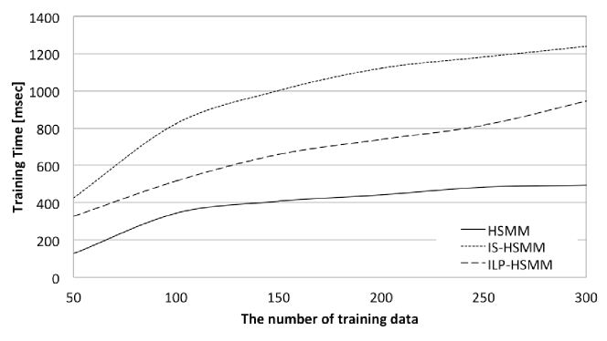
This section presents the execution time evaluation for training and recognition. For the evaluation, we generate 35 sequences, fixing $d_{min}=d_{max}=2$, $l_{min}=1$, and $l_{max}=10$, where $T$ is not fixed a priori. Using the generated data, we compare the training time and recognition time while changing the number of training data. The training time results are presented in Figure 12. The $x$-axis shows the number of training data. The $y$-axis shows the execution time for training. The upper, middle, and bottom lines respectively present the results of IS-HSMM, ILP-HSMM, and HSMM. Results show that three graphs are mostly increasing parallel, which shows that the difference between the results of HSMM and IS-HSMM, and the difference between the results of HSMM and ILP-HSMM are both of a certain degree. Therefore, the training time of IS-HSMM and ILP-HSMM requires additional time, but the amount of the additional time does not increase exponentially.

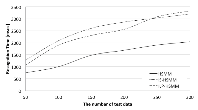
Similarly, the execution time for recognition is shown in Figure 13. The $x$-axis shows the number of test data. The $y$-axis shows the execution time for recognition. The upper, middle, and bottom lines respectively present the results of IS-HSMM, ILP-HSMM, and HSMM. Results show that the amount of the additional time for recognition does not increase exponentially to the same degree as training. Stated differently, both the evaluation results of training time and recognition time reveal that it causes no severe difficulty for the execution times.

Figure 12: Execution time for training.

Figure 13: Execution time for recognition.

8.3 Recognition Performance Evaluation

This section presents the evaluation results of recognition performance comparing IS-HSMM and ILP-HSMM with HSMM. The evaluation metric is the recognition accuracy based on the f-measure calculated using
${{\it f}-measure~{}=~{}(2\cdot{\rm recall}\cdot{\rm precision})/({\rm recall}+{\rm precision})}$, where ${\rm precision}=TP/PP$, and ${\rm recall}=TP/AP$. Here, the Predicted Positive ($PP$) is the number of models with likelihood calculated using (9) is maximum in all models. True Positive ($TP$) is the number of collected models in $PP$. Actually Positive ($AP$) is the number of labeled models.

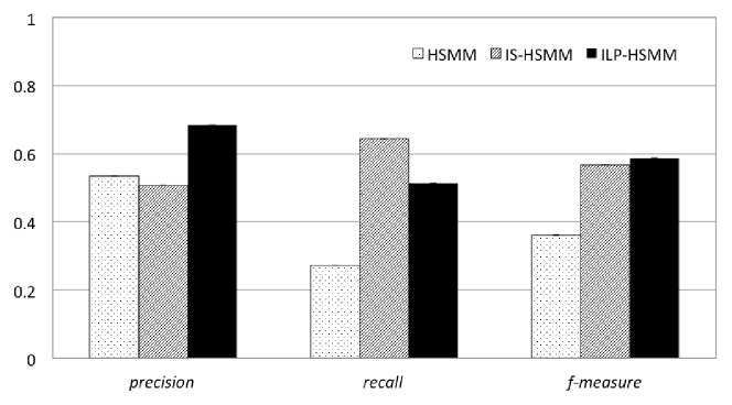
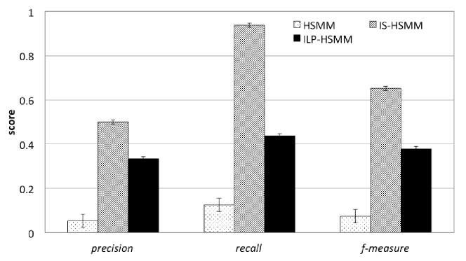
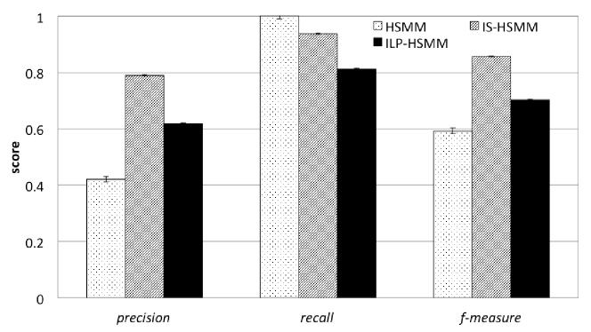
Results are presented in Figure 14 and Figure 15. The $x$-axis shows Precision, Recall, and f-measure. The $y$-axis shows the score. The left, middle, and right bars respectively present the results of HSMM, IS-HSMM, and ILP-HSMM. Figure 14 shows the results obtained when the number of states is five, and Figure 15 presents the results obtained when the number of states is ten. Both results are the average scores of five repetitions. The results show that both the proposed models IS-HSMM and ILP-HSMM have higher recognition performance than HSMM. By comparing the results of IS-HSMM and ILP-HSMM, the scores of f-measure are similar, but the scores of recall and precision differ. IS-HSMM has a higher score for recall, but it has lower score for precision than ILP-HSMM. The next section presents detailed analysis of the performances of IS-HSMM and ILP-HSMM. Finally, comparison of the two results obtained when the numbers of states are five and ten shows that the recognition performance can be higher depending on the number of states increasing.

Figure 14: Recognition performance: the number of states is 5.

Figure 15: Recognition performance: the number of states is 10.

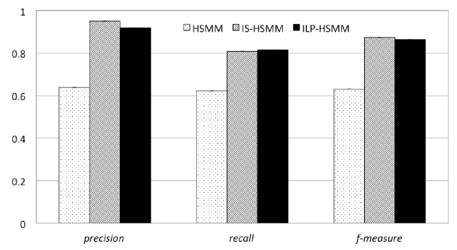
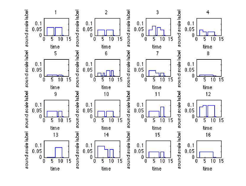
The earlier experiment includes observation symbols of only three kinds. To evaluate the performance of treating various durations and intervals with observation symbols of many kinds, we use the musical scale instead of the volume of the sound as observation symbols. Figure 16 shows the musical scale with stairs of example data. These are the some input data extracted from the evaluation data. The figure on the top of each graph signifies the label. Each value from 0.01 to 0.12 in 0.01 intervals is assigned to C, C#, D, D#, E, F, F#, G, G#, A, A#, B of the musical scale. If the volume is lower than a threshold, then the value of the sound scale label is zero. This is the interval observation in a sequence. The results of recognition performance using the data generated as described above are shown in Figure 17 and Figure 18. They present results of recognition performance evaluation when the numbers of states are 2 and 10. The scores are the average scores of five repetitions. Considering that it would be high performance when the number of states is greater than the number of observation symbols in HSMM, we assign 2 and 10 as the numbers of states in the experience to compare their performance.

Figure 16: Musical scale of example input sequences and their labels.

When the number of states is 2, the recognition performance of HSMM is extremely low, but those of IS-HSMM and ILP-HSMM are much higher than HSMM. In addition, the results of IS-HSMM are much higher than ILP-HSMM. However, when the number of states is 10, the number of states is greater than the number of the observation symbols. At this time, the entire scores of HSMM, IS-HSMM, and ILP-HSMM are higher than 0.4. For the HSMM, the recall score gives the max score in all models but the precision score represents the lowest value. Therefore, the probability for each sequence using HSMM is similar to that of each other sequence. Then, whereas the average scores of precision, recall, and f-measure are more than 0.8 in IS-HSMM, the average score is about 0.7 in ILP-HSMM. As a result, when the number of states increases, the scores of IS-HSMM are higher than those of ILP-HSMM because increasing the states contributes to treatment of the transition probability from a state to another state. Therefore, IS-HSMM is effective for treating the order of the sequence precisely because it can model the transition probability between two states as the original HMM and it can represent “interval” as one of the states.

However, regarding the input data shown in Figure 16 in detail, No. 4 input data are similar to No. 7; the No. 2 input data are similar to No. 10. It is difficult to distinguish the small time difference between two sequences with both IS-HSMM and ILP-HSMM even if the number of states increases. This difficulty might cause a decline of recognition performance.

Moreover, ILP-HSMM treats the state interval using the new additional parameter between two stationary states. If the state interval is mostly similar between static two states, then ILP-HSMM can model the length of the interval precisely, but it is difficult to model a sequence including various lengths of durations and intervals. Therefore, to treat sequential data of various kinds with durations and intervals, IS-HSMM would engender higher performance than ILP-HSMM. The following section presents evaluation results of modeling performance and analysis between ILP-HSMM and IS-HSMM.

Figure 17: Recognition performance with music scale label: the number of states is 2.

Figure 18: Recognition performance with music scale label: the number of states is 10.

8.4 Reproducibility Performance Evaluations between IS-HSMM and ILP-HSMM

This section presents the evaluation results of modeling performance, particularly addressing the performance of reproducibility. We calculate the performance of reproducibility and compare both IS-HSMM and ILP-HSMM. The performance of reproducibility signifies how precisely the model generates the original sequence, which is represented as $r$. The $r$ is calculated as

$$\hskip 14.22636ptr = \frac{\sum_{t=1}^{T}(w_{t}=o_{t})}{T},$$

where $\mbox{\boldmath$o$}_{1:T}$ stands for the original sequence, $T$ represents the time length of the original sequence, and $w_{1:T}$ denotes the generated sequence using the model parameter $\theta$ which is calculated using the original sequence. To calculate the equation presented above, we give the sequence length $T$ and generate a sequence which has high likelihood using the forward algorithm with the set of parameters $\mathrm{\Lambda}$. The generated sequence is the estimated sequence. Therefore, the performance of reproducibility indicates how precisely the model, i.e., the set of parameters $\mathrm{\Lambda}$ decided by the training phase, generates the original sequence.

Figure 19: Performance of reproducibility when the number of states increases.

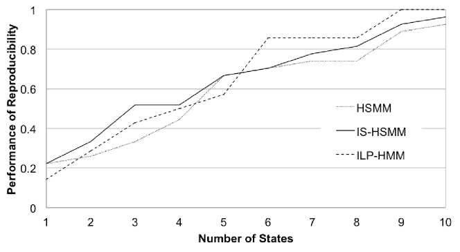
First, we evaluate the performance of reproducibility when the number of states changes. Figure 19 presents the results of evaluating reproducibility using HSMM, IS-HSMM, and ILP-HSMM. The $x$-axis shows the number of states. The $y$-axis shows the performance of reproducibility. The number of observed symbols in sequence $N$ is $N=7$.

Results show that the performance of reproducibility of all models rises as the number of states increases. The performance results of IS-HSMM and HSMM is mostly the same and IS-HSMM has a bit higher performance than that of HSMM. The results of ILP-HSMM show less performance when the states are fewer than six. They show higher performance when the number of states is greater than six i.e., the number of observed symbols. It represents that the number of states is more than the number of observed symbols; ILP-HSMM has higher performance of reproducibility than other models.

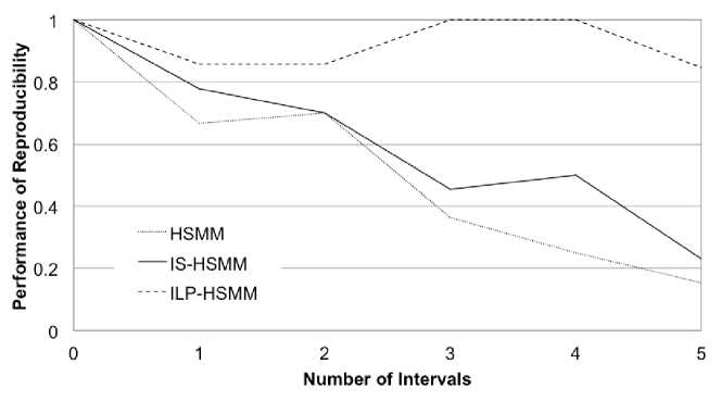
Then, we evaluate the performance of reproducibility when the number of intervals in a sequence changes. Figure 20 also shows the scores of performance of reproducibility of HSMM, IS-HSMM and ILP-HSMM. The $x$-axis shows the number of intervals in a sequence. The $y$-axis shows the score of performance of reproducibility. The number of sorts observed in a sequence is $N=6$. One of the sorts is an interval. Results show that the performance of reproducibility of both models; HSMM and IS-HSMM decrease as the number of intervals increases, but that of IS-HSMM is higher than that of HSMM. Then, the results of ILP-HSMM is the highest performance in all models. It can obtain the highest performance irrespective of the number of intervals. Therefore, IS-HSMM can model the sequence with intervals more precisely than HSMM. The ILP-HSMM can model it most precisely of all models. Comparing two results of HSMM and IS-HSMM ensures that the proposed IS-HSMM can model the sequential data more precisely than HSMM by introducing the special state, i.e., the interval state and calculating the transition probability from the state before the interval state. In addition, the performance of IS-HSMM is much higher especially when the states are few and even if many intervals exist in a sequence. Comparing the other results for IS-HSMM and ILP-HSMM ensures that the proposed ILP-HSMM can model the sequential data more precisely than other models because it represents the length of intervals directly in the model.

Figure 20: Performance of reproducibility when the number of intervals increases.

As a result of the evaluation presented above, both the proposed extension models for HSMM have higher performance than HSMM, but ILP-HSMM can model the static interval between two states. However, it is more important for modeling the general duration and interval using a model with trained multiple data which have the same label. From the perspective of modeling generalization, the recognition performance of IS-HSMM has a higher score than other models, especially where the number of sorts of the observation symbols is larger. Therefore, we conclude that IS-HSMM has higher performance for modeling the general sequential data, not only for the data which have a static length of interval, but also for data which have various interval lengths.

9 Summary and Future Work

The goal of this research was to model sequential data, including state duration and the state interval, simultaneously. We specifically examined a hidden semi-Markov model (HSMM) to treat such sequential data, and proposed two extended models to treat a state interval in a sequence: IS-HSMM and ILP-HSMM. IS-HSMM introduces a special calculation technique to treat an interval state, where if the preceding state is an interval state, it models the transition from the second preceding state to the current state simultaneously. However, ILP-HSMM uses the Gaussian distribution as a length parameter, and trains with both preceding and subsequent states. Comparisons of recognition performance and elapsed time among IS-HSMM, ILP-HSMM, and HSMM show that both of the proposed models give higher performance than HSMM although they need additional calculation costs. Comparison results between IS-HSMM and ILP-HSMM in terms of the modeling performance reveal that ILP-HSMM has higher performance than that of IS-HSMM.

As direction of future research, we intend to use our model to treat such actual sensing data which have a feature of rhythm or timing patterns. Although ILP-HSMM has higher performance in the evaluation, the concept of IS-HSMM is simpler than that of ILP-HSMM. Additionally, IS-HSMM can adopt another difficulty of analyzing sequential data, except for only treating intervals between states. In case the same state occurs frequently in a sequence, it is difficult to model the original sequence precisely without an interval. Therefore, we must evaluate the effectiveness of treating the original sequence using other application data, and finally extend the model further.

References

- [1] H Narimatsu and H Kasai. State duration and interval modeling in hidden semi-Markov model for sequential data analysis. Annals of Mathematics and Artificial Intelligence, 81(3–4):377–403, 2017.
- [2] M Esmaeili and F Gabor. Finding sequential patterns from large sequence data. International Journal of Computer Science Issues (IJSC), 7(1):43–46, 2010.
- [3] D D Lewis and W A Gale. A sequential algorithm for training text classifiers. Proc. of ACM the 17th Annual International Conference on Research and Development in Information Retrieval (ACM SIGIR), pages 3–12, 1994.
- [4] J Song and D L Nicolae. A sequential clustering algorithm with application to gene expression data. Journal of the Korean Statistical Society, 38(2):175–184, 2009.
- [5] H Banaee, M U Ahmed, and A Loutfi. Data mining for wearable sensors in health monitoring systems: A review of recent trends and challenges. Sensors 2013, 13(12):17472–17500, 2013.
- [6] Y Zheng, R Niu, and P K Varshney. Sequential bayesian estimation with censored data for multi-sensor systems. IEEE Trans. on Signal Processing, 62(10):2626–2641, 2014.
- [7] H T Cheng. Learning and Recognizing The Hierarchical and Sequential Structure of Human Activities. PhD thesis, Carnegie Mellon University, Dec. 2013.
- [8] S Z Yu. Hidden semi-markov models. Elsevier Artificial Intelligence, 174(2):215–243, 2010.
- [9] H Narimatsu and H Kasai. Duration and interval hidden markov model for sequential data analysis. Proc. of International Joint Conference on Neural Networks (IJCNN2015), pages 3743–2751, 2015.
- [10] H Sakoe and S Chiba. A dynamic programming approach to continuous speech recognition. Proc. of 7th International Congress on Acoustics (ICA) 1971, C13, 1971.
- [11] V N Vapnik. Statistical learning theory. John Wiley and Sons, New York, 1995.
- [12] S Abe. Support vector machines for pattern classification. Springer Science and Business Media, July 2010.
- [13] W J Boscardin and A Gelman. Bayesian regression with parametric models for heteroscedasticity. Advances in Econometrics, 11A:87–109, 1996.
- [14] D R Cox. The regression analysis of binary sequences. Journal of the Royal Statistical Society, 20:215–242, 1958.
- [15] L E Baum and T Petrie. Statistical inference for probabilistic functions of finite state markov chains. The Annals of Mathematical Statistics, 37(6):1554–1563, 1966.
- [16] L E Baum and J A Egon. An inequality with applications to statistical estimation for probabilistic functions of a markov process and to a model for ecology. Bulletin of the American Mathematical Society, 73(3):360–363, 1967.
- [17] H Xue and V Govindaraju. Hidden morkov models combining discrete symbols and continuous attributes in handwriting recognition. IEEE Trans. on Pattern Analysis and Machine Intelligence, 28(3):458–462, 2006.
- [18] Y Bengio and P Frasconi. Input-output hmm for sequence processing. IEEE Trans. on Neural Networks, 7(5), 1996.
- [19] F Salzenstein, C Collet, S Lecam, and M Hatt. Non-stationary fuzzy markov chain. Pattern Recognition Letters, 28(16):2201–2208, 2007.
- [20] S Z Yu and H Kobayashi. An efficient forward-backward algorithm for an explicit duration hidden markov model. IEEE Signal Processing Letters, 10(1):11–14, 2003.
- [21] C D Mitchell and L H Jamieson. Modeling duration in a hidden markov model with the exponential family. Proc. of 1993 IEEE International Conference on Acoustics, Speech and Signal Processing (ICASSP), 2:331–334, Apr. 1993.
- [22] P Ramesh and J G Wilpon. Modeling state duration in hidden markov models for automatic speech recognition. Proc. of 1992 IEEE International Conference on Acoustic, Speech, and Signal Processing (ICASSP), 1:381–384, Mar. 1992.
- [23] K Murphy. Dynamic Bayesian Networks: Representation, Inference and Learning. PhD thesis, Dept. Computer Science, UC Berkeley, 2002.
- [24] K Murphy. Hidden semi-markov models (hsmms). http://www.cs.ubc.ca/ murphyk/Papers/segment.pdf, Nov. 2002. (accessed 2017-01-08).
- [25] J D Ferguson. Variable duration models for speech. Proceedings of the Symposium on the Applications of Hidden Markov Models to Text and Speech, pages 143–179, 1980.
- [26] Y Guédon and C Cocozza Thivent. Explicit state occupancy modelling by hidden semi-markov models: application of derin’s scheme. Computer Speech and Language, 4(2):167–192, 1990.
- [27] J Sansom. Large-scale spatial variability of rainfall through hidden semi-markov models of breakpoint data. Journal of Geophysical Research, 104(D24):31631–31643, 1999.
- [28] J Sansom and P J Thomson. Fitting hidden semi-markov models to breakpoint rainfall data. Journal of Applied Probability, 38A:142–157, 2001.
- [29] Y Guédon. Estimating hidden semi-markov chains from discrete sequences. Journal of Computational and Graphical Statistics, 12(3):604–639, 2003.
- [30] J Bulla. Application of Hidden Markov Models and Hidden Semi-Markov Models to Financial Time Series. PhD thesis, Georg-August-University of Gottingen, June 2006.
- [31] J Bulla and I Bulla. Stylized facts of financial time series and hidden semi-markov models. Computational Statistics and Data Analysis, 51(4):2192–2209, 2006.
- [32] M Dong and D He. Hidden semi-markov model-based methodology for multi-sensor equipment health diagnosis and prognosis. European Journal of Operational Research, 178(3):858–878, April 2006.
- [33] N A Dasu. Implementation of hidden semi-Markov models. PhD thesis, University of Nevada, May 2011.
- [34] S Z Yu and H Kobayashi. A hidden semi-markov model with missing data and multiple observation sequences for mobility tracking. Elsevier Science B.V. Signal Processing, 83(2):235–250, 2003.
- [35] M Baratchi, N Meratnia, P J M Havinga, A K Skidmore, and B A K G Toxopeus. A hierarchical hidden semi-markov model for modeling mobility data. Proc. of 2014 ACM International Joint Conference on Pervasive and Ubiquitous Computing (UbiComp 2014), pages 401–412, 2014.
- [36] S R Eddy. Multiple alignment using hidden markov models. Proc. of AAAI Third International Conference on Intelligent Systems for Modecular Biology, 3:114–120, 1995.
- [37] H Kobayashi and S Z Yu. Hidden semi-markov models and efficient forward-backward algorithms. Proc. of 2007 Hawaii and SITA Joint Conference on Information Theory, 174:41–46, May 2007.
- [38] Y He. Extended viterbi algorithm for second-order hidden markov process. Proc. of the IEEE 9th International Conference on Pattern Recognition, pages 718–720, 1988.