Quantum Entanglement Growth Under Random Unitary Dynamics
Abstract
Characterizing how entanglement grows with time in a many-body system, for example after a quantum quench, is a key problem in non-equilibrium quantum physics. We study this problem for the case of random unitary dynamics, representing either Hamiltonian evolution with time–dependent noise or evolution by a random quantum circuit. Our results reveal a universal structure behind noisy entanglement growth, and also provide simple new heuristics for the ‘entanglement tsunami’ in Hamiltonian systems without noise. In 1D, we show that noise causes the entanglement entropy across a cut to grow according to the celebrated Kardar–Parisi–Zhang (KPZ) equation. The mean entanglement grows linearly in time, while fluctuations grow like and are spatially correlated over a distance . We derive KPZ universal behaviour in three complementary ways, by mapping random entanglement growth to: (i) a stochastic model of a growing surface; (ii) a ‘minimal cut’ picture, reminiscent of the Ryu–Takayanagi formula in holography; and (iii) a hydrodynamic problem involving the dynamical spreading of operators. We demonstrate KPZ universality in 1D numerically using simulations of random unitary circuits. Importantly, the leading order time dependence of the entropy is deterministic even in the presence of noise, allowing us to propose a simple ‘minimal cut’ picture for the entanglement growth of generic Hamiltonians, even without noise, in arbitrary dimensionality. We clarify the meaning of the ‘velocity’ of entanglement growth in the 1D ‘entanglement tsunami’. We show that in higher dimensions, noisy entanglement evolution maps to the well-studied problem of pinning of a membrane or domain wall by disorder.
I Introduction
The language of quantum entanglement ties together condensed matter physics, quantum information and high energy theory. The von Neumann entanglement entropy is known to encode universal properties of quantum ground states and has led to new perpectives on the AdS-CFT correspondence. But the dynamics of the entanglement are far less understood. The entanglement entropy is a highly nonlocal quantity, with very different dynamics to energy or charge or other local densities. Traditional many-body tools therefore do not provide much intuition about how entanglement spreads with time, for example after a quantum quench (a sudden change to the Hamiltonian). We need to develop simple heuristic pictures, and simple long-wavelength descriptions, for entanglement dynamics.
If a many-body system is initialized in a state with low entanglement, the dynamics will typically generate entanglement between increasingly distant regions as time goes on. This irreversible growth of entanglement — quantified by the growth of the von Neumman entropy — is important for several reasons. It is an essential part of thermalization, and as a result has been addressed in diverse contexts ranging from conformal field theory Calabrese and Cardy (2005, 2009); Asplund et al. (2015) and holography Hubeny et al. (2007); J. Abajo-Arrastia and López (2010); Hartman and Maldacena (2013); Liu and Suh (2014a, b); Casini et al. to integrable Fagotti and Calabrese (2008); Peschel and Eisler (2009); Buyskikh et al. (2016), nonintegrable Lauchli and Kollath (2008); Kim and Huse (2013); Ho and Abanin (2015), and strongly disordered spin chains Bardarson et al. (2012); Serbyn et al. (2013); Huse et al. (2014); Chandran and Laumann (2015); Luitz et al. (2016). Entanglement growth is also of practical importance as the crucial obstacle to simulating quantum dynamics numerically, for example using matrix product states or the Density Matrix Renormalization Group (DMRG) Verstraete et al. (2008). The entanglement entropy, and even its time dependence, is also beginning to be experimentally measurable in cold atom systems Islam et al. (2015); Daley et al. (2012). In a very different context, black holes have motivated studies of how fast quantum systems can scramble information by dynamically generating entanglement Hayden and Preskill (2007); Sekino and Susskind (2008); Dankert et al. (2009); Roberts and D. Stanford (2015). Simple quantum circuits — quantum evolutions in discrete time — serve as useful toy models for entanglement growth and scrambling Brandao et al. .
This paper gives a new perspective on entanglement growth by studying quantum dynamics that are spatially local, and unitary, but random both in time and space. Physically, this class of problems includes closed, many-body systems whose Hamiltonian contains noise, and also quantum circuits in which qubits are acted on by randomly chosen unitary gates. The latter can be viewed either as as discrete approximations of continuous time dynamics or as toy models for quantum computations.
The motivation for studying noisy systems is twofold. First, random dynamics are a ‘least structured’ model for quantum dynamics. This theoretical laboratory leads us to remarkably simple heuristics for entanglement growth and the so-called ‘entanglement tsunami’ Liu and Suh (2014a). As discussed below, we conjecture that many of these heuristics remain valid for Hamiltonian dynamics without noise. Second, noisy entanglement growth exhibits a remarkable long-wavelength description in its own right, with an emergent universal structure. This structure has surprising connections to paradigmatic models in classical non-equilibrium statistical mechanics. Fluctuations and spatial correlations in the entanglement entropy are characterized by universal scaling exponents, expected to be independent of the details of the microscopic model.
For systems in one spatial dimension (1D), we argue that the critical exponents for noisy entanglement growth are those of the Kardar—Parisi—Zhang (KPZ) equation, originally introduced to describe the stochastic growth of a surface with time Kardar et al. (1986). In the simplest setting, we find that the ‘height’ of this surface at a point in space is simply the von Neumann entanglement entropy for a bipartition which splits the system in two at . The average entanglement grows linearly in time, while fluctuations are characterized by non-trivial exponents. We support this identification with analytical arguments and numerical results for discrete time quantum evolution (unitary circuits).
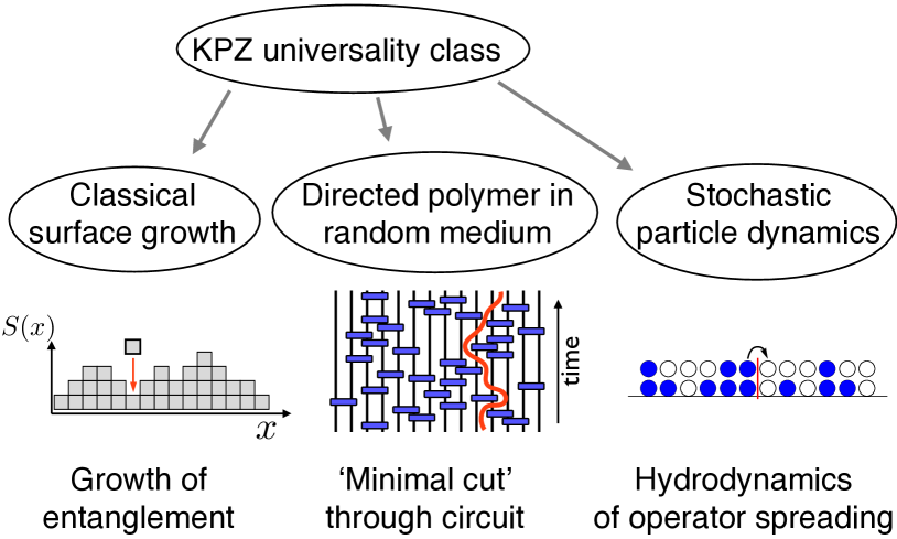
The KPZ universality class also includes two other classical problems besides surface growth Kardar et al. (1986); Huse et al. (1985), as summarized in Fig. 1. We show that each one provides a useful perspective on entanglement dynamics. They are the statistical mechanics of a directed polymer in a disordered potential landscape Huse and Henley (1985), and 1D hydrodynamics with noise (the noisy Burgers equation Forster et al. (1977)). Remarkably, entanglement growth can be related to all three of the classical problems in in Fig. 1, which are sometimes referred to as the ‘KPZ triumvirate’ Halpin-Healy (1998).
In the quantum setting, the directed polymer is related to the ‘minimal cut’, a curve in space-time which bisects the unitary circuit representing the time evolution. This is reminiscent of the Ryu-Takayanagi prescription for calculating the entanglement entropy of conformal field theories in the AdS-CFT correspondence, which makes use of a minimal surface in the bulk space Ryu and Takayanagi (2006), and analogous results for certain tensor network states Swingle (2012); Pastawski et al. (2015); Hayden et al. . Here however the cut lives in spacetime rather than in space, and its shape is random rather than deterministic. (For a different use of the idea of a minimal cut in spacetime, see Ref. Casini et al. .) This picture is more general than the surface growth picture, as it allows one to consider the entropy for any bipartition of the system. It also allows us to generalize from 1D to higher dimensions. In spacetime dimensions the minimal cut becomes a -dimensional membrane pinned by disorder. This picture allows us to pin down approximate critical exponents for noisy entanglement growth in any number of dimensions.
This picture also leads to a conjecture for entanglement growth in systems without noise, both in 1D and higher dimensions, as we discuss below. According to this conjecture, the calculation of the entanglement in higher dimensions reduces to a deterministic elastic problem for the ‘minimal membrane’ in spacetime.
The third member of the triumvirate in Fig. 1 is a noisy hydrodynamic equation describing the diffusion of interacting (classical) particles in 1D. We show that this can be related to the spreading of quantum operators under the unitary evolution, giving a detailed treatment of the special case of stabilizer circuits. Note that while the minimal cut picture generalizes to higher dimensions, the KPZ and hydrodynamic pictures are special to 1D.
We propose that noisy dynamics are a useful toy model for quantum quenches in generic (non-integrable, non-conformally–invariant) systems, even without noise. The logic of our approach is to pin down the universal behaviour of noisy systems (Secs. II—VI), to establish simple heuristics capturing this behaviour (Secs. III, IV), and then to draw conclusions that are likely to be true even without noise (Secs. V, VIII). While the detailed physics of entanglement fluctuations certainly relies on noise, the coarser features of the dynamics — i.e. the leading order time dependence of the entanglement entropy and mutual information — is in fact deterministic. We conjecture that this leading order behaviour (as captured by the directed polymer and hydrodynamic pictures) carries over to Hamiltonian dynamics without noise. On the basis of this we address (Sec. V) some features of entanglement growth that have previously been unclear. We argue that in generic 1D systems the entanglement growth rate can be interpreted as a well-defined speed , but that this speed is smaller than another characteristic speed, which is the speed at which quantum operators spread out under the dynamics. This difference is related to the failure of pictures for entanglement growth in terms of independently spreading operators. We discuss the meaning of . In Sec. VIII we discuss the geometry-dependence of the dynamical entanglement in higher-dimensional systems.
II Surface growth in 1D
We begin by studying entanglement growth under random unitary dynamics in one dimension. After summarizing the KPZ universal behavior, we derive this behaviour analytically in a solvable model, using a mapping to a classical surface growth problem. In the following sections we provide more general perspectives on this universal behaviour by relating the ‘minimal cut’ bound on the entanglement to the classical problem of a directed polymer in a random environment, and by relating the spreading of quantum operators to a 1D hydrodyamics problem.
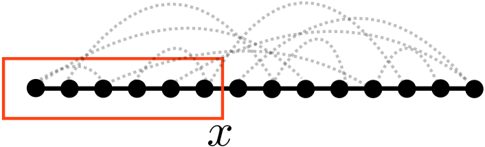
Consider a chain of quantum spins with local Hilbert space dimension (for example spin–1/2s with ). We take open boundary conditions, and label the bonds of the lattice by . We consider only unitary dynamics, so the full density matrix represents a pure state. For now we consider the entanglement across a single cut at position ; we will generalize to other geometries later in the paper. The reduced density matrix is defined by splitting the chain into two halves at and tracing out the left-hand side (Fig. 2). The th Renyi entropy for a cut at is defined as
| (1) |
Logarithms are taken base . In the limit the Renyi entropy becomes the von Neumann entropy,
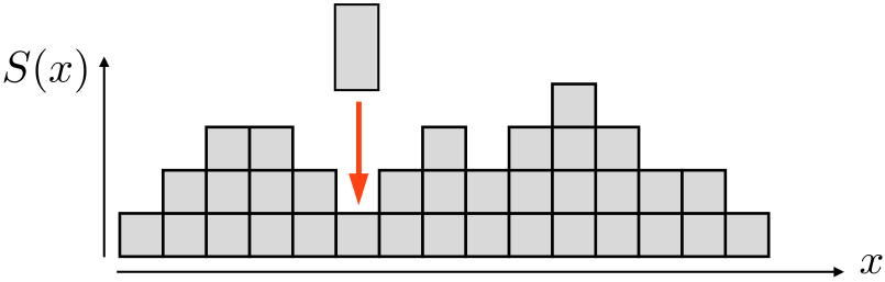
| (2) |
A basic constraint on the von Neumann entropy is that neighboring bonds can differ by at most one111This follows from subadditivity of the von Neumann entropy.:
| (3) |
In this section we focus on the growth of the bipartite entropies with time, starting from a state with low entanglement. (Here , without a subscript, can denote any of the Renyi entropies with .) For simplicity we take the initial state to be a product state, but we expect the same long-time behaviour for any initial state with area-law entanglement.222The setup with area-law entanglement in the initial state is analogous to a quantum quench which starts in the ground state of a non-critical Hamiltonian. We briefly consider initial states with non-area-law entanglement in Sec. IX. We will argue that for noisy unitary dynamics, the universal properties of are those of the Kardar–Parisi–Zhang equation:
| (4) |
This equation was introduced to describe the stochastic growth of a 1D surface or interface with height profile Kardar et al. (1986). It captures an important universality class which has found a wealth of applications in classical nonequilibrium physics, and its scaling properties have been verified in high-precision experiments Takeuchi and Sano (2012); Takeuchi et al. (2011). The constant in Eq. 4 contributes to the positive average growth rate, while is noise which is uncorrelated in space and time. The term describes diffusive smoothing of sharp features. The nonlinear term, with coefficient , describes how the average growth rate depends on the slope; the negative sign is natural here, as discussed in Sec. II.1.3 (and implies that in Eq. 6 below is positive).
KPZ scaling is characterized by an exponent governing the size of fluctuations in the interface height, an exponent governing spatial correlations, and a dynamical exponent determining the rate of growth of the correlation length ( by a scaling relation). These are known exactly Kardar et al. (1986):
| (5) |
In our context the height of the surface is the bipartite entanglement . This is a random quantity which depends on the realization of the noise in the quantum dynamics. The mean height/entanglement grows linearly in time, with a universal sub-leading correction:
| (6) |
Angle brackets denote an average over noise. The fluctuations grow as
| (7) |
We will refer to as the ‘width’ of the surface. The ratio is universal (the constants and are not). The spatial correlation length grows with time as
| (8) |
and the equal time correlation function has the scaling form
| (9) |
On length scales , the surface profile resembles the trace of a 1D random walk: this is consistent with the exponent .
At short times the entanglement growth is affected by initial conditions, while on very long timescales, of the order of the system size, the entanglement saturates. The formulae (6)—(9) apply prior to this saturation. In a finite system the asymptotic profile is that of a pyramid, with a maximum at height , whose height is , minus an correction Page (1993); Nadal et al. (2011). This profile is reached at a time
| (10) |
with bonds closer to the boundary saturating sooner (Secs. III, V). Saturation is also captured in the surface growth description, once we note that there are Dirichlet boundary conditions on the entropy: .
Note that the scaling described in Eqs. 6, 8 implies the existence of two distinct diverging lengthscales during entanglement growth. The fact that is of order implies that spins are entangled over distances of order . In fact we will show in Sec. V that is a sharply defined lengthscale. But prior to saturation, the relevant lengthscale for spatial variations in is parametrically smaller than , namely .
Before deriving KPZ for entanglement, let us briefly consider the status of this equation. At first sight we might try to justify this description of simply on grounds of symmetry and coarse graining. If we were describing classical surface growth, we would appeal to translational symmetry in the growth direction () in order to restrict the allowed terms, and would note that the right-hand-side includes the lowest–order terms in and . But for entanglement we cannot rely on this simple reasoning. First, the transformation is not a symmetry (or even a well-defined transformation) of the quantum system. More importantly, it is not clear a priori that we can write a stochastic differential equation for alone, since the full quantum state contains much more information than . Despite these differences from simple surface growth, we will show that the above equation does capture the universal aspects of the entanglement dynamics.
In the next section we exhibit a solvable quantum model which maps to a classical surface growth problem that is manifestly in the KPZ universality class. Then in the two following sections we give heuristic arguments for more general systems by making connections with the other members of the KPZ triumvirate. Together with the results for the solvable model, these arguments suggest that KPZ exponents should be generic for entanglement growth in any quantum system whose dynamics involves time-dependent randomness. In Sec. VI we perform numerical checks on KPZ universality for quantum dynamics in discrete time.
II.1 Solvable 1D model
We now focus on a specific quantum circuit model for the dynamics of a spin chain with strong noise. We take random unitaries to act on pairs of adjacent spins (i.e. on bonds) at random locations and at random times, as illustrated in Fig. 3. For simplicity we discretize time and apply one unitary per time step. (Dynamics in continuous time, with unitaries applied to the links at a fixed rate in a Poissonian fashion, are equivalent.) We choose the initial state to be a product state, with for all and . We choose the unitaries from the uniform (Haar) probability distribution on the unitary group for a pair of spins, . This model is solvable in the limit of large local Hilbert space dimension .

II.1.1 Dynamics of Hartley entropy
A useful starting point is to consider the limit of the Renyi entropy, . This is known as the Hartley entropy, and quantifies (the logarithm of) the number of nonzero eigenvalues of the reduced density matrix. Equivalently, the Hartley entropy determines the necessary value of the local bond dimension in an exact matrix product representation Verstraete et al. (2008); Perez-Garcia et al. (2007) of the state:
| (11) |
Like the von Neumann entropy, the Hartley entropy of neighboring bonds can differ by at most one:
| (12) |
Recall that logarithms are base . For the present we keep finite.
For the random dynamics described above (Sec. II.1), the Hartley entropy obeys an extremely simple dynamical rule. In a given time step, a unitary is applied at a random bond, say at . Applying this unitary may change the Hartley entropy across the bond ; the entropy remains unchanged for all other bonds. The rule for the change in is that, with probability one, it increases to the maximal value allowed by the general constraint (12):
| (13) |
This ‘maximal growth’ of occurs with probability one when all unitaries are chosen randomly. Fine-tuned unitaries (e.g. the identity) may give a smaller value, but these choices are measure zero with respect to the Haar distribution.
We present a rigorous proof of Eq. 13 in Appendix A. The appendix also gives a heuristic parameter-counting argument which suggests the same result, but as explained there the more rigorous argument is necessary.
The dynamical rule in Eq. 13 defines a simple but nontrivial stochastic process. Before discussing its properties, we use Eq. 13 as a starting point to show that in the limit of large Hilbert space dimension the von Neumann entropy (and in fact all the higher Renyi entropies) obeys the same dynamical rule. The von Neumann entropy is of more interest than , since the latter behaves pathologically in many circumstances333This is because it simply counts up all the (nonzero) eigenvalues in the spectrum of , regardless of how small they are. For example, Hamiltonian dynamics in continuous time — as opposed to unitary circuits like the above — will generally give an infinite growth rate for , in contrast to the finite growth rate for and the higher Renyi entropies..
II.1.2 Limit of large Hilbert space dimension
The present quantum circuit dynamics lead to a solvable model in the limit of large local Hilbert space dimension, . In this limit all the Renyi entropies obey the dynamical rule in Eq. 13.
To show this we consider the reduced density matrix for a cut at , where is the bond to which we are applying the unitary in a given time step. We may write in terms of and the applied unitary matrix. Averaging over the choice of this unitary, we then obtain:
See App. B for details. In terms of the second Renyi entropy this is:
| (14) |
The general constraint allows us to write
| (15) |
with . We now use Eqs. 13, 14 to show that is infinitesimal at large . Rewriting Eq. 14 in terms of , and substituting Eq. 13, immediately shows
| (16) |
For a simple bound444For a large system, this bound on will be far from the tightest possible since we have not exploited the large size of the system., define to be the maximal value of in the entire system. The equation above implies
| (17) |
We may iterate this by averaging over successively earlier unitaries:
| (18) |
This shows that as at fixed time , the probability distribution for concentrates on , so that and become equal.
This implies that the entanglement spectrum is flat, so in fact all the Renyi entropies obey Eq. 13 for the application of a unitary across bond .
II.1.3 Properties of the solvable model
The dynamical rule we have arrived at for the bipartite von Neumann and Renyi entropies at large ,
| (19) |
defines a stochastic surface growth model in which is always an integer-valued height profile (Fig. 4). The remaining randomness is in the choice of which bond is updated in a given time step. At each time step, a bond is chosen at random, and the ‘height’ is increased to the maximal value allowed by the neighbors. Fig. 5 gives examples of local configurations before and after the central bond is updated.
This model is almost identical to standard models for surface growth Meakin et al. (1986); Kim and Kosterlitz (1989). It is in the KPZ universality class (it is straightforward to simulate the model and confirm the expected KPZ exponents) and some non-universal properties can also be determined exactly. Note that the boundary conditions on the right and the left, and the restriction , imply that the entanglement eventually saturates in the expected pyramid profile.
When we move to the continuum (KPZ) description of the interface (4) the nonlinear term appears with a negative sign, meaning that entanglement growth is slower when the coarse-grained surface has a nonzero slope. This is natural given the microscopic dynamics: if the slope is maximal in some region, local dynamics cannot increase the entropy there.
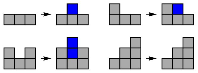
In the present model the difference in height between two adjacent bonds is either or . At early stages of the evolution both possibilities occur. However one may argue that the ‘flat points’, where , become rarer and rarer at late times.555Flat points can disappear by ‘pair annihilation’ (Fig. 5, top left), and can diffuse left or right (Fig. 5, top right), but cannot be created. As a result their density decreases with time. At late times the model therefore becomes equivalent to the well-known ‘single step’ surface growth model Meakin et al. (1986), in which only. An appealing feature of this model is that, for a certain choice of boundary conditions,666The solvable case corresponds to choosing periodic BCs in the classical problem. (These BCs are useful for understanding the classical model, but they do not have an interpretation in terms of entanglement.) In this setting the mean height grows indefinitely, but the probability distribution for the height fluctuations reaches a well-defined steady state. the late-time probability distribution of the growing interface can be determined exactly Meakin et al. (1986). This shows that on scales smaller than the correlation length (and prior to saturation) the interface looks like a 1D random walk with uncorrelated steps. In addition to confirming the expected KPZ exponent , this allows the mean growth rate of the surface to be calculated. After rescaling time so that one unit of time corresponds to an average of one unitary per bond, this gives an entanglement growth rate (6) of .
The mapping to surface growth gives us a clean derivation of universal entanglement dynamics in a solvable model. However this surface growth picture is restricted to the entropy for a single cut (as opposed to the entropy of a region with multiple endpoints) and to one dimension. It will be useful to find a more general language which extends the above results. To do this we now make a connection with the second member of the KPZ triumvirate (Fig. 2), the statistical mechanics of a polymer in a random environment.
III Directed polymers & min–cut
In this section we relate the dynamics of to the geometry of a ‘minimal cut’ through the quantum circuit which prepares the state (Fig. 6). This provides an alternative perspective on the exact result (19) for the solvable model, and also a useful heuristic picture for noisy quantum dynamics in general. This line of thinking reproduces KPZ behaviour in 1D. Importantly, it also allows us to generalize to higher dimensions and to more complex geometries.
Our starting point is the minimal cut bound for tensor networks. This very general bound has been related to the Ryu-Takayanagi formula for entanglement in holographic conformal field theories Ryu and Takayanagi (2006); Swingle (2012); Pastawski et al. (2015); Hayden et al. , and has also been applied to unitary networks as a heuristic picture for entanglement growth Casini et al. .
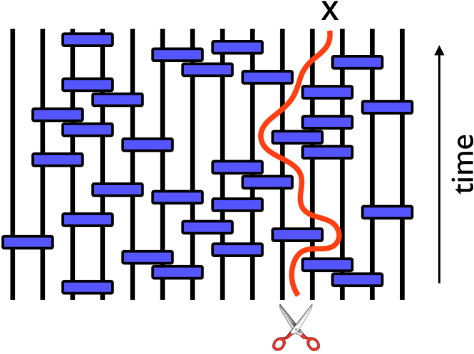
Consider again a random quantum circuit in 1+1D, and a curve like that in Fig. 6 which bisects the circuit and divides the physical degrees of freedom into two at position . Any such curve gives an upper bound on the entanglement: all the Renyi entropies satisfy , where is the number of ‘legs’ that the curve passes through. (This is because the rank of the reduced density matrix is at most .777This can be seen by writing the density matrix in terms of a sum over the indices on the cut bonds.) The best bound of this type is given by the minimal cut, which passes through the smallest number of legs. We denote the corresponding estimate for the entropy . If the geometry of the circuit is random, and the corresponding curve are also random.
In the solvable large model, in fact gives the von Neumann entropy exactly. This follows straightforwardly from the results of the previous section (see below). In a typical microscopic model, on the other hand, is only a bound on the true entropy. Nevertheless we conjecture that the following is generally valid as a coarse-grained picture: i.e. that it correctly captures the universal properties of the entanglement dynamics. This conjecture is equivalent to the applicability of the KPZ description to generic noisy systems; further evidence for the latter is in Secs. IV, VI.
The problem of finding the minimal curve is a version of a well studied problem in classical statistical mechanics, known as the directed polymer in a random environment or DPRE Huse and Henley (1985); Kardar (1985). Here the polymer is the curve which bisects the circuit, and its energy is equal to , the number of legs it bisects. The spatial coordinate of the polymer’s upper endpoint is fixed at , while the lower endpoint is free. Finding is equivalent to finding the minimal value of the polymer’s energy. This corresponds to the polymer problem at zero temperature; however the universal behaviour of the DPRE is the same at zero and at nonzero temperature.888For any finite temperature, the DPRE flows under renormalization to a zero temperature fixed point at which temperature is an irrelevant perturbation.
DPRE models with short-range-correlated disorder are in the same universality class as the KPZ equation Kardar et al. (1986). Let be the minimal energy of the polymer in a sample of height . We may increase by adding an additional layer to the top of the sample. can then be expressed recursively in terms of for the various possible values of . In the continuum limit, this leads to an equation for which is precisely the KPZ equation Kardar et al. (1986). The KPZ exponents given in Sec. II may therefore be applied to the energy of the polymer. The exponent also determines the lengthscale for transverse fluctuations of the polymer:
| (20) |
Since in our case the minimal is simply , we find that the latter executes KPZ growth. In the light of the previous section, this is not surprising. In fact in our solvable model, is exactly equal to the true entanglement entropy (in the large limit). This follows from the fact that the recursive construction of described above precisely matches the large dynamics of Eq. 19. Examples of non-unitary tensor networks in which the minimal cut bound becomes exact are also known Pastawski et al. (2015), including a large-bond-dimension limit similar to that discussed here Hayden et al. .
The utility of the DPRE picture is that it is far more generalizable than the surface growth picture, which is restricted to the entropy across a single cut in 1D. As noted above, the value of in a given microscopic model is typically not equal to any of the physical entropies with . Nevertheless we conjecture that the DPRE and KPZ pictures are valid universal descriptions for all noisy models, so long as they are not fine tuned or nonlocal. This includes Hamiltonian dynamics in continuous time; we discuss this case further in the Outlook section.
III.1 Saturation in the minimal cut picture
Eq. 20 shows that the coarse-grained minimal cut is essentially vertical (prior to saturation of the entropy): the lengthscale for transverse fluctuations is negligible in comparison with . This leads to an extremely simple deterministic picture for the leading-order behaviour of the entanglement, which we will discuss in more detail in Sec. V. Here we briefly consider the saturation of the entanglement entropy, reproducing behaviour known from other contexts Liu and Suh (2014a); Casini et al. .
The definition of the entanglement growth rate implies that the ‘energy’ of such a vertical cut is to leading order. The entanglement in a finite system grows at this rate until time , when it reaches its saturation value . (Here we are neglecting subleading terms, and assuming .) After this time a vertical cut is no longer favourable: instead the minimal cut exits the circuit via the left-hand side. Its shape is no longer unique, but it can be taken to be horizontal, and it has ‘energy’ . This picture corresponds to a simple scaling form (again, neglecting subleading terms)
| (21) |
with
| (22) |
For a finite interval of length in an infinite system we have instead .
These scaling forms are our first confirmation that is really a speed, as well as a growth rate for the entanglement. We will give an independent derivation of this fact for Clifford circuits in the following section, and we will test the above scaling form numerically in Appendix E. We will discuss the interpretation of further in Sec. V. Note that fluctuations have dropped out of Eq. 21, as a result of considering only the leading order behaviour of . These scaling forms agree with the results for holographic CFTs Liu and Suh (2014a) and with an application of the minimal cut formula to a regular tensor network Casini et al. .
It is straightforward to generalize the directed polymer picture to the entanglement or mutual information of arbitrary regions, and even to higher dimensions. We propose in Secs. V, VIII that this picture in terms of a coarse-grained minimal cut is the simplest way to understand the basic features of the ‘entanglement tsunami’ for generic many-body systems, with or without noise.
IV Hydrodynamics of operator spreading
An alternative way to think about the quantum dynamics is in terms of the evolution of local operators . For example, a Pauli operator initially acting on a single spin (e.g. ; we denote the Pauli matrices by , , ) will evolve with time into an operator which acts on many spins. Operators typically grow ballistically Roberts and D. Stanford (2015), in the sense that the number of spins in the support of grows linearly with .
In this section we relate the growth of the bipartite entanglement to the spreading of operators. We focus on the special case of unitary evolution with Clifford circuits (defined below), but we expect the basic outcomes to hold for more general unitary dynamics. We find that the entanglement growth rate is not given by the rate at which a single operator grows, but is instead determined by collective dynamics involving many operators. Remarkably, in 1D these collective dynamics have a long wavelength hydrodynamic description.
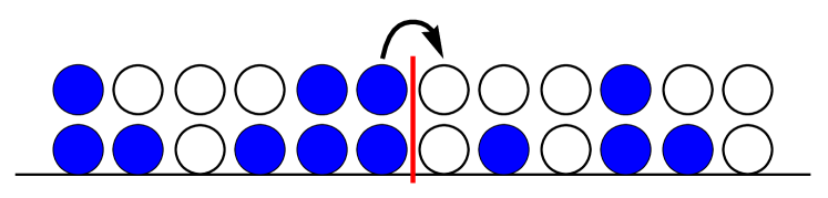
This hydrodynamic description turns out to be the noisy Burgers equation, which is related to the KPZ equation by a simple change of variable and is the final member of the KPZ triumvirate shown in Fig. 1. In the present case the hydrodynamic mode is the density of certain fictitious ‘particles’, shown in blue in Fig. 7. The quantum state is defined by a set of operators (Sec. IV.1) which spread out over time, and the particles are markers which show how far these operators have spread. We will derive their coarse-grained dynamics in Sec. IV.2 after introducing the necessary operator language.
This picture shows that there is a well-defined velocity at which entanglement spreads (at least for the present class of dynamics) and that this is distinct from the velocity governing the growth of operators (Sec. V).
IV.1 Stabilizer operators
It will be convenient to use the language of ‘stabilizer’ operators to describe the entanglement dynamics. We may define the initial state by specifying stabilizers under which it is invariant (in this section we take the number of sites to be ). These operators, denoted () satisfy
| (23) |
For example, if the spins are initially polarized in the direction we may take . At a later time, the above equation still holds, with each stabilizer replaced with the time-evolved stabilizer , where is the unitary operator that evolves the initial state to the state at time .
In the following, we focus on evolution of the initial state with unitary gates in the Clifford group Gottesman (1998). Such gates have recently been used in toy models for many-body localization Chandran and Laumann (2015). The defining feature of Clifford unitaries is that they have a simple action on Pauli operators: single-spin Pauli operators are mapped to products of Pauli operators.
Any product of Pauli matrices can be written as a product of and matrices, so to follow the dynamics of a given stabilizer , we need only keep track of which and operators appear in this product. Furthermore, the overall sign of the stabilizer does not affect the entanglement properties of a system undergoing Clifford evolution, so we do not keep track of it. By writing as
| (24) |
we may specify any stabilizer by a binary vector with components:
| (25) |
For example, the first component of the vector if appears in the product, and otherwise. The binary vector corresponding to a stabilizer is
| (26) |
where the locations of the nonzero elements correspond to and .
We consider the dynamics in two stages. First we consider the evolution of a single operator. Then we will generalize this to understand the dynamics of the state.
How does a single stabilizer evolve? Applying a one or two-site Clifford unitary to corresponds to applying simple local updates to the string . Although the precise details of these updates will not be crucial, we now give some explicit examples of gates which we encounter again in the numerical simulations.
As single-site examples, consider the Hadamard and Phase gates. The Hadamard is a rotation on the Bloch sphere999The rotation is by around the axis. which exchanges the and axes,
| (27) |
so applying a Hadamard to site updates the string by . The Phase gate is a rotation around the axis which maps to
| (28) |
This means that an additional is generated whenever is present in the string, or equivalently . For a two-site example, consider the left and right controlled-NOT (CNOT) gates acting on the leftmost spins in the chain. In the basis, the action of these operators is to flip the ‘target’ spin iff the ‘control’ spin is down:
| (29) | ||||
Conjugating the Pauli matrices by yields:
We see that the operator is added to the string if is present (and similarly for and ). Applying therefore updates by
acts similarly with the roles of the spins reversed.
It is simple to argue that random application of such operations causes the region of space in which is nonzero to grow ballistically. This corresponds to the operator spreading itself over a region of average size , where is the operator spreading velocity. This operator spreading velocity is the analogue, for the present dynamics, of both the Lieb Robinson velocity and the recently discussed ‘butterfly velocity’ Roberts and Swingle in the context of non-noisy systems. The value of depends on the precise choice of dynamics, but it is the same for all initial operators so long as the dynamics (the probability distribution on gates) is not fine-tuned. Further, one may argue that the interior of the region where is nonzero is ‘structureless’. Within the interior, rapidly ‘equilibrates’ to become a completely random binary string.101010Consider the late time dynamics of an operator, or equivalently its string , in an -site system. Random application of Clifford gates gives random dynamics to . It is easy to see that the flat probability distribution on is invariant under the dynamics, regardless of the probabilities with which the gates are applied. By standard properties of Markov processes, this is the unique asymptotic distribution to which the system tends, so long as the choice of Clifford gates is not fine-tuned to make the process non-ergodic. (If the gate set includes each gate and its inverse with the same probability, detailed balance is also obeyed, but this is not necessary.) We expect to equilbrate locally to this structureless state on an timescale, and similarly for the internal structure of operators smaller than .
Now consider the dynamics of a quantum state. Once the sign information in Eq. 24 is dropped, the relevant information in the state is contained in binary vectors corresponding to the stabilizers. We may package this information in a matrix:
| (30) |
Each column corresponds to a stabilizer, and each row to a spin operator or . The dynamical updates correspond to row operations (with arithmetic modulo two) on this matrix. For example, a Hadamard gate exchanges the rows corresponding to and .
A crucial point is that there is a large gauge freedom in this definition of the state. This gauge freedom arises because we can redefine stabilizers by multiplying them together. For example if a state is stabilized by , then it is also stabilized by , and vice versa. This freedom to redefine the stabilizers corresponds to the freedom to make column operations on , or equivalently the freedom to add the vectors modulo two. Note that by making such a ‘gauge transformation’ we may be able to reduce the size of one of the stabilizers, giving a more ‘compact’ representation of the state.
The final fact we need is an expression for the entropy of a region in terms of the stabilizers. Heuristically, this is given by the number of stabilizers that have spread into region from outside. More precisely, define as the number of stabilizers that are independent when restricted to region .111111We truncate all stabilizers to region by throwing away all the spin operators acting outside . In this process some of the stabilizers become trivial, and some become redundant: i.e., equal to products of the others. is the number of stabilizers that are independent when truncated to . Equivalently, is the rank of the matrix after the rows corresponding to the complement of have been deleted; this is how we calculate the entropy numerically for Sec. VI.1. (Independence of the stabilizers corresponds to linear independence of the vectors , with arithmetic modulo two, once they are truncated to region .) The entropy is equal to Hamma et al. (2005a, b)
| (31) |
where is the number of sites in . See Appendix C for a simple derivation of Eq. 31. For Clifford dynamics all Renyi entropies are equal, so we omit the Renyi index on . The maximal value of is , so is bounded by as expected.
This formula has a simple interpretation. In the initial product state we may take one stabilizer to be localized at each site, so and the entanglement is zero. As time goes on, stabilizers that were initially localized outside of grow and enter . Each time a new independent operator appears in , the entanglement increases by one bit. The linear independence requirement in the definition of is crucial, as it leads to effective interactions between the stabilizers which we discuss in the following subsection.
From now on we take to consist of the spins to the right of the bond , and revert to the notation used in the rest of the text for the entanglement across a cut at .
IV.2 Coarse-Grained Operator Dynamics

Each stabilizer (labelled ) has a left and a right endpoint and , marking the extremal spins included in the stabilizer. We view and as the positions of two fictitious particles of type and , represented in white and blue respectively in Figs. 7, 8. There are of each type of particle in total.
In the initial product state, is a single Pauli operator on site , say . This means that each site has one particle and one particle (since ) as shown in Fig. 8 (left). As time increases the particles will typically move to the right and the particles to the left.
The nature of this motion depends on how we define the stabilizers. At first sight the obvious choice is to define as the unitary time evolution of the initial stabilizer, . But in fact it is useful to exploit the gauge freedom in the choice of stabilizers to impose a different ‘canonical’ form. One result of this is that the stabilizers effectively grow more slowly than the velocity (mentioned in the previous subsection) for the spreading of an operator considered in isolation.
Let and be the number of particles of each type at site . The constraint that we impose is:
| (32) |
To see that we can impose this constraint, consider the situation , so that there are three stabilizers that start at . The initial element of each string can be either , , or . If , it is impossible for all three initial elements to be independent. We can then redefine one of the stabilizers, by multiplying it by one or both of the others, in such a way that its length decreases by one.121212By choosing the longer stabilizer we avoid adding length at the right-hand side. Making reductions of this kind wherever possible guarantees that , and also that if , the initial elements of the two stabilizers are distinct. (And similarly for .) With this convention it also follows that : otherwise the operators involved could not commute, which they must.131313Consider the case where : for example let the corresponding stabilizer read . Any stabilizer contributing to must be of the form in order to commute with . By the rule imposed in the text this means that . (The initial stabilizers commute, and this is preserved by the unitary dynamics and the redefinitions of the stabilizers.) Since there are a total of particles which all have to live somewhere, we have Eq. 32.
With this convention, the dynamics of the bipartite entropy is simply related to the hopping dynamics of the particles. By Eq. 32 it suffices to consider only the particles: an particle is just an ‘hole’. We will write the density of particles as . See Fig. 7 for a typical configuration in a subregion of the system.
The utility of the canonical form (32) is that the independence requirement becomes trivial. One can easily check that all the operators which have spread into (the region to the right of ) are independent.141414Consider the stabilizers which act in region , i.e. the stabilizers with . We may argue by contradiction that they remain independent after truncation to subsystem . If not, this means there is some product of the truncated stabilizers which equals one. Let the rightmost spin appearing in any of these stabilizers be . But by our convention for ‘clipping’ the stabilizers, it is impossible for the Pauli matrices acting on spin to cancel out when they are multiplied together. Therefore the operators must in fact be independent. Therefore to find we need only count the number of particles to the right of the cut and subtract the number of sites:
| (33) |
To reiterate, the entanglement increases by one every time an particle drifts rightward across bond (and decreases by one if it drifts across in the other direction).
Now consider the dynamics of the particles. Microscopically, a dynamical time step involves (1) application of a unitary gate, and (2) potentially a ‘clipping’ of stabilizers to enforce the canonical form. Effectively, the particles perform biased diffusion, with the restriction that more than two particles cannot share a site,
| (34) |
This constraint leads to ‘traffic jam’ phenomena familiar from the so-called asymmetric exclusion process Halpin-Healy and Zhang (1995), and to the same continuum description. Our essential approximation is to neglect the detailed internal structure of the stabilizers, and to treat the dynamics of the endpoints as effectively Markovian. We expect this to be valid at long length and time scales for the reason mentioned in the previous subsection: the internal structure of the operators is essentially featureless, and characterized by finite time scales.
We now move to a continuum description. The coarse-grained density obeys a continuity equation
| (35) |
with the particle current. Further, there is a symmetry under spatial reflections, which exchange left and right endpoints (). Writing
| (36) |
where is the deviation from the mean density, the reflection symmetry is
| (37) |
To obtain a long wavelength description, we write the current as a power series in and . Keeping the lowest order terms that respect the symmetry,
| (38) |
These terms have a transparent physical meaning. The drift constant reflects the fact that the average motion is to the right (i.e. operators grow over time). The term is simple diffusion. The noise reflects the randomness in the dynamics. Most importantly, the nonlinear term is the effect of the constraint (32). It reflects the fact that the current is maximal when the density is close to one. The current evidently vanishes when , since there are no particles, but also when (the particles cannot move if the density is everywhere maximal). Therefore we expect .
From the above formulas, the density obeys
| (39) |
known as the noisy Burgers equation Halpin-Healy and Zhang (1995). The entanglement obeys , leading to the KPZ equation:
| (40) |
The sign of is in agreement with that obtained from the surface growth picture in Sec. II and from the directed polymer picture in Sec. III. While we have focussed here on dynamics of a restricted type (Clifford), this derivation of KPZ for entanglement provides independent support for the arguments in the previous sections.
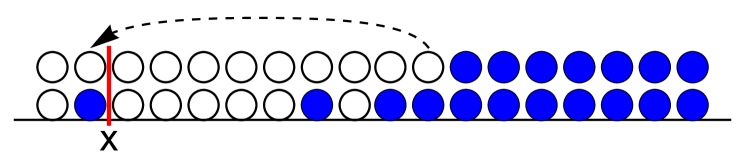
In the language of the particles, the initial state corresponds to uniform density . Saturation of the entanglement corresponds (neglecting fluctuations) to all of the particles accumulating on the right hand side and all of the particles on the left (Fig. 8), i.e to a step function density.
As an aside, it is interesting to consider fluctuations in at late times, i.e. long after the saturation of . Let us revert to our previous notation, where the system has sites and bonds are labelled . Without loss of generality we take . When fluctuations are neglected, the region to the left of is empty of particles, and the entropy is maximal, . Fluctuations will reduce the average. But in order for to fluctuate downward, a blue particle must diffuse leftward from the right half of the system in order to enter the region to the left of , as in Fig. 9. This is a fluctuation by a distance . Such fluctuations are exponentially rare events, because they fight against the net rightward drift for the particles. Thus when is large we expect
| (41) |
Our coarse-grained picture does not determine the numerical constants.
The detailed nature of these exponentially small corrections will differ between Clifford circuits and more general unitary circuits.151515For example in the Clifford case is independent of , while in general the corrections will depend on Nadal et al. (2011). Nevertheless the functional form above agrees with the late time result for generic gate sets, which is simply the mean entanglement in a fully randomized pure state Page (1993); Nadal et al. (2011):
| (42) |
and are the numbers of sites in and its complement.
V The ‘entanglement tsunami’ and the entanglement speed
It is not a priori obvious that the rate governing entanglement growth can be viewed as a speed in generic systems (see Ref. Roberts and Swingle for a recent discussion), although this is known to be the case in holographic CFTs Liu and Suh (2014a). Our results in the directed polymer picture and in the operator spreading picture suggest that is indeed a well-defined speed in generic systems. As we have seen, there is an appealing visual interpretation of this speed as the speed at which the operator endpoints move. However, this speed is smaller than the speed which governs the spreading of an operator considered in isolation: ‘thermalization is slower than operator spreading’.
In our formalism the difference between and arises because in enforcing Eq. 32 we ‘clip’ the stabilizers, reducing their rate of growth. We believe this phenomenon to be general and relevant also to non-noisy dynamics. This picture is contrary to that of e.g. Ref. Ho and Abanin (2015) where the operator spreading velocity is assumed to determine the entanglement growth rate. In the presence of noise, one may also argue that a picture of independently spreading operators underestimates the exponent governing the growth of fluctuations.161616Considering the unitary evolution of a single operator in isolation, its right endpoint executes a biased random walk, traveling an average distance with fluctuations . If we were to neglect the independence requirement in Eq. 31 then the entanglement would be estimated (incorrectly) as the number of independently spreading operators which have reached . The mean of this quantity is and the fluctuations are of order . This is related to the difference between the KPZ universality class of surface growth, which is generic, and the Edwards-Wilkinson universality class which applies when the strength of interactions is fine-tuned to zero Kardar et al. (1986).
The language of a ‘tsunami’ is often used in discussing entanglement spreading, so it is nice to see that — at least in 1D — entanglement spreading can be related to a hydrodynamic problem. In higher dimensions the boundary of an operator has a more complicated geometry, so the hydrodynamic correspondence described above does not generalize.
In order to understand the ‘entanglement tsunami’ better, we now return briefly to the directed–polymer–in–a–random–medium picture developed for noisy systems in Sec. III.
V.1 Simple picture for the entanglement tsunami
When all length and time scales are large, fluctuations in the entanglement are subleading. Neglecting them is equivalent to saying that the ‘coarse-grained’ minimal cut (prior to saturation) is a straight vertical line. This deterministic picture generalizes to the entanglement or mutual information of arbitrary regions, and also to higher dimensions (Sec. VIII). We conjecture that these pictures are valid for the long-time behaviour of entanglement quite generally. The setup relevant to us in the non-noisy case is a quench, in which the initial state is a ground state of one Hamiltonian, and a different Hamiltonian is used for the evolution.
In the 1D case, the deterministic scaling form for the entanglement (of an arbitrary region) which results from the leading-order directed polymer picture is rather simple, and is not new — it agrees with holographic results Liu and Suh (2014a); Leichenauer and Moosa (2015), and as noted in Ref. Casini et al. , can also be obtained from a more microscopic minimal cut picture in which the geometry of the minimal cut is highly non-unique. (We propose that coarse-graining fixes the geometry of the minimal cut; this will be particularly important in higher dimensions.) Here we consider the scaling of the mutual information, in order to clarify the meaning of the speed .
To calculate the entanglement of a region , we must take a cut, or multiple cuts, with endpoints on the boundary points of at the top of the spacetime slice. These cuts can either be vertical, in which case they cost an ‘energy’ (to use the language of Sec. III), or they can connect two endpoints, in which case we take them to be horizontal and to have an energy equal to their length. The entanglement is given by minimizing the energy of the cut configuration. It is a continuous piecewise linear function, with slope discontinuities when the geometry of the minimal cut configuration changes. To generalize the conjecture to systems without noise, we must allow for the fact that the asymptotic value of the entanglement depends on the energy density of the initial state. We therefore replace the entanglement in the formulas with , where is the equilibrium entropy density corresponding to the initial energy density Calabrese and Cardy (2009); Liu and Suh (2014a). This ensures that the entanglement entropy of an -sized region matches the equilibrium thermal entropy when , as required for thermalization. (Heuristically, defines the density of ‘active’ degrees of freedom at a given temperature Roberts and Swingle ).

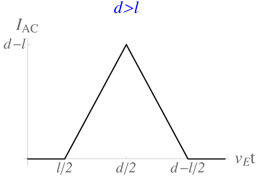

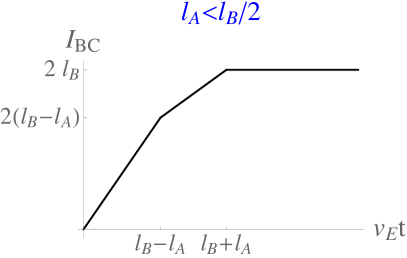

To clarify the meaning of , consider the mutual information between two semi-infinite regions that are separated by a distance (Fig. 10). With the labelling of the regions as in the figure, this is given by
| (43) |
We have for all times, since the appropriate minimal cuts are vertical. If , is given by two vertical cuts, so vanishes. When , is instead dominated by a horizontal cut, so that .
The ‘entanglement tsunami’ is sometimes taken to mean that at time , a ‘boundary layer’ of width inside a given region is entangled with the exterior. If this region were maximally entangled with the exterior, this would reproduce the correct value of the entanglement across a cut (). However this picture is not correct: the result for the mutual information shows that correlations exist over distances up to , not . So although is a speed, it should not be thought of as the speed at which the boundary of the entangled region moves.
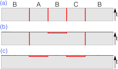
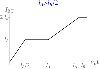
Although the rule for calculating the entanglement is almost trivial, the consequences are not always intuitively obvious. First consider the case where the regions and above are finite rather than infinite (and embedded in an infinite chain); see Fig. 11. When the length of the regions and exceeds their separation , the time-dependence of the mutual information is as shown in Fig. 11. [The sequence of minimal cut configurations required for calculating in this case is (a), (b), (c) shown in Fig. 12.] By contrast, when the separation exceeds the length , the mutual information is always zero (or more precisely, exponentially small171717For a simpler example of exponentially small values of the mutual information, consider at infinite times in a finite system. If the system contains qubits and contains qubits, the mutual information is exponentially small whenever , and given by Eq. 42 as .). [The sequence of cuts for in this case is simply (a), (c)].
Finally, consider the effect of a boundary. Take a semi-infinite chain with regions , , adjacent to the boundary as in Fig. 13 ( is semi-infinite). Consider the mutual information between and , . We must distinguish the case from the case .181818In the former case the first ‘event’ is that the minimal cut at the boundary of goes from being vertical to being horizontal; in the latter the first event is that the two vertical cuts at the boundary of are replaced by a horizontal one. The resulting expressions for are plotted in Fig. 13.
VI Numerical results
We now give numerical evidence that noisy entanglement growth in 1D is in the KPZ universality class. We study the time evolution of spin- chains with open boundary conditions, taking the initial state to be a product state with all spins pointing in the same direction (either the positive or direction) and keeping track of the entanglement entropy across each bond during the evolution. The discrete time evolution is a circuit of one- and two-site unitaries. Fig. [14] shows the structure of a single time step: two layers of 2-site unitaries are applied, one layer on odd and one on even bonds, together with single-site unitaries. Each unitary is chosen independently and randomly (from a certain set specified below). We will use the symbol to denote a generic single-site unitary, and to denote a 2-site unitary.
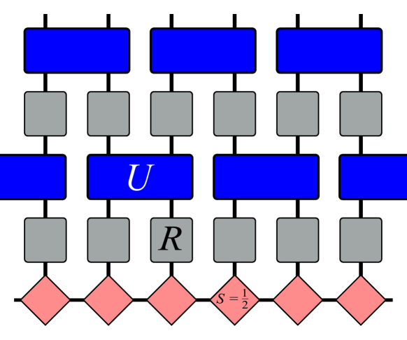
We consider three kinds of dynamics, distinguished by the choice of unitaries. To begin with we study ‘Clifford evolution’ in which the unitaries are restricted to the set of so-called Clifford gates (Sec. IV). Clifford evolution can be simulated efficiently (in polynomial time) using the stabilizer representation discussed in Sec. IV. This allows us to access very long times and to pin down KPZ exponents accurately. Next we study more general dynamics for which polynomial-time classical simulation is impossible, giving evidence that KPZ behaviour holds more generally. The two types of non-Clifford dynamics studied here are referred to as the ‘phase evolution’ and the ‘universal evolution’: details are given below. For these dynamics we use a matrix product representation of the state implemented via iTensor ITe .
The fingerprints of KPZ behaviour that we search for are the two independent critical exponents and (Sec. II). We extract both from the fluctuations in the von Neumann entropy and from the corrections to the mean value (Eqs. 6, 7), and we extract from the spatial correlations in the entanglement at distances shorter than the correlation length (Eq. 9).
VI.1 Clifford evolution
Clifford circuits, or ‘stabilizer circuits’, are a special class of quantum circuits which play an important role in quantum information theory. As shown by Gottesman and Knill, they can be simulated efficiently, even when the entanglement entropy grows rapidly, by representing the quantum state in terms of stabilizers Gottesman (1996): see Sec. IV.
The time evolution operator for a Clifford circuit belongs to the Clifford group, a subgroup of the unitary group on the full Hilbert space. This group may be generated by a small set of local Clifford gates: the two-site controlled NOT gates (Eq. 29) and the single-site Hadamard and Phase gates and (Eqs. 27,28). For circuits built from these gates, time-evolving the state on spins up to a time takes a computational time of order and measuring the entanglement across a given bond in the final state takes a time of order at most. This is in sharp contrast to the exponential scaling which is inevitable for more general circuits.
In all our simulations, each two-site unitary in the circuit is chosen with equal probability from three possibilities: the two types of CNOT gate (Eq. 29) and the identity matrix:
| (44) |
In this section we discuss the simplest Clifford dynamics, which includes only these gates, and no 1-site unitaries (). When the initial state is polarized in the –direction, this set of gates is sufficient to give nontrivial entanglement evolution, with universal properties that turn out to be the same as those for more generic gate sets. We have also studied the ‘full’ Clifford dynamics in which all the Clifford generators are used, choosing the single site unitaries randomly from the three options
| (45) |
Results for this case are similar and are given in Appendix. D.
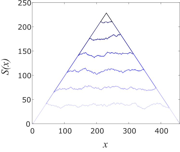
To begin with, Fig. [15] shows the evolution of the bipartite von Neumann entropy (in units of ) for a single realization of the noise (i.e. a particular random circuit) in a system of sites. The curves show successively later times. Note that the entropy saturates more rapidly closer to the boundary, because the maximum entanglement across a bond is proportional to its distance from the boundary. At very late times saturates to a pyramid-like profile representing close-to-maximal entanglement. Our interest is in the stochastic growth prior to saturation, which we will show is KPZ–like. All observables in the following are measured far from the boundary, in order to avoid finite-size effects associated with saturation.
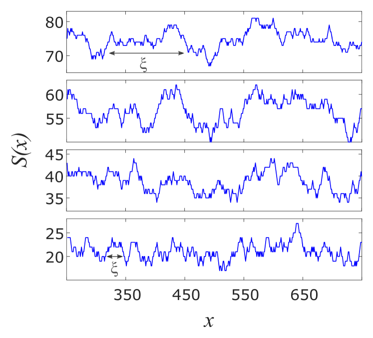
Fig. [16] shows successive snapshots for a subregion of a larger system of bonds (times , from bottom to top). The maximal slope that can appear is 1, in accord with Eq. 3. Note the gradual roughening of the surface and the growing correlation length.
| Evolution type | |||||||
|---|---|---|---|---|---|---|---|
| Clifford | |||||||
| Phase | – | – | – | ||||
| Universal | – | – | – |
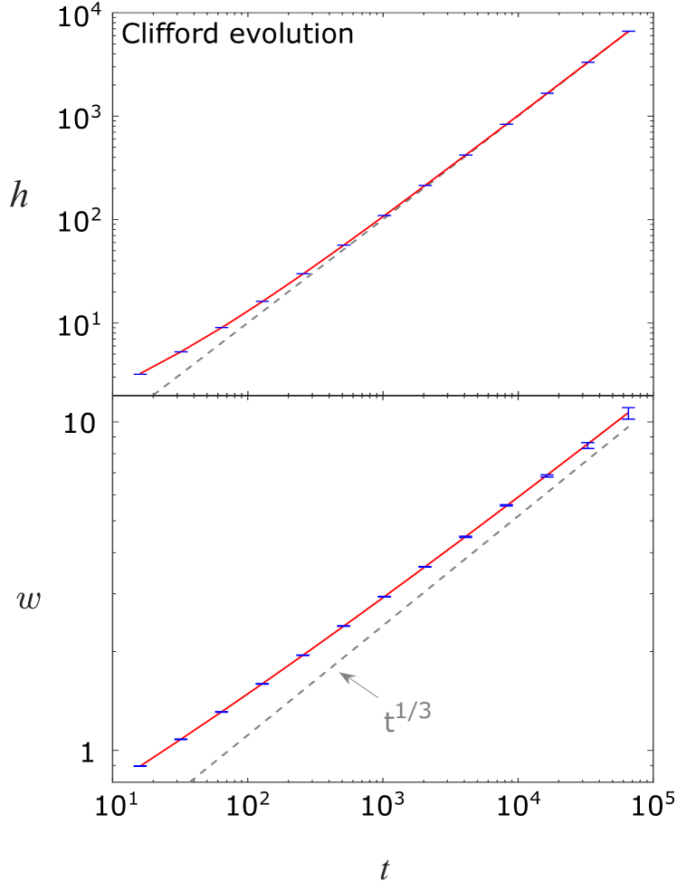
Fig. 17 shows the ‘height’ and ‘width’ of the growing surface,
| (46) |
for very long times. These quantities have been averaged over at least realisations. In each realisation only the entanglement across the center bond is used (therefore all data points are uncorrelated) and the system size is , where is chosen to avoid finite size effects (see Appendix E). We obtain estimates and of the exponent by fitting the data to the expected forms (cf. Eqs.6,7):
| (47) |
Here (with ) captures subleading corrections. We find:
| (48) |
Both estimates of are in excellent agreement with the KPZ value . The solid lines in Fig. 17 show the fits (the fit parameters are in Table 1). The dashed lines show the slopes corresponding to the expected asymptotic power laws, and .
The analysis in Sec. IV implies that is a well-defined velocity, and is a sharply-defined lengthscale characterizing the range of entanglement in the state. We may confirm this by measuring this lengthscale directly. In Appendix E we do this by checking the scaling form for the saturation behaviour of the entanglement given in Sec. III.1.
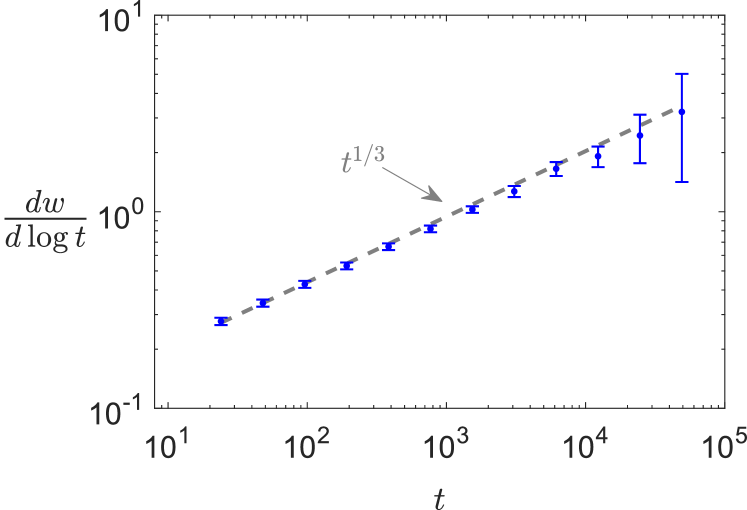
Note the small value of the subleading exponent obtained from the fit. This implies that finite time corrections are reduced if we plot the numerical derivative rather than itself (both quantities scale as at long times). This is done in Fig. 18. The data fits well to the law even at short times. This will be useful for the more general dynamics where long times are not available.
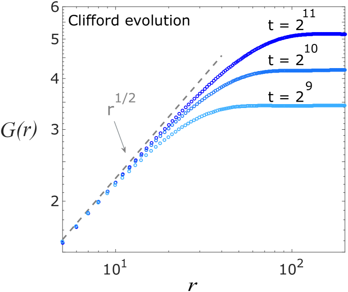
Finally, Fig. 19 shows the spatial correlator defined in Eq. 9, as a function of separation , for three successive times. For small the correlation grows like a with , in agreement with the KPZ prediction for this exponent. For distances , the correlator saturates to a value proportional to . The figure gives an idea of the size of the correlation length for these times.
VI.2 Universal and Phase evolution
The ‘Phase’ and ‘Universal’ dynamics take us outside the Clifford realm, and cannot be simulated efficiently on a classical computer (in polynomial time). We will give evidence that the correspondence with KPZ continues to hold in this more generic situation. However, our results will not be as conclusive as in the Clifford evolution as we will not have access to such long times.
The simulations are performed on spin-1/2 chains of length bonds (501 spins) using the iTensor package ITe . The two types of dynamics are defined as follows. (The 2-site unitaries are always chosen from the set in Eq. 44; the initial state is taken polarized in the -direction.)
Phase evolution: Each single-site unitary is chosen randomly and uniformly from the set of eightfold rotations about the axis in spin space: with .
Universal evolution: This set of gates, unlike the others, is ‘universal’ in the quantum information sense (any unitary acting on the full Hilbert space of the spin chain can be approximated, arbitrarily closely, by a product of gates from this set). The single-site gates include the eightfold rotations mentioned above, together with the Hadamard gate (27). is applied with probability 1/2 and the rotations with probability each.
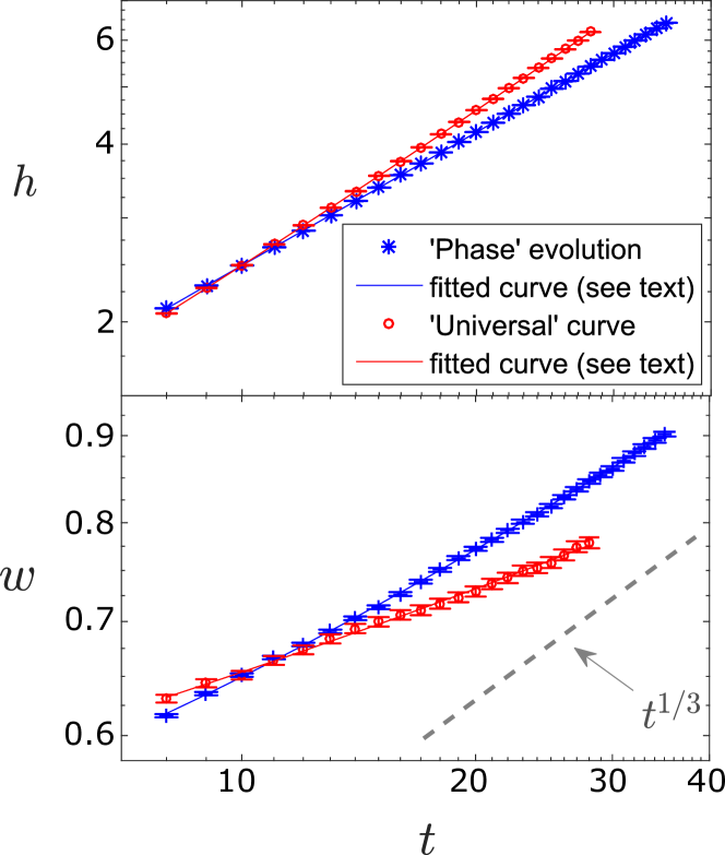
Fig. [20] shows the height and width and for the two protocols (averaged over 380 realisations for the Phase evolution and 200 realisations for the Universal evolution, and over bonds with ). The figure shows fits to the forms in Eq. 47 with and fixed to the KPZ value and fixed to zero (fit parameters are in Tab. 1). The fits with Eq. 47 are consistent with the data. It is not possible to extract precise estimates for from the slope of the log-log plot of , although for the Phase evolution the slope at late times is in reasonable agreement with the expected KPZ value, shown by the dashed grey trendline.
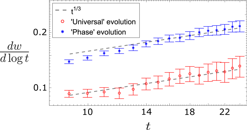
For an alternative attack on we plot the numerical derivative . We found in the Clifford case that the slope of this quantity (when plotted against time on a log-log plot) had smaller finite size corrections than the slope for itself. The corresponding plot is shown in Fig. 21, for times up to (averaging over more than 5000 realisations). The dashed grey lines are the trendlines. Results for both types of dynamics are in good agreement with the expected slope .
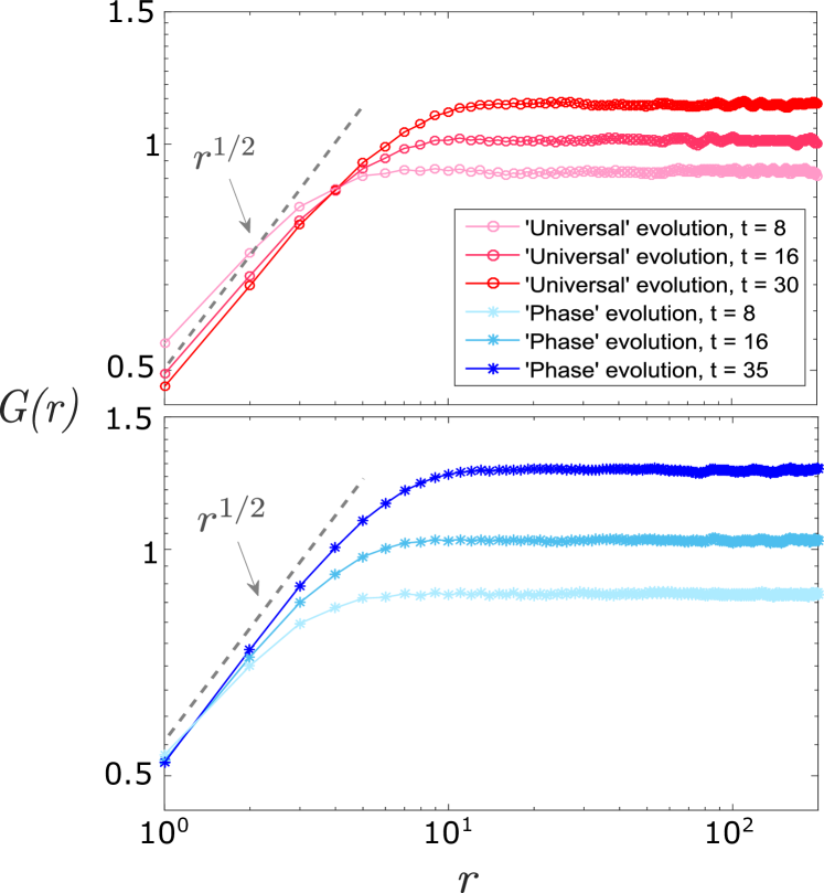
Next we examine the spatial correlator (9) in Fig. 22. For both types of dynamics, the behaviour for agrees well with the KPZ exponent value at the largest available time.
The very long times accessible in the Clifford simulation allowed us to establish KPZ exponents with high accuracy there. For the more generic dynamical rules we cannot reach the same level of precision, but nevertheless the KPZ exponent values are compatible with the data.
Next we briefly discuss a fine-tuned situation in which entanglement dynamics are not KPZ-like: namely when the system is made up of free particles. Then in Sec. VIII we move to higher dimensions.
VII Free fermions are non-generic
The growth of entanglement in systems of free particles is highly non-generic. In the presence of noise the entanglement of a system of free particles on the lattice grows only as , in contrast to the behaviour of generic systems. The case of spatially homogeneous noise has been discussed recently Roósz et al. (2016). The basic point is the same when the noise varies in space: the fact that the single-particle wavefunctions spread diffusively in the presence of noise implies that the entanglement cannot be larger than Roósz et al. (2016).
As a concrete example, consider a short-range hopping Hamiltonian for free fermions,
| (49) |
with noisy matrix elements . For simplicity, take the initial state to consist of particles localized at sites for some set ; for example we could take to consist of all the even-numbered sites:
| (50) |
Under the evolution, each creation operator evolves into a superposition of creation operators,
| (51) |
where is the solution of the time-dependent Schrodinger equation for a particle initially localized at . In the absence of noise, spreads ballistically, but in the presence of noise it spreads only diffusively. The fact that each creation operator is spread out over only sites after a time immediately implies that the mean entanglement is at most of order . (See also Ref. Roósz et al. (2016).) Note however that this argument does not tell us how large the fluctuations are.191919Random unitary evolution of a single wavepacket is discussed in Ref. Saul et al. (1992). However we must consider the full many-body wavefunction, since the formalism of Ref. Peschel (2003) for the free fermion density matrix shows that the initially occupied orbitals do not simply contribute additively to the entanglement.
We have confirmed numerically that for a noisy 1D hopping model, using the formalism of Ref. Peschel (2003) to construct the reduced density matrix. This is much slower than the linear-in-time growth of generic interacting models. The scaling should apply for free fermions in any number of dimensions. In 1D it also applies to certain noisy spin models via the Jordan Wigner transformation: for example the transverse field XY model,
| (52) |
However any generic perturbation to the spin chain spoils the free fermion correspondence. We then expect the generic KPZ behavior to reassert itself.
VIII Higher dimensions
We have discussed several ways of thinking about entanglement growth in 1D. One of these, the directed polymer picture, generalizes naturally to higher dimensions: the polymer is simply replaced by a –dimensional membrane embedded in –dimensional spacetime. As in 1D, we think of this membrane as as a coarse-grained version of a minimal cut bisecting a unitary circuit. The membrane is subject to pinning by ‘disorder’ in space–time arising from the dynamical noise. See Fig. 23 for the two-dimensional case.
We can explore two kinds of question using this picture. First, we can examine universal properties that are specific to the noisy scenario: as in 1D, fluctuations are governed by universal exponents. Second, we can calculate leading order properties of that do not involve fluctuations and which are therefore likely to be valid even in the absence of noise, i.e. for dynamics with a time–independent Hamiltonian. In higher dimensions the behaviour of has nontrivial dependence on the geometry of the region for which we calculate the entanglement. We suggest the ‘minimal membrane in spacetime’ as a simple and general heuristic for such calculations. Below we discuss the case of a spherical region (Sec. VIII.2) and contrast our results with an alternative simple conjecture. For other toy models for entanglement spreading, see Refs. Ho and Abanin (2015); Casini et al. .
Denoting the region for which we wish to calculate the entropy by , and its boundary by , the membrane lives in a spacetime slice of temporal thickness , and terminates at on the upper boundary of this time slice: see Fig. 23. For simple shapes and for times shorter than the saturation time, the membrane also has a boundary on the lower slice, as shown in Figs. 23, 24. In this section we will focus on entanglement growth prior to saturation.
VIII.1 Universal fluctuations of
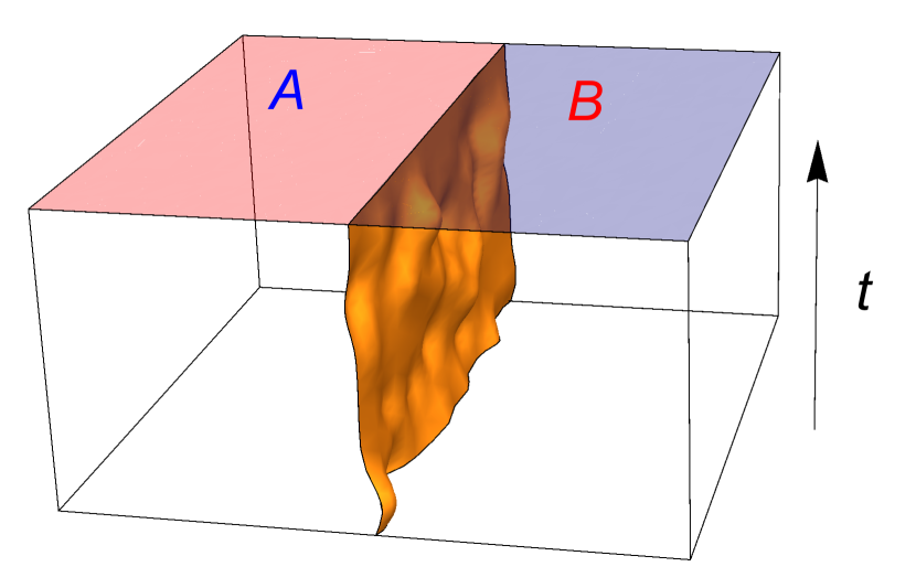
Consider the entanglement for a region whose boundary has length or area . In the case, shown in Fig. 23, is the length of the spatial boundary. Neglecting fluctuations, the ‘world volume’ of the minimal membrane scales as . This gives the leading scaling of the membrane’s energy and hence of the entanglement. As in 1D, subleading terms encode universal data. We now consider these terms.
The pinning of a membrane or domain wall by disorder is well studied Huse and Henley (1985); Nattermann (1985); Kardar (1987); Fisher (1986); Middleton (1995) (a brief summary is in App. F). Translating standard results into the language of the entanglement in a –dimensional noisy quantum system, we find that in both and there is a unique dynamical phase with nontrivial critical exponents. The same is true for continuum systems202020More precisely, for systems with continuous (statistical) spatial translational symmetry. in . However if a lattice is present, two stable phases (and thus a dynamical phase transition) are possible in ; one with nontrivial exponents and one with trivial ones. In the trivial phase the membrane is ‘smooth’ and is pinned by the lattice. In the nontrivial phases the membrane is instead pinned by disorder in a ‘rough’ configuration. We will discuss the nontrivial phases (which are the only ones possible in and for continuum systems in ).
Generally fluctuations have a weaker effect in higher dimensions than in 1D. For simplicity, take a quantum system which is infinite in one direction and of size in the other directions, and consider the entanglement for a cut perpendicular to the infinite direction. Since and its complement are both infinite, will grow indefinitely for this geometry. However there are two regimes, and (here we drop a dimensionful prefactor). For times (see App. F for details):
| (53) | ||||
| (54) |
where the exponent is defined below. This reproduces the 1D result with . Note that when , fluctuations are suppressed with respect to the mean by a factor of : distant regions of the boundary give rise to essentially independent fluctuations which add up incoherently. In the opposite regime , the temporal dimension of the membrane is much larger than its spatial dimensions, so there is a crossover to the 1D directed polymer problem. However, the exponent of the higher dimensional problem appears in the universal dependence of the growth rate:
| (55) |
(The higher corrections will include the term associated with the 1D universality class.) Numerically, the exponent is in , and in Middleton (1995). The subleading exponent in Eq. 53 is negative for , so this correction may be hard to observe numerically.
VIII.2 Minimal membrane picture for dynamics without noise
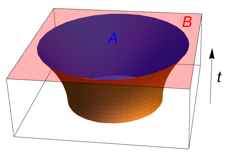
In higher dimensions we can ask how depends on the geometry of region when this geometry is nontrivial. Interestingly, the membrane picture makes predictions about this which do not involve the noise-induced fluctuations, and which are likely also to be valid for Hamiltonian dynamics without noise (with the replacement ) discussed in Sec. V).
As an instructive special case, take to be a disc-shaped region of radius in . (A ball in higher dimensions is precisely analogous.) We assume continuous rotational symmetry, at least on average. At short times, the leading scaling of the entanglement is , since the worldsheet area of the membrane is approximately . However there are corrections to this arising from the curvature of .
We consider the limit of large and large with a fixed ratio . In this regime the effects of fluctuations may be neglected, and instead the energetics of the membrane are determined by deterministic elastic effects. We write the energy of the membrane as
| (56) |
where is the membrane’s area element and is its ‘energy’ density. is got by minimising with appropriate boundary conditions.
Next we Taylor expand in terms of local properties of the membrane. For a flat ‘vertical’ membrane (i.e. with normal perpendicular to the axis) . In general however will depend on the angle by which the surface locally deviates from verticality, as well as, for example, the local curvatures and in the spatial and temporal directions. Using rotational symmetry to parametrise the membrane by the radius ,
| (57) |
However this simplifies in the limit of interest. We first send with fixed. In this limit remains finite but the curvature terms become negligible (see for example the explicit solution below) so we can write . Now we make the second approximation that is small, meaning that we can keep only the correction.
The boundary condition at the top of the spacetime slice is . We will consider times prior to saturation, so the membrane also has a free boundary on . In the relevant limit its ‘energy’ is
| (58) |
Minimal energy requires the boundary condition . When is small we may expand in . This gives , as illustrated in Fig. 24. The corresponding entropy is
| (59) |
This calculation generalises trivially to higher dimensions, where the correction is of the same order. Corrections due to fluctuations come in with negative powers of , and are negligible in the limit we are discussing.
Note that the first correction in the brackets in Eq. 59 is of order , and not of order . This result differs from what one might naively have expected if one guessed that at time an annulus of width inside the disc is entangled with the outside, where is a tsunami velocity. This picture gives an entropy proportional to the area of the annulus,
| (60) |
leading to a negative correction of order . The difference between Eqs. 59, 60 also indicates that a picture in terms of independently spreading operators is misleading, in agreement with what we found in 1D.
In the regime where is of order one, the full dependence of plays a role. This suggests that an infinite number of nonuniversal parameters enter the expression for in this regime, and that there is no general, universal scaling form for the entanglement of a sphere in . However we do expect saturation to remain discontinuous, as in 1D (Eq. 90), occurring via a transition between an optimal membrane configuration which reaches the bottom of the spacetime slice and one (with ) which does not.
IX Outlook
Quantum quenches generate complex, highly entangled states whose dynamics cannot usually be tracked explicitly. For this reason, analytical approaches to quenches have typically relied on additional structure in the quantum dynamics: for example integrability, or absence of interactions, or conformal invariance. This paper has instead studied dynamics that are as unstructured as possible. We propose that noisy dynamics are a useful toy model for quantum quenches in generic (non-integrable, non-conformally–invariant) systems.
Many of our results are of course specific to noisy dynamics: in particular the emergence of KPZ behaviour at long wavelengths in 1D, and the detailed pictures for entanglement growth afforded by the ‘KPZ triumvirate’. But we have suggested that some of our heuristic pictures apply to non-noisy entanglement growth as well (with the replacement mentioned above). We proposed a general directed polymer picture/minimal membrane picture for the scaling of the entanglement/mutual information (Secs. V, VIII.2) and we used the operator spreading picture to clarify the meaning of the ‘entanglement velocity’ and its distinction from the operator spreading velocity (Sec. V). ‘Thermalization is slower than operator spreading’ in generic 1D systems: by contrast this is not true in 1+1D CFTs Calabrese and Cardy (2009), or in certain toy models Ho and Abanin (2015). It would be interesting to make more detailed comparisons with holographic models Liu and Suh (2014a).
Many interesting questions remain. First — within the realm of noisy systems — an analytical treatment for the regime with weak noise would be desirable, i.e. for dynamics of the form
| (61) |
where is a time-independent many-body Hamiltonian, represents noise, and is small. Our conjecture is that KPZ exponents apply for any nonzero value of (unless is fine-tuned) — i.e. that there is no universal distinction between continuous time dynamics and quantum circuits. (Note that there is no distinction between these two cases at the level of conservation laws: once noise is added, energy is not conserved even in the continuous time case.) However our derivations and numerics correspond, roughly speaking, to the large regime. Perhaps the opposite regime could be addressed using a more explicit RG treatment, although it is not obvious how to set this up.
Such an RG treatment might also shed light on the nature of the entanglement spectrum, or equivalently the dependence of on the index . While we believe that all the Renyi entropies execute KPZ growth in the presence of noise, we have not pinned down the –dependence of the various constants. The solvable models suggest that the leading order behaviour may be independent of at large times. What is the appropriate scaling form for the spectrum? Limited timescales prevented us from addressing this numerically (except for Clifford circuits, where all the are trivially equal).
It would also be useful to test the higher-dimensional membrane pictures of Sec. VIII, perhaps exploiting Clifford circuits to reduce the numerical difficulty of higher-dimensional dynamics.
So far we have only discussed initial states with area law entanglement. We may also ask about initial states with, for example, sub-maximal volume law entanglement. The natural expectation (say in 1D) is that the directed polymer picture extends to this case if we glue the unitary circuit to a tensor network representation of the initial state. Then the entropy would include a fluctuating part with KPZ exponents together with a contribution from the initial state.
More speculatively, we may ask whether there exist time-independent Hamiltonians which show KPZ entanglement growth, despite the absence of explicit noise, in some dynamical regimes. This could arise if chaotic dynamics provided effective noise. This seems unlikely on asymptotically long timescales for a generic system, but may hold on intermediate timescales. We may also ask about the structure of the quantum states generated by the random dynamics: in what ways do they differ from ground states of random Hamiltonians, when the amount of entanglement is similar?
Acknowledgements.
We thank M. Kardar for useful discussions. AN and JR acknowledge the support of fellowships from the Gordon and Betty Moore Foundation under the EPiQS initiative (grant no. GBMF4303). SV is supported partly by the KITP Graduate Fellows Program and the DOE Office of Basic Energy Sciences, Division of Materials Sciences and Engineering under Award DE-SC0010526. JH is supported by the Pappalardo Fellowship in Physics at MIT.Appendix A Growth of Hartley entropy in 1D
Consider a one-dimensional quantum spin chain of local Hilbert space dimension , prepared initially in a product state, and apply a sequence of random unitaries that couple two neighboring spins. The location of the local unitary at a given time step is arbitrary. In the following we fix the location of the unitary, but take it to be Haar random.
We prove that in this situation the Hartley entropy generically (i.e. with probability 1) obeys
| (62) |
if a unitary is applied at the bond . The logarithm is of base .
This formula can be interpreted in matrix-product-state (MPS) language. If is the minimal value of the local bond dimension required for an exact MPS representation of the state, then . A heuristic parameter counting argument for the local bond dimension, given in Sec. A.3 below, suggests Eq. 62.
However a more rigorous proof is necessary as such heuristic arguments can fail. In particular, one might naively conjecture a stronger statement: namely that for any state at time , if the unitary at bond is Haar random, then Eq. (62) is true with probability 1. This conjecture is false; a counterexample will be given below in Sec. A.2. We now give a proof of Eq. 62.
A.1 Proof of Eq. (62)
Our genericity proof consists of two parts. First, we will show that given locations of unitaries, there exist certain unitaries such that at each time step, Eq. (62) is true. Second, we will show the negation of Eq. (62)
| (63) |
happens if and only if a system of polynomial equations in the entries of the unitaries is satisfied. (The inequality “” never holds as we noted in the main text.) By the first part of the proof, the zero locus of these polynomial equations does not cover the entire set of unitaries. Therefore it is only a submanifold of strictly smaller dimension, which implies it has measure zero.
For the first part, it is sufficient to consider only three types of local unitaries: the identity , the swap gate , and a unitary with the property that it turns a pair of unentangled polarized spins, , into , a maximally entangled state. Without loss of generality we may take the initial product state to be the polarized state .
We are going to show that using these three types of unitaries at the given locations, one can construct a state whose entanglement entropy is given by Eq. (62). Since Eq. (62) defines the entropy inductively, we only have to show it inductively too.
At , all the spins are unentangled, so we can simply choose for every designated location. Clearly, Eq. (62) is satisfied. At later times, if we do not apply except for unentangled pair of spins, then a spin can be either unentangled or maximally entangled with a single other spin. Therefore, at time the spin that is immediately left to the bond can be
-
(i)
unentangled,
-
(ii)
entangled with a spin to the left of ,
-
(iii)
entangled with the spin that is immediately to the right of the bond , or
-
(iv)
entangled with a spin to the right of .
These are exclusive possibilities, and similarly has four options. Enumerating all 16 cases, which in fact reduces to 7 different cases excluding invalid ones and those related by reflection, one easily checks that there is always a choice among that makes Eq. (62) true. Let us treat three exemplary cases here. If and are entangled at time , then and , so one chooses the identity . If is entangled with a spin on the left of and is entangled with a spin on the right of , then . One chooses the swap to obtain . If and are both unentangled, then one applies the entangling unitary to obtain .
For the second part, recall that for any bipartite state
| (64) |
the number of nonzero Schmidt coefficients is equal to the number of nonzero singular values of the matrix , which is nothing but the rank of . For any positive integer , the rank of is smaller than if and only if every submatrix has determinant zero, i.e., all minors vanish. Thus, a bipartite state having Hartley entropy ( of rank of ) strictly smaller than is expressed by a system of polynomial equations on the coefficients of . If is given by where is a fixed product state, then the coefficients are some polynomials of the entries of the unitaries , and hence the equations that expresses vanishing determinants are polynomial equations in the entries of the unitaries.
Our claim Eq. (62) completely determines the Hartley entropy based on the location of unitaries, and therefore the spatial configuration of the unitaries tells us which minors we should check. Namely, the size of the minors we turn into the polynomial equations is given by (the exponential of) the right-hand side of Eq. (63). In other words, given a spatial configuration of unitaries, the polynomial equations that express Eq. (63) are determined. The polynomial equations are over variables, and the actual number of equations is much larger yet finite. We do not need explicit expressions for these polynomials, only the fact of their existence. These polynomials might a priori read , i.e., they could be trivially satisfied. In that case, the solution to the polynomial equation would be the entire set of unitaries, and Eq. (62) could never be satisfied. However, we just showed in the first part that this cannot happen because there exists a choice of unitaries for which Eq. (62) is satisfied. This implies that the polynomial equations are nontrivial and define a measure zero subset of the entire set of unitaries. This completes the genericity proof.
A.2 Counterexample to the stronger conjecture
We have shown that (62) holds when all unitaries are chosen generically and the initial state is a product state. Naively one might make the stronger conjecture: that the update rule (62) holds whenever a generic unitary is applied to an arbitrary — possibly fine-tuned — state . We construct an explicit which is a counterexample to this stronger conjecture.
Consider four degrees of freedom . The spins and have dimension 2 each, and and have dimension 3 each. (To conform with our consideration of spin chains, the subsystems and should be regarded as subspaces of two or more spin-’s.) The most general form of a quantum state on is
| (65) |
We consider , i.e., is in , where
| (66) |
(This does not give a normalized state, but we are only concerned about ranks.)
The Hartley entropy for the cut is simple to compute. As remarked in the previous subsection, it is the rank of the coefficient matrix. Interpreting this matrix as a linear map, the rank is the dimension of the image of the map from to . The image is precisely the linear span of columns of and . They have three linearly independent columns, implying the Hartley entropy for is . Similarly, the rank of the coefficient matrix for is the dimension of the linear span of the rows of and , which reads 3. That is, the Hartley entropy for is .
If Eq. (62) were to be true for generic choice of Haar random unitary on , then we should be able to find a unitary on such that
| (67) |
We show this cannot hold. Applying the unitary on the state, we obtain
| (68) |
where and are matrices. The coefficient matrix for the cut is then
| (69) |
whose rank should be 6 if . Computing all the minors of the matrix for arbitrary matrices and , we find that all -minors vanish, implying that has rank at most 4. Therefore, for this nongeneric initial state,
| (70) |
A.3 Parameter-counting argument
Consider a 1D state in a matrix product representation. Labelling the states of the qubits (spins) by running from to ,
| (71) |
Since the state is not translationally invariant, we allow the bond dimension to vary from bond to bond (). In an efficient representation, is equal to the rank of the reduced density matrix for a cut at :
| (72) |
We ask how changes when we apply a unitary to the two spins, and , either side of bond . This effects the change (repeated indices summed)
| (73) |
To update the matrix product representation we must find new matrices and which satisfy
| (74) |
In order to solve this equation for and , it will generally be necessary to increase the bond dimension at to a new value . Naively, the necessary value of will generically be determined by equating the number of independent equations in (74) with the number of degrees of freedom in and . (However, the previous subsection shows that this expectation can fail for certain choices of and .)
The number of equations is , since this is the number of possible values for the external indices in (74). The numbers of degrees of freedom in and are and respectively. However, of these are redundant, because the state is unchanged by the transformation , , with an arbitrary matrix. Equating the number of equations with the number of independent degrees of freedom gives
| (75) |
Choosing the smallest solution,
| (76) |
This agrees with Eq. 62 since .
Appendix B Haar average for
Let be the reduced density matrix for a cut at , obtained by tracing out the spins to the left of the cut. Each index on this matrix labels a configuration of the spins to the right of the cut. Let us temporarily label these spins , and let the spin immediately to the left of the cut be denoted . The indices on the reduced density matrices are then:
| (77) |
After applying a unitary on bond ,
Let us average over the choice of unitary, for a fixed initial state:
The Haar average for four elements of a matrix (here , and each index on represents a pair of spin indices) is
| (78) | ||||
The index contractions give the result in the text,
| (79) |
Appendix C Entanglement entropy of stabilizer states
A stabilizer state is a state of an -qubit system defined by a complete set of commuting tensor products of Pauli matrices through equations
| (80) |
The group generated by is naturally called a stabilizer group, and denoted by Gottesman (1996); Calderbank et al. (1997). A trivial example is the all-spin-up state, defined as
| (81) |
for all . The condition that is nonzero and unique is equivalent to the condition that the operator
| (82) |
is a projector of rank one Klappenecker and Rotteler (2002); Linden et al. (2013). Since is in the image of this projector, we see
| (83) |
Since this is a normalized pure density matrix, its trace is equal to 1. But a Pauli matrix has the property that it is traceless. Therefore, only the identity element on the right has nonzero trace:
| (84) |
From this expression, it is straightforward to obtain expressions for reduced density matrices. Suppose the -qubit system is partitioned into two complementary regions and . Tracing out , we have
| (85) |
is nonzero if and only if the tensor component corresponding to is identity, in which case
| (86) |
where denotes the tensor components of corresponding to . The set of all such that can be regarded as a subgroup of , which we denote by . The formula for now reads
| (87) |
It is immediate that is proportional to a projector since it is a sum over a group. It follows that the rank of is equal to . In particular, the (Rényi or von Neumann) entropy of with base-2 logarithm is
| (88) |
The subgroup has period 2, and therefore is an integer, which is equal to the number of independent stabilizers supported only on . This expression for the entanglement entropy has also appeared in Hamma et al. (2005a, b).
Now, regard the stabilizer group as a binary vector space by ignoring the overall phase (sign) factors. Let be the truncation map retaining the components corresponding to the region , and similarly be the truncation map for . It is routine to check that decomposes as for some subspace where and are the spans of stabilizers supported only on and , respectively. Both the truncation maps are injective on . It follows that . This completes the proof of Eq. 31.
Appendix D Numerics for full Clifford evolution
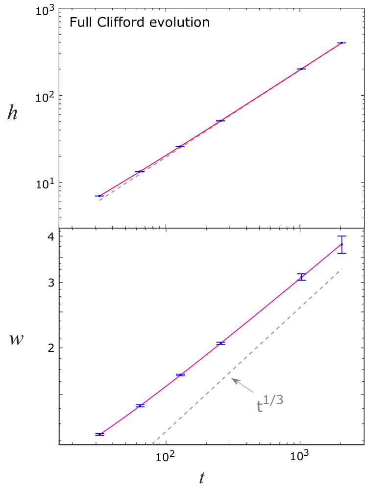
In Sec. VI.1 we have presented numerical results for random unitary evolution using only the CNOT gates Eq. 29. Here we present similar analysis using the full set of generators for the Clifford group showing that the additional gates do not modify the universal behavior. The additional single-site gates are the Hadamard and phase gates defined in Eq. 27 and Eq. 28, respectively (The Hadamard gate corresponds to row swap between and while the phase gates corresponds to adding the vector to the one).
The von Neumann entropy in units of and the corresponding width averaged over realisations (except for the last data point where realisations were used for the average) are plotted in Fig. [25]. The fit to the KPZ universal form Eq. 47 gives and . We also obtain , , , and . These results are consistent with the KPZ universality and with the data presented in Fig. 17.
Appendix E Numerical check that is a speed
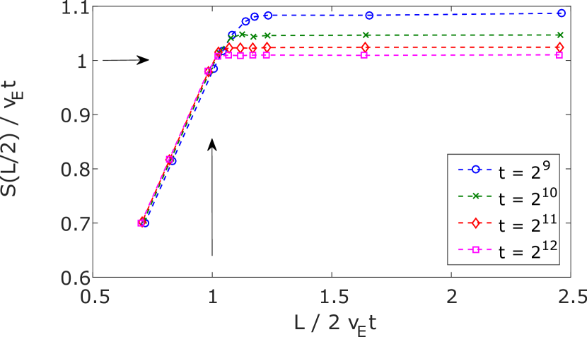
In the main text we have fitted the numerical data points to the form Eq. 47. The parameter quantifies the average entanglement growth rate. We argued in Sec. V that can also be viewed as a velocity associated with entanglement spreading. (This is the speed of the fictitious particles in Sec. IV.) The simplest manifestation of this is in the saturation behaviour of the entanglement. The analytical arguments imply that to leading order (at large and ) the entanglement across a cut at position has the simple scaling form
| (89) |
with
| (90) |
in other words there is no influence of the boundary at times .
In this section we test this conjecture numerically for the Clifford evolution. We set and plot in Fig. 26
| (91) |
as a function of , for several values of the time (). Here is taken from the fits to Fig. 25. According to (89), this plot should converge for large to a plot of against . The results are in excellent agreement with the scaling form, confirming (for the case of Clifford circuits) that is a meaningful velocity.
Appendix F Details of statistics of membranes
The exponents governing the membrane problem are traditionally denoted and , and are related by Huse and Henley (1985). Consider a patch of the membrane with linear dimensions scaling as . This includes both its temporal dimension and its internal spatial dimensions: after a rescaling of time, the membrane is statistically isotropic on large scales. The mean ‘energy’ of this patch of membrane scales as , with fluctuations of order . The lengthscale for wandering of the membrane in the transverse direction is of order . The numerical results quoted in the main text are in good agreement with an epsilon expansion about which gives Fisher (1986) (see also Halpin-Healy (1990)). The scaling forms for the entanglement discussed in the text are easily found by regarding the membrane as made up of patches of appropriate linear size: size for Eqs. 53, 54, and size for Eq. 55.
Note that the geometry of the membrane, including the transverse lengthscale (which is for the regime ) determines the dimensions of the spacetime region around for which the final entanglement is sensitive to small changes in , i.e. in the history of the noise.
References
- Calabrese and Cardy (2005) P. Calabrese and J. Cardy, “Evolution of entanglement entropy in one-dimensional systems,” J. Stat. Mech. 0504, P04010 (2005).
- Calabrese and Cardy (2009) P. Calabrese and J. Cardy, “Entanglement entropy and conformal field theory,” Journal of Physics A: Mathematical and Theoretical 42, 504005 (2009).
- Asplund et al. (2015) C. T. Asplund, A. Bernamonti, F. Galli, and T. Hartman, “Entanglement scrambling in 2d conformal field theory,” Journal of High Energy Physics 9, 110 (2015), arXiv:1506.03772 [hep-th] .
- Hubeny et al. (2007) V. Hubeny, M. Rangamani, and T. Takayanagi, “A covariant holographic entanglement entropy proposal,” Journal of High Energy Physics 2007, 062 (2007).
- J. Abajo-Arrastia and López (2010) J. Aparício J. Abajo-Arrastia and E. López, “Holographic evolution of entanglement entropy,” Journal of High Energy Physics 2010, 1–27 (2010).
- Hartman and Maldacena (2013) T. Hartman and J. Maldacena, “Time evolution of entanglement entropy from black hole interiors,” Journal of High Energy Physics 2013, 1–28 (2013).
- Liu and Suh (2014a) H. Liu and S. J. Suh, “Entanglement tsunami: Universal scaling in holographic thermalization,” Phys. Rev. Lett. 112, 011601 (2014a).
- Liu and Suh (2014b) H. Liu and S. J. Suh, “Entanglement growth during thermalization in holographic systems,” Phys. Rev. D. 89, 066012 (2014b).
- (9) H. Casini, H. Liu, and M. Mezei, “Spread of entanglement and causality,” arXiv preprint arXiv:1509.05044 .
- Fagotti and Calabrese (2008) M. Fagotti and P. Calabrese, “Evolution of entanglement entropy following a quantum quench: Analytic results for the chain in a transverse magnetic field,” Phys. Rev. A 78, 010306 (2008).
- Peschel and Eisler (2009) I. Peschel and V. Eisler, “Reduced density matrices and entanglement entropy in free lattice models,” Journal of Physics A: Mathematical and Theoretical 42, 504003 (2009).
- Buyskikh et al. (2016) A. S. Buyskikh, M. Fagotti, J. Schachenmayer, F. Essler, and A. J. Daley, “Entanglement growth and correlation spreading with variable-range interactions in spin and fermionic tunneling models,” Phys. Rev. A 93, 053620 (2016).
- Lauchli and Kollath (2008) A. M. Lauchli and C. Kollath, “Spreading of correlations and entanglement after a quench in the one-dimensional bose hubbard model,” Journal of Statistical Mechanics: Theory and Experiment 2008, P05018 (2008).
- Kim and Huse (2013) H. Kim and D. A. Huse, “Ballistic spreading of entanglement in a diffusive nonintegrable system,” Phys. Rev. Lett. 111, 127205 (2013).
- Ho and Abanin (2015) W. W. Ho and D. A. Abanin, “Entanglement dynamics in quantum many-body systems,” arXiv preprint arXiv:1508.03784 (2015).
- Bardarson et al. (2012) J. H. Bardarson, F. Pollmann, and J. E. Moore, “Unbounded growth of entanglement in models of many-body localization,” Phys. Rev. Lett. 109, 017202 (2012).
- Serbyn et al. (2013) M. Serbyn, Z. Papić, and D. A. Abanin, “Universal slow growth of entanglement in interacting strongly disordered systems,” Phys. Rev. Lett. 110, 260601 (2013).
- Huse et al. (2014) D. A. Huse, R. Nandkishore, and V. Oganesyan, “Phenomenology of fully many-body-localized systems,” Phys. Rev. B 90, 174202 (2014).
- Chandran and Laumann (2015) A. Chandran and C. R. Laumann, “Semiclassical limit for the many-body localization transition,” Phys. Rev. B 92, 024301 (2015).
- Luitz et al. (2016) D. J. Luitz, N. Laflorencie, and F. Alet, “Extended slow dynamical regime close to the many-body localization transition,” Phys. Rev. B 93, 060201 (2016).
- Verstraete et al. (2008) F. Verstraete, V. Murg, and J.I. Cirac, “Matrix product states, projected entangled pair states, and variational renormalization group methods for quantum spin systems,” Advances in Physics 57, 143–224 (2008), http://dx.doi.org/10.1080/14789940801912366 .
- Islam et al. (2015) R. Islam, R. Ma, P. M. Preiss, M. Eric Tai, A. Lukin, M. Rispoli, and M. Greiner, “Measuring entanglement entropy in a quantum many-body system,” Nature 528, 77–83 (2015).
- Daley et al. (2012) A. J. Daley, H. Pichler, J. Schachenmayer, and P. Zoller, “Measuring entanglement growth in quench dynamics of bosons in an optical lattice,” Phys. Rev. Lett. 109, 020505 (2012).
- Hayden and Preskill (2007) P. Hayden and J. Preskill, “Black holes as mirrors: quantum information in random subsystems,” Journal of High Energy Physics 2007, 120 (2007).
- Sekino and Susskind (2008) Y. Sekino and L. Susskind, “Fast scramblers,” Journal of High Energy Physics 2008, 065 (2008).
- Dankert et al. (2009) C. Dankert, R. Cleve, J. Emerson, and E. Livine, “Exact and approximate unitary 2-designs and their application to fidelity estimation,” Phys. Rev. A 80, 012304 (2009).
- Roberts and D. Stanford (2015) D. A. Roberts and L. Susskind D. Stanford, “Localized shocks,” Journal of High Energy Physics 2015, 1–27 (2015).
- (28) F. G. S. L. Brandao, A. W. Harrow, and M. Horodecki, “Local random quantum circuits are approximate polynomial-designs,” arXiv preprint arXiv:1208.0692 .
- Kardar et al. (1986) M. Kardar, G. Parisi, and Y-C. Zhang, “Dynamic scaling of growing interfaces,” Phys. Rev. Lett. 56, 889–892 (1986).
- Huse et al. (1985) D. A. Huse, C. L. Henley, and D. S. Fisher, “respond,” Phys. Rev. Lett. 55, 2924–2924 (1985).
- Huse and Henley (1985) D. A. Huse and C. L. Henley, “Pinning and roughening of domain walls in ising systems due to random impurities,” Phys. Rev. Lett. 54, 2708–2711 (1985).
- Forster et al. (1977) D. Forster, D. R. Nelson, and M. J. Stephen, “Large-distance and long-time properties of a randomly stirred fluid,” Phys. Rev. A 16, 732–749 (1977).
- Halpin-Healy (1998) T. Halpin-Healy, “Directed polymers versus directed percolation,” Phys. Rev. E 58, R4096–R4099 (1998).
- Ryu and Takayanagi (2006) S. Ryu and T. Takayanagi, “Holographic derivation of entanglement entropy from the anti˘de sitter space/conformal field theory correspondence,” Phys. Rev. Lett. 96, 181602 (2006).
- Swingle (2012) B. Swingle, “Entanglement renormalization and holography,” Phys. Rev. D 86, 065007 (2012).
- Pastawski et al. (2015) F. Pastawski, B. Yoshida, D. Harlow, and J. Preskill, “Holographic quantum error-correcting codes: toy models for the bulk/boundary correspondence,” Journal of High Energy Physics 2015, 1–55 (2015).
- (37) P. Hayden, S. Nezami, X-L. Qi, N. Thomas, M. Walter, and Z. Yang, “Holographic duality from random tensor networks,” arXiv preprint arXiv:1601.01694 .
- Takeuchi and Sano (2012) K. A. Takeuchi and M. Sano, “Evidence for geometry-dependent universal fluctuations of the kardar-parisi-zhang interfaces in liquid-crystal turbulence,” Journal of Statistical Physics 147, 853–890 (2012).
- Takeuchi et al. (2011) K. A. Takeuchi, M. Sano, T. Sasamoto, and H. Spohn, “Growing interfaces uncover universal fluctuations behind scale invariance,” Scientific Reports 1, 34 EP – (2011).
- Page (1993) D. N. Page, “Average entropy of a subsystem,” Phys. Rev. Lett. 71, 1291–1294 (1993).
- Nadal et al. (2011) C. Nadal, S. N. Majumdar, and M. Vergassola, “Statistical distribution of quantum entanglement for a random bipartite state,” Journal of Statistical Physics 142, 403–438 (2011).
- Perez-Garcia et al. (2007) D. Perez-Garcia, F. Verstraete, M. M. Wolf, and J. I. Cirac, “Matrix product state representations,” Quantum Info. Comput. 7, 401–430 (2007).
- Meakin et al. (1986) P. Meakin, P. Ramanlal, L. M. Sander, and R. C. Ball, “Ballistic deposition on surfaces,” Phys. Rev. A 34, 5091–5103 (1986).
- Kim and Kosterlitz (1989) J. M. Kim and J. M. Kosterlitz, “Growth in a restricted solid-on-solid model,” Phys. Rev. Lett. 62, 2289–2292 (1989).
- Kardar (1985) M. Kardar, “Roughening by impurities at finite temperatures,” Phys. Rev. Lett. 55, 2923–2923 (1985).
- Gottesman (1998) D. Gottesman, “The heisenberg representation of quantum computers,” arXiv preprint quant-ph/9807006 (1998).
- (47) D. A. Roberts and B. Swingle, “Lieb-robinson and the butterfly effect,” arXiv preprint arXiv:1603.09298 .
- Hamma et al. (2005a) A. Hamma, R. Ionicioiu, and P. Zanardi, “Bipartite entanglement and entropic boundary law in lattice spin systems,” Phys. Rev. A 71, 022315 (2005a).
- Hamma et al. (2005b) A. Hamma, R. Ionicioiua, and P. Zanardi, “Ground state entanglement and geometric entropy in the kitaev model,” Physics Letters A 337, 22–28 (2005b).
- Halpin-Healy and Zhang (1995) T. Halpin-Healy and Y-C. Zhang, “Kinetic roughening phenomena, stochastic growth, directed polymers and all that. aspects of multidisciplinary statistical mechanics,” Physics Reports 254, 215 – 414 (1995).
- Leichenauer and Moosa (2015) S. Leichenauer and M. Moosa, “Entanglement tsunami in ()-dimensions,” Phys. Rev. D 92, 126004 (2015).
- (52) “ITensor,” http://itensor.org.
- Gottesman (1996) D. Gottesman, “A class of quantum error-correcting codes saturating the quantum hamming bound,” Phys. Rev. A 54, 1862 (1996), quant-ph/9604038 .
- Roósz et al. (2016) G. Roósz, R. Juhász, and F. Iglói, “Nonequilibrium dynamics of the ising chain in a fluctuating transverse field,” Phys. Rev. B 93, 134305 (2016).
- Saul et al. (1992) L. Saul, M. Kardar, and N. Read, “Directed waves in random media,” Phys. Rev. A 45, 8859–8866 (1992).
- Peschel (2003) I. Peschel, “Calculation of reduced density matrices from correlation functions,” Journal of Physics A: Mathematical and General 36, L205 (2003).
- Nattermann (1985) T. Nattermann, “Ising domain wall in a random pinning potential,” Journal of Physics C: Solid State Physics 18, 6661 (1985).
- Kardar (1987) M. Kardar, “Domain walls subject to quenched impurities,” Journal of Applied Physics 61, 3601–3604 (1987).
- Fisher (1986) D. S. Fisher, “Interface fluctuations in disordered systems: expansion and failure of dimensional reduction,” Phys. Rev. Lett. 56, 1964–1967 (1986).
- Middleton (1995) A. A. Middleton, “Numerical results for the ground-state interface in a random medium,” Phys. Rev. E 52, R3337–R3340 (1995).
- Calderbank et al. (1997) A. R. Calderbank, E. M Rains, P. W. Shor, and N. J. A. Sloane, “Quantum error correction and orthogonal geometry,” Phys. Rev. Lett. 78, 405–408 (1997), quant-ph/9605005 .
- Klappenecker and Rotteler (2002) A. Klappenecker and M. Rotteler, “Beyond stabilizer codes ii: Clifford codes,” IEEE Transactions on Information Theory 48, 2396–2399 (2002).
- Linden et al. (2013) N. Linden, F. Matus, M. B. Ruskai, and A. Winter, “The Quantum Entropy Cone of Stabiliser States,” in 8th Conference on the Theory of Quantum Computation, Communication and Cryptography (TQC 2013), Leibniz International Proceedings in Informatics (LIPIcs), Vol. 22, edited by Simone Severini and Fernando Brandao (Schloss Dagstuhl–Leibniz-Zentrum fuer Informatik, Dagstuhl, Germany, 2013) pp. 270–284, 1302.5453 .
- Halpin-Healy (1990) Timothy Halpin-Healy, “Disorder-induced roughening of diverse manifolds,” Phys. Rev. A 42, 711–722 (1990).
