The impact of baryonic physics on the subhalo mass function and implications for gravitational lensing
Abstract
We investigate the impact of baryonic physics on the subhalo population by analyzing the results of two recent hydrodynamical simulations (EAGLE and Illustris), which have very similar configuration, but a different model of baryonic physics. We concentrate on haloes with a mass between and and redshift between 0.2 and 0.5, comparing with observational results and subhalo detections in early-type galaxy lenses. We compare the number and the spatial distribution of subhaloes in the fully hydro runs and in their dark matter only counterparts, focusing on the differences between the two simulations. We find that the presence of baryons reduces the number of subhaloes, especially at the low mass end (), by different amounts depending on the model. The variations in the subhalo mass function are strongly dependent on those in the halo mass function, which is shifted by the effect of stellar and AGN feedback. Finally, we search for analogues of the observed lenses (SLACS) in the simulations, selecting them in velocity dispersion and dynamical properties. We use the selected galaxies to quantify detection expectations based on the subhalo populations in the different simulations, calculating the detection probability and the predicted values for the projected dark matter fraction in subhaloes and the slope of the mass function . We compare these values with those derived from subhalo detections in observations and conclude that the dark-matter-only and hydro EAGLE runs are both compatible with observational results, while results from the hydro Illustris run do not lie within the errors.
keywords:
galaxies: halos - cosmology: theory - dark matter - methods: numerical1 introduction
Numerical simulations of galaxy formation are now able to produce realistic galaxy populations, that reproduce observed relations quite well (Vogelsberger et al., 2014; Schaye et al., 2015). Simulations are fundamental to understand the physical properties that shape galaxies and their evolution; while the cold-dark-matter-only simulations and the treatment of the dark matter component, in general, is well established, there is still not a general consensus on the details of the baryonic physics implementation and differences on this side can lead to quite different predictions in terms of feedback processes and the details of galaxy formation. Moreover, non standard descriptions of the dark matter component, such as warm dark matter (WDM) models, may also have an important impact (Lovell et al., 2012; Lovell et al., 2014; Li et al., 2016).
In this work we analyse the main runs of the EAGLE (Schaye et al., 2015) and Illustris (Vogelsberger et al., 2014) projects, to investigate the effects of different baryonic models on the substructure population. Strong gravitational lensing allows us to detect directly the presence of substructures either via their effect on the relative flux of multiply imaged quasars (Dalal & Kochanek, 2002; Nierenberg et al., 2014) or via their effect on the surface brightness of Einstein rings and lensed arcs (Vegetti & Koopmans, 2009; Vegetti et al., 2010, 2012, 2014; Hezaveh et al., 2016). Numerical simulations can then be used to make predictions for the interpretation of observational results, and possibly rule out dark matter and galaxy formation models.
Previous works concerning subhaloes mainly study cold dark matter-only simulations, whose results are nowadays well established (Giocoli et al., 2008; Springel, 2010). Also, studies investigating in detail subhaloes and their evolution/distribution in different environments and dark matter/hydrodynamical models usually concentrate on Milky Way haloes, aiming to address the well known “missing satellites” and “too big to fail” problems (di Cintio et al., 2011; Di Cintio et al., 2013; Garrison-Kimmel et al., 2014; Wetzel et al., 2016). The aim of this work is to investigate the effect of baryonic physics on the subhalo population concentrating on haloes between and : this corresponds to the halo mass of massive early-type galaxies (ETGs), which act as gravitational lenses in the recent cases of subhalo detections (Vegetti et al., 2010, 2012). In particular, we want to focus on the differences that can arise from different models, stressing the importance of an accurate implementation of baryonic physics.
The paper is structured as follows: we describe the simulations and our halo selection in Section 2. First, we analyse and model the subhalo mass function in the different simulations, concentrating on the difference in the number of subhaloes between the dark matter only and the full hydro runs (Section 3, 4). We proceed by comparing the predictions from simulation with the observational results and what are the probabilities of detecting a substructure given the predictions from different kind of simulations: in Section 5 we select analogues of observed systems and in Section 6 we compare the detection probability inferred from simulations with a real detection in an observational sample (SLACS lenses). In Section 7 we summarise our results. Finally in Appendix A, we point out the differences in the baryonic composition of haloes and subhaloes between the EAGLE and the Illustris simulations. This difference is expected to have an important impact on the gravitational lensing effect of the subhaloes and their detectability. We will investigate this further in a follow-up paper.
2 Simulations
We choose to analyse the main runs of the EAGLE and Illustris simulations for many reasons. The simulations have comparable box sizes, resolutions and starting redshifts; moreover a dark-matter-only counterpart, created with the same initial conditions, exists in both cases and thus constitute an ideal sample for comparison. The main papers from the Illustris (Vogelsberger et al., 2014) and EAGLE (Schaye et al., 2015) collaborations illustrate in detail the differences between the models of baryonic physics, in addition to the differences in the codes - AREPO (Springel, 2010) and a modified version of GADGET3 (Springel et al., 2008), respectively - used to run the simulations. It has been shown that, when looking at the structural properties of haloes in detail, small but significant differences may arise, caused by the simulation code (Heitmann et al., 2008) or even by the halo (Knebe et al., 2011, 2013) and subhalo finders (Onions et al., 2012). These variations become particularly important when we focus on individual structures or small-scale detail. Similar versions of SUBFIND (Springel et al., 2001b) have been used in both simulations to identify structures, eliminating part of these potential differences. Nevertheless, since the baryonic component is treated differently in the two codes, we still expect some effect on the (sub)halo identification. We make use of the existing SUBFIND catalogues of the two simulations and we concentrate in the mass bin of massive early-type galaxies (ETGs). SUBFIND starts the subhalo identification from overdensity peaks within the main halo (see Muldrew et al. 2011 for more details on the algorithm), making it a good candidate for a comparison with the potential corrections used to find subhaloes in gravitational lens systems (Vegetti et al., 2010; Vegetti & Koopmans, 2009).
Due to the resolution limits, the smallest subhaloes have a mass (with at least 10 particles). We include these subhaloes for statistical purposes, but we caution that reliable measurements require a minimum of 100 particles per subhalo (Onions et al., 2012). The cases where particle numbers drop below 100 particles will be marked by a gray region when necessary. Given the good agreement between the two dark-matter-only (hereafter DMO) runs, in this work we show results only from EAGLE for the DMO case. We use different halo mass definitions throughout this work: is defined as the mass of a sphere centered on the halo and enclosing 200 times the critical density (2.77 ) and we chose it as the main halo mass definition since it is more easily comparable to observational results - thus we will refer to this where no other definition is specified ; is the mass of the group in the halo catalogue identified by the FOF algorithm, which has no pre-defined shape and is usually larger than : this method uses a linking length (conventionally set to ) to establish which particles belong to the halo; is defined as the mass within the sphere enclosing the virial overdensity, which is calculated from the spherical collapse model (Bryan & Norman, 1998) and depends on the cosmological model (Sheth & Tormen, 1999; Despali et al., 2016). The last two definitions will be used respectively in Figure 1 - as a general definition to include all haloes and subhaloes in the catalogues - and Figure 6 - for a comparison with the virial masses calculated from the observational data.
We now list the main features of the two simulations.
2.1 EAGLE
In this work we analyse the main run of the EAGLE project, created as part of a Virgo Consortium project called the Evolution and Assembly of Galaxies and their Environment (Schaye et al., 2015; Crain et al., 2015; McAlpine et al., 2016) using a modified version of GADGET-3. (Springel et al., 2008). The EAGLE project consists of simulations of CDM cosmological volumes with sufficient size and resolution to model the formation and evolution of galaxies with a wide range of masses, and also includes a counterpart set of dark matter only simulations of these volumes. The galaxy formation simulations include the correct proportion of baryons and model gas hydrodynamics and radiative cooling and state-of-the-art subgrid models are used to follow star formation and feedback processes by both stars and AGN. The parameters of the subgrid model have been tuned to match some observational results, as the galaxy stellar mass function and the observed relation between stellar and black hole mass (Schaye et al., 2015). The main run and its dark matter only counterpart follow dark matter and (in the first case) gas particles in a box size of 100 Mpc, from redshift to the present time. The cosmological parameters were set to the best fit values provided by the Planck Collaboration et al. (2014) and are: , , , and . With this model, the dark matter particle mass is 1.15 in the DMO run and 9.70 in the full one, while the initial gas particle mass is 1.81 .
The galaxy formation model employs only one type of stellar feedback, which captures the collective effects of processes such as stellar winds, radiation pressure on dust grains, and supernovae, and also only one type of AGN feedback (as opposed to e.g. both a “radio” and “quasar” mode). Thus, as detailed below, it differs from the feedback implementation of the Illustris.
2.2 Illustris
The Illustris Project is a series of hydrodynamical simulations of cosmological volumes that follow the evolution of dark matter, cosmic gas, stars, and super massive black holes from a starting redshift of z = 127 to the present time. In this work, we used the main run Illustris-1 (and the dark matter only run Illustris-1-Dark), which has a box size of 106.5 Mpc and follows dark matter particles and (initial) gas cells. The simulations were run using the recent moving-mesh AREPO code (Springel, 2010). The adopted cosmological model has , , , and , consistent with the WMAP-9 measurements (Bennett et al., 2013). In this case, the dark matter particle mass is 7.5 in the dark matter-only run and 6.3 in the full one, while the initial gas particle mass is 1.3 . The galaxy formation model includes gas cooling (primordial and metal line cooling), a sub-resolution ISM model, stochastic star formation, stellar evolution, gas recycling, chemical enrichment, kinetic stellar feedback driven by SNe, procedures for supermassive black hole seeding, super massive black hole accretion and merging, and related AGN feedback (radio-mode, quasar-mode, and radiative) and some free parameters constrained based on the star formation efficiency in smaller scale simulations (Vogelsberger et al., 2014). This implementation leads to a generally stronger AGN feedback with respect to the one in EAGLE. We made use of the data products and the scripts provided in the Illustris data release (Nelson et al., 2015).
3 The subhalo mass function
The subhalo (and also the halo) mass function has been extensively studied in previous works (Giocoli et al., 2008; Springel, 2010), which made use of dark matter only simulations. It is well established that the presence of baryons modifies the halo structure (Schaller et al., 2015) and may also influence the subhalo population, in terms of their number, spatial and mass distribution. A direct comparison between DMO and hydrodynamical simulations with this purpose can be done by means of zoom-in resimulations (Zhu et al., 2016; Fiacconi et al., 2016) or full cosmological runs (e.g. Sawala et al. 2013) . The first approach allows to reach very high resolutions and thus small subhalo masses, but the results are intrinsically limited in the number of parent haloes and thus do not give statistical predictions on the subhalo mass function, while in the second case there are stronger limitation in resolution; on the other hand, using full cosmological runs guarantees to take into account large scale effect such as the total abundance of haloes. We use the main EAGLE and Illustris runs where the lowest subhalo mass is around ; given their very similar overall configuration, they allow us to directly test how different baryonic physics implementations influence the subhalo mass function.
Generally, the action of baryons on the overall DM distribution in haloes and subhaloes is threefold: reionization affects the formation and evolution of low-mass haloes, making them almost completely dark (with no star formation) for ; the DM concentration in the inner region is increased due to gas cooling and adiabatic contraction, both in the haloes and in the most massive subhaloes which host stars; stellar and AGN feedback cause differences in halo mass, both at the low and high mass end (Cui et al., 2012; Sawala et al., 2013; Vogelsberger et al., 2014; Velliscig et al., 2014; Schaller et al., 2015; Sawala et al., 2015), generally making haloes “lighter” in the hydro runs and thus shifting the halo mass function; finally, different feedback models may affect how matter is stripped from subhaloes. For example, stronger tidal forces in the hydro runs may remove mass more efficiently from subhaloes during their infall (Zhu et al., 2016). Earlier works (Sawala et al., 2013; Schaller et al., 2015; Vogelsberger et al., 2014) showed that the abundances of both haloes and subhaloes are reduced in hydrodynamic simulations compared to the DMO counterparts, as a consequence of a reduction in mass. Nevertheless, the amount of this reduction depends on the baryonic physics model and thus in the following sections we will explore in detail the differences between the EAGLE and the Illustris runs.
3.1 Halo vs. subhalo mass function
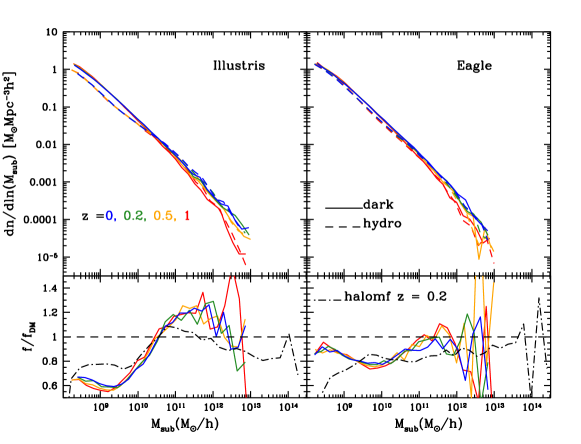
First of all, we want to investigate how the differences in the subhalo population can be related to those in the halo mass function: a different number of haloes available for accretion at redshift would induce a different subhalo mass function at redshift . Figure 1 shows the halo (top panels) and subhalo (bottom panels) mass function for both simulations, at four redshifts between 0 and 1. In the upper panel we plot the halo mass function, using all the haloes in the FOF catalogues and, thus, in this case we choose as halo mass; results from the dark-matter-only and full hydrodynamical run are represented, respectively, with solid and dashed lines. In the small lower panels, we highlight the difference between the two cases: by looking at the fractional difference of halo counts between the hydro and the dark-matter-only run, we notice some similarities and some differences between the two simulations. We observe the predicted reduction of the number of objects from the DMO to the hydrodynamical runs, but while in the EAGLE case, this lack of structures is maintained at all masses (even the AGN feedback cannot expel enough baryons to reduce the halo mass at the high-mass end, so that the ratio tends to 1, as in Schaller et al. 2015), in the Illustris the reduction is not constant and there are more intermediate mass haloes in the hydro run than in the DMO one. This behaviour can be explained as the combined effect of stellar and AGN feedback: they both are less efficient around , leaving these masses unaltered and so increasing their abundance due to the contribution of higher masses that are shifted to these lower values. This is consistent with what is shown in Vogelsberger et al. (2014); indeed Cui et al. (2012); Cui et al. (2014) suggest that neglecting the AGN feedback can lead to an increase of the halo mass function at the massive end.
The second panel of Figure 1 shows the global subhalo mass function, in the same units of the halo mass function. The colour scheme is the same; the dot-dashed black curve in the lower panels shows the fractional change of the halo mass function at from the previous panel, for a more straightforward comparison. We notice a clear relation between the two mass functions: a considerable part of the difference in the subhalo counts between the hydro and dark-matter-only run, can be attributed to the underlying difference in the halo mass function. Having less small structures that can be accreted by larger haloes at any redshift leads to a different number of subhaloes - also enhanced by the fact that not all the small haloes at will be accreted. Nevertheless, the residuals do not correspond exactly, and the additional differences can be attributed to the action of baryonic physics, as cooling, adiabatic contraction and tidal forces inside the halo.

3.2 Mass bins
We select the dark matter haloes with a mass , consistent with the mass range of massive elliptical galaxies with which we will compare further on in this work. In this mass range, the baryonic effect on the halo mass function is similar for the two simulations, leading to a reduction in the number of haloes. The minimum subhalo mass that we show in our plots is , which corresponds to depending on the run. Previous works showed that the subhalo identification may not be reliable with less than 100 particles (Onions et al., 2012), which would correspond to . Here, we keep the small subhaloes in the plots, but we remind that the results for this mass bin must be interpreted with caution. We use only subhaloes with more than 100 particles to fit the mass function.
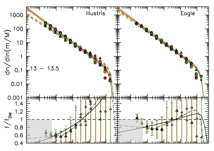
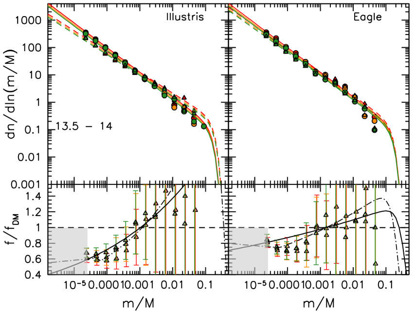
Figure 2 shows the subhalo mass function in three bins of halo mass, for the two simulations and both the dark-mater-only and hydro run. We fit our measurements with the model from Giocoli et al. (2010a):
| (1) |
where the parameters are respectively the slope (assumed negative), the exponential cut-off and the normalization of the curve. We fit the subhalo mass function corresponding to different halo masses and redshifts (as in Figure 2) and then take the average value of the best fit slope. Consistently with previous works, for the dark-matter only case we recover the standard value of ; since the values in Giocoli et al. (2010a) are for virial haloes, the other parameters of our best-fit differ. For the runs with baryons, we find a best fit slope which is less steep than the DMO case (see Table 1) . Note that the fitting functions are shifted vertically by the redshift dependence, and thus the residuals between them shift horizontally in the residual panels, fitting the points well within the errorbars. As can be understood from the lower panels of Figures 1 and 2, the presence of baryons modifies the shape of the subhalo mass function. In order to provide a simple description and be able to compare with observational results (Vegetti et al., 2014), we fit Equation 1 both to the DMO and the hydro runs. However it should be noted that for the latter a single power-law model may not be as accurate for the entire subhalo mass range as for the DMO case. For this reason, we also calculate the best-fit slope separately for two subhalo mass intervals and the best fit values are listed in the third and fourth columns of Table 1. We see that the mass function is steeper for the low-mass subhaloes (when , which corresponds to the plateau in the residual panels of Figure 2) and has a slope similar to the DMO case, consistently with what found in Sawala et al. (2017). The dot-dashed line in the lower panels of Figure 2 shows the ratio between the DMO subhalo mass function and the hydro one which combines the two slopes.
| Subhalo mass function slope | |||
|---|---|---|---|
| sim | |||
| DMO | -0.90 0.03 | - | - |
| EAGLE | -0.85 0.04 | -0.91 0.03 | -0.82 0.06 |
| Illustris | -0.76 0.02 | -0.87 0.03 | -0.72 0.09 |
Different colors stand for different redshifts and the solid black line shows the ratio between the fitting functions. To test whether the residuals depend on the halo mass definition, we re-calculated them also for the whole FOF halo. They behave consistently with those within , showing that the lack of small subhaloes in the simulations does not depend only on the distance from the centre, supporting the point that the variation in the halo mass function may dominate over a faster disruption rate inside the halo.
Looking at the errorbars we notice that the difference in fractions between the two simulations is significant only at the low mass end where the number of objects is high enough and therefore the errorbars are smaller. We will explore the low mass end of the subhalo mass function with higher resolution simulations in a follow-up paper: in order to distinguish between the effect of baryons and those from different models of dark matter (such as warm dark matter) we need a good statistic at .

4 Subhalo counts
In this section we present and model the distribution of subhaloes as a function of radius, both in terms of their three dimensional number density and in projection. As we adopted as halo mass, we use accordingly.

| number density of subhaloes | |||
|---|---|---|---|
| sim | |||
| z = 0.2 | |||
| DMO | (1.79 , 309) | (2.12 , 436) | (1.12 , 881) |
| EAGLE | (1.62 , 330) | (1.92 , 447) | (1.04 , 895) |
| Illustris | (0.732 , 438) | (1.04 , 488) | (1.11 , 760) |
| z = 0.5 | |||
| DMO | (2.74 , 291) | (3.23 , 388) | (1.17 , 381) |
| EAGLE | (2.4 , 306) | (4.38 , 360) | (1.61 , 514) |
| Illustris | (0.732 , 438) | (2.02 , 733) | (2.02 , 677) |
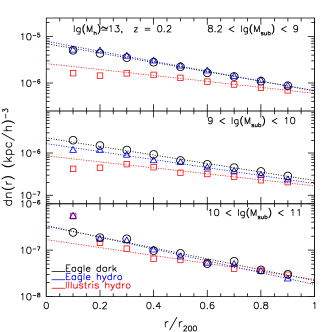
It has been shown in previous works (e.g. Springel et al. 2008) that the number of subhaloes as a function of radius can be well fit by an Einasto profile:
| (2) |
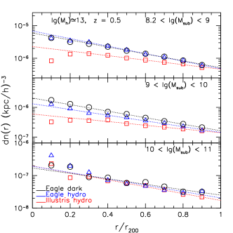
In Figure 3 we show the radial distribution of subhaloes: for each simulation, the distribution of subhaloes can be modelled by the same curve, when the number is normalized by the mean number density of subhaloes in that specific mass bin within . Solid lines show the best fit Einasto profile to the points, while the same fit for (for which we do not show the points) are given by the dashed lines. In all cases, we find that our points are well fitted by an Einasto profiles with , while the values of normalization and scale radius vary with halo mass and redshift. In Table 2 we provide the best-fit values for each combination of redshift, mass bin and simulation. At fixed redshift, increasing the halo mass corresponds to an horizontal shift in the profiles (i.e. an increased number density of subhaloes at large distances); at fixed mass, increasing leads to an increase in the normalization (i.e. an overall increased number density of subhaloes). We also note that for high halo masses, the three profiles have more similar shapes, indicating that the effect of baryons is less important in this mass range.
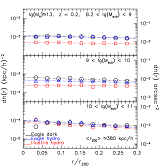
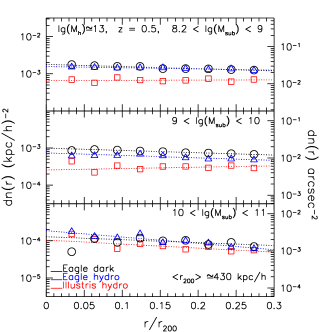
Figure 4 shows the average subhalo counts in units of , and . as a function of distance from the centre in three and two dimensions, for haloes of mass at redshift 0.2 and 0.5; the subhalo counts are averaged over all the haloes in the selected mass bin and over three projections per system for the two dimensional measurements. We compare the dark-matter-only results, the EAGLE (blue open triangles) and the Illustris (red open squares) hydrodynamical simulations. We consider three logarithmic bins in subhalo mass (in : (8.2-9), (9-10) and (10-11). The left panels show the average three dimensional subhalo counts within , expressed as number of subhaloes per . The general trend is very similar for all the simulations, but we note again a different effect of the two models of baryonic physics: in the Illustris simulation, the lack of subhaloes is again more evident than in EAGLE, reflecting what could be inferred from the subhalo mass functions. In projection (right panel), the distributions flatten and the relative behaviour of the three cases is the same, similarly to what found in Xu et al. (2015) - this time we plot only the subhalo counts within , because only the central parts of the halo are relevant for lensing. Projecting all the substructures inside the FOF group gives a slightly different results in the higher subhalo mass bin; this is explained by the fact that bigger subhaloes are found in the outer region of haloes and the FOF group is more extended than .
5 A comparison with observations
5.1 The SLACS survey
The Sloan Lens ACS (SLACS) Survey is an efficient Hubble Space Telescope (HST) Snapshot imaging survey for galaxy-scale strong gravitational lenses (Bolton et al., 2006). The SLACS survey was optimized to detect bright early-type lens galaxies with faint lensed sources in order to increase the sample of known gravitational lenses suitable for detailed lensing, photometric, and dynamical modeling. SLACS has identified nearly 100 lenses and lens candidates, which have a stellar mass ranging from to (Auger et al., 2009) and estimated total masses of the order of (Auger et al., 2010a), at redshift - spanning approximately for the lenses and for the source. They can be considered representative of the population of massive early-type galaxies with stellar masses (Auger et al., 2009).
5.2 Considerations on the IMF
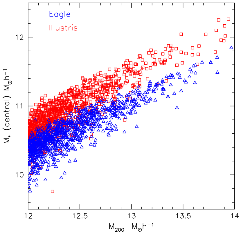
Even though it could seem more straightforward, selecting the simulated galaxies in terms of the total stellar mass may present some problems concerning the chosen IMF: the SLACS total stellar masses have been calculated by Auger et al. (2009), using both the Chabrier and the Salpeter IMF and the latter has been shown to be the preferred model. Auger et al. (2010a) ruled out a Chabrier mass function when calculating the total halo mass (this is also supported by the findings of Grillo et al. (2009). On the other hand, both the EAGLE and Illustris simulations have been run with a Chabrier IMF and rescaling the mass with the usual relation would not yield to a meaningful comparison: changing the IMF in the simulation code would require modification in the baryon and subgrid models, leading to more complicated differences than a simple rescaling. For this reason, following Xu et al. (2016), we avoid a selection by total stellar mass and prefer to use dynamical measurements and velocity dispersion instead. This presents another advantage: as can be seen in Figure 7, the stellar mass of the central galaxy is on average different in the two simulations for a halo of a given total mass and so using it as a main selection criterion could enhance the difference in total mass between the two samples.
5.3 Selection of SLACS analogues
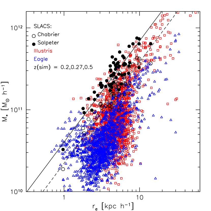
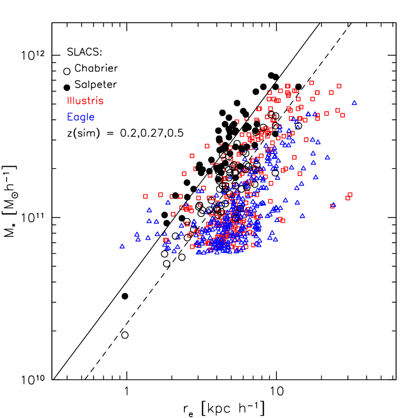
In order to select analogues of the SLACS lenses from the considered simulations, we start by excluding all haloes which are clearly unrelaxed: we exclude those for which the distance between the halo centre of mass and the position of the minimum of the potential is more than 5 of the virial radius, as they may include multiple components and are not suitable for our selection (Neto et al., 2007; Ludlow et al., 2012).The top panel of Figure 5 shows all galaxies selected only by halo mass and relaxation; unlike in previous sections, here we also include haloes with masses lower than , in order to reproduce the virial mass range of the SLACS lenses The SLACS lenses are represented by the black circles (open for Chabrier and filled for Salpeter IMF), while the simulated galaxies are represented in red (open squares) and blue (open triangles), for the Illustris and EAGLE simulations respectively. These come from three snapshots of the simulations - the closest to the range of the SLACS and the closest to each other. As has been found in Auger et al. (2010b), the SLACS lenses are well fit by a linear relation in the space, represented by the dashed and solid black lines for the two IMFs.
We then apply a dynamical selection, identifying the galaxies that are most probably ellipticals, or at least bulge dominated. This kind of information comes from dynamical measures already present in the EAGLE and Illustris catalogues, which allow to distinguish the disk and bulge components and give very similar informations and results.
For the EAGLE run, we define galaxies with a counter-rotating stellar fraction inside 20 kpc of at least 25% to be elliptical. For Illustris, the selection is based on the specific angular momentum (Teklu et al., 2015; Snyder et al., 2015) through the parameter , where is the specific angular momentum and is the maximum local angular momentum of the stellar particles. This quantity has been calculated for each stellar particle and we know:
-
•
the fraction of stars with , which is a common definition of the disk stars - those with significant (positive) rotational support
-
•
the fraction of stars with , multiplied by two, which in turn commonly defines the bulge.
Following Teklu et al. (2015), the galaxy is disk dominated if the first quantity is greater than 0.4 and bulge dominated if the second one is larger than 0.6. Our selection combine these two criteria, with the second one being much more restrictive than the first. Despite the fact that the quantities calculated for the two simulations are different, the resulting selection is similar: both criteria allow us to estimate the mass of the disk/bulge of the galaxy and to rule out systems which clearly have a disk works well.
Among the galaxies identified by the dynamical selection, we then choose galaxies that have a velocity dispersion similar to that of the SLACS lenses (160-400 km/s) . This is calculated within half of the effective radius , which traces half of the light. For the simulated galaxies, we calculate a projected half mass radius, using the central galaxies corresponding to our selected haloes, averaging over the three projections along the axes. This quantity should be a good counterpart of the effective radius and we use it also to recalculate the velocity dispersion.
The bottom panel of Figure 5 illustrates the result of our selection in the - space, showing the sample selected using dynamical properties and velocity dispersion, proving that we are able to choose in simulations objects very similar to the SLACS lenses. The main restrictions are given by the dynamical criteria: this reinforces the statement that the SLACS lenses are representative of the whole ETGs population at these redshifts. In both cases we identify as SLACS analogues of the initial sample, proving that the two dynamical selections give similar results.
5.4 Properties of the dynamically selected sample
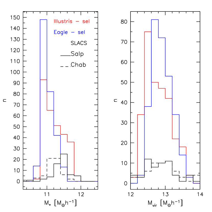
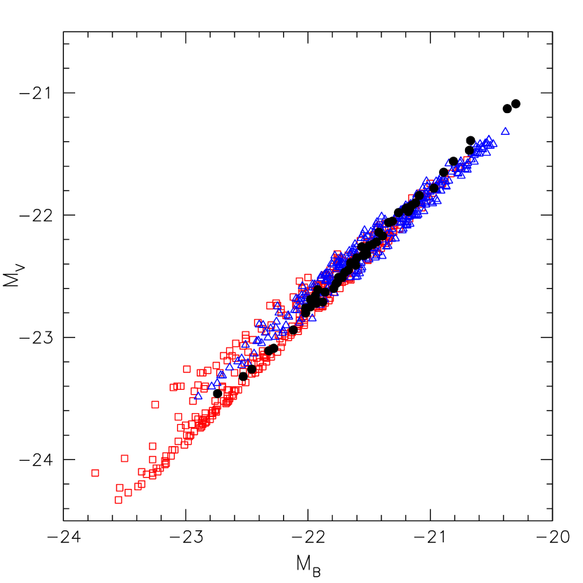
We investigate other similarities of the observed galaxies with the sample from simulations. Auger et al. (2010a) provide a relation to estimate the virial mass, based on a model that relates the virial and stellar masses (Moster et al., 2010), for various combinations of IMF (Chabrier, Salpeter and a Free model) and halo profile (NFW and two profiles from Blumenthal et al. 1986 and Gnedin et al. 2004 that take into account cooling and adiabatic contraction). These models define virial mass as the mass inside the radius enclosing the virial overdensity, as calculated from the spherical collapse model (Bryan & Norman, 1998). It is defined in the same way as in the simulations; we use the virial mass for the SLACS lenses calculated for a Salpeter IMF and profile from Gnedin et al. (2004). In Figure 6 we show the stellar and virial mass distributions of SLACS and of the selected sample of galaxies, finding a good agreement. Here we note that the virial mass of the two simulations peak at slightly different values, while stellar masses show a better agreement, bringing us back to the fact that Illustris has a higher stellar mass at fixed halo mass (Figure 7 - more details about the different composition of central haloes and subhaloes are presented in Appendix A). Nevertheless, it is possible to identify a good sample of analogues in both cases. In the bottom panel, we show the agreement between the data and the sample selected from simulations for what regards magnitudes, finding a good agreement. As discussed in Xu et al. (2016), who selected lens analogues in a similar way in the Illustris simulation, simulated early-type galaxies selected through velocity dispersion lie well on the fundamental plane.
6 Comparison with a real detection
In this section we quantify the probability of detecting substructures in SLACS-like lenses. Among the whole SLACS sample, 11 objects have been selected on a signal-to-noise basis and have been modelled searching for the presence of substructures (Vegetti et al., 2014). These are massive early-type lens galaxies, with an average velocity dispersion of and average Einstein radius . In this sample, only one lens has shown evidence of one substructure with a mass of (Vegetti et al., 2010). At the same time non-detections still carry important information and can be used to constrain the subhalo mass function. Our aim is to compare this rate of detections with a prediction from simulations: for this reason we will calculate the probability of detecting a substructure, with any mass larger than in a random sample of 11 haloes, chosen among the one we selected as SLACS analogues. We will then use the projected fraction of dark matter in subhaloes calculated from the analogues, in order to compare our estimates with that inferred from observations.
6.1 Detection probability
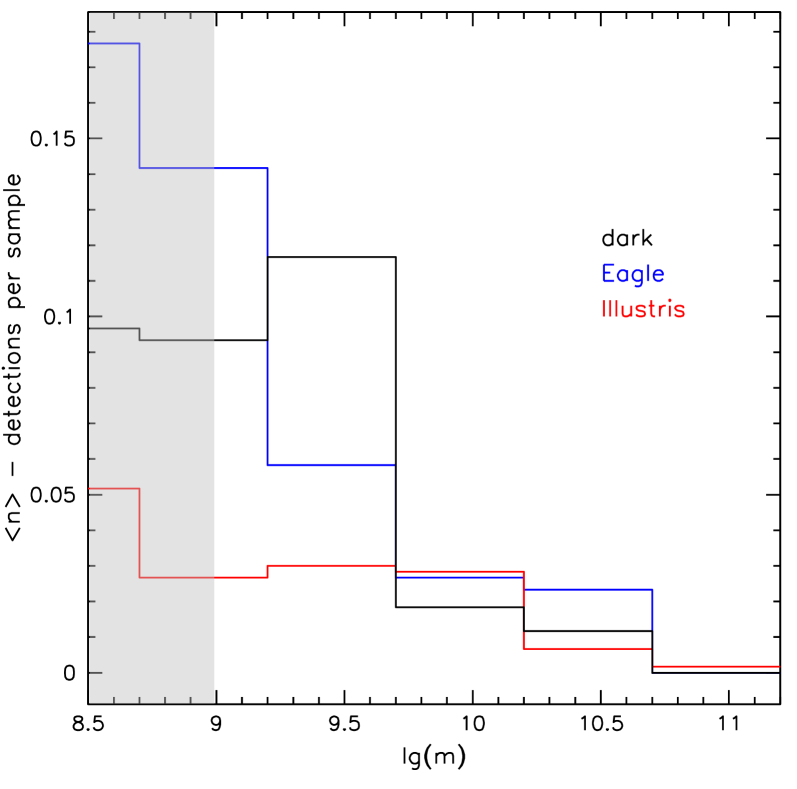
In order to determine the probability of one detection in a sample of 11 lenses, we extract 11 random haloes from our selection and project their substructures on the image of each lens. We repeat the procedure 600 times for each case (pure dark matter, EAGLE or Illustris hydro), to ensure a good statistic. We find that a substructure - with any mass larger than - is present in the sample of 11 lenses and in the area around the Einstein rings where it could affect the lensing signal in around 41, 37 and of the cases, respectively for dark-matter only, EAGLE and Illustris. Among these, probabilities are higher for low mass substructures, since - as seen in Figure 4 - the scaling between density and mass is of one order of magnitude for each decade in mass.
As detailed in Vegetti et al. (2014), counting how many substructures lie in the right region is not enough, because the possibility of detecting a substructure via its gravitational effect is not independent of its location: the effect of the substructure would be more evident for structured sources and in a location where a perturbation of the surface brightness could be stronger. In order to verify how many substructures can actually be detected, we make use of the sensitivity function maps created by Vegetti et al. (2014): these provide the minimum mass that could be detected for each pixel in the imaging of each of the 11 lenses. After projecting and counting the simulated subhaloes, we associate them with a pixelized grid with the same spacing of the sensitivity function and we compare the mass of the substructure with the sensitivity of the particular pixel it fells in: if the lowest detectable mass in that pixel is lower than the subhalo mass, then we consider it a detection, otherwise it is listed as non-detection. This leaves us with an overall probability of detecting one substructure with mass in one lens and nothing else in the others of 20, 19 and in the three cases, meaning that nearly of subhaloes are projected onto a pixel that is not sensitive enough to detect them. Figure 8 shows the average number of detected subhaloes with a mass larger than per sample of 11 objects, as a function of subhalo mass; probabilities in wider mass bins are summarized in Table 3. These results are compatible with the projected number counts of Figure 4, which are then further reduced by considering the sensitivity function. We point out that the sensitivity functions have been calculated using a detection as threshold: using weaker constraints may lead to higher detection probabilities from simulations. It should be noted that these conclusions are based exclusively on projected subhalo counts and we did not simulate the actual lensing effect of the subhaloes, which we plan to explore in a follow-up paper. Not only the number of subhaloes is different in different simulations, but also their structure, profile and concentration may change, leading to a different gravitational lensing effect. Understanding these differences and the contribution of the structures along the line-of-sight may allow to go beyond our results and effectively rule out some hydrodynamical models.
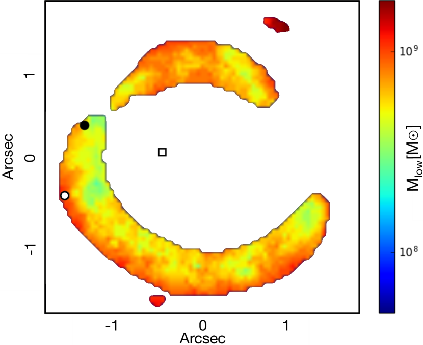
Figure 9 show three examples of substructures projected on the sensitivity function of the lens galaxy SDSSJ0946+1006, where there has been a real detection (Vegetti et al., 2010). The black point shows an example of detection: in the left panel the detected mass is - very similar to the real detection in this region, while in the right panel is . The white circle represent a non-detection case, where the mass of the substructure is lower than the minimum detectable mass, while the white square point shows a substructure that does not fall in the right region.
| percentage of detections using sensitivity functions | |||
|---|---|---|---|
| range [ | DMO | EAGLE | Illustris |
| 20 | 19 | 10 | |
| 18.5 | 17 | 8 | |
| 1.5 | 2 | 2 | |
6.2 Projected DM fraction
We now use our selection to calculate the mass fraction in subhaloes: we calculate the total projected dark matter mass in the area of the sensitivity functions by projecting the dark matter particles. For each of the selected haloes, we considered three independent projections for each of the 11 sensitivity functions. The resulting projected dark matter masses are generally consistent with those calculated for this sample of 11 SLACS lenses and on average of the order of . We then calculate the expected number density of subhaloes , as in Figure 4 for subhaloes with masses between and ; since this scales approximately of one order of magnitude for each decade in mass, we extrapolate the expected number of lower mass subhaloes between and that we do not resolve in the simulations. We then use the total projected dark matter mass and the number density of subhaloes in the sensitivity function areas, obtained multiplying the mean value for the total area. The mean densities in substructures in the range and the resulting mean mass fraction in substructures on the areas of the sensitivity functions are listed in Table 4. For the dark matter only case we are consistent with a value of compatible with Vegetti et al. (2014) - and thus consistent with the predictions from Xu et al. (2015). The mass fraction in substructure in the range is then lower for the simulations with baryons and especially for the Illustris simulation. These values, combined with the best fit slope of the subhalo mass function can be used to fully constrain the subhalo mass function and can be compared with those inferred from observations. Vegetti et al. (2014) found a mean substructure projected mass fraction of for a uniform prior on and for a gaussian prior with mean 1.9 and standard deviation 0.1. Thus, the values of (,) from the DMO and from the EAGLE hydro runs are compatible with their findings within the errors, both for the mass fraction and the slope . The results from the Illustris hydro run instead do not lie within the errors. If we use the double power-law fit to the subhalo mass function (from Table 1), we obtain slightly higher values of for the hydro runs; even in this case, the combination of (,) obtained from EAGLE is compatible with the observational results within the errors, while that obtained from Illustris is not, leaving our conclusions unchanged. We prefer the results obtained with a single power-law mass function for this comparison, in order to be consistent with the model used in the lensing analysis. We compare with this prediction and not with those of Vegetti et al. (2010) and Vegetti et al. (2012), since the first included only one lens and the second is based on a lens which is not part of the SLACS sample and has therefore a different selection criteria and a different mass and redshift.
| subhalo mass fraction | ||
|---|---|---|
| sim | ||
| DMO | 0.0044 0.0018 | |
| EAGLE | 0.00250.0012 | |
| Illustris | 0.00120.0004 | |
7 Summary
We have analysed the results of the two most recent simulations (EAGLE and Illustris), aiming to characterize the subhalo population in simulations with different baryonic physics models. We concentrate on haloes mass between and and redshift between 0.2 and 0.5, since we want to compare with observations of ETGs at these redshifts. Here we summarise our main results:
-
•
the presence of baryons modifies the abundance and structure of haloes, through processes such as adiabatic contractions, cooling, stellar and AGN feedback. As a consequence, the subhalo population is affected by the different abundance of haloes in the field that can be accreted by larger haloes and by a different dynamic and survival of substructure inside the main halo. Depending on the adopted physical model, the depletion in the low-mass end of the subhalo mass function changes: in the EAGLE hydro run, we find fewer subhaloes with a mass between and , while for the Illustris simulation this percentage can be as high as . A different effect is present also at higher subhalo masses (), where Illustris shows an excess of subhaloes in the hydro run, which is not present in EAGLE (Figure 1); this kind of differences need to be investigated more since they may be similar to those caused by warm dark matter models (Lovell et al., 2014; Li et al., 2016) at the low mass end.
- •
-
•
the projected number density of subhaloes is quite flat as a function of radius, as shown already by Xu et al. (2015) for a different mass range; the abundance of subhaloes that can be found in projection in the central regions of the halo decreases by about one order of magnitude for each decade in subhalo mass.
We conclude that baryonic physics has an important impact on the halo structure and on the subhalo population; this needs to be taken into account when we compare predictions from simulations to observational results. The reduction in the number of small subhaloes is a clear consequence of the presence of baryons and of stellar and AGN feedback. However, in order to distinguish this effect from others, such as that of warm dark matter models (Lovell et al., 2014; Li et al., 2016), we need to reach lower subhalo masses. We plan to investigate these differences with zoom-in high-resolution simulations in a follow-up paper.
The second part of this work focuses on the comparison with observational results, and in particular with the SLACS lenses. We searched for analogues in the simulations, considering ETGs which match the properties of the SLACS galaxies. We found a good number of these analogues at redshift between 0.2 and 0.5, selecting the galaxies by dynamical properties and velocity dispersion; we then verify that the selected galaxies lie in the right region of the plane and that the distribution of total stellar mass and virial mass are consistent with the observed ones. We use the selected galaxies to estimate subhalo detection probabilities with different physical models. For this, we extract random samples of 11 SLACS-like haloes from the simulations and project their substructure on the sensitivity functions of the real lenses, in order to estimate how many subhaloes could be detected. We conclude that:
-
•
1 detection with a mass in a sample of 11 lenses is not a certain event, and it has a probability of 20 (DMO), 19 (EAGLE) or 10 (Illustris);
-
•
many more observed lenses of ETG mass are needed to ensure a good number of detections and thus being able to fully constrain the subhalo mass function;
-
•
the dark matter fraction in subhaloes within the areas of the sensitivity functions, for the three models is (DMO, EAGLE, Illustris) = (0.0044,0.0025,0.0012). The values of (,) from the DMO and from the EAGLE hydro runs are both compatible with the findings of Vegetti et al. (2014) within the errors, while those from the Illustris are significantly lower
This clearly shows that substructure lensing not only allows to distinguish between different dark matter models, but also between feedback and galaxy formation models, provided that the contribution from the line-of-sight structures is well understood. This last aspect will be the main focus of a follow-up paper. Another scenario that needs to be addressed is that of different warm dark matter models, since it also causes a lack of low mass substructures; we plan to extend our findings to this and and to the combination between warm dark matter and baryons in a future work, using higher resolution simulations in order to reach lower masses.
8 Acknowledgments
We thank Dandan Xu, Simon White, Joop Schaye, Carlo Giocoli, Carlos Frenk, Rob Crain and Tom Theuns for useful discussions and comments. We thank Mark Lovell for providing some additional galaxy catalogues. We thank the EAGLE collaboration for granting us access to the data for this project. For part of this work, we used the DiRAC Data Centric system at Durham University, operated by the Institute for Computational Cosmology on behalf of the STFC DiRAC HPC Facility (www.dirac.ac.uk). This equipment was funded by BIS National E-infrastructure capital grant ST/K00042X/1, STFC capital grants ST/H008519/1 and ST/K00087X/1, STFC DiRAC Operations grant ST/K003267/1 and Durham University. DiRAC is part of the National E-Infrastructure. We thank the anonymous referee for his/her valuable comments that have helped us to improve the quality of the paper.
Appendix A Structure of subhaloes
We look at the structure of subhaloes and host haloes in the full hydrodynamical runs for the lens analogues. SUBFIND identifies the main “smooth” component of the FOF halo as the first and most massive subhalo, followed in the catalogue by all the smaller structures. In Figure 10 we distinguish the main halo and its subhaloes and study their baryonic content: we plot the average percentage of mass built up by stars and gas, respectively in orange and green. The right panel shows the composition of the central subhalo (i.e. the main halo) for the two simulations, at redshifts 0.2 and 1. The results from the two simulations present significant differences: in the EAGLE run, the main halo contains much more gas than in the Illustris and at the same time less gas is bound to the subhaloes. Moreover, we note again a higher stellar mass in Illustris galaxies, as in Figure 7. As shown in Schaye et al. (2015), the star formation is higher in the Illustris simulations for all masses and the feedback model induces a stronger AGN feedback, which expels almost all the gas from the halo with the purpose of quenching star formation - and is one of the known problems of the Illustris recipe. The effect of different feedback models on the baryon and gas fractions has been studied in Velliscig et al. (2014), who found an important depletion in the presence of an AGN. A selection of the simulated galaxies using observational constraints (as stellar mass, effective radius or magnitude) may thus be affected by the different composition of the central halo.
The left panels show the same for the subhaloes, binned by halo mass (different columns) and distance from the centre: the subhaloes which lie in the very centre of the halo - closer than - are represented by solid lines, while the others - between and - by dotted lines. First of all, we find - as in previous works - that the smallest subhaloes ( ) are almost completely dark and do not form stars. Moreover, subhaloes which lie near the centre lost the majority of their gas, so that stars build up to 40 of the total mass, while more distant satellites show fewer signs of stripping.
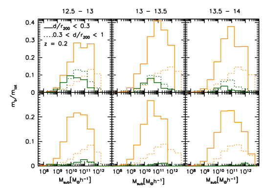

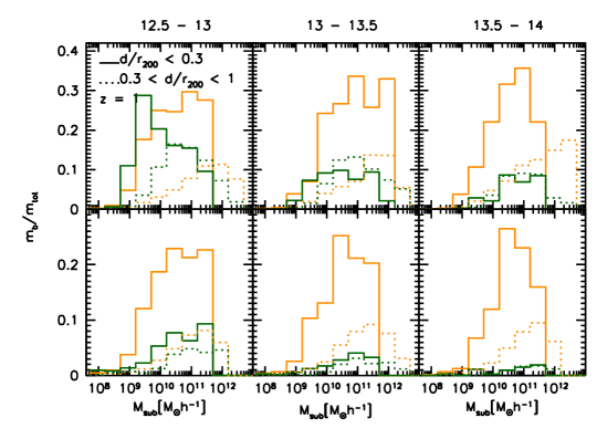
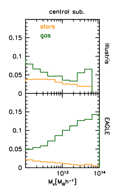
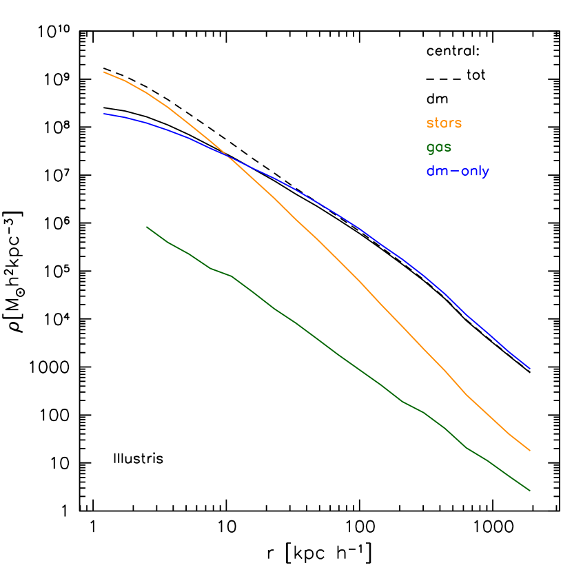
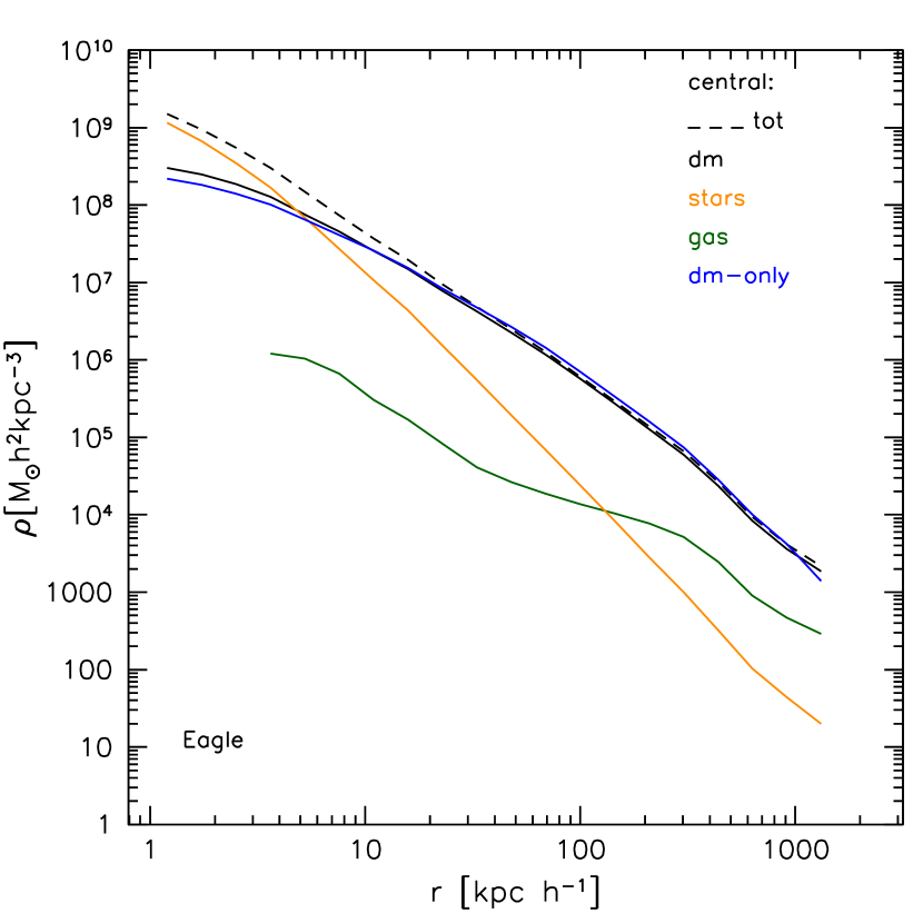
Figure 11 shows the mean radial density profiles of the central haloes. The mean density profile of the central is very similar in the two cases (Figure 11): stars and gas behave differently, but their contributions sum up to give a comparable total density profile.
We plan to analyse subhalo profiles and concentration in detail in a follow-up paper, using ray-tracing to model their influence on the lensing signal. Differences due to the baryonic physics implementation may arise and analysing possible systematic differences is important, as subhalo concentration plays a role in the possibility to observe them through gravitational lensing.
References
- Auger et al. (2009) Auger M. W., Treu T., Bolton A. S., Gavazzi R., Koopmans L. V. E., Marshall P. J., Bundy K., Moustakas L. A., 2009, ApJ, 705, 1099
- Auger et al. (2010b) Auger M. W., Treu T., Bolton A. S., Gavazzi R., Koopmans L. V. E., Marshall P. J., Moustakas L. A., Burles S., 2010b, ApJ, 724, 511
- Auger et al. (2010a) Auger M. W., Treu T., Gavazzi R., Bolton A. S., Koopmans L. V. E., Marshall P. J., 2010a, ApJ, 721, L163
- Bennett et al. (2013) Bennett C. L., Larson D., Weiland J. L., Jarosik N., Hinshaw G., Odegard N., Smith K. M., Hill R. S., et al. G., 2013, ApJS, 208, 20
- Blumenthal et al. (1986) Blumenthal G. R., Faber S. M., Flores R., Primack J. R., 1986, ApJ, 301, 27
- Bolton et al. (2006) Bolton A. S., Burles S., Koopmans L. V. E., Treu T., Moustakas L. A., 2006, ApJ, 638, 703
- Bryan & Norman (1998) Bryan G. L., Norman M. L., 1998, ApJ, 495, 80
- Crain et al. (2015) Crain R. A., Schaye J., Bower R. G., Furlong M., Schaller M., Theuns T., Dalla Vecchia C., Frenk C. S., McCarthy I. G., Helly J. C., Jenkins A., Rosas-Guevara Y. M., White S. D. M., Trayford J. W., 2015, MNRAS, 450, 1937
- Cui et al. (2012) Cui W., Borgani S., Dolag K., Murante G., Tornatore L., 2012, MNRAS, 423, 2279
- Cui et al. (2014) Cui W., Borgani S., Murante G., 2014, MNRAS, 441, 1769
- Dalal & Kochanek (2002) Dalal N., Kochanek C. S., 2002, ApJ, 572, 25
- Despali et al. (2016) Despali G., Giocoli C., Angulo R. E., Tormen G., Sheth R. K., Baso G., Moscardini L., 2016, MNRAS, 456, 2486
- Di Cintio et al. (2013) Di Cintio A., Knebe A., Libeskind N. I., Brook C., Yepes G., Gottlöber S., Hoffman Y., 2013, MNRAS, 431, 1220
- di Cintio et al. (2011) di Cintio A., Knebe A., Libeskind N. I., Yepes G., Gottlöber S., Hoffman Y., 2011, MNRAS, 417, L74
- Fiacconi et al. (2016) Fiacconi D., Madau P., Potter D., Stadel J., 2016, ApJ, 824, 144
- Garrison-Kimmel et al. (2014) Garrison-Kimmel S., Boylan-Kolchin M., Bullock J. S., Kirby E. N., 2014, MNRAS, 444, 222
- Giocoli et al. (2008) Giocoli C., Pieri L., Tormen G., 2008, MNRAS, 387, 689
- Giocoli et al. (2010a) Giocoli C., Tormen G., Sheth R. K., van den Bosch F. C., 2010a, MNRAS, 404, 502
- Gnedin et al. (2004) Gnedin O. Y., Kravtsov A. V., Klypin A. A., Nagai D., 2004, ApJ, 616, 16
- Grillo et al. (2009) Grillo C., Gobat R., Lombardi M., Rosati P., 2009, A&A, 501, 461
- Heitmann et al. (2008) Heitmann K., Lukić Z., Fasel P., Habib S., Warren M. S., White M., Ahrens J., Ankeny L., Armstrong R., O’Shea B., Ricker P. M., Springel V., Stadel J., Trac H., 2008, Computational Science and Discovery, 1, 015003
- Hezaveh et al. (2016) Hezaveh Y. D., Dalal N., Marrone D. P., Mao Y.-Y., Morningstar W., Wen D., Blandford R. D., Carlstrom J. E., Fassnacht C. D., Holder G. P., Kemball A., Marshall P. J., Murray N., Perreault Levasseur L., Vieira J. D., Wechsler R. H., 2016, ApJ, 823, 37
- Knebe et al. (2011) Knebe A., Knollmann S. R., Muldrew S. I., Pearce F. R., Aragon-Calvo M. A., Ascasibar Y., Behroozi P. S., Ceverino D., et al. 2011, MNRAS, 415, 2293
- Knebe et al. (2013) Knebe A., Pearce F. R., Lux H., Ascasibar Y., Behroozi P., Casado J., Moran C. C., Diemand J., et al. 2013, MNRAS, 435, 1618
- Li et al. (2016) Li R., Frenk C. S., Cole S., Gao L., Bose S., Hellwing W. A., 2016, MNRAS
- Lovell et al. (2012) Lovell M. R., Eke V., Frenk C. S., Gao L., Jenkins A., Theuns T., Wang J., White S. D. M., Boyarsky A., Ruchayskiy O., 2012, MNRAS, 420, 2318
- Lovell et al. (2014) Lovell M. R., Frenk C. S., Eke V. R., Jenkins A., Gao L., Theuns T., 2014, MNRAS, 439, 300
- Ludlow et al. (2012) Ludlow A. D., Navarro J. F., Li M., Angulo R. E., Boylan-Kolchin M., Bett P. E., 2012, MNRAS, 427, 1322
- McAlpine et al. (2016) McAlpine S., Helly J. C., Schaller M., Trayford e. a., 2016, Astronomy and Computing, 15, 72
- Moster et al. (2010) Moster B. P., Somerville R. S., Maulbetsch C., van den Bosch F. C., Macciò A. V., Naab T., Oser L., 2010, ApJ, 710, 903
- Muldrew et al. (2011) Muldrew S. I., Pearce F. R., Power C., 2011, MNRAS, 410, 2617
- Nelson et al. (2015) Nelson D., Pillepich A., Genel S., Vogelsberger M., Springel V., et al. T., 2015, Astronomy and Computing, 13, 12
- Neto et al. (2007) Neto A. F., Gao L., Bett P., Cole S., Navarro J. F., Frenk C. S., White S. D. M., Springel V., Jenkins A., 2007, MNRAS, 381, 1450
- Nierenberg et al. (2014) Nierenberg A. M., Treu T., Wright S. A., Fassnacht C. D., Auger M. W., 2014, MNRAS, 442, 2434
- Onions et al. (2012) Onions J., Knebe A., Pearce F. R., Muldrew S. I., Lux H., Knollmann S. R., Ascasibar Y., Behroozi P., Elahi P., Han J., Maciejewski M., Merchán M. E., Neyrinck M., Ruiz A. N., Sgró M. A., Springel V., Tweed D., 2012, MNRAS, 423, 1200
- Planck Collaboration et al. (2014) Planck Collaboration Ade P. A. R., Aghanim N., Alves M. I. R., Armitage-Caplan C., Arnaud M., Ashdown M., Atrio-Barandela F., Aumont J., Aussel H., et al. 2014, A&A, 571, A1
- Sawala et al. (2013) Sawala T., Frenk C. S., Crain R. A., Jenkins A., Schaye J., Theuns T., Zavala J., 2013, MNRAS, 431, 1366
- Sawala et al. (2015) Sawala T., Frenk C. S., Fattahi A., Navarro J. F., Bower R. G., Crain R. A., Dalla Vecchia C., Furlong M., Jenkins A., McCarthy I. G., Qu Y., Schaller M., Schaye J., Theuns T., 2015, MNRAS, 448, 2941
- Sawala et al. (2017) Sawala T., Pihajoki P., Johansson P. H., Frenk C. S., Navarro J. F., Oman K. A., White S. D. M., 2017, MNRAS, 467, 4383
- Schaller et al. (2015) Schaller M., Frenk C. S., Bower R. G., Theuns T., Jenkins A., Schaye J., Crain R. A., Furlong M., Dalla Vecchia C., McCarthy I. G., 2015, MNRAS, 451, 1247
- Schaye et al. (2015) Schaye J., Crain R. A., Bower R. G., Furlong M., Schaller M., Theuns T., Dalla Vecchia C., Frenk C. S. e. a., 2015, MNRAS, 446, 521
- Sheth & Tormen (1999) Sheth R. K., Tormen G., 1999, MNRAS, 308, 119
- Snyder et al. (2015) Snyder G. F., Torrey P., Lotz J. M., Genel S., McBride C. K., Vogelsberger M., Pillepich A., Nelson D., Sales L. V., Sijacki D., Hernquist L., Springel V., 2015, MNRAS, 454, 1886
- Springel (2010) Springel V., 2010, MNRAS, 401, 791
- Springel et al. (2008) Springel V., Wang J., Vogelsberger M., Ludlow A., Jenkins A., Helmi A., Navarro J. F., Frenk C. S., White S. D. M., 2008, MNRAS, 391, 1685
- Springel et al. (2008) Springel V., White S. D. M., Frenk C. S., Navarro J. F., Jenkins A., Vogelsberger M., Wang J., Ludlow A., Helmi A., 2008, Nature, 456, 73
- Springel et al. (2001b) Springel V., White S. D. M., Tormen G., Kauffmann G., 2001b, MNRAS, 328, 726
- Teklu et al. (2015) Teklu A. F., Remus R.-S., Dolag K., Beck A. M., Burkert A., Schmidt A. S., Schulze F., Steinborn L. K., 2015, ApJ, 812, 29
- Vegetti & Koopmans (2009) Vegetti S., Koopmans L. V. E., 2009, MNRAS, 392, 945
- Vegetti et al. (2014) Vegetti S., Koopmans L. V. E., Auger M. W., Treu T., Bolton A. S., 2014, MNRAS, 442, 2017
- Vegetti et al. (2010) Vegetti S., Koopmans L. V. E., Bolton A., Treu T., Gavazzi R., 2010, MNRAS, 408, 1969
- Vegetti et al. (2012) Vegetti S., Lagattuta D. J., McKean J. P., Auger M. W., Fassnacht C. D., Koopmans 2012, Nature, 481, 341
- Velliscig et al. (2014) Velliscig M., van Daalen M. P., Schaye J., McCarthy I. G., Cacciato M., Le Brun A. M. C., Dalla Vecchia C., 2014, MNRAS, 442, 2641
- Vogelsberger et al. (2014) Vogelsberger M., Genel S., Springel V., Torrey P., Sijacki D., Xu D., Snyder G., Nelson D., Hernquist L., 2014, MNRAS, 444, 1518
- Wetzel et al. (2016) Wetzel A. R., Hopkins P. F., Kim J.-h., Faucher-Giguère C.-A., Kereš D., Quataert E., 2016, ApJ, 827, L23
- Xu et al. (2015) Xu D., Sluse D., Gao L., Wang J., Frenk C., Mao S., Schneider P., Springel V., 2015, MNRAS, 447, 3189
- Xu et al. (2016) Xu D., Springel V., Sluse D., Schneider P., Sonnenfeld A., Nelson D., Vogelsberger M., Hernquist L., 2016, ArXiv:1610.07605
- Zhu et al. (2016) Zhu Q., Marinacci F., Maji M., Li Y., Springel V., Hernquist L., 2016, MNRAS, 458, 1559