Exact critical exponents for the antiferromagnetic quantum critical metal in two dimensions

Abstract

Unconventional metallic states which do not support well defined single-particle excitations can arise near quantum phase transitions as strong quantum fluctuations of incipient order parameters prevent electrons from forming coherent quasiparticles. Although antiferromagnetic phase transitions occur commonly in correlated metals, understanding the nature of the strange metal realized at the critical point in layered systems has been hampered by a lack of reliable theoretical methods that take into account strong quantum fluctuations. We present a non-perturbative solution to the low-energy theory for the antiferromagnetic quantum critical metal in two spatial dimensions. Being a strongly coupled theory, it can still be solved reliably in the low-energy limit as quantum fluctuations are organized by a new control parameter that emerges dynamically. We predict the exact critical exponents that govern the universal scaling of physical observables at low temperatures.

I Introduction

One of the cornerstones of condensed matter physics is Landau Fermi liquid theory, according to which quantum many-body states of interacting electrons are described by largely independent quasiparticles in metalsLandau (1957). In Fermi liquids, the spectral weight of an electron is sharply peaked at a well defined energy due to the quasiparticles with long lifetimes. On the other hand, exotic metallic states beyond the quasiparticle paradigm can arise near quantum critical points, where quantum fluctuations of collective modes driven by the uncertainty principle preempt the existence of well defined single-particle excitationsHertz (1976); Millis (1993); Löhneysen et al. (2007); Stewart (2001). In the absence of quasiparticles, many-body states become qualitatively different from a direct product of single particle wavefunctions. Due to strong fluctuations near the Fermi surface, the delta function peak of the electron spectral function is smeared out, leaving a weaker singularity behind. The resulting non-Fermi liquids exhibit unconventional power-law dependences of physical observables on temperature and probe energySenthil (2008). A primary theoretical goal is to understand the universal scaling behavior of the observables based on low-energy effective theories that replace Fermi liquid theory for the unconventional metals Holstein et al. (1973); Reizer (1989); Altshuler et al. (1994); Kim et al. (1994); Lee (1989); Polchinski (1994); Lee and Nagaosa (1992); Nayak and Wilczek (1994); Lee (2009); Metlitski and Sachdev (2010a); Mross et al. (2010); Jiang et al. (2013); Dalidovich and Lee (2013); Sur and Lee (2014); Holder and Metzner (2015).

Antiferromagnetic (AF) quantum phase transitions arise in a wide range of layered compounds Helm et al. (2010); Hashimoto et al. (2012); Park et al. (2006). Despite the recent progress made in field theoretic and numerical approaches to the AF quantum critical metal Abanov and Chubukov (2000); Abanov et al. (2003); Abanov and Chubukov (2004); Metlitski and Sachdev (2010b); Abrahams and Wolfle (2012); Sur and Lee (2015); Maier and Strack (2016); Berg et al. (2012); Schattner et al. (2015), a full understanding of the non-Fermi liquid realized at the critical point has been elusive so far. In two dimensions, strong quantum fluctuations and abundant low-energy particle-hole excitations render perturbative theories inapplicable. What is needed is a non-perturbative approach which takes into account strong quantum fluctuations in a controlled waySur and Lee (2014).

In this article, we present a non-perturbative field theoretic study of the AF quantum critical metal in two dimensions. Although the theory becomes strongly coupled at low energies, we demonstrate that a small parameter which differs from the conventional coupling emerges dynamically. This allows us to solve the strongly interacting theory reliably. We predict the exact critical exponents that govern the scaling of dynamical and thermodynamic observables.

II Low-energy theory and interaction-driven scaling

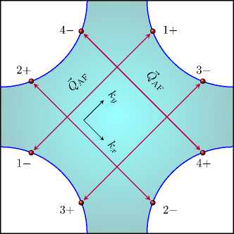
Figure 1: A Fermi surface with the four-fold rotational symmetry. The (red) dots represent the hot spots connected by the AF wavevector $\vec{Q}_{AF}$.

The relevant low-energy degrees of freedom at the metallic AF critical point are the AF collective mode and electrons near the hot spots, a set of points on the Fermi surface connected by the AF wavevector. In the presence of the four-fold rotational symmetry and the reflection symmetry in two spatial dimensions, there are generically eight hot spots, as is shown in Figure 1. Following Ref. Sur and Lee (2015), we write the action as

$$\mathcal{S} =\sum_{n=1}^{4}\sum_{\sigma=\uparrow,\downarrow}\int dk~{}\bar{\Psi}_{n,\sigma}(k)\Bigl{[}i\gamma_{0}k_{0}+i\gamma_{1}\varepsilon_{n}(\vec{k})\Bigr{]}\Psi_{n,\sigma}(k)$$

$$+\frac{1}{4}\int dq~{}\Bigl{[}q_{0}^{2}+c_{0}^{2}|\vec{q}|^{2}\Bigr{]}\mbox{Tr}\left[{\Phi(-q)~{}\Phi(q)}\right]$$

$$+ig\sum_{n=1}^{4}\sum_{\sigma,\sigma^{\prime}}\int dkdq~{}\Bigl{[}\bar{\Psi}_{\bar{n},\sigma}(k+q)\Phi_{\sigma,\sigma^{\prime}}(q)\gamma_{1}\Psi_{n,\sigma^{\prime}}(k)\Bigr{]}$$

$$+u\int dk_{1}dk_{2}dq~{}\mbox{Tr}\left[{\Phi(k_{1}+q)\Phi(k_{2}-q)}\right]\mbox{Tr}\left[{\Phi(-k_{1})\Phi(-k_{2})}\right].$$ (1)

Here $k=(k_{0},\vec{k})$ denotes Matsubara frequency and two-dimensional momentum $\vec{k}=(k_{x},k_{y})$ with $dk\equiv\frac{d^{3}k}{(2\pi)^{3}}$. The four spinors are defined by $\Psi_{1,\sigma}=(\psi^{(+)}_{1,\sigma},\psi^{(+)}_{3,\sigma})^{T}$, $\Psi_{2,\sigma}=(\psi^{(+)}_{2,\sigma},\psi^{(+)}_{4,\sigma})^{T}$, $\Psi_{3,\sigma}=(\psi^{(-)}_{1,\sigma},-\psi^{(-)}_{3,\sigma})^{T}$ and $\Psi_{4,\sigma}=(\psi^{(-)}_{2,\sigma},-\psi^{(-)}_{4,\sigma})^{T}$, where $\psi^{(m)}_{n,\sigma}$’s are electron fields with spin $\sigma=\uparrow,\downarrow$ near the hot spots labeled by $n=1,2,3,4$, $m=\pm$. $\bar{\Psi}_{n,\sigma}=\Psi^{\dagger}_{n,\sigma}\gamma_{0}$, where $\gamma_{0}=\sigma_{y},\gamma_{1}=\sigma_{x}$ are $2\times 2$ gamma matrices for the spinors. The energy dispersions of the electrons near the hot spots are written as $\varepsilon_{1}(\vec{k})=vk_{x}+k_{y}$, $\varepsilon_{2}(\vec{k})=-k_{x}+vk_{y}$, $\varepsilon_{3}(\vec{k})=vk_{x}-k_{y}$ and $\varepsilon_{4}(\vec{k})=k_{x}+vk_{y}$, where $\vec{k}$ represents the deviation of momentum away from each hot spot. The commensurate AF wavevector ${\vec{Q}}_{AF}$ is chosen to be parallel to the $x$ and $y$ directions modulo reciprocal lattice vectors. The component of the Fermi velocity parallel to ${\vec{Q}}_{AF}$ at each hot spot is set to have unit magnitude. $v$ measures the component of the Fermi velocity perpendicular to ${\vec{Q}}_{AF}$. $\Phi(q)=\sum_{a=1}^{3}\phi^{a}(q)\tau^{a}$ is a $2\times 2$ matrix boson field that represents the fluctuating AF order parameter, where the $\tau^{a}$’s are the generators of the $SU(2)$ spin. $c_{0}$ is the velocity of the AF collective mode. $g$ is the coupling between the collective mode and the electrons near the hot spots. $\bar{n}$ represents the hot spot connected to $n$ via $\vec{Q}_{AF}$ : $\bar{1}=3,\bar{2}=4,\bar{3}=1,\bar{4}=2$. $u$ is the quartic coupling between the collective modes.

In two dimensions, the conventional perturbative expansion becomes unreliable as the couplings grow at low energies. Since the interaction plays a dominant role, we need to include the interaction up front rather than treating it as a perturbation to the kinetic energy. Therefore, we start with an interaction-driven scalingSur and Lee (2014) in which the fermion-boson coupling is deemed marginal. Under such a scaling, one cannot keep all the kinetic terms as marginal operators. Here we choose a scaling that keeps the fermion kinetic term marginal at the expense of making the boson kinetic term irrelevant. This choice will be justified through explicit calculations. It reflects the fact that the dynamics of the boson is dominated by particle-hole excitations near the Fermi surface in the low-energy limit, unless the number of bosons per fermion is infiniteFitzpatrick et al. (2013). The marginality of the fermion kinetic term and the fermion-boson coupling uniquely fixes the dimensions of momentum and the fields under the interaction-driven tree-level scaling,

$$[k_{0}]=[k_{x}]=[k_{y}]=1,$$

$$[\psi(k)]=[\phi(k)]=-2.$$ (2)

Under this scaling, the electron keeps the classical scaling dimension, while the boson has an $O(1)$ anomalous dimension compared to the Gaussian scaling. At this point, Eq. (2) is merely an Ansatz. The real test is to show that these exponents are actually exact, which is the main goal of this paper.

Under Eq. (2), the entire boson kinetic term and the quartic coupling are irrelevant. The minimal action which includes only marginal terms is written as

$$\mathcal{S} =\sum_{n=1}^{4}\sum_{\sigma=\uparrow,\downarrow}\int dk~{}\bar{\Psi}_{n,\sigma}(k)\Bigl{[}i\gamma_{0}k_{0}+i\gamma_{1}\varepsilon_{n}(\vec{k})\Bigr{]}\Psi_{n,\sigma}(k)$$

$$+i\sqrt{\frac{\pi v}{2}}\sum_{n=1}^{4}\sum_{\sigma,\sigma^{\prime}}\int dkdq~{}\Bigl{[}\bar{\Psi}_{\bar{n},\sigma}(k+q)\Phi_{\sigma,\sigma^{\prime}}(q)\gamma_{1}\Psi_{n,\sigma^{\prime}}(k)\Bigr{]}.$$ (3)

Here, the fermion-boson coupling is set to be proportional to $\sqrt{v}$ by rescaling the boson field. The Yukawa coupling is replaced with $\sqrt{v}$ because the interaction is screened such that $g^{2}$ becomes $O(v)$ in the low-energy limitSur and Lee (2015). Although $g$ and $v$ can be independently tuned in the microscopic theory, they rapidly flow to a universal line defined by $g^{2}\sim v$ at low energiesLunts et al. (2017). Eq. (3) should be understood as the minimal theory that captures the universal physics at low energies, where the dynamics of the collective mode is dominated by particle-hole excitations rather than the bare kinetic term, and $v$ is the only dimensionless parameter. In the small $v$ limit, $g$ also vanishes because a nested Fermi surface provides a large phase space for low-energy particle-hole excitations with momentum $\vec{Q}_{AF}$ that screen the interaction. Even when $g,v$ are small, this is a strongly interacting theory because $g^{2}/v\sim 1$ is the expansion parameter in the conventional perturbative series. With $g^{2}/v\sim 1$, the leading boson kinetic term which is generated from particle-hole excitations is $O(1)$, as will be seen later.

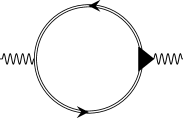
Figure 2: The exact boson self-energy. The double line is the fully dressed fermion propagator. The triangle represents the fully dressed vertex.

III Self-consistent solution

Naively the theory is singular due to the absence of a boson kinetic term. However, particle-hole excitations generate a self-energy which provides non-trivial dynamics for the collective mode. The Schwinger-Dyson equation for the boson propagator (shown in Figure 2) reads

$$D(q)^{-1} = m_{CT}-\pi v\sum_{n}\int dk~{}\mbox{Tr}\left[\gamma_{1}G_{\bar{n}}(k+q)\Gamma(k,q)G_{n}(k)\right].$$ (4)

Here $D(k)$, $G(k)$ and $\Gamma(k,q)$ represent the fully dressed propagators of the boson and the fermion, and the vertex function, respectively. $m_{CT}$ is a mass counter term that is added to tune the renormalized mass to zero. The trace in Eq. (4) is over the spinor indices. It is difficult to solve the full self-consistent equation because $G(k)$ and $\Gamma(k,q)$ depend on the unknown $D(q)$. One may use $v$ as a small parameter to solve the equation. The one-loop analysis shows that $v$ flows to zero due to emergent nesting of the Fermi surface near the hot spotsAbanov and Chubukov (2000); Abanov et al. (2003); Metlitski and Sachdev (2010b); Maier and Strack (2016). This has been also confirmed in the $\epsilon$ expansion based on the dimensional regularization schemeSur and Lee (2015); Lunts et al. (2017). Of course, the perturbative result valid close to three dimensions does not necessarily extend to two dimensions. Nonetheless, we show that this is indeed the case. Here we proceed with the following steps:

1. we solve the Schwinger-Dyson equation for the boson propagator in the small $v$ limit,

2. we show that $v$ flows to zero at low energies by using the boson propagator obtained under the assumption of $v\ll 1$.

We emphasize that the expansion in $v$ is different from the conventional perturbative expansion in coupling. Rather it involves a non-perturbative summation over an infinite series of diagrams as will be shown in the following.

We discuss step 1) first. In the small $v$ limit, the solution to the Schwinger-Dyson equation is

$$D(q)^{-1}=|q_{0}|+c(v)\Big{[}|q_{x}|+|q_{y}|\Big{]},$$ (5)

where the ‘velocity’ of the strongly damped collective mode is given by

$$c(v)=\frac{1}{4}\sqrt{v\log(1/v)}.$$ (6)

Solving the Schwinger-Dyson equation consists of two parts. First, we assume Eq. (5) with a hierarchy of the velocities $v\ll c(v)\ll 1$ as an Ansatz to show that only the one-loop vertex correction is important in Eq. (4). Then we show that Eqs. (5) and (6) actually satisfy Eq. (4) with the one-loop dressed vertex.

We begin by estimating the magnitude of general diagrams, assuming that the fully dressed boson propagator is given by Eq. (5) with Eq. (6) in the small $v$ limit. In general, the integrations over loop momenta diverge in the small $v$ limit as fermions and bosons lose their dispersion in some directions. In each fermion loop, the component of the internal momentum tangential to the Fermi surface is unbounded in the small $v$ limit due to nesting. For a small but nonzero $v$, the divergence is cut off at a scale proportional to $1/v$, and each fermion loop contributes a factor of $1/v$. Each of the remaining loops necessarily has at least one boson propagator. For those loops, the momentum along the Fermi surface is cut off by the energy of the boson which provides a lower cut-off momentum proportional to $1/c$ for $c\gg v$. Therefore, the magnitude of a general $L$-loop diagram with $V$ vertices, $L_{f}$ fermion loops and $E$ external legs is at most

$$I\sim v^{V/2-L_{f}}c^{-(L-L_{f})}\sim v^{\frac{1}{2}(E-2)}\left(\frac{v}{c}\right)^{(L-L_{f})},$$ (7)

where $V=2L+E-2$ is used. Higher-loop diagrams are systematically suppressed with increasing $(L-L_{f})$ provided $v\ll c$. This is analogous to the situation where a ratio between velocities is used as a control parameter in a Dirac semi-metalHuh and Sachdev (2008) . If Eq. (6) holds, the upper bound becomes $I\sim v^{\frac{1}{2}(E-2)+\frac{1}{2}(L-L_{f})}$ up to a logarithmic correction. It is noted that Eq. (7) is only an upper bound because some loop integrals which involve un-nested fermions remain finite even in the small $v$ limit. Some diagrams can also be smaller than the upper bound because their dependences on external momentum are suppressed in the small $v$ and $c$ limit. A systematic proof of Eq. (7) is available in Appendix A.

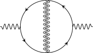
Figure 3: The leading order diagrams for the boson self-energy in the small $v$ limit. Solid lines are the bare fermion propagators. The wiggly double line represents the boson propagator consistently dressed with the self-energy in (a) and (b). The dressed boson propagator includes an infinite series of nested self-energies with a fractal structure.

For $v\ll c$, the leading order contribution for the boson self-energy ($E=2$) is generated from Figure 3, which is the only diagram that satisfies $L=L_{f}$. All other diagrams are sub-leading in $v$. However, this is not enough because the one-loop diagram gives $D(q)^{-1}=|q_{0}|$, which is independent of spatial momentum. One has to include the next order diagram (Figure 3) which generates a dispersion. Therefore, Eq. (4) is reduced to

$$D(q)^{-1}=m_{CT}^{{}^{\prime}}+|q_{0}|$$

$$-\frac{\pi^{2}v^{2}}{2}\sum_{n}\int dp~{}dk~{}\mbox{Tr}\left[{\gamma_{1}G_{n}^{(0)}(k+p)\gamma_{1}G_{\bar{n}}^{(0)}(p+q+k)\gamma_{1}G_{n}^{(0)}(q+k)\gamma_{1}G_{\bar{n}}^{(0)}(k)}\right]D(p).$$

(8)

Here $m_{CT}^{{}^{\prime}}$ is a two-loop mass counter term. We can use the free fermion propagator $G^{(0)}_{n}$ because the fermion self-energy correction is sub-leading in $v$. An explicit calculation of Eq. (8) confirms that the self-consistent boson propagator takes the form of Eq. (5). The boson velocity satisfies the self-consistent equation $c=\frac{v}{8c}\log(c/v)$, which is solved by Eq. (6) in the small $v$ limit. $c$ is much larger than $v$ in the small $v$ limit because of the enhancement factor $1/c$ in the two-loop diagram : the collective mode speeds up itself through enhanced quantum fluctuations if it gets too slow. We note that the anti-screening nature of the vertex correction associated with the non-Abelian $SU(2)$ vertex, $\sum_{a=1}^{3}\tau^{a}\tau^{b}\tau^{a}=-\tau^{b}$, is crucial to generate the right sign for the boson kinetic termSur and Lee (2016). This does not hold for Ising-like or XY-like spin fluctuationsVarma (2015). The details on the computation of Eq. (8) are available in Appendix B. It is noted that Eq. (8) constitutes a non-perturbative sum over an infinite series of diagrams beyond the random phase approximation (RPA). The dynamics of the boson generated from the fermionic sector dominates at low energies. This justifies the choice to drop the bare kinetic term in Eq. (3).

So far, we have assumed that $v$ is small to obtain the self-consistent dynamics of the AF collective mode. Now we turn to step 2) and show that $v$ indeed flows to zero in the low-energy limit. According to Eq. (7), the leading quantum corrections to the local action in Eq. (3) are the one-loop diagrams for the fermion self-energy and the vertex function. However, the momentum-dependent one-loop fermion self-energy happens to be smaller than what is expected from Eq. (7) by an additional power of $c\sim\sqrt{v}$. This is because the dependence on the external momentum is suppressed in the small $c$ limit for the one-loop self-energy. As a result, we include the fermion self-energy up to two loops in order to capture all quantum corrections to the leading order in $v$. All other higher-loop diagrams are negligible in the small $v$ limit. The self-energy and vertex correction are logarithmically divergent in a UV cut-off. Counter terms are added such that the renormalized quantum effective action becomes independent of the UV cut-off. The full details on the computation of the counter terms and the beta function can be found in Appendix C. The bare action that includes the counter terms is obtained to be

$$\mathcal{S}_{B} =\sum_{n=1}^{4}\sum_{\sigma=\uparrow,\downarrow}\int d^{3}k~{}\bar{\Psi}_{n,\sigma}(k)\Bigl{[}iZ_{1}\gamma_{0}k_{0}+i\gamma_{1}\varepsilon_{n}^{B}(\vec{k})\Bigr{]}\Psi_{n,\sigma}(k)$$

$$+iZ_{6}\sqrt{\frac{\pi v}{2}}\sum_{n=1}^{4}\sum_{\sigma,\sigma^{\prime}}\int d^{3}kd^{3}q~{}\Bigl{[}\bar{\Psi}_{\bar{n},\sigma}(k+q)\Phi_{\sigma,\sigma^{\prime}}(q)\gamma_{1}\Psi_{n,\sigma^{\prime}}(k)\Bigr{]},$$ (9)

where $\varepsilon_{1}^{B}(\vec{k})=Z_{2}vk_{x}+Z_{3}k_{y}$, $\varepsilon_{2}^{B}(\vec{k})=-Z_{3}k_{x}+Z_{2}vk_{y}$, $\varepsilon_{3}^{B}(\vec{k})=Z_{2}vk_{x}-Z_{3}k_{y}$ and $\varepsilon_{4}^{B}(\vec{k})=Z_{3}k_{x}+Z_{2}vk_{y}$ with $Z_{1}=1-\frac{3}{4\pi}\frac{v}{c(v)}\log\left(\frac{\Lambda}{\mu}\right)$, $Z_{2}=1+\frac{15}{4\pi^{2}}v\,\log\left(\frac{1}{c(v)}\right)\,\log\left(\frac{\Lambda}{\mu}\right)$, $Z_{3}=1-\frac{9}{4\pi^{2}}v\,\log\left(\frac{1}{c(v)}\right)\,\log\left(\frac{\Lambda}{\mu}\right)$ and $Z_{6}=1-\frac{1}{4\pi}\frac{v}{c(v)}\log\left(\frac{c(v)}{v}\right)\log\left(\frac{\Lambda}{\mu}\right)$. Here $\Lambda$ is a UV cut-off above which non-linear terms in the fermionic dispersion become important. $\mu$ is the scale at which the physical propagators and vertex function are expressed in terms of $v$ through the renormalization conditions, $\frac{-i}{2}\left.\frac{\partial}{\partial k_{0}}\mbox{Tr}\left[{\gamma_{0}G_{1}(k)^{-1}}\right]\right|_{k=(\mu,0,0)}=1+F_{1}(v)$, $\frac{-i}{2}\left.\frac{\partial}{\partial k_{x}}\mbox{Tr}\left[{\gamma_{1}G_{1}(k)^{-1}}\right]\right|_{k=(0,\mu,0)}=v\left(1+F_{2}(v)\right)$, $\frac{-i}{2}\left.\frac{\partial}{\partial k_{y}}\mbox{Tr}\left[{\gamma_{1}G_{1}(k)^{-1}}\right]\right|_{k=(0,0,\mu)}=1+F_{3}(v)$, $\frac{1}{2}\left.\mbox{Tr}\left[{\gamma_{1}\Gamma(k,q)}\right]\right|_{q=0,k=(\mu,0,0)}=1+F_{4}(v)$, where the $F_{i}(v)$’s are UV-finite functions of $v$, which vanish in the small $v$ limit. The specific form of $F_{i}(v)$ is unimportant, and they can be changed by adding finite counter terms in $Z_{i}$. $G_{n}(k)$ with $n=2,3,4$ are fixed from $G_{1}(k)$ by the four-fold rotational symmetry. The bare and renormalized variables are related to each other through $k_{B,x}=k_{x}$, $k_{B,y}=k_{y}$, $k_{B,0}=\frac{Z_{1}}{Z_{3}}k_{0}$, $v_{B}=\frac{Z_{2}}{Z_{3}}v$, $\Psi_{B}(k_{B})=\frac{Z_{3}}{Z_{1}^{\frac{1}{2}}}\Psi(k)$, $\Phi_{B}(k_{B})=\frac{Z_{3}^{\frac{1}{2}}Z_{6}}{Z_{1}Z_{2}^{\frac{1}{2}}}\,\Phi(k)$. By requiring that the bare quantities are independent of $\mu$, we obtain the beta function $\beta_{v}\equiv\frac{dv}{d\log\mu}$, which dictates the dependence of the renormalized velocity on the scale,

$$\beta_{v}=\frac{6}{\pi^{2}}\,v^{2}\log\left(\frac{1}{c(v)}\right).$$ (10)

As a function of the energy scale $\mu$, $v$ is renormalized according to

$$\frac{dv}{d\log\mu}=\frac{6}{\pi^{2}}\,v^{2}\log\left(\frac{1}{c(v)}\right).$$ (11)

If $v$ is initially small, Eq. (11) is reliable. It predicts that $v$ becomes even smaller and flows to zero as

$$v=\frac{\pi^{2}}{3}\left(\log\frac{1}{\mu}~{}\log\log\frac{1}{\mu}\right)^{-1}$$ (12)

in the small $\mu$ limit. The way $v$ flows to zero in the low-energy limit does not depend on the initial value of $v$. This completes the cycle of self-consistency. Eq. (5) obtained in the small $v$ limit becomes asymptotically exact in the low-energy limit within a nonzero basin of attraction in the space of $v$ whose fixed point is $v=0$. The dynamical critical exponent and the anomalous dimensions are given by

$$z = 1+\frac{3}{4\pi}\frac{v}{c(v)},$$

$$\eta_{\phi} = \frac{1}{4\pi}\frac{v}{c(v)}\log\left(\frac{c(v)}{v}\right),$$

$$\eta_{\psi} = -\frac{3}{8\pi}\frac{v}{c(v)}$$ (13)

to the leading order in $v$. Here $z$ sets the dimension of frequency relative to momentum. $\eta_{\phi}$, $\eta_{\psi}$ are the corrections to the interaction-driven tree-level scaling dimensions of the boson and fermion, respectively. The critical exponents are controlled by $w\equiv v/c(v)$, which flows to zero as $w=\frac{4\pi}{\sqrt{3}}\left(\log^{1/2}\frac{1}{\mu}~{}\log\log\frac{1}{\mu}\right)^{-1}$ in the low-energy limit. This confirms that the scaling dimensions in Eq. (2) become asymptotically exact in the low-energy limit. This is compatible with the fact that an inclusion of higher-loop corrections in the $\epsilon$-expansion reproduces $z=1$, irrespective of $\epsilon$Lunts et al. (2017).

IV Physical observables

Although $z-1$, $\eta_{\psi}$ and $\eta_{\phi}$ vanish in the low-energy limit, the sub-logarithmic decay of $w$ with energy introduces corrections to the correlation functions at intermediate energy scales, which are weaker than power-law but stronger than logarithmic correctionsVarma et al. (1989). The retarded Green’s function for the hot spot $1+$ takes the form,

$$G^{R}_{1+}(\omega,\vec{k})=\frac{1}{F_{\psi}(\omega)\left[\omega~{}F_{z}(\omega)\left(1+i\frac{\sqrt{3}\pi}{2}\frac{1}{\sqrt{\log\frac{1}{\omega}}~{}\log\log\frac{1}{\omega}}\right)-\left(\frac{\pi^{2}}{3}\frac{k_{x}}{\log\frac{1}{\omega}~{}\log\log\frac{1}{\omega}}+k_{y}\right)\right]}$$ (14)

in the small $\omega$ limit with the ratio $\frac{\vec{k}}{\omega~{}F_{z}(\omega)}$ fixed. Here $\omega$ is the real frequency. $F_{\psi}(\omega)$ and $F_{z}(\omega)$ are functions which capture the contributions from $\eta_{\psi}$ and $z$ at intermediate energy scales. In the small $\omega$ limit, they are given by

$$F_{\psi}(\omega)=\left(\log\frac{1}{\omega}\right)^{\frac{3}{8}},~{}~{}~{}F_{z}(\omega)=e^{2\sqrt{3}\frac{\left(\log\frac{1}{\omega}\right)^{1/2}}{\log\log\frac{1}{\omega}}}.$$ (15)

$F_{\psi}$ and $F_{z}$ only contribute as sub-leading corrections instead of modifying the exponents. However, they are still parts of the universal data that characterizes the critical pointMetlitski and Sachdev (2010b). The additional logarithmic suppression in the dependence of $k_{x}$ is due to $v$ which flows to zero in the low-energy limit. The local shape of the Fermi surface is deformed as $k_{y}\sim\frac{k_{x}}{\log 1/k_{x}\log\log 1/k_{x}}$. The scaling form of the Green’s function at different hot spots can be obtained by applying a sequence of $90$ degree rotations and a space inversion to Eq. (14). The spectral function at the hot spots exhibits a power-law decay with the super-logarithmic correction as a function of frequency, $A(\omega)\sim\frac{1}{\omega F_{z}(\omega)F_{\psi}(\omega)(\log 1/\omega)^{1/2}\log\log 1/\omega}$.

The retarded spin-spin correlation function is given by

$$D^{R}(\omega,\vec{q})=\frac{1}{F_{\phi}(\omega)\left(-i\omega F_{z}(\omega)+\frac{\pi}{4\sqrt{3}}\frac{|q_{x}|+|q_{y}|}{\left(\log\frac{1}{\omega}\right)^{1/2}}\right)}$$ (16)

in the small $\omega$ limit with fixed $\frac{\vec{q}}{\omega~{}F_{z}(\omega)}$. $F_{\phi}(\omega)$ is another universal function that describes the super-logarithmic correction of $\eta_{\phi}$,

$$F_{\phi}(\omega)=e^{\frac{2}{\sqrt{3}}\left(\log\frac{1}{\omega}\right)^{1/2}}$$ (17)

in the small $\omega$ limit. The factor of $\left(\log\frac{1}{\omega}\right)^{-1/2}$ in the momentum-dependent term is due to the boson velocity which flows to zero in the low-energy limit. Due to the strong Landau damping, the spin fluctuation is highly incoherent. It will be of great interest to test the scaling forms in Eqs. (14) and (16) from angle resolved photoemission spectroscopy and neutron scattering, respectively.

Now we turn to thermodynamic properties. The total free energy density can be written as $f=\frac{1}{2}~{}Tr\left[\log D^{-1}-\Pi D\right]-Tr\left[\log G^{-1}-\Sigma G\right]+\Phi_{2}$, where $\Pi$, $\Sigma$ are the self-energies of the boson and fermion respectively, and $\Phi_{2}$ includes the two particle irreducible diagramsLuttinger and Ward (1960). Here, the traces sum over three momenta and flavors. To the leading order in $v$, $f_{B}=\frac{1}{2}~{}Tr[\log D^{-1}]$ and $f_{F}=Tr[\log G^{(0)}]$ dominate. The dominant fermionic contribution comes from electrons away from the hot spots, $f_{F}\sim k_{F}T^{2}$, where $k_{F}$ is the size of the Fermi surface. Naively, the bosonic contribution is expected to obey hyperscaling, because low-energy excitations are confined near the ordering vector. However, the free energy of the mode with momentum $\vec{p}$ is suppressed only algebraically as $\frac{T^{2}}{c(|p_{x}|+|p_{y}|)}$ at large momenta, in contrast to the exponential suppression for the free boson. The slow decay is due to the incoherent nature of the damped AF spin fluctuations, which have a significant spectral weight at low energies even at large momenta. As a result, $f_{B}\sim\int d\vec{p}~{}\frac{T^{2}}{c(|p_{x}|+|p_{y}|)}$ is UV divergent. In the presence of the irrelevant local kinetic term, $\frac{c_{0}^{2}}{\tilde{\Lambda}}|\vec{p}|^{2}$ with $c_{0}\sim 1$, the momentum integration is cut-off at $p_{max}\sim c\tilde{\Lambda}$, and $f_{B}$ is proportional to $\tilde{\Lambda}$. From the scaling equation for $f_{B}$, $\left[zT\frac{\partial}{\partial T}+\tilde{\Lambda}\frac{\partial}{\partial\tilde{\Lambda}}-\beta_{c}\frac{\partial}{\partial c}-(2+z)\right]f_{B}(T,c,\tilde{\Lambda})=0$, we obtain $f_{B}\sim\tilde{\Lambda}T^{2}F_{z}(T)$ in the low temperature limit. Remarkably, the bosonic contribution violates the hyperscaling, and it is larger than the fermionic contribution at low temperatures. In this case, the power-law violation of the hyperscaling is a consequence of the $z=1$ scaling rather than the fact that $v,c$ flow to zeroPatel et al. (2015). The free energy gives rise to the specific heat which exhibits the $T$-linear behavior with the super-logarithmic correction,

$$c_{V}\sim\tilde{\Lambda}TF_{z}(T).$$ (18)

It is noted the deviation from the $T$-linear behavior is stronger than a simple logarithmic correction because $F_{z}(T)$ includes all powers of $\sqrt{\log\frac{1}{T}}$.

If the system is tuned away from the critical point, the boson acquires a mass term, $(\lambda-\lambda_{c})\int dq\mbox{Tr}\left[{\Phi_{q}\Phi_{-q}}\right]$, where $\lambda$ is a tuning parameter. Due to the suppression of higher-loop diagrams, the scaling dimension of $\Phi^{2}$ is $-4$ in momentum space. This implies that $\nu=1$ in the low-energy limit, which is different from the mean-field exponent. The power-law scaling of the correlation length $\xi$ with $\lambda$ is modified by a super-logarithmic correction,

$$\xi\sim(\lambda-\lambda_{c})^{-1}F_{\xi}(\lambda-\lambda_{c}),$$ (19)

where $F_{\xi}(\delta\lambda)$ is a universal function which embodies both the anomalous dimension of the boson and the vertex correction for the mass insertion. The former dominates close to the critical point, and $F_{\xi}(\delta\lambda)$ is the same as $F_{\phi}(\delta\lambda)$ to the leading order in small $\delta\lambda$. The derivation of the scaling forms of the physical observables is available in Appendix D.

The scaling forms of the physical observables discussed above are valid in the low energy limit. At high energies, there will be crossovers to different behaviors. The first crossover is set by the scale below which the dynamics of the collective mode is dominated by particle-hole excitations, and therefore Eqs. (16) and (18) hold. It is determined by the competition between Eq. (5) and the irrelevant local kinetic term for the collective mode in Eq. (1). For $\omega<\frac{c(v)^{2}}{c_{0}^{2}}\tilde{\Lambda}$, the terms linear in frequency and momentum dominate, where $\tilde{\Lambda}$ is an energy scale associated with the irrelevant kinetic term. The details on the crossover are described in Appendix B. In the small $v$ limit with $c_{0}\sim 1$, this crossover scale for the boson goes as $E_{b}^{*}\sim c^{2}\tilde{\Lambda}$. The second crossover scale, denoted as $E_{f}^{*}$, is the one below which the behavior of the fermions at the hot spots deviates from the Fermi liquid one. For a small but non-zero $v$, the leading order self-energy correction to the fermion propagator is $\frac{3}{4\pi}\frac{v}{c(v)}\omega\log\frac{\Lambda}{\omega}$, which becomes larger than the bare term for $\omega<E_{f}^{*}$ with $E_{f}^{*}\sim\Lambda e^{-\frac{\pi}{3}\sqrt{\frac{\log 1/v}{v}}}$. Since $v$ flows to zero only logarithmically, the flow of $v$ can be ignored for the estimation of $E_{f}^{*}$. The value of $v$ changes appreciably below $\Lambda e^{-\frac{1}{v\log 1/v}}$ as is shown in Appendix C.

At sufficiently low temperatures, the system eventually becomes unstable against pairing. An important question is how the crossover scales compare with the superconducting transition temperature $T_{c}$. The spin fluctuations renormalize pairing interactions between electrons near the hot spots, and enhance $d$-wave superconductivityScalapino et al. (1986); Miyake et al. (1986); Moriya et al. (1990); Berg et al. (2012); Li et al. (2015). In the small $v$ limit, however, the renormalization of the pairing interaction by the AF spin fluctuations is suppressed by $\frac{v}{c(v)}$ for the same reason that the vertex correction is suppressed. Because the Yukawa coupling is marginal at the fixed point, it adds an additional logarithmic divergence to the usual logarithmic divergence caused by the BCS instabilitySon (1999); Monthoux et al. (1992); Chubukov and Schmalian (2005). The pairing vertex is enhanced by $\alpha\frac{v}{c}\log\frac{\Lambda}{\omega}\log\frac{E_{b}^{*}}{\omega}$ with $\alpha\sim 1$ at frequency $\omega$. The first logarithm is from the usual BCS mechanism. The second logarithm is from the gapless spin fluctuations, where $E_{b}^{*}\sim c^{2}\tilde{\Lambda}$ is the energy cut-off for the spin fluctuations in the small $c$ limit as is shown in Appendix B. This gives $T_{c}\sim c\sqrt{\Lambda\tilde{\Lambda}}e^{-\sqrt{\frac{c}{\alpha~{}v}}}$. Although $T_{c}$ is enhanced by the critical spin fluctuations, it remains exponentially small in $\sqrt{\frac{c(v)}{v}}\sim v^{-\frac{1}{4}}$ in the small $v$ limit. There is a hierarchy among the energy scales, $E_{f}^{*}\ll T_{c}\ll E_{b}^{*}$ in the small $v$ limit. This suggests that the system undergoes a superconducting transition before the fermions at the hot spots lose coherence. On the one hand, this is similar to the nematic quantum critical point in two dimensions where the system is prone to develop a superconducting instability before the coherence of quasiparticles breaks downMetlitski et al. (2015); Lederer et al. (2015). On the other hand, even without superconductivity, the fermions are only weakly perturbed by the spin fluctuations in the present case. It is the collective mode that is heavily dressed by quantum effects. For the collective mode, there is a large window between $T_{c}$ and $E_{b}^{*}$ within which the universal scaling given by Eq. (5) is obeyed. The size of the energy window for the critical scaling is non-universal due to the slow flow of $v$, and it depends on the bare value of $v$. Our prediction is that there is a better chance to observe the $z=1$ critical scaling above $T_{c}$, and the enhancement of $T_{c}$ by AF spin fluctuations is rather minimalHorio et al. (2016) in materials whose bare Fermi surfaces are closer to perfect nesting near the hot spots.

V Summary and Discussion

In summary, we solve the low-energy field theory that describes the antiferromagnetic quantum critical metal in two spatial dimensions. We predict the exact critical exponents which govern the universal scaling of physical observables at low temperatures. Finally, we comment on earlier theoretical approaches, and provide a comparison with experiments.

Our results are qualitatively different from earlier theoretical works Abanov and Chubukov (2000); Abanov et al. (2003); Abanov and Chubukov (2004); Metlitski and Sachdev (2010b); Abrahams and Wolfle (2012); Maier and Strack (2016) which have invariably predicted the dynamical critical exponent $z$ to be larger than one. In particular, if one uses the one-loop dressed propagators with $z=2$, individual higher-loop corrections are logarithmically divergent at most. However, this does not imply that the higher-loop corrections are small. The logarithmic corrections remain important in two dimensions due to the strong coupling nature of the theory, and they can introduce $\mathcal{O}(1)$ anomalous dimensions. The one-loop analysis based on the dimensional regularization scheme also predicts that the dynamical critical exponent is $z=1+\mathcal{O}(\epsilon)$ in $3-\epsilon$ space dimensionsSur and Lee (2015). It turns out that it is not enough to include only the one-loop corrections even to the leading order in $\epsilon$ due to an infrared singularity associated with the emergent quasi-localitySur and Lee (2016). Once all quantum corrections are taken into account to the leading order in $\epsilon$ consistently, the dynamical critical exponent becomes $z=1$ againLunts et al. (2017) in agreement with the current result. The key that makes the present theory solvable is the emergent hierarchy of the velocities $v\ll c(v)$, which becomes manifest only after quantum fluctuations are included consistentlyLunts et al. (2017).

Now we make an attempt to compare our predictions with experiments. Electron doped cuprates are probably the simplest examples of quasi-two-dimensional compounds that exhibit antiferromagnetic phase transitions in the presence of itinerant electrons, without having extra degrees of freedom such as local moments or extra bands. In the normal state of the optimally doped $\mathrm{Pr_{0.88}LaCe_{0.12}CuO_{4-\delta}}$, inelastic neutron scattering shows an overdamped AF spin fluctuation peaked at $(\pi,\pi)$ whose width in momentum space exhibits a weak growth with increasing energyWilson et al. (2006). The theoretical prediction from Eq. (16) is that the width of the incoherent peak scales linearly with energy upto a super-logarithmic correction in the low energy limit. However, it is hard to make a quantitative comparison due to the limited momentum resolution in the experiment. In $\mathrm{Nd_{2-x}Ce_{x}CuO_{4\pm\delta}}$ (NCCO), inelastic neutron scattering suggests that the magnetic correlation length $\xi$ scales inversely with temperature near the critical dopingMotoyama et al. (2007). Furthermore, $\xi$ measured at the pseudogap temperature diverges as $(x-x_{c})^{-1}$. If interpreted in terms of the clean AF quantum critical scenario, which may be questionable due to disorder, this is consistent with $z=1$ and $\nu=1$. Angle resolved photoemission spectroscopy (ARPES) for NCCO shows a reduced quasiparticle weight at the hot spotsArmitage et al. (2001); Schmitt et al. (2008). This is in qualitative agreement with the prediction of Eq. (14), which implies that the quasiparticle weight vanishes at the hot spots, as compared to the region away from the hot spots where quasiparticles are well defined. Although the spectroscopic measurements are in qualitative agreement with the theoretical predictions, we believe that more experiments are needed to make quantitative comparisons. On the theoretical side, transport properties need to be better understood, for which electrons away from hot spots are expected to play an important role.

VI Acknowledgment

We thank Andrey Chubukov, Patrick Lee, Max Metlitski, Subir Sachdev and T. Senthil for comments. The research was supported in part by the Natural Sciences and Engineering Research Council of Canada. Research at the Perimeter Institute is supported in part by the Government of Canada through Industry Canada, and by the Province of Ontario through the Ministry of Research and Information.

A. S. and P. L. contributed equally to this work. Correspondence should be addressed to slee@mcmaster.ca.

Appendix A Proof of the upper bound for general diagrams

In this section, we prove the upper bound in Eq. (7), assuming that the fully dressed boson propagator is given by Eqs. (5) and (6) in the small $v$ limit. Since the boson propagator is already fully dressed, we do not need to consider boson self-energy corrections within diagrams. The magnitude of a diagram is not simply determined by the number of vertices because in the small $v$ limit patches of the Fermi surface become locally nested, and the collective mode loses its dispersion. When a loop is formed out of dispersionless bosons and nested fermions, the loop momentum along the Fermi surface becomes unbounded. For small but nonzero $v$ and $c$, the divergent integral is cut off by a scale which is proportional to $1/v$ or $1/c$. This gives rise to enhancement factors of $1/v$ or $1/c$. Our goal is to compute the upper bound of the enhancement factors for general diagrams. A diagram is maximally enhanced when all the patches of the Fermi surface involved in the diagram are nested. Since the patches are nested pairwise ($1,3$ and $2,4$) in the small $v$ limit, it is enough to consider diagrams that are made of patches $1,3$ to compute the upper bound without loss of generality. Diagrams which involve all four patches are generally smaller in magnitude than those that involve only $1,3$ or $2,4$ for fixed $L,L_{f},E$, where $L$ is the total number of loops, $L_{f}$ is the number of fermion loops and $E$ is the number of external legs. We first show that Eq. (7) holds for an example to illustrate the idea that is used for a general proof in the following subsection.

A-1  Example

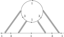
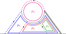
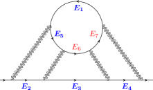
Figure A1: (a) A four-loop diagram with one fermion loop. The numbers next to the fermion lines represent the patch indices. (b) The four exclusive propagators are denoted as dashed lines. The remaining propagators represent the connected tree diagram. Loops (thick solid colored lines) are chosen such that each loop momentum goes through only one of the exclusive propagators. (c) The seven internal fermion propagators whose energies are denoted as $E_{l}$ with $1\leq l\leq 7$. $E_{1},E_{2},..,E_{5}$ are used as new integration variables along with $p_{i}^{{}^{\prime}}=cp_{i,x}$ with $i=1,2,3$, as discussed in the text.

The diagram in Figure A1 is a fermion self-energy with one fermion loop and three other loops, which we call ‘mixed loops’. For simplicity, we set the external momentum to zero. This does not affect the enhancement factors of $1/c$ and $1/v$ which originate from large internal momenta. We label the loop momenta as shown in Figure A1. With this choice, each mixed loop momentum $p_{i}$ with $i=1,2,3$ has a boson line that carries only $p_{i}$, and the fermion loop momentum $p_{4}$ has a fermion line that carries only $p_{4}$. These four propagators, denoted in Figure A1 by dashed lines, are called ‘exclusive propagators’. In the next section we show that it is always possible to find such exclusive propagators for every loop momentum in a general diagram. The diagram in Figure A1 is written as

$$I \sim v^{4}\int\prod_{r=1}^{4}dp_{r}\,\left(\prod_{j=1}^{3}\frac{1}{|p_{j,0}|+c(|p_{j,x}|+|p_{j,y}|)}\right)\times$$

$$\frac{1}{|p_{1,0}+p_{2,0}+p_{3,0}|+c(|p_{1,x}+p_{2,x}+p_{3,x}|+|p_{1,y}+p_{2,y}+p_{3,y}|)}\times$$

$$\frac{1}{ip_{4,0}+E_{1}}~{}~{}\frac{1}{ip_{1,0}+E_{2}}~{}~{}\frac{1}{i\left(p_{1,0}+p_{2,0}\right)+E_{3}}~{}~{}\frac{1}{i\left(p_{1,0}+p_{2,0}+p_{3,0}\right)+E_{4}}\times$$

$$\frac{1}{i(p_{4,0}-p_{1,0})+E_{5}}~{}~{}\frac{1}{i(p_{4,0}-p_{1,0}-p_{2,0})+E_{6}}~{}~{}\frac{1}{i(p_{4,0}-p_{1,0}-p_{2,0}-p_{3,0})+E_{7}},$$

where $p_{r}$ is the set of internal three-momenta, and $E_{i}$ represents the energy of the fermion in the $i$-th fermion propagator as denoted in Figure A1,

$$E_{1} = vp_{4,x}+p_{4,y},$$

$$E_{2} = vp_{1,x}-p_{1,y},$$

$$E_{3} = v(p_{1,x}+p_{2,x})+(p_{1,y}+p_{2,y}),$$

$$E_{4} = v(p_{1,x}+p_{2,x}+p_{3,x})-(p_{1,y}+p_{2,y}+p_{3,y}),$$

$$E_{5} = v(-p_{1,x}+p_{4,x})-(-p_{1,y}+p_{4,y}),$$

$$E_{6} = v(-p_{1,x}-p_{2,x}+p_{4,x})+(-p_{1,y}-p_{2,y}+p_{4,y}),$$

$$E_{7} = v(-p_{1,x}-p_{2,x}-p_{3,x}+p_{4,x})-(-p_{1,y}-p_{2,y}-p_{3,y}+p_{4,y}).$$ (A1)

Since frequency integrations are not affected by $v$ and $c$, we focus on the spatial components of momenta from now on. Our aim is to change the variables for the internal momenta so that the enhancement factors of $1/v$ and $1/c$ become manifest. As our first three new variables we choose $p_{j}^{{}^{\prime}}\equiv cp_{j,x}$ with $1\leq j\leq 3$. The last five variables are chosen to be $p_{l+3}^{{}^{\prime}}\equiv E_{l}$ with $1\leq l\leq 5$. The transformation between the old variables, written as $\{vp_{i,x},p_{i,y}\}$, and the new variables is given by

$$\left(\begin{array}[]{c}p_{1}^{{}^{\prime}}\\ p_{2}^{{}^{\prime}}\\ \vdots\\ p_{8}^{{}^{\prime}}\\ \end{array}\right)=\left(\begin{array}[]{cc}\frac{c}{v}{\mathbb{I}}_{3}&0\\ \tilde{\mathbb{A}}&\tilde{\mathbb{V}}\end{array}\right)\left(\begin{array}[]{c}vp_{1,x}\\ vp_{2,x}\\ vp_{3,x}\\ vp_{4,x}\\ p_{1,y}\\ p_{2,y}\\ p_{3,y}\\ p_{4,y}\\ \end{array}\right),$$ (A16)

where $\tilde{\mathbb{A}}$ and $\tilde{\mathbb{V}}$ are written as

$$\tilde{\mathbb{A}}=\left(\begin{array}[]{ccc}0&0&0\\ 1&0&0\\ 1&1&0\\ 1&1&1\\ -1&0&0\\ \end{array}\right),\hskip 14.22636pt\tilde{\mathbb{V}}=\left(\begin{array}[]{ccccc}1&0&0&0&1\\ 0&-1&0&0&0\\ 0&1&1&0&0\\ 0&-1&-1&-1&0\\ 1&1&0&0&-1\\ \end{array}\right),$$ (A27)

and ${\mathbb{I}}_{3}$ is the $3\times 3$ identity matrix. For non-zero $v,c$, the change of variables is non-degenerate, and the Jacobian of the transformation is $(2c^{3}v)^{-1}$. We show in the following section that such a non-degenerate choice is always possible for general diagrams. An easy mnemonic is that each fermion loop contributes a factor of $1/v$ because of nesting in the small $v$ limit, while each mixed loop contributes a factor of $1/c$ because of the vanishing boson velocity.

In the new coordinates, the momentum integration in Eq. (A-1) becomes

$$I \sim \frac{v^{3}}{c^{3}}\int\prod_{i=1}^{8}dp_{i}^{{}^{\prime}}\left(\prod_{j=1}^{3}\frac{1}{|p_{j}^{{}^{\prime}}|+O(c)}\right)\left(\prod_{l=4}^{8}\frac{1}{p_{l}^{{}^{\prime}}}\right)\tilde{R}[p^{{}^{\prime}}],$$ (A28)

where $\tilde{R}[p^{{}^{\prime}}]$ includes the propagators that are not explicitly shown. Now, we can safely take the small $c$ limit inside the integrand, because every momentum component has at least one propagator which guarantees that the integrand decays at least as $1/p_{j}^{{}^{\prime}}$ in the large momentum limit. Therefore, the integrations are UV convergent up to potential logarithmic divergences. To leading order in small $v$, the diagram scales as

$$I\sim\left(\frac{v}{c}\right)^{3}\sim v^{\frac{3}{2}}$$

up to potential logarithmic corrections.

A-2  General upper bound

Here we provide a general proof for the upper bound, by generalizing the example discussed in the previous section. We consider a general $L$-loop diagram that includes fermions from patches $1,3$,

$$I \sim v^{\frac{V}{2}}\int\prod_{r=1}^{L}dp_{r}\left(\prod_{l=1}^{I_{f}}\frac{1}{ik_{l,0}+vk_{l,x}+(-1)^{\frac{n_{l}-1}{2}}k_{l,y}}\right)\left(\prod_{m=1}^{I_{b}}\frac{1}{|q_{m,0}|+c(|q_{m,x}|+|q_{m,y}|)}\right).\hskip 28.45274pt$$ (A29)

Here $V$ is the number of vertices. $I_{f},I_{b}$ are the numbers of internal fermion and boson propagators, respectively. $p_{r}$ is the set of internal three-momenta. $k_{l}$ ($q_{m}$) represents the momentum that flows through the $l$-th fermion ($m$-th boson) propagator. These are linear combinations of the internal momenta and external momenta. The way $k_{l},q_{m}$ depend on $p_{r}$ is determined by how we choose internal loops within a diagram. $n_{l}=1,3$ is the patch index for the $l$-th fermion propagator. Since the frequency integrations are not affected by $v$ and $c$, we focus on the spatial components of momenta from now on.

It is convenient to choose loops in such a way that there exists a propagator exclusively assigned to each internal momentum. For this, we follow the procedure given in Sec. VI of Sur and Lee (2014). For a given diagram, we cut internal propagators one by one. We continue cutting until all loops disappear while the diagram remains connected. First, we cut one fermion propagator in every fermion loop, which requires cutting $L_{f}$ fermion lines. The remaining $L_{m}\equiv L-L_{f}$ loops, which we call mixed loops, can be removed by cutting boson propagators. After cutting $L$ lines in total, we are left with a connected tree diagram. Now we glue the propagators back one by one to restore the original $L$-loop diagram. Every time we glue one propagator, we assign one internal momentum such that it goes through the propagator that is just glued back and the connected tree diagram only. This guarantees that the propagator depends only on the internal momentum which is associated with the loop that is just formed by gluing. In gluing $L_{f}$ fermion propagators, the associated internal momenta go through the fermion loops. The $L_{m}$ mixed loops necessarily include both fermion and boson propagators. After all propagators are glued back, $L$ internal momenta are assigned in such a way that for every loop momentum there is one exclusive propagator.

With this choice of loops, Eq. (A29) is written as

$$I\sim v^{\frac{V}{2}}\int\prod_{r=1}^{L}dp_{r,x}dp_{r,y}\left(\prod_{j=1}^{L_{m}}\frac{1}{c|p_{j,x}|+c|p_{j,y}|}\right)\left(\prod_{l=1}^{I_{f}}\frac{1}{E_{l}(p)}\right)R[p].$$ (A30)

Here, frequency is suppressed, and IR divergences in the integrations over spatial momenta are understood to be cut off by frequencies. Our focus is on the UV divergence that arises in the spatial momentum integrations in the limit of small $v$ and $c$. The first group in the integrand represents the exclusive boson propagators assigned to the $L_{m}$ mixed loops. Each of the $L_{m}$ boson propagators depends on only one internal momentum due to the exclusive nature of our choice of loops. The second group represents all fermion propagators. $E_{l}(p)$ is the energy of the fermion in the $l$-th fermion propagator which is given by a linear superposition of $p_{r,x},p_{r,y}$. $R[p]$ represents the rest of the boson propagators that are not assigned as exclusive propagators.

Our strategy is to find a new basis for the loop momenta such that the divergences in the small $v$ and $c$ limit become manifest. The first $L_{m}$ variables are chosen to be $cp_{j,x}$ with $j=1,2,..,L_{m}$ while the remaining $2L-L_{m}$ variables are chosen among $\{E_{l}(p)\}$. This is possible because $I_{f}\geq(2L-L_{m})$ for diagrams with $E>0$. We express $p_{j}^{{}^{\prime}}\equiv cp_{j,x}$ and $E_{l}(p)$ in terms of $vp_{r,x},p_{r,y}$,

$$\left(\begin{array}[]{c}p_{1}^{{}^{\prime}}\\ p_{2}^{{}^{\prime}}\\ \vdots\\ p_{L_{m}}^{{}^{\prime}}\\ E_{1}\\ E_{2}\\ \vdots\\ E_{I_{f}}\end{array}\right)=\left(\begin{array}[]{cc}\frac{c}{v}{\mathbb{I}}_{L_{m}}&0\\ {\mathbb{A}}&{\mathbb{V}}\end{array}\right)\left(\begin{array}[]{c}vp_{1,x}\\ vp_{2,x}\\ \vdots\\ vp_{L_{m},x}\\ vp_{L_{m}+1,x}\\ \vdots\\ vp_{L,x}\\ p_{1,y}\\ p_{2,y}\\ \vdots\\ p_{L,y}\\ \end{array}\right).$$ (A52)

Here ${\mathbb{I}}_{a}$ is the $a\times a$ identity matrix. $A_{l,j}=\frac{1}{v}\frac{\partial E_{l}}{\partial p_{j,x}}$ with $1\leq l\leq I_{f}$, $1\leq j\leq L_{m}$. ${\mathbb{V}}$ is an $I_{f}\times(2L-L_{m})$ matrix whose first $L-L_{m}$ columns are given by $V_{l,i-L_{m}}=\frac{1}{v}\frac{\partial E_{l}}{\partial p_{i,x}}$ with $L_{m}+1\leq i\leq L$ and the remaining $L$ columns are given by $V_{l,i+(L-L_{m})}=\frac{\partial E_{l}}{\partial p_{i,y}}$ with $1\leq i\leq L$. Now we focus on the lower-right corner of the transformation matrix which governs the relation between $\vec{E}^{T}\equiv(E_{1},E_{2},..,E_{I_{f}})$ and $\vec{P}^{T}\equiv(vp_{L_{m}+1,x},..,vp_{L,x},p_{1,y},..,p_{L,y})$ when $p_{j,x}=0$ for $1\leq j\leq L_{m}$,

$$\vec{E}={\mathbb{V}}\vec{P}.$$ (A53)

$\vec{P}$ represents the $x,y$ components of momenta in the fermion loops and the $y$ components of momenta in the mixed loops. The matrix ${\mathbb{V}}$ can be viewed as a collection of $2L-L_{m}$ column vectors, each of which have $I_{f}$ components. We first show that the $2L-L_{m}$ column vectors are linearly independent.

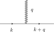
Figure A2: For a boson momentum $\vec{q}$, there exists a unique $\vec{k}$ such that $\varepsilon_{1}(\vec{k})=\varepsilon_{3}(\vec{k}+\vec{q})=0$ for $v\neq 0$.

If the column vectors were not linearly independent, there would exist a nonzero $\vec{P}$ such that ${\mathbb{V}}\vec{P}=0$. This implies that there exists at least a one-parameter family of $x,y$-momenta in the $L_{f}$ fermion loops and $y$-momenta in the $L_{m}$ mixed loops such that all internal fermions lie on the Fermi surface. However, this is impossible for the following reason. For $v\neq 0$, a momentum on an external boson leg uniquely fixes the internal momenta on the two fermion lines attached to the boson line if both fermions are required to have zero energy. This is illustrated in Figure A2. Similarly, a momentum on an external fermion leg fixes the momenta on the adjacent internal fermion and boson lines if the internal fermion is required to have zero energy and only the $y$ component of momentum is allowed to vary in the mixed loops. Once the momenta on the internal lines attached to the external lines are fixed, those internal lines in turn fix the momenta of other adjoining internal lines. As a result, all internal momenta are successively fixed by external momenta if we require that $E_{l}=0$ for all $l$. Therefore, there cannot be a non-trivial $\vec{P}$ that satisfies ${\mathbb{V}}\vec{P}=0$. This implies that the column vectors in ${\mathbb{V}}$ must be linearly independent.

Since ${\mathbb{V}}$ is made of $(2L-L_{m})$ independent column vectors, it necessarily includes $(2L-L_{m})$ independent row vectors. Let the $l_{k}$-th rows with $k=1,2,..,(2L-L_{m})$ be the set of rows that are linearly independent, and $\tilde{\mathbb{V}}$ be a $(2L-L_{m})\times(2L-L_{m})$ invertible matrix made of these rows. We choose $p_{L_{m}+k}^{{}^{\prime}}\equiv E_{l_{k}}$ with $k=1,2,..,(2L-L_{m})$ as the remaining $(2L-L_{m})$ integration variables. The transformation between the original $2L$ momentum variables and the new variables is given by

$$\left(\begin{array}[]{c}p_{1}^{{}^{\prime}}\\ p_{2}^{{}^{\prime}}\\ \vdots\\ p_{2L}^{{}^{\prime}}\\ \end{array}\right)=\left(\begin{array}[]{cc}\frac{c}{v}{\mathbb{I}}_{L_{m}}&0\\ \tilde{\mathbb{A}}&\tilde{\mathbb{V}}\end{array}\right)\left(\begin{array}[]{c}vp_{1,x}\\ vp_{2,x}\\ \vdots\\ vp_{L,x}\\ p_{1,y}\\ p_{2,y}\\ \vdots\\ p_{L,y}\\ \end{array}\right),$$ (A68)

where $\tilde{\mathbb{A}}$ is a $(2L-L_{m})\times L_{m}$ matrix made of the collection of the $l_{k}$-th rows of ${\mathbb{A}}$ with $k=1,2,..,(2L-L_{m})$. The Jacobian of the transformation is given by $Y^{-1}c^{-L_{m}}v^{-L_{f}}$. Here, $Y=|\det\tilde{\mathbb{V}}|$ is a constant independent of $v$ and $c$, which is nonzero because $\tilde{\mathbb{V}}$ is invertible.

In the new variables, Eq. (A30) becomes

$$I \sim v^{\frac{V}{2}-L_{f}}c^{-L_{m}}\int\prod_{i=1}^{2L}dp_{i}^{{}^{\prime}}\left(\prod_{j=1}^{L_{m}}\frac{1}{|p_{j}^{{}^{\prime}}|+O(c)}\right)\left(\prod_{l=L_{m}+1}^{2L}\frac{1}{p_{l}^{{}^{\prime}}}\right)\tilde{R}[p^{{}^{\prime}}].$$ (A69)

Every component of the loop momenta has at least one propagator which guarantees that the integrand decays at least as $1/p^{{}^{\prime}}_{l}$ in the large momentum limit. $\tilde{R}[p^{{}^{\prime}}]$ is the product of all remaining propagators. Therefore, the integrations over the new variables are convergent up to potentially logarithmic divergences. Using $L=\frac{1}{2}(V+2-E)$, one can see that a general diagram is bounded by

$$I\sim v^{\frac{E-2}{2}}\left(\frac{v}{c}\right)^{L-L_{f}}$$ (A70)

up to logarithmic corrections. Diagrams with large $(L-L_{f})$ are systematically suppressed for $v\ll c$. This bound can be checked explicitly for individual diagrams.

Appendix B Derivation of the self-consistent boson self-energy

In this section, we derive Eqs. (5) and (6) from Eq. (8).

The one-loop quantum effective action of the boson generated from Fig. 3 is written as

$$\Gamma^{1L}_{(0,2)}=\frac{1}{4}\int dq~{}\Pi^{1L}(q)~{}\text{Tr}\left[\Phi(-q)\Phi(q)\right],$$ (B71)

where

$$\Pi^{1L}(q)=-\pi v\sum_{n=1}^{4}\int dk~{}\text{Tr}\left[\gamma_{1}G_{n}^{(0)}(k)\gamma_{1}G_{\bar{n}}^{(0)}(k+q)\right]$$ (B72)

and the bare fermion propagator is $G_{n}^{(0)}(k)=-i\frac{k_{0}\gamma_{0}+\varepsilon_{n}(\vec{k})\gamma_{1}}{k_{0}^{2}+\varepsilon_{n}^{2}(\vec{k})}$ and $dk\equiv\frac{d^{3}k}{(2\pi)^{3}}$. The integration of the spatial momentum gives $\Pi^{1L}(q)=-\frac{1}{2}\int dk_{0}\frac{(k_{0}+q_{0})k_{0}}{|k_{0}+q_{0}||k_{0}|}$. The $k_{0}$ integration generates a linearly divergent mass renormalization which is removed by a counter term, and a finite self-energy,

$$\Pi^{1L}=|q_{0}|.$$ (B73)

Since the one-loop self-energy depends only on frequency, we have to include higher-loop diagrams to generate a momentum-dependent quantum effective action, even though they are suppressed by powers of $v$ compared to the one-loop self-energy. According to Eq. (7), the next leading diagrams are the ones with $L-L_{f}=1$. Among the diagrams with $L-L_{f}=1$, the only one that contributes to the momentum-dependent boson self-energy is shown in Figure 3. In particular, other two-loop diagrams that include fermion self-energy insertions do not contribute. Since the two-loop diagram itself depends on the unknown dressed boson propagator, we need to solve the self-consistent equation for $D(q)$ in Eq. (8). Here, we first assume that the solution takes the form of Eq. (5) with $v\ll c\ll 1$ to compute the two-loop contribution, and show that the resulting boson propagator agrees with the assumed one. The two-loop self-energy reads

$$\begin{split}\Pi^{2L}(q)=-\frac{\pi^{2}v^{2}}{2}\sum^{4}_{n=1}\int\mathrm{d}k\mathrm{d}p\left[\frac{1}{\left(k_{0}+p_{0}-i\varepsilon_{n}(\vec{k}+\vec{p})\right)\left(k_{0}-i\varepsilon_{\bar{n}}(\vec{k})\right)}\right.\\ \left.\times\frac{1}{\left(k_{0}+q_{0}-i\varepsilon_{n}(\vec{k}+\vec{q})\right)\left(k_{0}+p_{0}+q_{0}-i\varepsilon_{\bar{n}}(\vec{k}+\vec{p}+\vec{q})\right)}\right]D(p)+\mathrm{c.c.}.\end{split}$$ (B74)

Here c.c. denotes the complex conjugate. Straightforward integrations over $\vec{k}$ and $k_{0}$ give

$$\Pi^{2L}(q_{0},\vec{q})=-\frac{\pi v}{8}\sum^{4}_{n=1}\int\mathrm{d}p\left[\frac{|q_{0}|-|p_{0}|}{((p_{0}+q_{0})-i\varepsilon_{\bar{n}}(\vec{p}+\vec{q}))((q_{0}-p_{0})-i\varepsilon_{n}(\vec{q}-\vec{p}))}\right]D(p)+\mathrm{c.c.}.$$ (B75)

Since the frequency-dependent self-energy is already generated from the lower order one-loop graph in Figure 3, we focus on the momentum-dependent part. This allows us to set the external frequency to zero to rewrite Eq. (B75) as

$$\Pi^{2L}(0,\vec{q})=\frac{\pi v}{4}\sum^{4}_{n=1}\int\mathrm{d}p\left[\frac{|p_{0}|}{(ip_{0}+\varepsilon_{\bar{n}}(\vec{p}+\vec{q}))(ip_{0}+\varepsilon_{n}(\vec{p}-\vec{q}))}\right]D(p).$$ (B76)

After subtracting the linearly divergent mass renormalization, $\Delta\Pi^{2L}(0,\vec{q})\equiv\Pi^{2L}(0,\vec{q})-\Pi^{2L}(0,0)$ is UV finite,

$$\Delta\Pi^{2L}(0,\vec{q})=\frac{\pi v}{4}\sum^{4}_{n=1}\int\mathrm{d}p\frac{|p_{0}|\mathcal{F}^{1L(n)}(p_{0},\vec{p},\vec{q};v)}{(p^{2}_{0}+\varepsilon^{2}_{\bar{n}}(\vec{p}+\vec{q}))(p^{2}_{0}+\varepsilon^{2}_{n}(\vec{p}-\vec{q}))(p^{2}_{0}+\varepsilon^{2}_{\bar{n}}(\vec{p}))(p^{2}_{0}+\varepsilon^{2}_{n}(\vec{p}))}D(p),$$ (B77)

where

$$\begin{split}\mathcal{F}^{1L(n)}(p_{0},\vec{p},\vec{q};v)&=(p^{2}_{0}+\varepsilon^{2}_{n}(\vec{p}))(p^{2}_{0}+\varepsilon^{2}_{\bar{n}}(\vec{p}))(ip_{0}-\varepsilon_{\bar{n}}(\vec{p}+\vec{q}))(ip_{0}-\varepsilon_{n}(\vec{p}-\vec{q}))\\ &-(p^{2}_{0}+\varepsilon^{2}_{\bar{n}}(\vec{p}+\vec{q}))(p^{2}_{0}+\varepsilon^{2}_{n}(\vec{p}-\vec{q}))(ip_{0}-\varepsilon_{\bar{n}}(\vec{p}))(ip_{0}-\varepsilon_{n}(\vec{p})).\end{split}$$ (B78)

Now we consider the contribution of each hot spot separately. For $n=1$, the dependence on $q_{x}$ is suppressed by $v$ compared to the $q_{y}$-dependent self-energy. Therefore, we set $q_{x}=0$ for small $v$. Furthermore, the $p_{y}$ dependence in $D(p)$ can be safely dropped in the small $c$ limit because $\varepsilon_{1}(\vec{p})$ and $\varepsilon_{3}(\vec{p})$ suppress the contributions from large $p_{y}$. Rescaling the momentum as $(p_{0},p_{x},p_{y})\rightarrow|q_{y}|(p_{0},p_{x}/c,p_{y})$ followed by the integration over $p_{y}$, we obtain the contribution from the hot spot $n=1$,

$$\Delta\Pi^{2L}(0,\vec{q}) =\frac{v}{32\pi c}|q_{y}|\int\mathrm{d}p_{0}\mathrm{d}p_{x}\frac{(1+p^{2}_{0}-3p^{2}_{x}w^{2})p^{2}_{0}}{(p^{2}_{0}+w^{2}p^{2}_{x})(p^{2}_{0}+(wp_{x}-1)^{2})(p^{2}_{0}+(wp_{x}+1)^{2})}\frac{1}{|p_{0}|+|p_{x}|},$$ (B79)

where $w\equiv v/c$. In the integrand, we can not set $w=0$ because the integration over $p_{x}$ is logarithmically divergent in the small $w$ limit,

$$\begin{split}&\Delta\Pi^{2L(1)}(0,\vec{q})=\frac{v}{32\pi c}|q_{y}|\int\mathrm{d}p_{0}\frac{1}{1+p^{2}_{0}}\left[-2\log(w)-2p_{0}\cot^{-1}(p_{0})+p_{0}^{2}\log\left(\frac{p^{2}_{0}}{1+p^{2}_{0}}\right)+O(w)\right].\end{split}$$ (B80)

Finally, the integration over $p_{0}$ gives

$$\Delta\Pi^{2L(1)}(0,\vec{q}) =\frac{|q_{y}|v}{16c}\left[\log\left(\frac{1}{w}\right)-1+O(w)\right].$$ (B81)

In the small $w$ limit, the first term dominates. Hot spot $3$ generates the same term, and the contribution from hot spots $2,4$ is obtained by replacing $q_{y}$ with $q_{x}$. Summing over contributions from all the hot spots, we obtain

$$\Delta\Pi^{2L}(0,\vec{q}) =\frac{v}{8c}\log\left(\frac{c}{v}\right)\left(|q_{x}|+|q_{y}|\right)+O\left(\frac{1}{vc}\right).$$ (B82)

The two-loop diagram indeed reproduces the assumed form of the self-energy which is proportional to $|q_{x}|+|q_{y}|$ to the leading order in $v$. The full Schwinger-Dyson equation now boils down to a self-consistent equation for the boson velocity,

$$c=\frac{v}{8c}\log\left(\frac{c}{v}\right).$$ (B83)

$c$ is solved in terms of $v$ as

$$c(v)=\frac{1}{4}\sqrt{v\log\left(\frac{1}{v}\right)}\left(1+O\left(\frac{\log\log(1/v)}{\log(1/v)}\right)\right).$$ (B84)

This is consistent with the assumption that $v\ll c\ll 1$ in the small $v$ limit.

The full propagator of the boson which includes the bare kinetic term in Eq. (1) is given by

$$D(q)^{-1}=|q_{0}|+c(|q_{x}|+|q_{y}|)+\frac{q_{0}^{2}}{\tilde{\Lambda}}+\frac{c_{0}^{2}}{\tilde{\Lambda}}|\vec{q}|^{2},$$ (B85)

where $\tilde{\Lambda}$ is a UV scale associated with the coupling. Depending on the ratio between $c$ and $c_{0}$, which is determined by microscopic details, one can have different sets of crossovers.

energy	scaling	dynamical critical exponent
$q_{0}>\tilde{\Lambda}$	$q_{0}\sim c_{0}q$	$z=1$
$\frac{c^{2}}{c_{0}^{2}}\tilde{\Lambda}<q_{0}<\tilde{\Lambda}$	$q_{0}\sim c_{0}^{2}q^{2}/\tilde{\Lambda}$	$z=2$
$q_{0}<\frac{c^{2}}{c_{0}^{2}}\tilde{\Lambda}$	$q_{0}\sim cq$	$z=1$

Table B1: The energy dependent dynamical critical exponent for $c_{0}>c$.

energy	scaling	dynamical critical exponent
$q_{0}>\frac{c}{c_{0}}\tilde{\Lambda}$	$q_{0}\sim c_{0}q$	$z=1$
$\tilde{\Lambda}<q_{0}<\frac{c}{c_{0}}\tilde{\Lambda}$	$q_{0}\sim\sqrt{c\tilde{\Lambda}q}$	$z=\frac{1}{2}$
$q_{0}<\tilde{\Lambda}$	$q_{0}\sim cq$	$z=1$

Table B2: The energy dependent dynamical critical exponent for $c_{0}<c$.

For $c_{0}>c$, one has a series of crossovers from the Gaussian scaling with $z=1$ at high energies, to the scaling with $z=2$ at intermediate energies and to the non-Fermi liquid scaling with $z=1$ at low energies. In the low energy limit, the system eventually becomes superconducting. For $c_{0}<c$, on the other hand, the $z=2$ scaling is replaced with a scaling with $z=\frac{1}{2}$ at intermediate energies. This is summarized in Tables B1 and B2.

Appendix C Derivation of the beta function for $v$

In this section, we derive the beta function for $v$ in Eq. (11). We first compute the counter terms that need to be added to the local action such that the quantum effective action is independent of the UV cut-off scale to the lowest order in $v$. Then we derive the beta function for $v$ and its solution, which confirms that $v$ flows to zero in the low-energy limit.

C-1  Frequency-dependent fermion self-energy

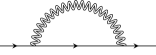
Figure C3: The one-loop diagram for the fermion self-energy.

According to Eq. (7), the leading order fermion self-energy is generated from Fig. C3 in the small $v$ limit. The one-loop fermion self-energy for patch $n$ is given by

$$\Sigma^{1L(n)}(k_{0},\vec{k})=\frac{3\pi v}{2}\int dp~{}\gamma_{1}G_{\bar{n}}^{(0)}(p+k)\gamma_{1}D(p),$$ (C86)

where the dressed boson propagator is $D(p)=\frac{1}{|p_{0}|+c(v)(|p_{x}|+|p_{y}|)}$. We first compute $\Sigma^{1L(n)}(k)$ for $n=1$. The quantum correction is logarithmically divergent, and a UV cut-off $\Lambda$ is imposed on $p_{y}$, which is the momentum perpendicular to the Fermi surface for $n=1$ in the small $v$ limit. However, the logarithmically divergent term is independent of how UV cut-off is implemented. To extract the frequency-dependent self-energy, we set $\vec{k}=0$ and rescale $(p_{0},p_{x},p_{y})\rightarrow|k_{0}|(p_{0},p_{x}/c,p_{y})$ to rewrite

$$\Sigma^{1L(1)}(k_{0},0) =i\gamma_{0}k_{0}\frac{3\pi v}{2c}\int dp~{}\frac{p_{0}+1}{\left[(p_{0}+1)^{2}+(wp_{x}-p_{y})^{2}\right]\left[|p_{0}|+|p_{x}|+c|p_{y}|\right]},$$ (C87)

where $w=\frac{v}{c}$. Under this rescaling, the UV cut-off for $p_{y}$ is also rescaled to $\Lambda_{0}=\Lambda/|k_{0}|$. The $p_{0}$ integration gives

$$\Sigma^{1L(1)}(k_{0},0)=i\gamma_{0}k_{0}\frac{3\pi v}{2(2\pi)^{3}c}\int_{-\Lambda_{0}}^{\Lambda_{0}}dp_{y}\int dp_{x}$$

$$\left[\frac{\pi}{2}|p_{y}-wp_{x}|\left(\frac{1}{(p_{y}-wp_{x})^{2}+(-1+|p_{x}|+c|p_{y}|)^{2}}-\frac{1}{(p_{y}-wp_{x})^{2}+(1+|p_{x}|+c|p_{y}|)^{2}}\right)\right.$$

$$-\left.(p_{y}-wp_{x})\operatorname{arccot}(p_{y}-wp_{x})\left(\frac{1}{(p_{y}-wp_{x})^{2}+(-1+|p_{x}|+c|p_{y}|)^{2}}+\frac{1}{(p_{y}-wp_{x})^{2}+(1+|p_{x}|+c|p_{y}|)^{2}}\right)\right.$$

$$+\left.\frac{1}{2}\log\left(\frac{1+(p_{y}-wp_{x})^{2}}{(|p_{x}|+c|p_{y}|)^{2}}\right)\left(\frac{1+|p_{x}|+c|p_{y}|}{(p_{y}-wp_{x})^{2}+(1+|p_{x}|+c|p_{y}|)^{2}}-\frac{-1+|p_{x}|+c|p_{y}|}{(p_{y}-wp_{x})^{2}+(-1+|p_{x}|+c|p_{y}|)^{2}}\right)\right].$$ (C88)

The logarithmically divergent contribution is obtained to be

$$\Sigma^{1L(1)}(k_{0},0) =\frac{3}{4\pi}\frac{v}{c}\log\left(\frac{\Lambda}{|k_{0}|}\right)i\gamma_{0}k_{0}$$ (C89)

in the small $v$ limit. The self-energy for other patches is obtained from a series of $90$-degree rotations, and the frequency-dependent part is identical for all patches. In order to remove the cut-off dependence in the quantum effective action, we add the counter term,

$$\sum_{n=1}^{4}\sum_{\sigma=\uparrow,\downarrow}\int dk~{}\bar{\Psi}_{n,\sigma}(k)\left(Z_{1,1}\,i\gamma_{0}k_{0}\right)\Psi_{n,\sigma}(k)$$ (C90)

with

$$Z_{1,1}=-\frac{3}{4\pi}\frac{v}{c}\,\log\left(\frac{\Lambda}{\mu}\right),$$ (C91)

where $\mu$ is the scale at which the quantum effective action is defined in terms of the renormalized velocity $v$. The counter term guarantees that the renormalized propagator at the scale $\mu$ is expressed solely in terms of $v$ in the $\Lambda/\mu\rightarrow\infty$ limit.

C-2  Momentum-dependent fermion self-energy

To compute the momentum-dependent fermion self-energy, we start with Eq. (C86) for $n=1$ and set $k_{0}=0$. Rescaling $p_{x}\rightarrow\frac{p_{x}}{c}$ gives

$$\Sigma^{1L(1)}(0,\vec{k})=-\frac{3\pi v}{2c}i\gamma_{1}\int dp~{}\frac{wp_{x}-p_{y}+\varepsilon_{3}(\vec{k})}{\left[p_{0}^{2}+(wp_{x}-p_{y}+\varepsilon_{3}(\vec{k}))^{2}\right]\left[|p_{0}|+|p_{x}|+c|p_{y}|\right]}.$$ (C92)

The integration over $p_{0}$ results in $\Sigma^{1L(1)}(0,\vec{k})=\left.\Sigma^{1L(1)}(\vec{k})\right|_{\text{term 1}}+\left.\Sigma^{1L(1)}(\vec{k})\right|_{\text{term 2}}$, where

$$\left.\Sigma^{1L(1)}(\vec{k})\right|_{\text{term 1}}= -i\gamma_{1}\frac{3\pi v}{2(2\pi)^{3}c}\int dp_{y}\int dp_{x}\frac{\mathrm{sgn}(wp_{x}-p_{y}+\varepsilon_{3}(\vec{k}))(|p_{x}|+c|p_{y}|)\pi}{(p_{y}-\varepsilon_{3}(\vec{k})-wp_{x})^{2}+(|p_{x}|+c|p_{y}|)^{2}},$$ (C93)

$$\left.\Sigma^{1L(1)}(\vec{k})\right|_{\text{term 2}}= -i\gamma_{1}\frac{3\pi v}{2(2\pi)^{3}c}\int dp_{y}\int dp_{x}\frac{(p_{y}-\varepsilon_{3}(\vec{k})-wp_{x})\log\left(\frac{(|p_{x}|+c|p_{y}|)^{2}}{(p_{y}-\varepsilon_{3}(\vec{k})-wp_{x})^{2}}\right)}{(p_{y}-\varepsilon_{3}(\vec{k})-wp_{x})^{2}+(|p_{x}|+c|p_{y}|)^{2}}.$$ (C94)

We first compute the first term. After performing the $p_{x}$ integration, we rescale $p_{y}\rightarrow|\varepsilon_{3}(\vec{k})|p_{y}$ to obtain

$$\left.\Sigma^{1L(1)}(\vec{k})\right|_{\text{term 1}}=-\frac{3\pi^{2}v}{2(2\pi)^{3}c}i\gamma_{1}\varepsilon_{3}(\vec{k})\int_{-\Lambda_{3}}^{\Lambda_{3}}dp_{y}\Bigg{[}\frac{\pi w}{2(1+w^{2})}\left(\mathrm{sgn}\left(p_{y}-1+cw|p_{y}|\right)+\mathrm{sgn}\left(p_{y}-1-cw|p_{y}|\right)\right)$$

$$+\frac{\mathrm{sgn}\left(p_{y}-1\right)}{1+w^{2}}\left(w\arctan\left(\frac{w\left(-p_{y}+1\right)+c|p_{y}|}{p_{y}-1+cw|p_{y}|}\right)+w\arctan\left(\frac{w\left(p_{y}-1\right)+c|p_{y}|}{-p_{y}+1+cw|p_{y}|}\right)\right.$$

$$-\left.2w\arctan\left(w^{-1}\right)-\log\left(\frac{c^{2}w^{2}p_{y}^{2}+\left(p_{y}-1\right)^{2}+2cw\left|p_{y}-1\right||p_{y}|}{w^{2}\left(c^{2}p_{y}^{2}+\left(p_{y}-1\right)^{2}\right)}\right)\right)\Bigg{]},$$ (C95)

where $\Lambda_{3}=\frac{\Lambda}{|\varepsilon_{3}(\vec{k})|}$. The remaining $p_{y}$ integration gives

$$\left.\Sigma^{1L(1)}(\vec{k})\right|_{\text{term 1}}=\frac{3v(w-c)}{4\pi}\log\left(\frac{\Lambda}{|\varepsilon_{3}(\vec{k})|}\right)i\gamma_{1}\varepsilon_{3}(\vec{k})$$ (C96)

to the leading order in $v$ up to terms that are finite in the large $\Lambda$ limit.

The second term can be computed similarly in the small $v$ limit,

$$\left.\Sigma^{1L(1)}(\vec{k})\right|_{\text{term 2}}=-\frac{3}{2\pi^{2}}\,v\log\left(\frac{1}{c}\right)\log\left(\frac{\Lambda}{|\varepsilon_{3}(\vec{k})|}\right)i\gamma_{1}\varepsilon_{3}(\vec{k})$$ (C97)

up to UV-finite terms. It is noted that the second term is dominant for small $v$.

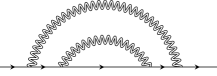
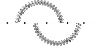
Figure C4: Two-loop diagrams for the fermion self-energy. While (a) is sub-leading in the small $v$ limit, (b) is of the same order as Figure C3.

According to Eq. (7), the upper bound for the one-loop fermion self-energy is $v/c$. However, Eq. (C97) is strictly smaller than the upper bound. The extra suppression by $c$ arises due to the fact that the external momentum in Figure C3 can be directed to flow only through the boson propagator, and the diagram becomes independent of the external momentum in the small $c$ limit. Since this suppression does not happen for higher-loop diagrams in general, the one-loop diagram becomes comparable to some two-loop diagrams with $L-L_{f}=2$. Therefore, we have to include the two-loop diagrams for the self-energy in order to capture all leading order corrections. The rainbow diagram in Figure C4 is smaller for the same reason as the one-loop diagram. Three and higher-loop diagrams remain negligible, and only Figure C4 contributes to the leading order. The two-loop self-energy for patch $n$ is given by

$$\Sigma^{2L(n)}(k_{0},\vec{k})=\frac{3\pi^{2}v^{2}}{4}\int dpdq~{}\left[\gamma_{1}G_{\bar{n}}(k+q)\gamma_{1}G_{n}(k+q+p)\gamma_{1}G_{\bar{n}}(k+p)\gamma_{1}\right]D(q)D(p).$$ (C98)

It is noted that $\Sigma^{2L(n)}(k_{0},0)$ is strictly smaller than $\Sigma^{1L(n)}(k_{0},0)$, and only $\Sigma^{2L(n)}(0,\vec{k})$ is of the same order as $\Sigma^{1L(n)}(0,\vec{k})$. Therefore, we only compute $\Sigma^{2L(n)}(0,\vec{k})$. After performing the integrations over $p_{y},q_{y}$, the self-energy for patch $1$ becomes

$$\Sigma^{2L(1)}(0,\vec{k})= -\frac{3v^{2}}{2^{8}\pi^{2}c^{2}}i\gamma_{1}\int dp_{0}\int dq_{0}~{}(\mathrm{sgn}(p_{0})+\mathrm{sgn}(p_{0}+q_{0}))(\mathrm{sgn}(q_{0})+\mathrm{sgn}(2p_{0}+q_{0}))\times$$

$$\int dp_{x}\int dq_{x}~{}\frac{2w(p_{x}+q_{x})+(3vk_{x}-k_{y})}{4(p_{0}+q_{0})^{2}+(2w(p_{x}+q_{x})+(3vk_{x}-k_{y}))^{2}}\frac{1}{|p_{0}|+|p_{x}|}\frac{1}{|q_{0}|+|q_{x}|}.$$ (C99)

We single out the factor of $(3vk_{x}-k_{y})$ by rescaling $(p_{0},p_{x},q_{0},q_{x})\rightarrow|3vk_{x}-k_{y}|(p_{0},p_{x},q_{0},q_{x})$. To perform the $p_{x}$ and $q_{x}$ integrals, we introduce variables $a=\frac{1}{2}(p_{x}+q_{x}),b=\frac{1}{2}(p_{x}-q_{x})$. After the straightforward integration over $b$, we rescale $a\rightarrow\frac{a}{w}$ to obtain

$$\Sigma^{2L(1)}(0,\vec{k}) =-\frac{3v^{2}}{2^{7}\pi^{2}c^{2}}i\gamma_{1}(3vk_{x}-k_{y})\int dp_{0}\int dq_{0}$$

$$(\mathrm{sgn}(p_{0})+\mathrm{sgn}(p_{0}+q_{0}))(\mathrm{sgn}(q_{0})+\mathrm{sgn}(2p_{0}+q_{0}))\int da~{}\frac{4a+1}{4(p_{0}+q_{0})^{2}+(4a+1)^{2}}\times$$

$$\left(\frac{\log\left(\frac{(2|a|+w|p_{0}|)(2|a|+w|q_{0}|)}{w^{2}|p_{0}||q_{0}|}\right)}{2|a|+w(|p_{0}|+|q_{0}|)}-\frac{\log\left(\frac{w|q_{0}|}{2|a|+w|p_{0}|}\right)}{2|a|+w(|p_{0}|-|q_{0}|)}-\frac{\log\left(\frac{w|p_{0}|}{2|a|+w|q_{0}|}\right)}{2|a|-w(|p_{0}|-|q_{0}|)}\right),$$ (C100)

where the frequency integrations are understood to have a UV cut-off, $\Lambda_{3}^{{}^{\prime}}=\frac{\Lambda}{|3vk_{x}-k_{y}|}$ in the rescaled variable. In the small $w$ limit, the $a$ integration diverges as $(\log(w))^{2}$. The sub-leading terms are suppressed compared to the one-loop diagram, and we drop them in the small $w$ limit. The remaining frequency integrations are logarithmically divergent in the UV cut-off,

$$\Sigma^{2L(1)}(0,\vec{k})=-i\gamma_{1}\frac{3}{32\pi^{2}}\left(\frac{v}{c}\log\frac{c}{v}\right)^{2}\log\left(\frac{\Lambda}{|3vk_{x}-k_{y}|}\right)\left(3vk_{x}-k_{y}\right).$$ (C101)

This is of the same order as Eq. (C97) because of $\left(\frac{v}{c}\log\frac{c}{v}\right)^{2}=8v\log\frac{1}{c}$ to the leading order in $v$.

The vertex correction in Figure C4 strengthens the bare vertex, and the two-loop self-energy has the same sign as the one-loop self-energy. In particular, both the one-loop and two-loop quantum corrections enhance nesting, and drive $v$ to a smaller value at low energies. To remove the cut-off dependences of Eq. (C97) and Eq. (C101) in the quantum effective action, we add the counter term

$$\sum_{\sigma=\uparrow,\downarrow}\int dk~{}\bar{\Psi}_{1,\sigma}(k)\left(i\gamma_{1}(Z_{2,1}vk_{x}+Z_{3,1}k_{y})\right)\Psi_{1,\sigma}(k)$$ (C102)

with

$$Z_{2,1} = \frac{15}{4\pi^{2}}v\,\log\left(\frac{1}{c}\right)\,\log\left(\frac{\Lambda}{\mu}\right),$$

$$Z_{3,1} = -\frac{9}{4\pi^{2}}v\,\log\left(\frac{1}{c}\right)\,\log\left(\frac{\Lambda}{\mu}\right).$$ (C103)

Counter terms for $n=2,3,4$ are fixed by the four-fold rotational symmetry.

C-3  Vertex correction

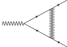
Figure C5: The one-loop diagram for the vertex correction.

The one-loop vertex correction in Fig. C5 is given by

$$\Gamma^{1L}(k,q) =\frac{\pi v}{2}\int dp~{}\gamma_{1}G_{\bar{n}}^{(0)}(p+k+q)\gamma_{1}G_{n}^{(0)}(p+k)\gamma_{1}D(p).$$ (C104)

We set all external momenta to zero except for $k_{0}$, which plays the role of an IR regulator. For $n=1$, it is convenient to rescale $(p_{0},p_{x},p_{y})\rightarrow|k_{0}|(p_{0},p_{x}/c,p_{y})$. The $p_{0}$ integration gives

$$\Gamma^{1L(1)}(k_{0})=\frac{\pi v}{2c}\gamma_{1}\frac{1}{(2\pi)^{3}}\int_{-\Lambda_{0}}^{\Lambda_{0}}dp_{y}\int dp_{x}$$

$$\frac{\left\{\begin{aligned} &\left[\left((p_{y}-wp_{x})(p_{y}+wp_{x})^{3}+(-1+(|p_{x}|+c|p_{y}|)^{2})^{2}\right)\left(1+(p_{y}-wp_{x})^{2}+(|p_{x}|+c|p_{y}|)^{2}\right)\right.+\\ &\left.\left.(p_{y}-wp_{x})(p_{y}+wp_{x})\left(1+6(|p_{x}|+c|p_{y}|)^{2}+(|p_{x}|+c|p_{y}|)^{4}+(p_{y}-wp_{x})^{2}(1+(|p_{x}|+c|p_{y}|)^{2})\right)\right.\right.\\ &\left.+(p_{y}+wp_{x})^{2}\left((-1+(|p_{x}|+c|p_{y}|)^{2})^{2}+(p_{y}-wp_{x})^{2}(1+(|p_{x}|+c|p_{y}|)^{2})\right)\right]\log(|p_{x}|+c|p_{y}|)\end{aligned}\right\}}{-\frac{1}{2}\left\{\begin{aligned} &\left((p_{y}-wp_{x})^{2}+(-1+|p_{x}|+c|p_{y}|)^{2}\right)\left((p_{y}+wp_{x})^{2}+(-1+|p_{x}|+c|p_{y}|)^{2}\right)\\ &\times\left((p_{y}-wp_{x})^{2}+(1+|p_{x}|+c|p_{y}|)^{2}\right)\left((p_{y}+wp_{x})^{2}+(1+|p_{x}|+c|p_{y}|)^{2}\right)\end{aligned}\right\}}$$

$$+\frac{\left\{\begin{aligned} &2\operatorname{arccot}(p_{y}+wp_{x})\left(1+(p_{y}+wp_{x})^{2}-(|p_{x}|+c|p_{y}|)^{2}\right)\\ &\left.+(p_{y}+wp_{x})\log(1+(p_{y}+wp_{x})^{2})(1+(p_{y}+wp_{x})^{2}+(|p_{x}|+c|p_{y}|)^{2})\right.\\ &+\;\pi\;\mathrm{sgn}(p_{y}+wp_{x})(|p_{x}|+c|p_{y}|)(-1+(p_{y}+wp_{x})^{2}+(|p_{x}|+c|p_{y}|)^{2})\end{aligned}\right\}}{2p_{y}\left((p_{y}+wp_{x})^{2}+(-1+|p_{x}|+c|p_{y}|)^{2}\right)\left((p_{y}+wp_{x})^{2}+(1+|p_{x}|+c|p_{y}|)^{2}\right)}$$

$$+\frac{\left\{\begin{aligned} &2\operatorname{arccot}(p_{y}-p_{x}w)(1+(p_{y}-wp_{x})^{2}-(|p_{x}|+c|p_{y}|)^{2})\\ &\left.+(p_{y}-wp_{x})\log(1+(p_{y}-wp_{x})^{2})(1+(p_{y}-wp_{x})^{2}+(|p_{x}|+c|p_{y}|)^{2})\right.\\ &+\;\pi\;\mathrm{sgn}(p_{y}-wp_{x})(|p_{x}|+c|p_{y}|)(-1+(p_{y}-wp_{x})^{2}+(|p_{x}|+c|p_{y}|)^{2})\end{aligned}\right\}}{2p_{y}\left((p_{y}-wp_{x})^{2}+(-1+|p_{x}|+c|p_{y}|)^{2}\right)\left((p_{y}-wp_{x})^{2}+(1+|p_{x}|+c|p_{y}|)^{2}\right)},$$

where the rescaled cut-off for $p_{y}$ is $\Lambda_{0}=\frac{\Lambda}{|k_{0}|}$. After the $\vec{p}$ integration, the logarithmically divergent contribution is obtained to be

$$\Gamma^{1L(1)}(k_{0})=\frac{1}{4\pi}\frac{v}{c}\log\left(\frac{c}{v}\right)\log\left(\frac{\Lambda}{|k_{0}|}\right)\gamma_{1}$$ (C105)

in the small $v$ limit. The vertex corrections for different $n$ are the same. The counter term for the vertex becomes

$$Z_{6,1}~{}i\sqrt{\frac{\pi v}{2}}\sum_{n=1}^{4}\sum_{\sigma,\sigma^{\prime}=\uparrow,\downarrow}\int dk\int dq~{}\bar{\Psi}_{n,\sigma}(k+q)\Phi_{\sigma,\sigma^{\prime}}(q)\gamma_{1}\Psi_{\bar{n},\sigma^{\prime}}(k)$$ (C106)

with

$$Z_{6,1}=-\frac{1}{4\pi}\frac{v}{c}\log\left(\frac{c}{v}\right)\log\left(\frac{\Lambda}{\mu}\right).$$ (C107)

We explicitly check that two-loop vertex corrections are sub-leading in $v$, in agreement with Eq. (7).

C-4  The beta function for $v$

The counter terms in Eqs. (C90), (C102), (C106) are added to the action in Eq. (3) to obtain the bare action,

$$\mathcal{S}_{B} =\sum_{n=1}^{4}\sum_{\sigma=\uparrow,\downarrow}\int dk~{}\bar{\Psi}_{n,\sigma}(k)\Bigl{[}iZ_{1}\gamma_{0}k_{0}+i\gamma_{1}\varepsilon_{n}^{B}(\vec{k})\Bigr{]}\Psi_{n,\sigma}(k)$$

$$+iZ_{6}\,\sqrt{\frac{\pi v}{2}}\sum_{n=1}^{4}\sum_{\sigma,\sigma^{\prime}}\int dk\;dq~{}\Bigl{[}\bar{\Psi}_{\bar{n},\sigma}(k+q)\Phi_{\sigma,\sigma^{\prime}}(q)\gamma_{1}\Psi_{n,\sigma^{\prime}}(k)\Bigr{]},$$ (C108)

where $\varepsilon_{1}^{B}(\vec{k})=Z_{2}vk_{x}+Z_{3}k_{y}$, $\varepsilon_{2}^{B}(\vec{k})=-Z_{3}k_{x}+Z_{2}vk_{y}$, $\varepsilon_{3}^{B}(\vec{k})=Z_{2}vk_{x}-Z_{3}k_{y}$, $\varepsilon_{4}^{B}(\vec{k})=Z_{3}k_{x}+Z_{2}vk_{y}$. Here $Z_{n}=1+Z_{n,1}$ is given in Eqs. (C91), (C103) and (C107). The bare action generates the physical quantum effective action which is expressed solely in terms of the renormalized coupling $v$ measured at an energy scale $\mu$. The relationship between the renormalized and bare quantities is given by

$$k_{x,B}=k_{x};~{}k_{y,B}=k_{y};~{}k_{0,B}=\frac{Z_{1}}{Z_{3}}k_{0};~{}v_{B}=\frac{Z_{2}}{Z_{3}}v;~{}\Psi_{B}(k_{B})=\frac{Z_{3}}{Z_{1}^{\frac{1}{2}}}\Psi(k);~{}\Phi_{B}(k_{B})=\frac{Z_{3}^{\frac{1}{2}}Z_{6}}{Z_{1}Z_{2}^{\frac{1}{2}}}\,\Phi(k).$$ (C109)

The beta function for $v$ is obtained by requiring that the bare coupling $v_{B}$ does not depend on $\mu$,

$$\left(Z_{2}Z_{3}+v\left(\frac{\partial Z_{2}}{\partial v}Z_{3}-Z_{2}\frac{\partial Z_{3}}{\partial v}\right)\right)\beta_{v}+v\left(\frac{\partial Z_{2}}{\partial\log\mu}Z_{3}-Z_{2}\frac{\partial Z_{3}}{\partial\log\mu}\right)=0.$$ (C110)

This gives the beta function which describes the flow of $v$ under the change of the scale $\mu$,

$$\frac{dv}{d\log\mu}=\frac{6}{\pi^{2}}\,v^{2}\log\left[4\left(\frac{1}{v\log 1/v}\right)^{\frac{1}{2}}\right]$$ (C111)

to the leading order in $v$. Introducing a logarithmic scale $\ell=-\log\mu$, the beta function can be rewritten as $\frac{dv}{d\ell}=\frac{3}{\pi^{2}}\,v^{2}\log v$ up to $\log\log v$. The solution is given by

$$Ei[\log 1/v(\ell)]=Ei[\log 1/v(0)]+\frac{3}{\pi^{2}}\ell,$$ (C112)

where $Ei(x)$ is the exponential integral function, which goes as $Ei(x)=e^{x}\left[\frac{1}{x}+O(1/x^{2})\right]$ in the large $x$ limit. Therefore, $v$ flows to zero as

$$v(\ell)=\frac{\pi^{2}}{3}\frac{1}{\ell~{}\log\ell}$$ (C113)

for $\ell\gg\frac{1}{v(0)\log 1/v(0)}$. For sufficiently large $\ell$, $v(\ell)$ decays to zero in a manner which is independent of its initial value. The velocity of the collective mode flows to zero at a slower rate,

$$c(\ell)=\frac{\pi}{4\sqrt{3}}\frac{1}{\sqrt{\ell}},$$ (C114)

and the ratio $w=v/c$ flows to zero as

$$w(\ell)=\frac{4\pi}{\sqrt{3}}\frac{1}{\sqrt{\ell}\log\ell}.$$ (C115)

Similarly, the multiplicative renormalization for the frequency and fields in Eq. (C109) generates the deviation of the dynamical critical exponent from one and the anomalous dimensions for the fields,

$$\eta_{\phi} =\frac{d}{d\,\log\mu}\log\left(\frac{Z_{3}^{\frac{1}{2}}Z_{6}}{Z_{1}Z_{2}^{\frac{1}{2}}}\right),$$ (C116)

$$\eta_{\psi} =\frac{d}{d\,\log\mu}\log\left(\frac{Z_{3}}{Z_{1}^{\frac{1}{2}}}\right),$$ (C117)

$$z =1+\frac{d}{d\,\log\mu}\log\left(\frac{Z_{1}}{Z_{3}}\right)$$ (C118)

which reduce to the expressions in Eqs. (13) to the leading order in $v$.

Appendix D Derivation of the scaling forms for physical observables

In this section, we derive the expressions for the Green’s functions and the specific heat in Eqs. (14), (16) and (18).

D-1  The Green’s function

We derive the form of the electron Green’s function near hot spot $1+$. The Green’s functions for all other hot spots are determined from that of $1+$ by symmetry. The Green’s function satisfies the renormalization group equation,

$$\left[\frac{1-2\eta_{\psi}-(z-1)}{z}+k_{0}\frac{\partial}{\partial k_{0}}+\frac{1}{z}\vec{k}\cdot\frac{\partial}{\partial\vec{k}}-\frac{\beta_{v}}{z}\frac{\partial}{\partial v}\right]G_{1+}(k_{0},\vec{k};v)=0.$$ (D119)

The solution becomes

$$G_{1+}(k_{0},\vec{k};v)=e^{\int_{0}^{l}\frac{1-2\eta_{\psi}(v(l^{{}^{\prime}}))-[z(v(l^{{}^{\prime}}))-1]}{z(v(l^{{}^{\prime}}))}dl^{{}^{\prime}}}G_{1+}\left(e^{l}k_{0},e^{\int_{0}^{l}\frac{1}{z(v(l^{{}^{\prime}}))}dl^{{}^{\prime}}}\vec{k};v(l)\right),$$ (D120)

where $v(l)$ satisfies $\frac{dv(l)}{dl}=-\frac{\beta_{v}}{z(v)}$ with the initial condition $v(0)=v$, and $z(v)$ and $\eta_{\psi}(v)$ depend on $l$ through $v(l)$. We write $\frac{1-2\eta_{\psi}-(z-1)}{z}=\frac{1}{z}-2\tilde{\eta}_{\psi}$, where $\tilde{\eta}_{\psi}=\frac{1}{2}\frac{\partial\log Z_{3}}{\partial\log\mu}$ to the leading order in $v$. Although $\tilde{\eta}_{\psi}$ is sub-leading compared to $1/z$, we keep it because only $\tilde{\eta}_{\psi}$ contributes to the net anomalous dimension of the propagator. From Eqs. (C113)-(C115), one obtains the solution to the scaling equation,

$$G_{1+}(k_{0},\vec{k};v) =\exp\left(l-2\sqrt{3}\frac{\sqrt{l}}{\log(l)}-\frac{3}{8}\log l\right)G_{1+}\left(e^{l}k_{0},\exp\left(l-2\sqrt{3}\frac{\sqrt{l}}{\log(l)}\right)\vec{k},\frac{\pi^{2}}{3}\frac{1}{l\log(l)}\right)$$ (D121)

in the large $l$ limit. We choose $l=\log(1/k_{0})$ and take the small $k_{0}>0$ limit with $\exp\left(l-2\sqrt{3}\frac{\sqrt{l}}{\log(l)}\right)\vec{k}\sim 1$. By using the fact that the Green’s function is given by $G_{1+}(k_{0},\vec{k};v)=\left(ik_{0}+vk_{x}+k_{y}\right)^{-1}$ in the small $v$ limit, we readily obtain

$$G_{1+}(k_{0},\vec{k};v) =\frac{1}{F_{\psi}(k_{0})\left[ik_{0}~{}F_{z}(k_{0})+\left(\frac{\pi^{2}}{3}\frac{k_{x}}{\log\frac{1}{k_{0}}~{}\log\log\frac{1}{k_{0}}}+k_{y}\right)\right]}$$ (D122)

in the low-energy limit with fixed $\frac{\vec{k}}{k_{0}F_{z}(k_{0})}$, where $F_{\psi}(k_{0})=\left(\log\frac{1}{k_{0}}\right)^{\frac{3}{8}}$ and $F_{z}(k_{0})=e^{2\sqrt{3}\frac{\left(\log\frac{1}{k_{0}}\right)^{1/2}}{\log\log\frac{1}{k_{0}}}}$. The analytic continuation to the real frequency gives Eq. (14).

Similarly, the Green’s function of the boson satisfies

$$\left[\frac{1-2\eta_{\phi}-(z-1)}{z}+q_{0}\frac{\partial}{\partial q_{0}}+\frac{1}{z}\vec{q}\cdot\frac{\partial}{\partial\vec{q}}-\frac{\beta_{c}}{z}\frac{\partial}{\partial c}\right]D(q_{0},\vec{q};c)=0,$$ (D123)

where $\beta_{c}=\frac{dc}{d\log\mu}$. Here we view the boson propagator as a function of $c$ instead of $v$ because it depends on $v$ only through $c$ to the leading order. However, this does not affect any physical observable since in the end there is only one independent parameter. The solution to the scaling equation takes the form,

$$D(q_{0},\vec{q},c) =\exp\left(l-\frac{2\sqrt{l}}{\sqrt{3}}-2\sqrt{3}\frac{\sqrt{l}}{\log l}\right)D\left(e^{l}q_{0},\exp\left(l-2\sqrt{3}\frac{\sqrt{l}}{\log(l)}\right)\vec{q};\frac{\pi}{4\sqrt{3}}\frac{1}{\sqrt{l}}\right).$$ (D124)

By choosing $l=\log(1/q_{0})$ and using the fact that the boson propagator is given by Eq. (5) in the limit of small $v$ and $c$, we obtain

$$D(q_{0},\vec{q})=\frac{1}{F_{\phi}(q_{0})\left(|q_{0}|F_{z}(q_{0})+\frac{\pi}{4\sqrt{3}}\frac{|q_{x}|+|q_{y}|}{\left(\log\frac{1}{q_{0}}\right)^{1/2}}\right)}$$ (D125)

in the low-energy limit with fixed $\frac{\vec{q}}{q_{0}F_{z}(q_{0})}$. Here $F_{\phi}(q_{0})\equiv e^{\frac{2}{\sqrt{3}}\left(\log\frac{1}{q_{0}}\right)^{1/2}}$ is a universal function which describes the contribution from the boson anomalous dimension. The analytic continuation gives the retarded correlation function in Eq. (16).

D-2  Free energy

Here we compute the leading contribution to the free energy which is generated from the quadratic action of the dressed boson,

$$f_{B}(T)=\int\frac{d\vec{k}}{(2\pi)^{2}}f_{B}(\vec{k},T),$$ (D126)

where $f_{B}(\vec{k},T)$ is the contribution from the mode with momentum $\vec{k}$,

$$f_{B}(\vec{k},T)=\frac{3}{2}\left(T\sum_{\omega_{m}}-\int\frac{\mathrm{d}\omega_{m}}{2\pi}\right)\log\Bigl{[}|\omega_{m}|+\varepsilon(\vec{k})\Bigr{]}$$ (D127)

with $\varepsilon(\vec{k})=c(|k_{x}|+|k_{y}|)$ and $\omega_{m}=2\pi Tm$. The thermal mass is ignored because it is higher order in $v$, and the temperature independent ground state energy is subtracted.

Using the identity $\log a=-\int^{\infty}_{0}\frac{\mathrm{d}x}{x}\left(e^{-xa}-e^{-x}\right)$, we write the free energy per mode as

$$f_{B}(\vec{k},T) =-\frac{3}{2}\left(T\sum_{\omega_{m}}-\int\frac{\mathrm{d}\omega_{m}}{2\pi}\right)\int\limits^{\infty}_{0}\frac{\mathrm{d}x}{x}\left(e^{-x(|\omega_{m}|+\varepsilon(\vec{k}))}-e^{-x}\right).$$ (D128)

The summation over the Matsubara frequency results in

$$f_{B}(\vec{k},T) =-\frac{3T}{2}\int\limits^{\infty}_{0}\frac{\mathrm{d}x}{x}\left(\coth(\pi Tx)-\frac{1}{\pi Tx}\right)e^{-x\varepsilon(\vec{k})}.$$ (D129)

For $\varepsilon(\vec{k})\gg T$, the free energy is suppressed only algebraically,

$$f_{B}(\vec{k},T) =-\frac{\pi}{2}\frac{T^{2}}{\varepsilon(\vec{k})}\left(1+O(T/\varepsilon(\vec{k}))\right).$$ (D130)

This is in contrast to the non-interacting boson, whose contribution is exponentially suppressed at large momenta. Due to the relatively large contribution from high momentum modes, the bosonic free energy becomes unbounded without a UV cut-off. This leads to a violation of hyperscaling.

$$f_{B}(T)\sim-T^{2}\tilde{\Lambda},$$ (D131)

where $\tilde{\Lambda}$ is a UV cut-off associated with irrelevant terms as is discussed in the Appendix B.

Eq. (D131) is obtained without including the renormalization of the velocity and anomalous dimensions in Eq. (13), which alter the scaling at intermediate energy scales. In order to take those into account, we consider the scaling equation for $f_{B}$,

$$\left[\left(1+\frac{2}{z}\right)-T\frac{\partial}{\partial T}+\frac{\beta_{c}}{z}\frac{\partial}{\partial c}-\frac{\tilde{\Lambda}}{z}\frac{\partial}{\partial\tilde{\Lambda}}\right]f_{B}(T,c,\tilde{\Lambda})=0.$$ (D132)

The solution takes the form,

$$f_{B}(T,c,\tilde{\Lambda})=e^{-\int^{l}_{0}\mathrm{d}l^{{}^{\prime}}\left(1+\frac{2}{z(l^{{}^{\prime}})}\right)}{f}_{B}\left(e^{l}T,c(l),e^{\int^{l}_{0}\frac{\mathrm{d}l^{{}^{\prime}}}{z(l^{{}^{\prime}})}}\tilde{\Lambda}\right),$$ (D133)

where $c(l)$ satisfies $\frac{dc(l)}{dl}=-\frac{\beta_{c}}{z(c)}$ with the initial condition $c(0)=c$. In the large $l$ limit, $z\approx 1$ and $c(l)$ is given by Eq. (C114). By choosing $l=\log 1/T$ and using the fact that $f_{B}$ is linearly proportional to $\tilde{\Lambda}$, we obtain

$$f_{B}\sim\tilde{\Lambda}T^{2}F_{z}(T).$$ (D134)

This is the dominant term at low temperatures because the contribution of free electrons away from the hot spots only goes as $T^{2}$. The contributions from vertex corrections are sub-leading in $v$. Therefore, the specific heat in the low temperature limit is given by Eq. (18).

References

- Landau (1957) L. Landau, Sov. Phys. JETP 3, 920 (1957).
- Hertz (1976) J. A. Hertz, Phys. Rev. B 14, 1165 (1976), URL http://link.aps.org/doi/10.1103/PhysRevB.14.1165.
- Millis (1993) A. J. Millis, Phys. Rev. B 48, 7183 (1993), URL http://link.aps.org/doi/10.1103/PhysRevB.48.7183.
- Löhneysen et al. (2007) H. v. Löhneysen, A. Rosch, M. Vojta, and P. Wölfle, Rev. Mod. Phys. 79, 1015 (2007), URL http://link.aps.org/doi/10.1103/RevModPhys.79.1015.
- Stewart (2001) G. R. Stewart, Rev. Mod. Phys. 73, 797 (2001), URL http://link.aps.org/doi/10.1103/RevModPhys.73.797.
- Senthil (2008) T. Senthil, Phys. Rev. B 78, 035103 (2008), URL http://link.aps.org/doi/10.1103/PhysRevB.78.035103.
- Holstein et al. (1973) T. Holstein, R. E. Norton, and P. Pincus, Phys. Rev. B 8, 2649 (1973), URL http://link.aps.org/doi/10.1103/PhysRevB.8.2649.
- Reizer (1989) M. Y. Reizer, Phys. Rev. B 40, 11571 (1989), URL http://link.aps.org/doi/10.1103/PhysRevB.40.11571.
- Altshuler et al. (1994) B. L. Altshuler, L. B. Ioffe, and A. J. Millis, Phys. Rev. B 50, 14048 (1994), URL http://link.aps.org/doi/10.1103/PhysRevB.50.14048.
- Kim et al. (1994) Y. B. Kim, A. Furusaki, X.-G. Wen, and P. A. Lee, Phys. Rev. B 50, 17917 (1994), URL http://link.aps.org/doi/10.1103/PhysRevB.50.17917.
- Lee (1989) P. A. Lee, Phys. Rev. Lett. 63, 680 (1989), URL http://link.aps.org/doi/10.1103/PhysRevLett.63.680.
- Polchinski (1994) J. Polchinski, Nuclear Physics B 422, 617 (1994).
- Lee and Nagaosa (1992) P. A. Lee and N. Nagaosa, Phys. Rev. B 46, 5621 (1992), URL http://link.aps.org/doi/10.1103/PhysRevB.46.5621.
- Nayak and Wilczek (1994) C. Nayak and F. Wilczek, Nuclear Physics B 417, 359 (1994).
- Lee (2009) S.-S. Lee, Phys. Rev. B 80, 165102 (2009), URL http://link.aps.org/doi/10.1103/PhysRevB.80.165102.
- Metlitski and Sachdev (2010a) M. A. Metlitski and S. Sachdev, Phys. Rev. B 82, 075127 (2010a), URL http://link.aps.org/doi/10.1103/PhysRevB.82.075127.
- Mross et al. (2010) D. F. Mross, J. McGreevy, H. Liu, and T. Senthil, Phys. Rev. B 82, 045121 (2010), URL http://link.aps.org/doi/10.1103/PhysRevB.82.045121.
- Jiang et al. (2013) H.-C. Jiang, M. S. Block, R. V. Mishmash, J. R. Garrison, D. Sheng, O. I. Motrunich, and M. P. Fisher, Nature 493, 39 (2013).
- Dalidovich and Lee (2013) D. Dalidovich and S.-S. Lee, Phys. Rev. B 88, 245106 (2013), URL http://link.aps.org/doi/10.1103/PhysRevB.88.245106.
- Sur and Lee (2014) S. Sur and S.-S. Lee, Phys. Rev. B 90, 045121 (2014), URL http://link.aps.org/doi/10.1103/PhysRevB.90.045121.
- Holder and Metzner (2015) T. Holder and W. Metzner, Phys. Rev. B 92, 041112 (2015), URL http://link.aps.org/doi/10.1103/PhysRevB.92.041112.
- Helm et al. (2010) T. Helm, M. V. Kartsovnik, I. Sheikin, M. Bartkowiak, F. Wolff-Fabris, N. Bittner, W. Biberacher, M. Lambacher, A. Erb, J. Wosnitza, et al., Phys. Rev. Lett. 105, 247002 (2010), URL http://link.aps.org/doi/10.1103/PhysRevLett.105.247002.
- Hashimoto et al. (2012) K. Hashimoto, K. Cho, T. Shibauchi, S. Kasahara, Y. Mizukami, R. Katsumata, Y. Tsuruhara, T. Terashima, H. Ikeda, M. A. Tanatar, et al., Science 336, 1554 (2012), eprint http://www.sciencemag.org/content/336/6088/1554.full.pdf, URL http://www.sciencemag.org/content/336/6088/1554.abstract.
- Park et al. (2006) T. Park, F. Ronning, H. Yuan, M. Salamon, R. Movshovich, J. Sarrao, and J. Thompson, Nature 440, 65 (2006).
- Abanov and Chubukov (2000) A. Abanov and A. V. Chubukov, Phys. Rev. Lett. 84, 5608 (2000), URL http://link.aps.org/doi/10.1103/PhysRevLett.84.5608.
- Abanov et al. (2003) A. Abanov, A. V. Chubukov, and J. Schmalian, Advances in Physics 52, 119 (2003), eprint http://www.tandfonline.com/doi/pdf/10.1080/0001873021000057123, URL http://www.tandfonline.com/doi/abs/10.1080/0001873021000057123.
- Abanov and Chubukov (2004) A. Abanov and A. Chubukov, Phys. Rev. Lett. 93, 255702 (2004), URL http://link.aps.org/doi/10.1103/PhysRevLett.93.255702.
- Metlitski and Sachdev (2010b) M. A. Metlitski and S. Sachdev, Phys. Rev. B 82, 075128 (2010b), URL http://link.aps.org/doi/10.1103/PhysRevB.82.075128.
- Abrahams and Wolfle (2012) E. Abrahams and P. Wolfle, Proceedings of the National Academy of Sciences 109, 3238 (2012), eprint http://www.pnas.org/content/109/9/3238.full.pdf, URL http://www.pnas.org/content/109/9/3238.abstract.
- Sur and Lee (2015) S. Sur and S.-S. Lee, Phys. Rev. B 91, 125136 (2015), URL http://link.aps.org/doi/10.1103/PhysRevB.91.125136.
- Maier and Strack (2016) S. A. Maier and P. Strack, Phys. Rev. B 93, 165114 (2016), URL http://link.aps.org/doi/10.1103/PhysRevB.93.165114.
- Berg et al. (2012) E. Berg, M. A. Metlitski, and S. Sachdev, Science 338, 1606 (2012), eprint http://www.sciencemag.org/content/338/6114/1606.full.pdf, URL http://www.sciencemag.org/content/338/6114/1606.abstract.
- Schattner et al. (2015) Y. Schattner, M. H. Gerlach, S. Trebst, and E. Berg, ArXiv e-prints (2015), eprint 1512.07257.
- Fitzpatrick et al. (2013) A. L. Fitzpatrick, S. Kachru, J. Kaplan, and S. Raghu, Phys. Rev. B 88, 125116 (2013), URL http://link.aps.org/doi/10.1103/PhysRevB.88.125116.
- Lunts et al. (2017) P. Lunts, A. Schlief, and S.-S. Lee, ArXiv e-prints (2017), eprint 1701.08218.
- Huh and Sachdev (2008) Y. Huh and S. Sachdev, Phys. Rev. B 78, 064512 (2008), URL http://link.aps.org/doi/10.1103/PhysRevB.78.064512.
- Varma (2015) C. M. Varma, Phys. Rev. Lett. 115, 186405 (2015), URL http://link.aps.org/doi/10.1103/PhysRevLett.115.186405.
- Varma et al. (1989) C. Varma, P. B. Littlewood, S. Schmitt-Rink, E. Abrahams, and A. Ruckenstein, Physical Review Letters 63, 1996 (1989).
- Luttinger and Ward (1960) J. M. Luttinger and J. C. Ward, Phys. Rev. 118, 1417 (1960), URL http://link.aps.org/doi/10.1103/PhysRev.118.1417.
- Patel et al. (2015) A. A. Patel, P. Strack, and S. Sachdev, Phys. Rev. B 92, 165105 (2015), URL http://link.aps.org/doi/10.1103/PhysRevB.92.165105.
- Scalapino et al. (1986) D. Scalapino, E. Loh Jr, and J. Hirsch, Physical Review B 34, 8190 (1986).
- Miyake et al. (1986) K. Miyake, S. Schmitt-Rink, and C. M. Varma, Phys. Rev. B 34, 6554 (1986), URL http://link.aps.org/doi/10.1103/PhysRevB.34.6554.
- Moriya et al. (1990) T. Moriya, Y. Takahashi, and K. Ueda, Journal of the Physical Society of Japan 59, 2905 (1990), eprint http://dx.doi.org/10.1143/JPSJ.59.2905, URL http://dx.doi.org/10.1143/JPSJ.59.2905.
- Li et al. (2015) Z.-X. Li, F. Wang, H. Yao, and D.-H. Lee, ArXiv e-prints (2015), eprint 1512.04541.
- Son (1999) D. T. Son, Phys. Rev. D 59, 094019 (1999), URL http://link.aps.org/doi/10.1103/PhysRevD.59.094019.
- Monthoux et al. (1992) P. Monthoux, A. V. Balatsky, and D. Pines, Phys. Rev. B 46, 14803 (1992), URL http://link.aps.org/doi/10.1103/PhysRevB.46.14803.
- Chubukov and Schmalian (2005) A. V. Chubukov and J. Schmalian, Phys. Rev. B 72, 174520 (2005), URL http://link.aps.org/doi/10.1103/PhysRevB.72.174520.
- Metlitski et al. (2015) M. A. Metlitski, D. F. Mross, S. Sachdev, and T. Senthil, Phys. Rev. B 91, 115111 (2015), URL http://link.aps.org/doi/10.1103/PhysRevB.91.115111.
- Lederer et al. (2015) S. Lederer, Y. Schattner, E. Berg, and S. A. Kivelson, Phys. Rev. Lett. 114, 097001 (2015), URL http://link.aps.org/doi/10.1103/PhysRevLett.114.097001.
- Horio et al. (2016) M. Horio, T. Adachi, Y. Mori, A. Takahashi, T. Yoshida, H. Suzuki, L. C. C. Ambolode II, K. Okazaki, K. Ono, H. Kumigashira, et al., Nature Communications 7, 10567 EP (2016), article, URL http://dx.doi.org/10.1038/ncomms10567.
- Sur and Lee (2016) S. Sur and S.-S. Lee, Phys. Rev. B 94, 195135 (2016), URL http://link.aps.org/doi/10.1103/PhysRevB.94.195135.
- Wilson et al. (2006) S. D. Wilson, P. Dai, S. Li, S. Chi, H. J. Kang, and J. W. Lynn, Nature 442, 59 (2006), ISSN 0028-0836, URL http://dx.doi.org/10.1038/nature04857.
- Motoyama et al. (2007) E. M. Motoyama, G. Yu, I. M. Vishik, O. P. Vajk, P. K. Mang, and M. Greven, Nature 445, 186 (2007), ISSN 0028-0836, URL http://dx.doi.org/10.1038/nature05437.
- Armitage et al. (2001) N. P. Armitage, D. H. Lu, C. Kim, A. Damascelli, K. M. Shen, F. Ronning, D. L. Feng, P. Bogdanov, Z.-X. Shen, Y. Onose, et al., Phys. Rev. Lett. 87, 147003 (2001), URL http://link.aps.org/doi/10.1103/PhysRevLett.87.147003.
- Schmitt et al. (2008) F. Schmitt, W. S. Lee, D.-H. Lu, W. Meevasana, E. Motoyama, M. Greven, and Z.-X. Shen, Phys. Rev. B 78, 100505 (2008), URL http://link.aps.org/doi/10.1103/PhysRevB.78.100505.