Ab initio Green-Kubo Approach
for the Thermal Conductivity of Solids

Abstract

We herein present a first-principles formulation of the Green-Kubo method that allows the accurate assessment of the phonon thermal conductivity of solid semiconductors and insulators in equilibrium ab initio molecular dynamics calculations. Using the virial for the nuclei, we propose a unique ab initio definition of the heat flux. Accurate size- and time convergence are achieved within moderate computational effort by a robust, asymptotically exact extrapolation scheme. We demonstrate the capabilities of the technique by investigating the thermal conductivity of extreme high and low heat conducting materials, namely diamond Si and tetragonal ZrO₂.

Macroscopic heat transport is an ubiquitous phenomenon in condensed matter that plays a crucial role in a multitude of applications, e.g., energy conversion, catalysis, and turbine technology. Whenever a temperature gradient $\nabla T(\bm{R})$ is present, a heat flux $\bm{J}(\bm{R})$ spontaneously develops to move the system back toward thermodynamic equilibrium. The temperature- and pressure-dependent thermal conductivity $\bm{\kappa}(T,p)$ of the material describes the proportionality between heat flux and temperature gradient (Fourier’s law)

$$\bm{J}(\bm{R})=-\bm{\kappa}(T,p)\cdot\nabla T(\bm{R})\;.$$ (1)

In insulators and semiconductors, the dominant contribution to $\bm{\kappa}(T,p)$ stems from the vibrational motion of the atoms (phonons) Ashcroft and Mermin (1976). In spite of significant efforts, a parameter-free, accurate theoretical approach that allows to assess the thermal conductivity tensor both in the case of weak and strong anharmonicity is still lacking: Studies of model systems via classical molecular dynamics (MD) based on force fields (FF) can unveil general rules and concepts Donadio and Galli (2009). However, the needed accuracy for describing anharmonic effects is often not correctly captured by FFs Broido et al. (2005) and trustworthy FFs are generally not available for “real” materials used in scientific and industrial applications.

Naturally, first-principles electronic-structure theory lends itself to overcome this deficiency by allowing a reliable computation of the inter-atomic interactions. However, severe limitations affect the approaches that have hitherto been employed in ab initio frameworks for studying the thermal conductivity of solids: (a) Approaches based on the Boltzmann Transport Equation Broido et al. (2007); de Koker (2009); Tang and Dong (2010); Garg et al. (2011) account for the leading, lowest order contributions to the anharmonicity. Accordingly, these approaches are justified at low temperatures, at which they also correctly describe relevant nuclear quantum effects. At elevated temperatures and/or in the case of strong anharmonicity, this approximation is however known to break down Ladd et al. (1986); Turney et al. (2009). (b) Non-Equilibrium approaches Gibbons and Estreicher (2009); Gibbons et al. (2011); Stackhouse et al. (2010) require to impose an artificial temperature gradient, which becomes unreasonably large ($\gg 10^{9}$ K/m) in the limited system sizes accessible in first-principles calculations. Especially at high temperatures, this can lead to non-linear artifacts Tenenbaum et al. (1982); Schelling et al. (2002); He et al. (2012) that prevent the assessment of the linear response regime described by Fourier’s law.

In this letter, we present an ab initio implementation of the Green-Kubo (GK) method Kubo et al. (1957), which does not suffer from the aforementioned limitations Schelling et al. (2002); Broido et al. (2007), since $\bm{\kappa}(T,p)$ is determined from ab initio molecular dynamics simulations (aiMD) in thermodynamic equilibrium that account for anharmonicity to all orders. Hitherto, fundamental challenges have prevented an application of this technique in a first-principles framework: Conceptually, a definition of the heat flux associated with vibrations in the solid is required; numerically, the necessary time- and length scales need to be reached. First, we succinctly describe how we overcome the conceptual hurdles, i.e., the unique ab initio definition of the microscopic heat flux (and its fluctuations) for solids. Second, we discuss how this allows to overcome the numerical hurdles by introducing a robust extrapolation scheme, so that time- and size convergence is achieved within moderate computational effort. Third, we validate our formalism and demonstrate its wide applicability by investigating the thermal conductivity of diamond Si and tetragonal ZrO₂ ($\mathit{P4_{2}/nmc}$), two materials that feature especially large/low thermal conductivities due to being particularly harmonic/anharmonic.

For a given pressure $p$, volume $V$, and temperature $T$, the fluctuation-dissipation theorem, which is the only assumption entering the GK formula, relates the cartesian components $\alpha\beta$ of the thermal conductivity tensor

$${\kappa}_{\alpha\beta}(T,p)=\frac{V}{k_{\mbox{\tiny B}}T^{2}}\lim_{\tau\rightarrow\infty}\int\limits_{0}^{\tau}\left\langle{G}[\bm{J}]_{\alpha\beta}(\tau^{\prime})\right\rangle_{(T,p)}\;d\tau^{\prime}$$ (2)

to the time-(auto)correlation functions

$${G}[\bm{J}]_{\alpha\beta}(\tau)=\lim_{t_{0}\rightarrow\infty}\frac{1}{t_{0}}\int\limits_{0}^{t_{0}-\tau}{J}_{\alpha}(t)\;{J}_{\beta}(t+\tau)\;dt$$ (3)

of the heat flux $\bm{J}(t)$. In Eq. (2), $k_{\mbox{\tiny B}}$ is the Boltzmann constant and $\left\langle\cdot\right\rangle_{(T,p)}$ denotes an ensemble average that is performed by averaging over multiple correlation functions ${G}[\bm{J}]_{\alpha\beta}(\tau)$, which are individually computed from different MD trajectories (time span $t_{0}$, microcanonical ensemble MacDowell (1999)) using Eq. (3).

First, the GK method requires a consistent definition of the heat flux $\bm{J}(t)$. Common FF-based formalisms MacDowell (1999); Hardy (1963); Helfand (1960) achieve such a definition by partitioning the total, i.e., kinetic and potential, energy of the system $E=\sum_{I}E_{I}$ into contributions $E_{I}$ associated with the individual atoms $I$. Using their positions $\bm{R}_{I}$, the energy density associated with the nuclei is $e(\bm{R})=\sum_{I}E_{I}\delta(\bm{R}-\bm{R}_{I})$ with the Delta distribution $\delta(\bm{R})$. With this subdivision, the integration of the continuity equation $\partial e(\bm{R},t)/\partial t+\nabla\cdot\bm{j}(\bm{R},t)=0$ for the heat flux density $\bm{j}(\bm{R},t)$ reveals that the total heat flux

$$\bm{J}(t)=\frac{1}{V}\frac{d}{dt}\sum_{I}\bm{R}_{I}E_{I}$$ (4)

is related to the motion of the energy barycenter. Conceptually, the required partitioning is straightforward for FFs and challenging in a first-principles framework Yu et al. (2011); Marcolongo et al. (2016), but in neither of the cases unique Howell (2012); Marcolongo et al. (2016). Using a combined nuclear and electronic energy density, Marcolongo, Umari, and Baroni recently proposed a non-unique formulation of the heat flux and used it to study the convective heat flux in liquids from first principles Marcolongo et al. (2016). However, their approach is numerically unsuitable for the conductive thermal transport in solids, which features much longer lifetimes and mean free paths. We overcome this limitation by disentangling the different contributions to the heat flux and thus finding a unique definition for the conductive heat flux in solids. In turn, this allows to establish a link to the quasi-particle (phonon) picture of heat transport and thus to overcome finite time and size effects, as described in the second part of this letter.

For this purpose, we perform the time derivative in Eq. (4) analytically MacDowell (1999); Hardy (1963)

$$\bm{J}(t) = \underbrace{\frac{1}{V}\sum_{I}\dot{\bm{R}}_{I}E_{I}}_{\bm{J}_{c}(t)}+\underbrace{\frac{1}{V}\sum_{I}\bm{R}_{I}\dot{E_{I}}}_{\bm{J}_{v}(t)}\;.$$ (5)

The first term $\bm{J}_{c}(t)$, which describes convective contributions to the heat flux, requires an energy partitioning scheme, but gives no contributions to the conductivity tensor in solids Howell (2012), as mass transport is negligible. Conversely, the dominant virial or conductive term $\bm{J}_{v}(t)$ does not require an ad hoc partitioning of the energy $E$. Only derivatives of the energy $E_{I}$ enter $\bm{J}_{v}(t)$, so that the forces $\bm{F}_{I}=-{\partial U}/{\partial\bm{R}_{I}}$, i.e., the gradients of the potential energy surface $U$, naturally disentangle the individual atomic contributions in a unique fashion – both in FF and ab initio frameworks. By rewriting the individual contributions in terms of relative distances $\bm{R}_{IJ}=\bm{R}_{I}-\bm{R}_{J}$ we get a definition of the virial flux that is compatible with periodic boundary conditions

$$\bm{J}_{v}(t) = -\frac{1}{V}\sum_{I,J}(\bm{R}_{I}-\bm{R}_{J})(\nabla_{\bm{R}_{IJ}}U)\cdot\dot{\bm{{R}}}_{I}$$ (6)

$$= \sum_{I}\bm{\sigma}_{I}\cdot\dot{\bm{R}}_{I}\;.$$

As discussed in the detailed derivation provided in the Supp. Mat., the latter notation highlights that the terms in $\bm{J}_{v}(t)$ are the individual atomic contributions $\bm{\sigma}_{I}$ to the stress strensor $\bm{\sigma}=\sum_{I}\bm{\sigma_{I}}$.

In density-functional theory (DFT), the potential-energy surface

$$U=E^{\text{DFT}}+\frac{1}{2}\sum_{I,J\neq I}\frac{Z_{I}Z_{J}}{|\bm{R}_{I}-\bm{R}_{J}|}$$ (7)

is given by the total energy $E^{\text{DFT}}$ of the electrons with their ground-state density $n(\bm{r})$ plus the electrostatic repulsion between the nuclei with charges $Z_{I}$. Use of the Hellman-Feynman theorem leads to a definition for the cartesian components $\alpha\beta$ of the virials for the individual nuclei

$${\sigma}_{I}^{\alpha\beta} = -\frac{Z_{I}}{V}\left(\int d\bm{r}\;n(\bm{r})\frac{({r}^{\alpha}-{R}_{I}^{\alpha})({r}^{\beta}-{R}_{I}^{\beta})}{|\bm{r}-\bm{R}_{I}|^{3}}\right.$$ (8)

$$\left.-\frac{1}{2}\sum_{J\neq I}Z_{J}\frac{({R}_{J}^{\alpha}-{R}_{I}^{\alpha})({R}_{J}^{\beta}-{R}_{I}^{\beta})}{|\bm{R}_{J}-\bm{R}_{I}|^{3}}\right)\;,$$

whereby all electronic contributions stem from the interaction with the ground state electron density $n(\bm{r})$. In turn, this enables a straightforward and unique evaluation of $\bm{J}_{v}(t)$ using Eq. (6), since neglecting the convective term $\bm{J}_{c}(t)$ from the beginning allows to integrate out the internal electronic contributions to the heat flux (see Supp. Mat.). This holds true also in our practical implementation of the virial and the analytical stress tensor Knuth et al. (2015), since Pulay terms and alike that can arise can again be associated to individual atoms. Since both Eq. (6) and Eq. (8) are exact and non-perturbative, evaluating $\bm{J}_{v}(t)$ along the ab initio trajectory accounts for the full anharmonicity.

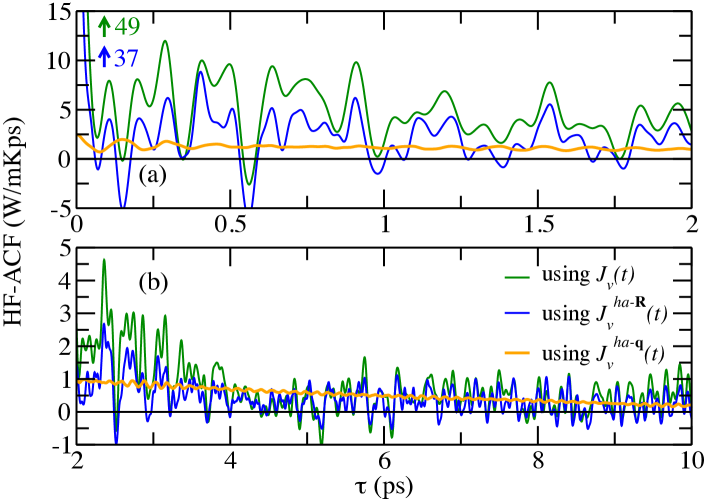
Figure 1: Early (a) and late (b) decay of the heat flux autocorrelation function (HF-ACF) of Silicon computed in a 64 atom supercell with DFT-LDA at a temperature of 960 K (trajectory length $\sim 207$ ps). The green line (${G}[\bm{J}_{v}]$) employs the virial ab initio heat flux $\bm{J}_{v}(t)$ that incorporates all anharmonic effects, whereas the blue and orange lines show the HF-ACFs ${G}[\bm{J}_{v}^{ha}]$ and ${G}[\bm{J}_{v}^{qp}]$ for approximate heat fluxes computed for the exact same trajectory, but imposing the harmonic approximation, i.e., using $\bm{J}_{v}^{ha}(t)$ and $\bm{J}_{v}^{qp}(t)$ defined via Eq. (9) and (10), respectively.

To validate our implementation of the proposed approach in the all-electron, numeric atomic orbital electronic structure code FHI-aims Blum et al. (2009) we compare the heat flux autocorrelation function (HF-ACF) computed from first principles ${G}[\bm{J}_{v}]$ with the respective harmonic HF-ACF ${G}[\bm{J}_{v}^{ha}]$ by evaluating the approximate virial heat flux $\bm{J}_{v}^{ha}(t)$ using the harmonic force constants $\Phi_{IJ}^{\alpha\beta}=\partial^{2}U/\partial{R}_{I}^{\alpha}\partial{R}_{J}^{\beta}$. In the harmonic approximation, the virials

$$\left({\sigma_{I}}^{\alpha\beta}\right)^{ha-\bm{R}}=\frac{1}{2V}\sum_{J\neq I}\Phi_{IJ}^{\alpha\beta}(\Delta{R}_{I}^{\alpha}-\Delta{R}_{J}^{\alpha})({R}_{I}^{\beta}-{R}_{J}^{\beta})$$ (9)

depend only on the positions and displacements from equilibrium $\Delta\bm{R}_{I}=\bm{R}_{I}-\bm{R}_{I}^{eq}$ Ladd et al. (1986), so that $\bm{J}_{v}^{ha}(t)$ can be evaluated using Eq. (6) and (9) along the exact same first-principles trajectory used to compute $\bm{J}_{v}(t)$. As an example, Fig. 1 shows such a comparison: ${G}[\bm{J}_{v}]$ and ${G}[\bm{J}_{v}^{ha}]$ closely resemble each other and become equal for large time-lags $\tau$, which demonstrates the validity of the introduced first-principles definition of the heat flux and its applicability in ab initio GK calculations.

However, Fig. 1 also neatly exemplifies the severe computational challenges of such first-principle GK simulations: Due to the limited time scales accessible in aiMD runs, thermodynamic fluctuations dominate the HF-ACF, which in turn prevents a reliable and numerically stable assessment of the thermal conductivity via Eq. (2). Furthermore, achieving convergence with respect to system size is numerically even more challenging, as classical MD studies based on FFs He et al. (2012); Howell (2012) have shown, so that ab initio GK simulations of solids appear to be computationally prohibitively costly. However, as we will show below, the computational effort can be reduced by several orders of magnitude by a correct extrapolation technique employing a proper interpolation in reciprocal space.

Figure 2: Thermal conductivity ${\kappa}_{\alpha\alpha}$ of Si at 300 and 1000 K computed with the Tersoff-FF. Values extrapolated (left: in time; right graph: in time and size) with our aiGK method are denoted by circles, whereas the dashed lines show the values resulting from a brute force evaluation of ${G}[\bm{J}_{v}]$ using only $\bm{J}_{v}$, i.e., without any extrapolation. 6912 $\bm{q}$-points corresponding to a $12\times 12\times 12$ cubic supercell were used for the size extrapolation in the right plot.

For this purpose, we first note that in the harmonic approximation the HF-ACF can be equivalently Ladd et al. (1986) evaluated in reciprocal space using the heat flux definition in the phonon picture Peierls (1929):

$$\bm{J}_{v}^{ha-\bm{q}}(t)=\frac{1}{2V}\sum_{s\bm{q}}n_{s}(\bm{q},t)\;\omega_{s}^{2}(\bm{q})\;\bm{v}_{s}(\bm{q})\;.$$ (10)

Here, the sum goes over all reciprocal space points $\bm{q}$ commensurate with the chosen supercell; $\omega_{s}(\bm{q})$ are the eigenfrequencies and $\bm{v}_{s}(\bm{q})$ are the group velocities of the phonon mode $s$, which are obtained by Fourier transforming and diagonalizing the mass-scaled force constant matrix $\Phi_{IJ}^{\alpha\beta}$ introduced in Eq. (9). The time-dependent phonon amplitudes and thus the occupation numbers $n_{s}(\bm{q},t)$ can be extracted from the MD trajectory using the techniques described in Ref. McGaughey and Kaviany (2004). Accordingly, we can reformulate the HF-ACF as $\hat{{G}}={G}[\bm{J}_{v}]-{G}[\bm{J}_{v}^{ha-\bm{R}}]+{G}[\bm{J}_{v}^{ha-\bm{q}}]$. For fully time and size converged calculations, $\hat{{G}}$ equals ${G}[\bm{J}_{v}]$; for underconverged calculations (cf. Fig. 1), $\hat{{G}}$ exhibits significantly less thermodynamic fluctuations, since the phases of the individual modes do not enter Eq. (10).

Even more importantly, this formalism enables a straightforward size-extrapolation by extending the sum over (the finite number of commensurate) reciprocal space points $\bm{q}$ in Eq. (10) to a denser grid. The required frequencies $\omega_{s}(\bm{q}^{\prime})$ and group velocities $\bm{v}_{s}(\bm{q}^{\prime})$ can be determined on arbitrary $\bm{q}^{\prime}$-points that are not commensurate with the supercell by Fourier interpolating the force constants $\Phi_{IJ}^{\alpha\beta}$ Parlinski et al. (1997). In the same spirit, we introduce the dimensionless quantity

$$\Delta{n}_{s}(\bm{q},\tilde{t})=\frac{n_{s}(\bm{q},t=\tilde{t}/\omega_{s}(\bm{q}))-\left\langle n_{s}(\bm{q})\right\rangle}{\left\langle n_{s}(\bm{q})\right\rangle}\;,$$ (11)

which accounts for the fact that the equilibrium fluctuations of the occupation numbers are proportional to their equilibrium value $\left\langle n_{s}(\bm{q})\right\rangle={2k_{\mbox{\tiny B}}T}/\omega_{s}^{2}(\bm{q})$ and that the natural time scale $\tilde{t}$ of each mode is determined by its frequency $\omega_{s}(\bm{q})$. As a consequence, we inherently account for the typical $1/\omega^{2}$ dependence of the phonon lifetimes Glassbrenner and Slack (1964); Garg et al. (2011) so that the respective ACFs ${G}[\Delta{n}_{s}(\bm{q},\tilde{t})]$ become comparable and can be accurately interpolated in $\bm{q}$-space (see Suppl. Mat.).

We validate this approach by applying it to FF simulation of Si based on the Tersoff potential, which are known to be particularly challenging to convergence He et al. (2012); Howell (2012). As shown in Fig. 2 for 300 and 1000 K, the proposed interpolation yields remarkable improvements with respect to size- and time-convergence: Panel (a) shows the dependence of $\bm{\kappa}$ on the trajectory length, while panel (b) shows the dependence of $\bm{\kappa}$ on the supercell size. Compared to traditional brute force GK simulations, we achieve reliable values for $\bm{\kappa}$ with sizes as small as 64 atoms and with trajectory lengths as short as 200 ps. This translates into a computational speed-up of more than three orders of magnitude, which in turn enables ab initio Green-Kubo calculations (aiGK) with reasonable numerical effort.

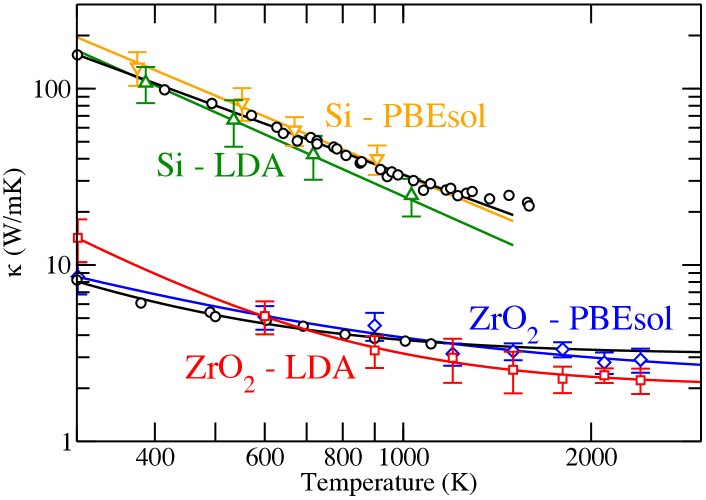
Figure 3: Thermal conductivity ${\kappa}_{\alpha\alpha}$ computed using our aiGK method for Si (LDA green and PBEsol orange triangles) and tetragonal ZrO₂ (LDA: red squares; PBEsol: blue diamonds). Lattice expansion using the quasi-harmonic approximation and the tetragonal-cubic phase transition in ZrO₂ Carbogno et al. (2014) are taken into account. Tabulated values of $\kappa$ are listed in the Suppl. Information. Black circles denote experimental results for single crystals (or extrapolated to this limit) compiled from Ref. Glassbrenner and Slack (1964); Bisson et al. (2000); Youngblood et al. (1988); Raghavan et al. (1998). The lines are generated by fitting the data with ${\kappa}(T)=a+b/T^{c}$.

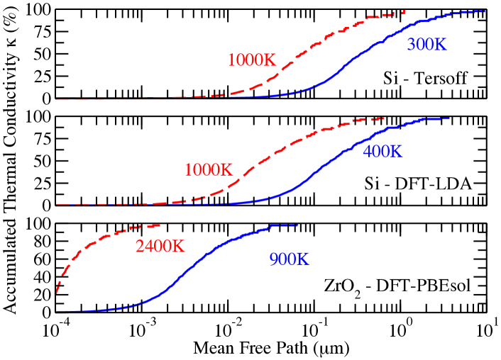
Figure 4: Accumulated thermal conductivity versus mean free path for Si (Tersoff/DFT-LDA) and ZrO₂ (DFT-PBEsol) at different temperatures.

Next, we apply our aiGK technique to compute the temperature-dependent thermal conductivity of Si (64-atom cell) and tetragonal ZrO₂ (96-atom cell) both for the LDA and PBEsol functional. Six trajectories with a duration of 200 ps were used for each data point. In both cases (cf. Fig. 3), we obtain good agreement with experimental data Glassbrenner and Slack (1964); Bisson et al. (2000); Youngblood et al. (1988); Raghavan et al. (1998). For Si, we note that our aiGK extrapolation technique is responsible for up to 50% of $\bm{\kappa}$, especially at low temperatures. Conversely, the thermal conductivities for ZrO₂ are mostly size- and time-converged within the aiMD regime, so that corrections stemming from the extrapolation are always smaller than $10$%. As the accumulated thermal conductivities in Fig. 4 show, the reason for this behavior are the exceptionally low phonon lifetimes or short mean free paths in ZrO₂. Interestingly, we can trace back this behavior to the peculiar, very anharmonic dynamics of zirconia at elevated temperatures. Under such thermodynamic conditions, the oxygen atoms and the lattice tetragonality spontaneously re-orient along a different cartesian direction in a switching mechanism Carbogno et al. (2014). These switches between different local minima of the potential-energy surface constitute a severe violation of the harmonic approximation, given that the dynamics does no longer evolve around one minimum. This is also reflected in the respective dependence on the functional: At the LDA level, the respective barriers are underestimated Carbogno et al. (2014), so that $\bm{\kappa}$ decreases more drastically and at lower temperatures.

In summary, we presented an ab initio implementation of the Green-Kubo method that is applicable for the computation of thermal conductivities in solids, since the proposed unique definition of the heat flux is derived from the virial theorem and based on the local stress tensor. The developed extrapolation technique, which significantly lowers the required computational effort, enables to perform such computations within moderate time- and length scales for the aiMD trajectories. By this means, we are able to accurately compute thermal conductivities for both extremely harmonic and anharmonic materials on the same footing and at arbitrarily high temperatures. In particular, we are able to investigate materials with very low thermal conductivities and high anharmonicities (thermal barriers), for which perturbative treatments relying on the approximate validity of the harmonic approximation would fail. Accordingly, the proposed technique enables for the first time to perform accurate first-principles studies of such materials, which play a pivotal role in a multitude of scientific and technological applications, e.g., as thermal barrier coatings Levi (2004) and thermoelectric elements Snyder and Toberer (2008).