On Primes, Graphs and Cohomology

Abstract.

The counting function on the natural numbers defines a discrete Morse-Smale complex with a cohomology for which topological quantities like Morse indices, Betti numbers or counting functions for critical points of Morse index are explicitly given in number theoretical terms. The Euler characteristic of the Morse filtration is related to the Mertens function, the Poincaré-Hopf indices at critical points correspond to the values of the Moebius function. The Morse inequalities link number theoretical quantities like the prime counting functions relevant for the distribution of primes with cohomological properties of the graphs. The just given picture is a special case of a discrete Morse cohomology equivalent to simplicial cohomology. The special example considered here is a case where the graph is the Barycentric refinement of a finite simple graph.

1. Summary

1.1.

For an integer $n\geq 2$, let $G(n)$ be the graph with vertex set $V_{n}=\{k\;|\;2\leq k\leq n,k\;{\rm square}\;{\rm free}\;\}$ and edges consisting of unordered pairs $(a,b)$ in $V$, where either $a$ divides $b$ or $b$ divides $a$. We see this sequence of graphs as a Morse filtration $G(n)=\{f\leq n\}$, where $f$ is the Morse function $f(n)=n$ on the Barycentric refinement $G$ of the complete graph $P$ on the spectrum of the ring ${\mathbb{Z}}$. The Mertens function $M(n)$ relates by $\chi(G(n))=1-M(n)$ to the Euler characteristic $\chi(G(n))$. By Euler-Poincaré, this allows to express $M(n)$ cohomologically as the sum $\sum_{k=1}^{n}(-1)^{k}b_{k}=1-M(n)$ through Betti numbers $b_{k}$ and interpret the values $-\mu(k)$ of the Möbius function as Poincaré-Hopf indices $i_{f}(x)=1-\chi(S^{-}_{f}(x))$ of the counting function $f(x)=x$. The additional $1$ in the Mertens-Euler relationship appears, because the integer $1$ is not included in the set of critical points. The summation of the Möbius values illustrates a case for the Poincaré-Hopf theorem $\sum_{x}i_{f}(x)=\chi(G(n))$ [5]. The function $f$ is Morse in the sense that in its Morse filtration $G(x)=\{f\leq x\;\}$ the unit sphere $S(x)$ of any integer $x$, which was added last, is a graph theoretical sphere. The Morse index is then $m(x)={\rm dim}(S(x))+1$ and the strong Morse inequalities become elementary in this case.

1.2.

This just summarized story shows that “counting” is a Morse theoretical process, during which more and more ‘handles” in the form of topological balls are added, building an increasingly complex topological structure. When working on the graph $N$ of all natural numbers larger than $1$ with two numbers connected if one divides the other, substantial topological changes happen at square free integers while harmless homotopy deformations take place at the other points. In the homotopically equivalent graph $G$, where only square free vertices are considered, every point is a critical point. The dimension $m(x)$ of the handle formed by adding $x$ defines a Morse index $m(x)\in\{0,1,2\dots\;\}$ satisfying $i_{f}(x)=(-1)^{m(x)}$ and allowing to define $c_{m}(x)$, the number of critical points with index $m$ on $G(x)$. The quantity $c_{0}(x)=\pi(x)+\pi(x/2)$ for example counts the zero-index critical point instances, at which isolated vertices in the form of primes appear and disappear. It relates the prime counting function $\pi(x)$ with a connectedness property of the topological space. As in the continuum, the strong Morse inequalities relate the Betti numbers $b_{k}$ with the counting functions $c_{k}$ of critical points. The zero’th Betti number is $b_{0}(G(x))=1+\pi(x)-\pi(x/2)\leq c_{0}(x)$. For $k>0$ we have $b_{k}(G(x))=\pi(k,x)-\pi(k,x/2)\leq c_{k}(x)=\pi(k,x)+\pi(k,x/2)$, where $\pi(k,x)$ counts the number of prime $k$ tuples whose product is smaller or equal than $x$. The weak Morse inequalities $b_{k}\leq c_{k}$ are trivial, the strong inequalities follow from the exponential decay of $c_{k}(x)-b_{k}(x)=2\pi(k,x/2)$ in $k$.

1.3.

If $n$ is a Kummer number meaning that if $n+1$ is the product of the first $d+1$ rational primes, then the graph $G(n)$ has an involutive time reversal symmetry $k\to(n+1)/k$ which leads to Poincaré duality $b_{k}=b_{d-k}$ for the Betti numbers of the connected component of the graph $G(n+1)$. The connected component of $G(n+1)$ (disregarding the isolated primes) is the Barycentric refinement of $K_{d+1}$, the $d$-dimensional simplex formed on the first $d+1$ primes. We get a discrete version of a Morse-Smale system in which every vertex is a discrete analogue of a hyperbolic critical point whose stable and unstable manifolds behave as if they would intersect transversely. The Morse cohomology on this Morse-Witten complex is equivalent to the cohomology of the graph $P(n)$ which by Kuenneth is equivalent to the cohomology of the Barycentric refinement $G(n)$. There are other connections to number theory. The identity $\sum_{1\neq d|n}\mu(d)=-1$ for example is a manifestation of the fact that a ball has Euler characteristic $1$.

1.4.

This arithmetic example of the natural numbers is a prototype. In full generality, for any suitably defined Morse-Smale function on a finite simple graph, its Morse cohomology is equivalent to simplicial cohomology. While this is not surprising given that the result holds in the continuum, it is crucial to have the right definitions of stable and unstable manifolds at critical points and a correct notion of Morse-Smale in the discrete. It turns out that these definitions can be done for general finite simple graphs regularized by their Barycentric refinement. The set of Morse functions might be pretty limited but if the graph is a $d$-graph meaning that every unit sphere is a (purely graph theoretically defined) $(d-1)$-sphere called Evako sphere, then the notion of Morse-Smale pretty much looks like the one in the continuum: every critical point must have the property that $S^{-}_{f}(x),S^{-}_{-f}(x)$ are spheres and that the corresponding stable and unstable manifolds for two different critical points $x,y$ of index $m,m-1$ intersect transversely or are disjoint. This allows to define an intersection number $n(x,y)$ of two critical points through stable and unstable manifolds and an exterior derivative just like in the continuum. The discrete setup also illustrates why Floer’s generalization to non-orientable and infinite dimensional setups works. We don’t need orientability of the graph in the discrete.

1.5.

Given a finite simple graph $G=(V,E)$. A function $f:V\to\mathbb{R}$ is Morse if it is locally injective and each subgraph of the unit sphere $S(x)$ generated by $S^{-}_{f}(x)=\{y\in S(x)\;|\;f(y)<f(x)\;\}$ is either contractible or a sphere. It is Morse-Smale, if at every vertex $x\in V$, discrete stable and unstable manifolds $W^{\pm}_{f}(x)$ exist which pairwise either do not intersect or intersect transversely in the sense that $W^{-}_{f}(y)\cap S(x)\subset S^{-}_{f}(x)$, allowing to define an intersection number $n(x,y)$ between different critical points: it is $1$ if the orientations agree and $-1$ if the orientations don’t agree. The Morse complex is then defined exactly as in the continuum: the vector space $\Omega(G,f)$ of functions on critical points of $f$ is filtrated by Morse index: $\Omega_{m}(G,f)$ is the set of functions on critical points of Morse index $m$ and admits an exterior derivative $d:\Omega_{m}\to\Omega_{m+1}$ given by $dg(x)=\sum_{y}n(x,y)g(y)$. Morse cohomology is useful, as it is easier to compute as simplicial cohomology. In the discrete, it is also equivalent to Čech cohomology which is the simplicial cohomology of a nerve graph. The Morse function does the job of triangulating the graph.

1.6.

We expect Morse functions in the discrete to be abundant: any injective function $f$ on the vertex set of a geometric graph $G$ should have a natural extension to its Barycentric refinement $G_{1}$, where it is Morse in the sense that adding a new vertex $x$ in the Morse filtration $G(x)=\{f\leq x\;\}$ is either a homotopy deformation or then adds a handle in form of a graph theoretical $k$-ball $B^{-}_{f}(x)$, meaning that the level surface $\{f=c\;\}$ for $c\notin{\rm Ran}(f)$ is always a graph theoretical sphere near the critical point $x$. The case of $f(x)={\rm dim}(x)$ and especially the arithmetic example introduced here illustrates that the graph does not need to have a discrete manifold structure in order for having a discrete Morse theory. In this note, we look only at the special case $f(x)={\rm dim}(x)$ on the Barycentric refinement of a general finite simple graph $G$. It will follow almost from the definitions that in this case, the Morse function $f(x)={\rm dim}(x)$ on the Barycentric refinement $G_{1}$ of $G$ has a Morse cohomology which is identical to the simplicial cohomology of the original graph $G$. Because simplicial cohomology of $G$ is isomorphic to simplicial cohomology of $G_{1}$ of a general statement that Morse cohomology is equivalent to simplicial cohomology. In the continuum this is a well developed theory by Morse, Thom, Milnor, Smale or Floer. For a general theory for finite simple graphs, we need to restrict the Morse functions to a discrete class of Morse-Smale functions and verify that the Morse cohomology obtained is equivalent to simplicial cohomology on the graph. Since as just pointed out, there is always at least one Morse function, we only have still to establish conditions under which deforming $f$ keeps the exterior derivative defined and the corresponding cohomologies unchanged. This will require only the study of local bifurcations of critical points. We plan to work on that elsewhere.

1.7.

Denote by $B^{-}_{f}(x)$ the graph generated by the set of vertices in $S(x)$ for which $f(y)\leq f(x)$ and let $S^{-}_{f}(x)$ the graph generated by vertices in $S(x)$ for which $f(y)<f(x)$. If $S^{-}(x)$ is a discrete sphere so that $\chi(S^{-}(x))$ is either $0$ or $2$, the Morse index $m(x)={\rm dim}(B_{-}f(x))$ at $x$ is defined together by the Poincaré-Hopf index as $i_{f}(x)=(-1)^{m(x)}=1-\chi(S^{-}_{f}(x))$. It measures the change of Euler characteristic when adding the handle $B_{f}^{-}(x)$. The discrete gradient flow defines a Morse-Smale complex whose Thom-Smale-Milnor cohomology is equivalent to simplicial cohomology. In the case of a Barycentric refinement, it is equivalent to the original cohomology of $G$. If $c_{k}$ is the number of critical points of Morse index $k$, and $c(t)=\sum_{k}c_{k}t^{k}$ and $p(t)=\sum_{k}b_{k}t^{k}$ are the Morse and Poincaré polynomials, then the strong Morse inequalities hold: $c(t)-b(t)=(1+t)r(t)$, where $r(t)$ has positive coefficients. In our case this can be shown directly. In general, an adaptation of the semi-classical analysis using Witten deformation [12, 1] is needed. The Witten deformation argument actually shows more: the heat flow of any of the deformed Laplacian $L_{s}$ defined by $f$ not only defines the Hurewicz homomorphism from the fundamental groups to the cohomology groups $H^{k}(G)$, it can be used to match a harmonic form representing a cohomology class with the sphere $S^{-}_{f}(x)$ defined at the critical point $x$ of $f$ as in the limit $s\to\infty$ the support of any harmonic $k$-form is on the union of $k$-spheres associated to critical points.

2. Graphs

2.1.

The natural numbers $\mathbb{N}=\{1,2,3\dots\}$ define a simple graph called the integer graph $N$. Its vertex set is $\mathbb{N}$. The edges are the pairs of distinct integers for which one divides the other. This graph $N$ is simple as we allow no self loops, nor multiple connections. Since $N$ is the unit ball of the integer $1$ and the unit $1$ is not of interest, we better restrict to the unit sphere $S(1)$ of $1$. This graph $S(1)$ in turn is related to a more naturally defined subgraph which we call the prime graph $G$. The vertices of the prime graph $G$ are made of all square free integers in $N$. The graph $G$ can be identified with the Barycentric refinement of the spectrum $P$ of the commutative ring $\mathbb{Z}$, as the vertex set of $G$ is the set of square free integers different from $1$. The spectrum $P$, the set of rational primes is a graph where all vertices are connected to each other. The graph $G$ then generates a sequence of graphs $G(n)$ generated by the vertex set $\{2,3,\dots,n\}\cap\mu^{-1}(\-1,1\})$ of all square free integers smaller or equal to $n$. Similar graphs $G_{R}$ could be constructed from any countable commutative ring $R$: just take the Barycentric refinement of the spectrum of $R$ in which all vertices are connected. On the finite ring $\mathbb{Z}/(n\mathbb{Z})$ for example, the graph would be the Barycentric refinement of the complete graph on the set of all prime factors of $n$.

2.2.

We start with some graph theoretical notations. Given any finite simple graph $G=(V,E)$ with vertex set $V$ and edge set $E$, a complete subgraph $K_{k+1}$ of $G$ with $k+1$ vertices is called a $k$-simplex. The Euler characteristic of $G$ is defined as $\sum_{k=0}(-1)^{k}v_{k}(G)$, where $v_{k}(G)$ is the number of $k$-simplices in $G$. Given a subset $W$ of the vertex set $V$, the graph generated by $W$ is the graph $(W,F)$, where $F$ is the subset of all edges $E$ for which all attached vertices are in $W$. The unit sphere $S(x)$ of a vertex $x$ in $G$ is the graph generated by all the vertices directly connected to $x$. In the graph $N$ for example, the entire graph ring is the unit ball of $1$ with Euler characteristic $1$ and look at the unit sphere $S(1)$. In the graph $G(30)$ for example, the unit sphere of $v=30$ is the cyclic sub graph generated by the vertex set $\{2,6,3,15,5,10\;\}$. In $G(105)$, the unit sphere of the latest added point $v=105$ is a stellated cube, which is a $2$-sphere.

2.3.

Following Evako, graph theoretical spheres are defined by induction [6] first of all, the empty graph $G=(\emptyset,\emptyset)$ is a $(-1)$-sphere. Inductively, for $k\geq 0$, a $k$-graph is a finite simple graph for which every unit sphere is a $(k-1)$-sphere. A $k$-sphere is a $k$-graph which after removing a vertex becomes contractible. A finite simple graph $G=(V,E)$ is contractible, if there exists a vertex $v$ such that both the unit sphere $S(v)$ as well as the graph generated by $V\setminus\{v\}$ are contractible. Two graphs are homotopic if one can get from one to the other by local deformation steps. A deformation step either removes a vertex $v$ with contractible $S(v)$ or adds a new vertex $v$ connected to a contractible subgraph $(W,F)$ of $(V,E)$. All these notions are combinatorially defined without referring to any Euclidean geometric realization. The later would lead to classical topological notions but they are not needed.

2.4.

Given two finite simple graphs $H,G$, the Cartesian product $G\times H$ is defined as the graph whose vertices are the pairs $(x,y)$, where $x$ is a simplex in $G$ and $y$ is a simplex in $H$ and whose edge set consist of all $((a,b),(c,d))$, where either $(a,b)$ is contained in $(c,d)$ or $(c,d)$ is contained in $(a,b)$. This graph product has been ported from simplicial complex constructions to graph theory [7] and has nice properties like that $\chi(H\times G)=\chi(H)\chi(G)$, where $\chi(G)=\sum_{x\subset G}(-1)^{{\rm dim}(x)}$ is the Euler characteristic of $G$ summing over all simplices $x$ in $G$. A special product is $G\times K_{1}$ which is the Barycentric refinement of $G$. Its vertices are the simplices of $G$ and two simplices are connected, if one is contained in the other. The product has all the properties we know from the continuum. It satisfies the Künneth formula for cohomology [7]. It has dimension ${\rm dim}(x)=1+\sum_{x\in V}{\rm dim}(S(x))/|V|$ which satisfies in general the inequality ${\rm dim}(G\times H)\geq{\rm dim}(G)+{\rm dim}(H)$ which is familiar from Hausdorff dimension in metric spaces even so the discrete dimension just defined has no formal relations to Hausdorff dimension in the continuum.

3. Morse theory

3.1.

Lets look at an injective real-valued function $f:V\to\mathbb{R}$ on a countable simple graph $G=(V,E)$ so that we have a filtration $G(n)=\{f\leq n\;\}\subset G(n+1)$ of finite simple subgraphs of $G$. A locally injective function $f$ on the vertex set of a graph $G$ is called a Morse function if for every vertex $x\in V$, the graph $S^{-}_{f}(x)$ generated by the set of vertices $y$ for which $f(y)<f(x)$ is a $m$-sphere for some $m=m(x)\geq-1$. We call $S^{-}_{f}(x)$ the stable sphere of $f$ at $x$. Adding a new prime $p$ for example to the graph $G(p-1)$ produces a critical point for which the unit sphere is the empty graph, and the empty graph is by definition the $(-1)$-sphere. When adding a vertex $x=pq$ with two primes $p,q$ which have not yet been connected anywhere yet, then $x$ is a critical point for which a $0$-sphere has been added. By definition, a $0$-sphere is a $0$-graph (meaning that all unit spheres are $-1$-spheres and that removing one vertex produces a contractible graph, so that a $0$ sphere consists of two isolated discrete points). The Morse index of that added point is then $1$ because the added disc $B(x)$ is a $1$-ball which has a $0$-sphere as its boundary. In the prime graph $G$, this happens for $x=6$ for the first time. If $x=pq$ connects to two primes which are already connected like for $x=15$, where $3-6-2-10-5$ already links $3$ and $5$, we close a loop. We see that adding a new vertex $p_{1}p_{2}\dots,p_{k}$ either destroys a $(k-2)$- sphere or creates a $(k-1)$-sphere.

3.2.

The stable sphere $S^{-}_{f}(x)$ of $f$ at a vertex $x$ can be seen as the intersection of the stable part $\{y\in G\;|\;f(y)<f(x)\;\}$ of the gradient flow of $f$ with the unit sphere in the full graph. Similarly, $S^{-}_{f}(x)$ generated by the vertices in the unit sphere of $x$, where $f(y)>f(x)$ is the unstable sphere. In the case of the prime graph, the stable part of $x$ is just the set of vertices in the graph consisting of numbers dividing the vertex. Remarkably, the stable sphere is always a $m$-sphere for some $m$ allowing to define the Morse index. Given two vertices $x,y$ the heteroclinic connection between $x$ and $y$ is the intersection of the stable and unstable manifolds of $x$ and $y$. The heteroclinic connection between $x=6$ and $y=210$ for example consists of the vertices $\{6,30,42,210\;\}$.

3.3.

Since every vertex is a critical point, there is no discrete gradient flow on the graph itself, at least when trying to define it as in the traditional sense. The reason is that every point would be a stationary point. We still can think of the stable parts and unstable parts of the unit spheres as part of “stable and unstable manifolds”. It would be possible to get a classical gradient flow by doing a geometric realization of the simplicial complex and then define a gradient flow on that manifolds. The easiest would be to embed $G(x)$ in $R^{n}$ if $x$ is a product of $n$ primes and map every point $y=p_{0}\dots p_{k}$ to a point $x$ for which $x_{p_{j}}=1$ for every $0\leq j\leq k$ and $0$ else. Then define a suitable function $f(x)$ which embeds the discrete geometry into the continuum. Doing so would be inelegant as finite combinatorial problems should be dealt using finite sets.

3.4.

A first observation which led us to write this note down is the realization that the counting function $f(x)=x$ is a Morse function on the prime graph $G$: its Morse filtration is homotopic to the Morse filtration of the integer graph $S(1)\subset N$ and the Euler characteristic is related the Mertens function $M(x)=\sum_{k=1}^{n}\mu(k)$ by the formula $\chi(G(x))=1-M(x)$. The Poincaré-Hopf index $i_{f}(x)=1-\chi(S^{-}_{f}(x))$, is the Möbius function $\mu(x)$ which is $1$ if $x$ is a product of an even number of distinct primes and $-1$ if $x$ is a product of an odd number of distinct primes and $0$ if there exists a square factor different from $1$ in $x$. At points, where $\mu(x)=0$, the graph extension $G(x-1)\to G(x)$ is a homotopy deformation step, during which no interesting topology changes happens. When restricting to the graph $G(n)$ whose vertices are the square-free integers $\leq n$, every vertex in the graph is a critical point. The formula $\chi(G(x))=1-M(x)$ can be seen as the Poincaré-Hopf formula, where the indices are $-\mu(x)$ and the Mertens function includes the index $1$ of the point $1$, which we do not consider. Note that the integer graph $N=B(1)$ for which the vertex set is $\mathbb{N}$ has Euler characteristic $\chi(N)=1$ as it is the unit ball of a vertex.

3.5.

At critical points $x$ of $f$, where $x$ gets attached to a sphere $S^{-}_{f}(x)$ with Euler characteristic $0$ or $2$, the Poincaré-Hopf index is $i_{f}(x)=\pm 1$. If $B_{f}^{-}(x)$ is the graph generated by $x$ and $S^{-}(x)$, then the dimension $m=m(x)$ of the stable ball $B_{f}^{-}(x)$ is called the Morse index of $x$. For a Morse function $f$ on a finite simple graph, denote by $c_{m}(f,G)$, the number of critical points with Morse index $m$. In the case $G(x)$, we simply write $c_{m}(x)$. The Morse counting functions $c_{m}(f,G)$ are of interest: for the Morse function $f(x)=x$ on the integer graph $G$ or prime graph $P$, we have $c_{0}(x)=\pi(x)+\pi(x/2)$ with prime counting function, as every prime $p\leq x$ is a critical point with Morse index $0$ (the handle $\{x\}$ with $-1$ dimensional unit sphere $\emptyset$ has been added) and every number $2p\leq x$ is a critical point with Morse index $1$ (the $1$-ball $\{2,p,2p\}$ with 0-dimensional unit sphere $\{2,p\}$ was added). As the prime counting function, also the functions $c_{k}(x)$ for larger $k$ could be interesting. To make them accessible by Morse theory, we need cohomology.

4. Cohomology

4.1.

Given a finite simple graph like $G(x)$, we can assign an orientation to its maximal simplices. This does not need to be an orientation of the entire graph as we don’t require the orientations to be compatible on intersections of two simplices. The choice of the orientations will not matter. It corresponds to a choice of basis in a vector space. Cohomology is by Hodge a spectral notion which does not depend on the choice of this basis: the groups are the kernels of Laplacians which are orientation independent. Let $\Omega^{k}(G)$ denote the set of functions on $k$-simplices such that changing the orientation of a simplex $x$ changes the sign of $f$. These are discrete $k$-forms. Define the exterior derivative as $df(x)=f(dx)$, where $dx$ is the boundary chain of $x$. Since the boundary operation $d$ satisfies $d^{2}x=0$, the exterior derivative operation satisfies $d^{2}f=0$. The $k$’th cohomology group $H^{k}(G)$ is defined as ${\bf ker}(d|\Omega^{k})/{\bf im}(d|\Omega^{k-1})$. The Hodge Laplacian $L=(d+d^{*})^{2}$ is a $v\times v$ matrix with $v=\sum_{i=0}^{\infty}v_{i}$. It splits into blocks $L_{k}$. The dimension $b_{k}(G)$ of the vector space $H^{k}(G)$ is called the $k$’th Betti number of $G$. By Hodge theory, $b_{k}(G)$ is the nullity of the matrix $L_{k}$. For example, $b_{0}(G)$ is the number of connected components of $G$.

4.2.

By the Euler-Poincaré formula, we can now write $\chi(G(x))=\sum_{k=0}^{\infty}(-1)^{k}b_{k}(x)$ with Betti numbers $b_{k}(G)$. Since we have a finite graph, this sum is finite. We see that the Mertens function has a cohomological interpretation. and that the Morse index $m(x)$ which gives the dimension of the attached or removed handle satisfies $-\mu(x)=i_{f}(x)=(-1)^{m)}=(b_{m}(x)-b_{m}(x-1))$. More number theoretical functions which relate to cohomology through Morse theory are obtained by counting critical points. We look at them next.

4.3.

The number $c_{m}(x)$ of critical points for which $S^{-}_{f}(x)$ has dimension $m-1$ satisfies the Morse inequalities $(-1)^{p}\sum_{k\leq p}(-1)^{k}[c_{k}-b_{k}]\geq 0$ or $(-1)^{p}\sum_{k>p}(-1)^{k}[c_{k}-b_{k}]\leq 0$. The two just given statements are equivalent since the Euler-Poincaré identity reads $\sum_{k=0}(-1)^{k}[c_{k}-b_{k}]=0$. Witten’s idea using the deformed derivative $e^{-sf}de^{sf}$ would give even more information using semi-classical analysis. The Morse counting functions $c_{k}(G)$ are of some interest, as $c_{0}(x)$ grows like the prime counting function $\pi(x)$. The function $c_{1}(x)$ related to closed loops grows at least like the prime triple counting function $\pi_{3}(x)$ counting the number of triples $p,q,r$ of primes with $pqr\leq x$. More precisely, $c_{1}(x)\geq|\{(p<q<r)\;|\;qr\leq x,pqr>x\;\}|$ $+|\{(p<q<r)\;|\;pqr\leq x\;\}|$ which counts instances where circles $p,pq,q,qr,r,rp$ were “born” plus the number of discs $p,pq,q,qr,r,rp,pqr$ which are burial grounds, where circles have ”died”. The weak Morse inequalities $b_{k}\leq c_{k}$ already lead to $\sum_{k=0}^{n}b_{k}\leq\pi^{2}n/6$.

4.4.

Counting is a dramatic process which tells the story of the life and death of spheres. While we can only look at the events, where a square free number is added, we can also look at the full story. For $n=1$, space is the empty graph. At $2,3$, new $0$-balls are added. At $n=4$ nothing interesting happens, as the longly $2$ forming a graph $K_{1}$ gets a homotopy deformation to a $K_{2}$. At $n=5$ another $0$-sphere is added. At $n=6$, we see the creation of a $1$-ball and a destruction of the $0$-sphere $\{2,3\}$. At $n=7$ an other $1$-ball is added. At times $n=8$ and $n=9$, nothing spectacular takes place as we observe just homotopy deformations. At time $n=10$, a $1$-ball gets glued to the sphere $\{2,5\}$. The first 1-sphere is born at $n=15$. This circle dies at $n=30$. The first 2-sphere sees the light at $n=105=3*5*7$ and dies at $n=210=2*3*5*7$. The unit sphere of a new square-free vertex $n$ is always a sphere $S_{f}(x)$ and the change of Euler characteristic is the index $i_{f}(x)=1-\chi(S_{f}(x))$. When adding $x$, the ball $B_{f}(x)$ is the handle which gets attached to the sphere $S_{f}(x)$. It either destroys the sphere $S_{f}(x)$ and adds a new sphere.

4.5.

The Betti numbers $b_{k}(G(x))$ reflect on essential parts of the geometry and so report on more interesting feature of the topology of the graph $G(x)$. Classically, Betti numbers were estimated by other means, especially in terms of curvature and diameter. While we don’t pursue this here, the prime graphs give us a source of examples of graphs, where we can compute all cohomologies without actually computing the vector spaces from exterior derivative explicitly and where arbitrary high Betti numbers matter. One can speculate that some work on curvature estimates could eventually shed some light on the Riemann hypothesis. But certainly this does not happen on the elementary level we treat the topic here. We look at things the opposite way: we have a source of examples of graphs, where we can compute arbitrary high cohomology groups by other means. We have computed the cohomology groups up to $n=250$ the hard way explicitly using Hodge by computing the kernels of the Laplacians. It could be possible that the actual representatives of the cohomology groups, the harmonic forms, vectors in the kernel of $L_{k}$ are of number theoretical interest. Also still unexplored spectral properties of the form-Laplacians $L_{k}$ could be of number theoretical interest.

5. More remarks

5.1.

It is more natural to use the ring $\mathbb{Z}$ of integers rather than the semi-ring $\mathbb{N}$ of natural numbers. The spectrum $P$ of $\mathbb{Z}$ is the set of prime ideals in $\mathbb{Z}$ which naturally can be identified with the set of prime numbers. An abstract simplicial complex on $P$ is given by the collection $K$ of all finite non-empty subsets of $P$. It is the Whitney complex of the complete graph defined on $P$. The Barycentric refinement of the complex $K$ is the Whitney complex of the graph for which the vertices are the square free positive integers different from $1$ and where two integers are connected, if one is a divisor of the other. As described in the introduction, we call this the prime graph.

5.2.

Here is a bit more mundane approach which motivates to look at square free integers: consider the finite set $P_{n}$ of primes in $I_{n}=\{2,\dots,n\;\}$. The set of all subsets of $P_{n}$ for which the product is in $I_{n}$ is still a simplicial complex even so it is not a Whitney complex of a graph. However, its Barycentric refinement $K$ is the Whitney complex of a finite simple graph $G(n)=(V(n),E(n))$ which we call the Morse filtration of the prime graph: the vertices $V(n)$ are the set of square free numbers in $I_{n}$ and two vertices are connected if one is a divisor of the other. the prime numbers are the atomic points and the division structure equips $V(n)$ with a partial order structure. The integer $35$ for example contributes to the sets $\{3\},\{5\},\{3,5\}$ to $K$ It can be seen as a ”line segment” as the intersecting ideal $[5\times 7]$ which connects the ideals $[5]$ and $[7]$. More generally, any square-free integer $x=p_{1}p_{2}\cdots p_{k}$ defines a $(k-1)$-dimensional simplex or faces in $K$. It becomes a point in the prime graph $P$ containing the finite graphs $G(n)$. The Möbius function $\mu(x)$ which originally assigns to a simplex $x$ of dimension $k$ the valuation $\mu(x)=(-1)^{k}$ is now a function on the vertices of $G(n)$ and it is the Poincaré-Hopf index $i_{f}(x)$ of the counting function $f$.

5.3.

The Euler characteristic $\chi(G(n))$ of the prime graph is now equal to $1-M(n)$ as $1$ does not belong to the spectrum of $Z$. Geometrically speaking, $G(n)$ is a subgraph of the unit sphere of $1$ in $G(n)$. The entire integer graph $G(n)$ is a homotopy extension of the unit ball of $1$. Since the $k$-simplices in the unit ball of $1$ belong to $(k-1)$-simplices in the unit sphere we get a sign change in $\chi$ and a shift in the dimension of cohomology for $k\geq 1$. Because nothing interesting happens at points $x$ which are a multiple of a square prime, the Barycentric refinement $G(n)$ of the spectral simplicial complex is equivalent to the integer graph $G(n)$. Actually, including a vertex $n$ which contains a square larger than $1$ would produce a homotopy deformation of the graph and not change the Euler characteristic. For example, removing $9$ from $G(12)$ does not change its topology as the unit sphere of $9$ is the contractible set $\{3\}$. We stick with the prime graphs $G(n)$ containing $Q(x)$ vertices rather the graphs $G(n)$ with vertex set $\{1,\dots,n\}$. Since the Basel problem renders $Q(x)$ proportional to $x$ with proportionality factor $\pi^{2}/6$, not much is gained from this homotopy reduction, but it helps for visualization purposes to discard the homotopically irrelevant parts. Figure (1) visually illustrates this.

5.4.

Euclid saw “points” as ‘that which has no part”, line segments as a connection between two points and “triangles” as a geometric objects defined by three points. The graph $G(n)$ is a geometric object containing points, line segments, triangles and higher dimensional simplices, where the geometrically defined quantity $\chi(G(n))$ is of number theoretical interest. The Mertens function is a determinant of the Redheffer matrix and now also cohomologically expressible as kernels of matrices. The Moebius function $\mu(x)$ is the Poincaré Hopf index of the scalar Morse function $f(x)=x$. If the $k$’th Betti number changes, we add a $k$-dimensional handle. For each $n$, the trivial weak Morse inequalities $b_{p}\leq c_{p}$ generalize to the statement that $c(t)-b(t)=(1+t)R(t)$ where $R(t)=\sum_{k}r_{k}t^{k}$ satisfies $r_{k}\geq 0$. The weak Morse inequalities compare the coefficients of $c-b$ the strong Morse inequalities are obtained by comparing the $t^{p}$ coefficients of $\sum_{k}r_{k}t^{k}=(\sum c_{k}t^{k}-\sum b_{k}t^{k})(1-t+t^{2}\dots)$.

5.5.

The graph $G(n)$ can contain ”dust” in the form of isolated vertices. These zero-dimensional part consists of primes in $(n/2,n]$ not yet attached to the main graph. Then there are ”hairs”, which are line segments $p,pq,q$ of primes $p,q$, where $q$ is not connected to any other prime. Then there are basic ”loops” $p,pq,q,qr,r,rp$ with triples of primes, where none of the composite numbers are connected to anything else. Two dimensional ”disks” are obtained by triples of primes like that but with an additional central vertex $rpq$. Increasing $n$ reaching such a vertex is an example where we add a two dimensional handle. The first embedded 2-sphere only appears for $n=105=3*5*7$. Only at $n=1155=3*5*7*11$, the first $3$-sphere is present in $G(n)$.

5.6.

If $n$ is the Kummer number $n=2\cdot 3\cdot\dots\cdot p-1$, which is one less than the product of the first $k$ primes, then the graph $G(n)$ has counting as a Morse-Smale system. The reason is that we have then a time reversal involution $k\to(n+1)/k$ on $G(n)$. While in general, the graphs $G(n)$ have a trivial automorphism group, in the case of the Kummer number, we have an involution. Now, we not only have the stable manifold of a vertex but also an unstable one. Every vertex $v$ is a hyperbolic critical point. The stable sphere $S^{-}_{f}(x)$ can be seen as the analogue of defining the stable manifold. Due to time reversal, we also have an unstable sphere $S^{+}_{f}(x)$ as part of the unstable manifold. Now given two vertices $x,y$ in $G(n)$, since both are critical points, we can look at the connecting manifold which can be empty. For example, in $P(209)$, we can connect the two vertices $2$ and and $70$ via the homoclinic connection $2,10,70$. We have now what one calls a Morse-Smale system.

6. Illustrations

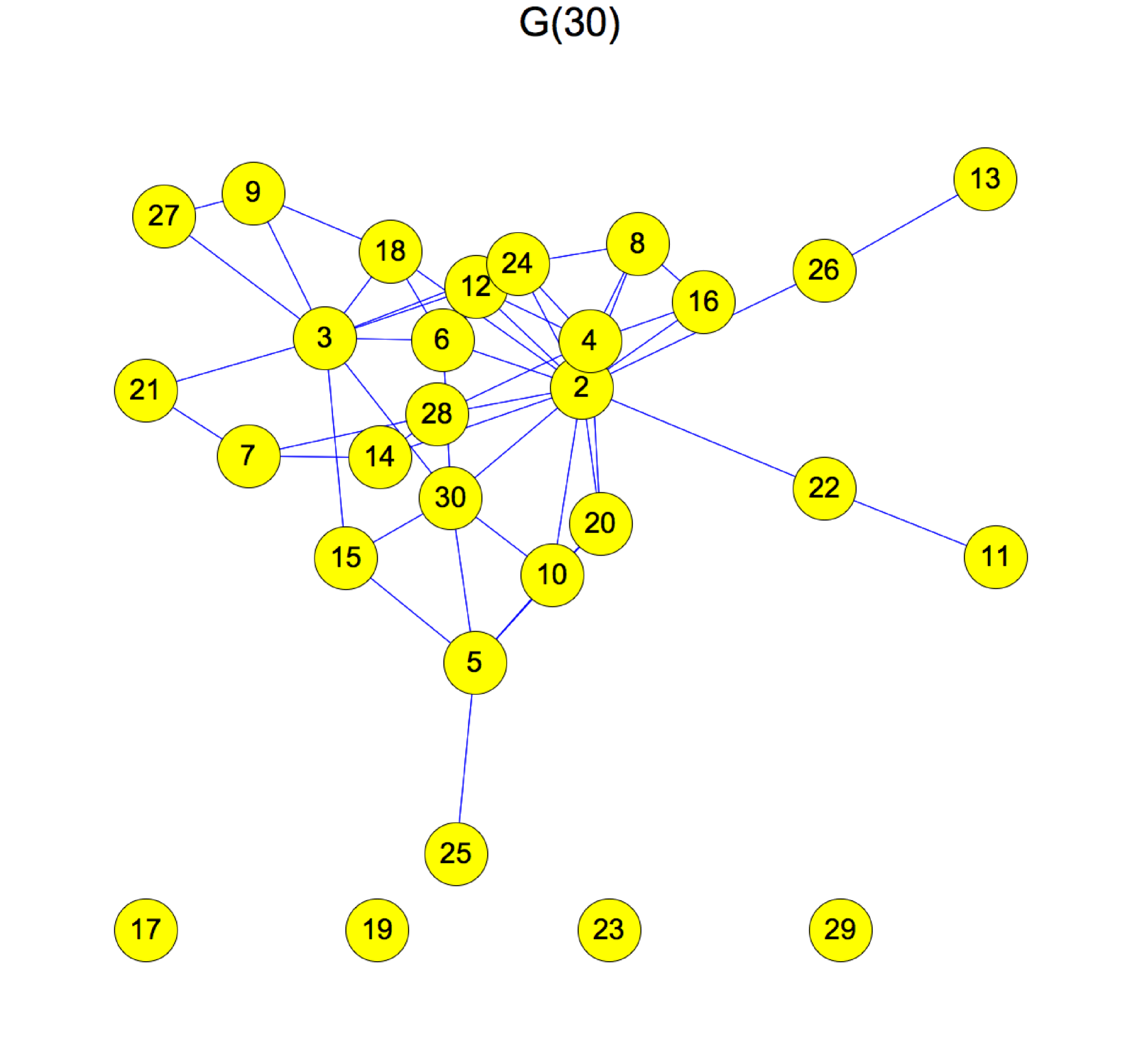
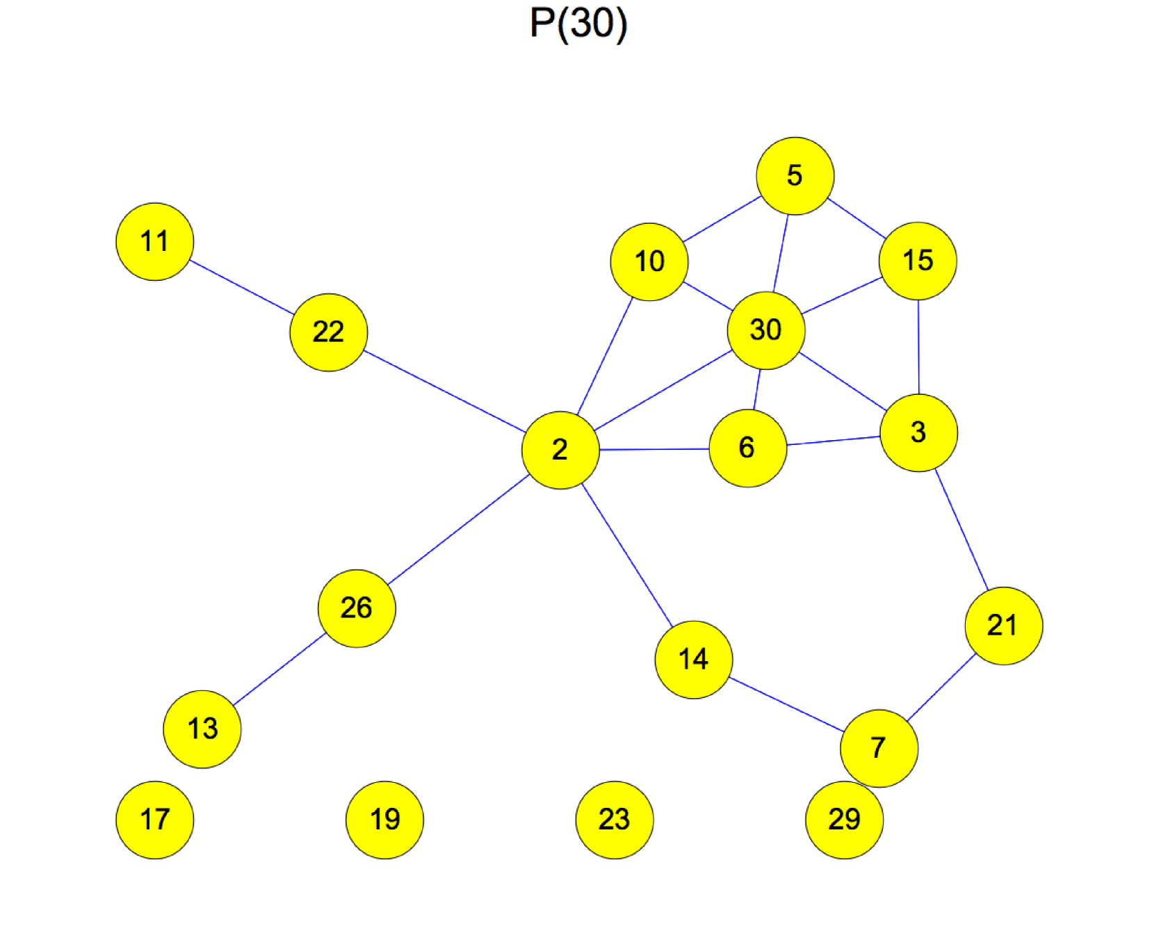
Figure 1. The integer graph $G(30)$ contains irrelevant parts like the $3$-simplex $2,4,8,16$ and is the unit ball $B(1)$ of $1$. As a ball it always has Euler characteristic $1$. Removing $1$ gives the unit sphere $S(1)$ which after removing the homotopically irrelevant parts gives the prime graph $P(30)$ which is a Morse cut of the Morse function $f(x)=x$ on the Barycentric refinement $P$ of the complete graph on the spectrum of the ring of integers $Z$. It is homotopic to $S(G(n))$ and has shifted cohomology and satisfies $b_{0}(P(n))=H^{0}(P(n))=\pi(n)$, the prime counting function. The 2-disk $B(3)$ in $P(30)$ has been added when the point $2\cdot 3\cdot 5$ was joined. It decreased the Betti number $b_{1}$ by $1$. The prime graphs $P(n)$ are not only simpler, they are also more naturally defined as the Barycentric refinement of the spectrum of the commutative ring $Z$ rather than a semi ring $N$ like the integer graphs $G(n)$. The fact that the cohomologies agree is a special case of the fact that Morse cohomology is equivalent to graph cohomology.

Figure 2. In this figure we see first the integer graph containing all integers $2,\dots,19$ as vertex set. As before, the unit $1$ is removed so that we only see the unit sphere of $1$. The graph is homotopic to the prime graph $G(19)$ seen to the right. which only contains the square free integers. These integers are critical points of the counting function $f(x)=x$ which has the Möbius function $\mu(x)$ as Poincaré-Hopf index. The fact that the Möbius function is zero on integers containing a square of a prime reflects the fact that when adding such a vertex nothing interesting happens topologically: adding such a vertex is a homotopy deformation similarly as in topology where a change of the value $c$ of a Morse function does not change the homotopy of $\{f\leq c\}$.

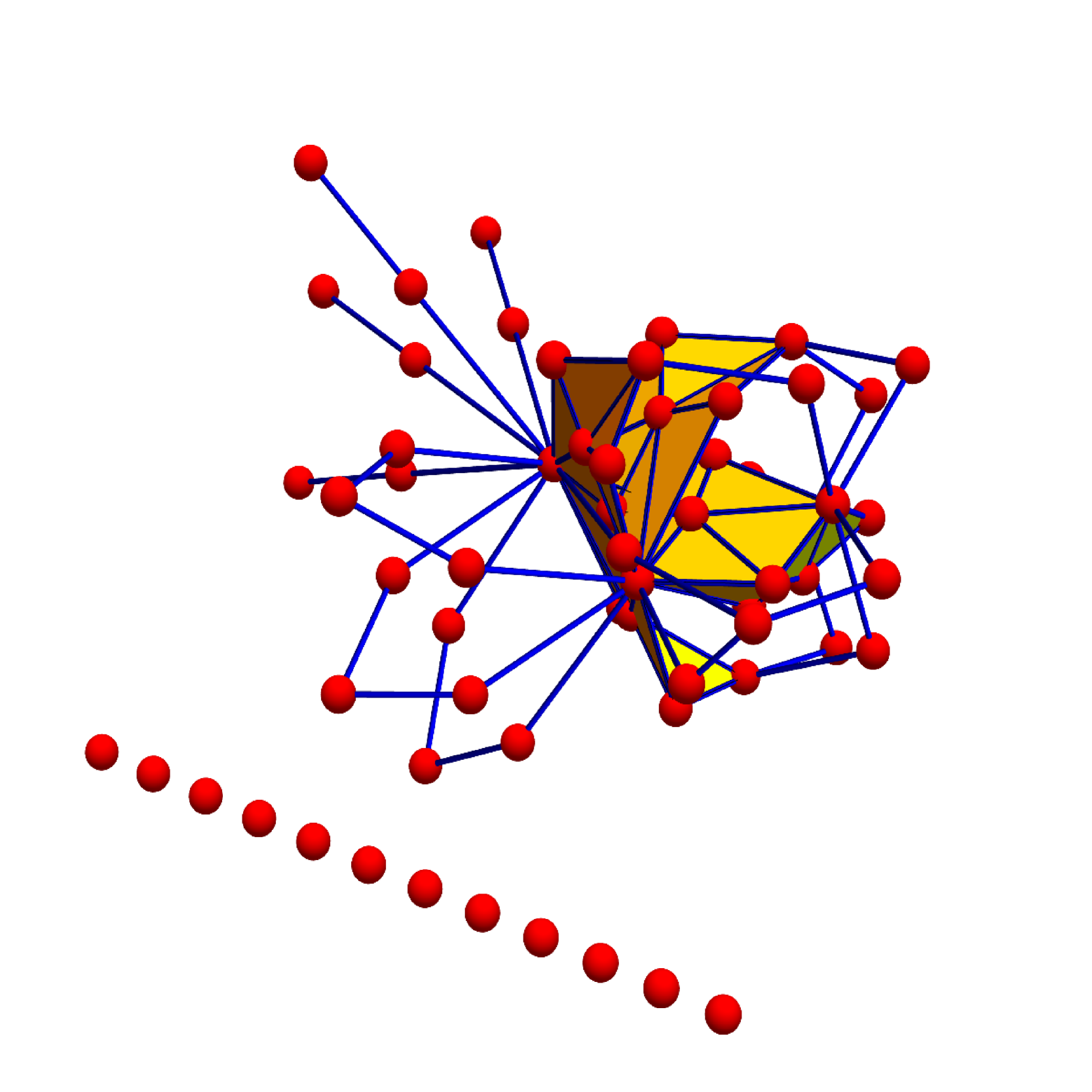
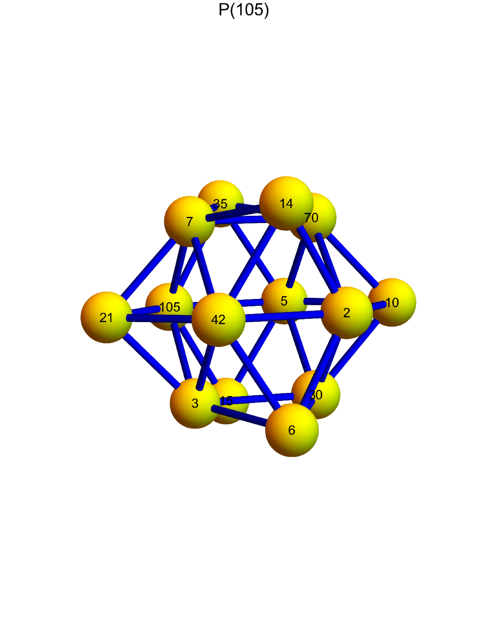
Figure 3. The prime graph $G(105)$ is the smallest $G(n)$ containing a $2$-sphere contributing to a positive $b_{2}$. Its sphere is $S(210)$ in $G(210)$ is seen to the right and is defined by the 4 primes $2,3,5,7$. It is a stellated cube. The number $105$ is the smallest integer for which we have a vertex with Morse index $m(x)=2$. This sphere stops to matter topologically again when the point $210=2\cdot 3\cdot 5\cdot 7$ is added, which produces a central vertex, adding a 3-dimensional handle. For any quadruple $p_{1}<p_{2}<p_{3},p_{4}$ of primes, the sphere appears for $x=p_{2}p_{3}p_{4}$ and disappears at $x=p_{1}p_{2}p_{3}p_{4}$. It illustrates how the Morse counting function $c_{k}(x)$ are number theoretical.

Figure 4. The dimension of a graph is inductively defined as ${\rm dim}(G)=1+\sum_{x\in V}{\rm dim}(S(x))/|V|$. We see the graph of numerically computed dimensions of $G(n)$ for $6\leq n\leq 2690$. The best fit with the functions $1,x,\log(x)$ is $0.0764206-0.0000483082x+0.195795\log(x)$. The growth of the dimension is related to the growth rate of primes but the link has not yet been established.

Figure 5. The Wu characteristic $\omega(G)$ and an affinely scaled Euler characteristic $100-15*\chi(G)$ of the prime graphs $G(n)$ for $n\leq 259$. We initially constructed the prime graphs $G(n)$ as example graphs to investigate the Wu characteristic.

7. More Remarks

7.1.

$b_{0}$ increases if $x=p$ is a prime and decreases if it is connected to the main connected component which happens if $x=2p$. $b_{1}$ increases if $x=p_{2}p_{3}$ for $p_{1}<p_{2}<p_{3}$ and decreases if $x=p_{1}p_{2}p_{3}$. $b_{2}$ increases if $x=p_{2}p_{3}p_{4}$ for $p_{1}<p_{2}<p_{3}<p_{4}$ and decreases if $x=p_{1}p_{2}p_{3}p_{4}$. The Betti number $b_{3}$ increases for $x=p_{2}p_{3}p_{4}p_{5}$ and decreases again if $x=p_{1}p_{2}p_{3}p_{4}p_{5}$.

7.2.

We have seen that the natural numbers $N$ define a geometric object $P$ for which the asymptotic of the Mertens function provides a limiting Euler characteristic of a Morse filtration. This limit is not a number but an asymptotic. Famously and popularized since more than a century, knowing the limiting growth rate of $M(n)$ would settle the Riemann hypothesis RH. We see now that RH has a topological component. A pioneer of studying this question, Franz Mertens, was also the calculus teacher of Erwin Schroedinger. It was probably realized long before Mertens that an estimate $M(n)\leq n^{1/2+\epsilon}$ for all $n$ would imply $1/\zeta(s)$ to be analytic in $Re(s)>1/2+\epsilon$. as the Riemann functional equation implies then the roots of $\zeta$ are then away from the strip $[1/2-\epsilon,1/2+\epsilon]$.

7.3.

Feller [2] illustrated the popular Mertens reformulation of the RH in a probabilistic way: if the Möbius function $\mu(n)$ were sufficiently random, then by the law of iterated logarithms the estimate $M(n)\leq\sqrt{n\log\log(n)}$ would hold. Already Stieljes, in 1885, showed interest in the Mertens function in relation to the Riemann hypothesis. The probabilistic intuition supports the believe that RH is reasonable and also explains why the initial conjecture of Mertens (which was already conjectured in a letter from Stieljes to Hermite) that $M(n)\leq\sqrt{n}$ is too strong. Indeed, Odlyzko and te Riele [9] disproved it thirty years ago. While it is still not known whether $M(n)/\sqrt{n}$ is bounded, the probabilistic heuristic of Feller of the iterated log theorem makes it likely that $M(n)/\sqrt{n}$ indeed will grow like $\log(\log(n))$. According to [9] also a conjecture by Good and Churchhouse asking whether $\limsup M(n)(x\log(\log(x)))^{-1/2}=\sqrt{12}/\pi$ appears too optimistic.

7.4.

The free Riemann gas or primon gas model [11] gives to a vertex $p$ in the set of primes the energy $\log(p)$. Since the energy of a simplex $n=p_{1}\dots p_{k}$ is $E(n)=\log(n)$, it defines an energy on the Barycentric refinement, which in this model leads to the second quantized Hamiltonian. It is the Pauli inclusion principle which leads to the graph $G$. The function $\mu(n)=(-1)^{k}$ is the Fermion operator. It is positive for bosons, negative for fermions. While without exclusion principle, the partition function of the model at inverse temperature $s=1/T$ is $\sum_{n}e^{-E(n)/T}=\sum_{n}e^{-\log(n)s}=\sum_{n}1/n^{s}=\zeta(s)$, the partition function with Fermion statistics is the Dirichlet character $\sum_{n}\mu(n)e^{-\log(n)s}=\sum_{n}\mu(n)/n^{s}=1/\zeta(s)$. In this model, the Riemann hypothesis is a statement about the partition function. The pole at $s=1$ is the Hagedorn temperature.

7.5.

In the continuum, there are estimates of Gromov [4] of the type $b_{k}\leq C^{1+\kappa D}$ where $D$ is the diameter $-\kappa$ the minimal sectional curvature of the manifold. For graphs $G(n)$ we indeed have an estimate $\kappa D\leq\log(n)/\log\log(n)$ which is better than the Gromov estimate but still not strong enough to prove RH. Constants are important and as expected, topology alone is hardly the silver bullet. Still, topology motivates to look at discrete differential geometric notions like curvature and its connection to Betti numbers in general. Indeed it provokes the question whether in full generality, for any finite simple graph, a Gromov type estimate $b_{k}(G)\leq e^{c_{k}\kappa(G)d(G)}$ holds for finite simple graphs, where kappa is the minimal sectional curvature and $d(G)$ the diameter of the graph.

7.6.

We first we have to define the minimal sectional curvature $\kappa$ for a finite simple graph. Let $\kappa$ be the maximum for which the sectional curvature satisfies $1-{\rm deg}_{W}(x)/6\geq-\kappa$ for all vertices $x$ and wheel sub graphs $W$. For $G(n)$, the curvature is bounded by $1-\nu(n)/3$, where $\nu(n)$ is the maximal number of distinct prime factors of $n$. We know $\nu_{n}\leq\log(n)/\log\log(n)$.

7.7.

The diameter of the graph $G(n)$ is bounded above by $5$. Proof: take two vertices $k,m$. If both are not prime they both have a smaller factor $p,q$. The path $k,p,2q,2,2q,q,m$ shows that $d(k,m)\leq 6$ because all numbers $p,2q,2,2q,q$ are smaller or equal than $n$ so that this path is in $G(n)$. The distance is even $\leq 4$ then as if $p$ is the smallest prime factor of $k$ and $q$ the smallest of $m$, then $pq\leq\sqrt{km}\leq max(m,n)$ so that $k,p,pq,q,m$ is in $G(n)$ and $d(k,m)\leq 4$. If $k,m$ have a common prime factor $p$, then their distance is even $2$ as the path $k,p,m$ shows. If $k=p$ is prime but connected to the main component, then there is a point $pl\leq n$ so that $2p\leq n$. The path $p,2p,2$ is in $G(n)$ meaning $d(p,2)\leq 2$. We see that for any integer $m$, $d(m,2)\leq 3$. This shows that the distance in that case is $\leq 5$ with connection $p,2p,2,2q,q,m$ of length $m$. If both $n,m$ are prime their distance is $\leq 4$. All graphs $G(n)$ with $n\geq 15$ have diameter $5$ where the maximal distance is obtained between a prime $p$ and a composite number $m=qr$ with shortest connection $p,2p,2,2q,q,m$ which can not be shortened. For the graph $G(15)$ it is the distance between $11$ and $15$ as $11,22,2,10,5,15$ and $11,22,2,6,3,15$ are the two shortest paths from $11$ to $15$.

7.8.

In our case, the Gromov formula gives a bound on the Betti numbers $C^{5\log(n)/\log\log(n)}$ which is only polynomial in $n$. Using the simplest Morse inequality $b_{k}(G(n))\leq c_{k}(G(n))$ we can see better as $c_{k}$ grows like the number $\pi_{k}(n)$ telling how many prime $k+1$-tuples $p_{0}<p_{1}<p_{2}<\dots<p_{k}\leq n$ there are. Neglecting constants we have $c_{k}\leq n^{k}/(\log(n)^{k}k!)$. The Morse inequalities now gives us information about the alternating sum $\sum_{k}(-1)^{k}c_{k}$ in terms of the growth of the Mertens function. We see this here reflected a relation between the prime number distribution and the growth of the Mertens function related to the Euler golden key $\sum_{n}\mu(n)/n^{s}=1/\zeta(s)=\prod_{k}(1-1/p_{k}^{s})$.

7.9.

We initially have used the graphs $G(n)$ as a play ground to investigate the Wu characteristic $\sum_{x\sim y}(-1)^{{\rm dim}(x)+{\rm dim}(y)}$ summing over all pairs of interacting simplices $x,y$ (see [8]). This number is like Euler characteristic a functional on graphs which is multiplicative and satisfies Gauss-Bonnet or Poincaré-Hopf formulas. It is natural to ask whether the growth rate of $\omega(G(n))$ has any relation to analytic properties of some zeta function.

7.10.

Geometry enters basic counting principles. Geometric arrangements of pebbles on rectangular patterns motivated on a fundamental level to accept commutativity laws $n\times m=m\times n$ despite that on a fundamental level, nature does not multiply commutatively as the Heisenberg anti-commutation relation $pq-qp=\hbar$ shows. Neglecting square parts is not only important in combinatorics it is also the reason for fundamental principles like Pauli exclusion. In our geometric picture, adding numbers with square factors is a homotopy which does not change Euler characteristic. It is the Fermionic nature of calculus which fundamentally evaluates on oriented substructures and changes sign when the orientation is switched. With a number like 12, switching two prime factors 2 would change the sign but not the number. It is the interpretation of numbers as simplices in a simplicial complex which makes this clear.

7.11.

Our understanding of what a ”point” is has changed over time: while the first mathematicians saw points as marks or pebbles without formal definition, it was Euclid who first saw the need to define it. He decided to declare a points to be something ”that which has no part”. Descartes started to access points through algebra. This has been evolved more and more since. Points are now seen as maximal ideals in a commutative ring. In analysis, the Gelfand representation theorem identifies points of a $C^{*}$ algebra as elements in the spectrum. The Nullstellensatz identifies points of an affine variety as maximal ideals of the ring its regular functions. While already Kummer and Noether saw prime ideals as generalized points, irreducible varieties like an elliptic curve $y^{2}=x^{2}+x+1$ are now seen as ”points” in a ”spectrum” on which Zariski built a topology in which closed sets are the set of prime ideals which contain a fixed prime ideal. Grothendieck took the picture that prime ideals are points more seriously even so he considered the notion of a ”scheme” as a setup of ”infantile simplicity”. But it is the simplicity which makes it appealing. The ring of integers as the simplest scheme has been studied since the very beginning of mathematics.

7.12.

An partial order structure given by an abstract simplicial complex can not be visualized well. Fortunately, after a Barycentric subdivision, any abstract finite simplicial complex is the Whitney complex of a finite simple graph. Graphs are more intuitive as they can be drawn in such a way that the vertices and edges alone determine all the topological information of the original simplicial complex. Its cohomology or Euler characteristic for example is the same. The graph category also comes naturally with analytic structures like incidence matrices and Laplacians. However, restricting to graphs is merely language as the Barycentric refinement of any simplicial complex is already the Whitney complex of a graph. It is useful language however as it is a basic data structure known to many computer languages.

7.13.

For a ring in which the unique factorization fails, the Morse condition can fail. A case, where things still work is the ring of Gaussian integers. There is a canonical counting function as we can only primes in equivalence classes. This means, we look at primes in the quotient $\mathbb{C}/D_{4}$, where $D_{4}$ is the dihedral group generated by the units in $\mathbb{C}$ and conjugation. A basic question is for which factorization domains we get a Morse picture? For fields, the graph is empty. The simplest examples with non-trivial graph are the rings $\mathbb{Z}/\mathbb{Z}_{n}$ with non-prime $n$.

7.14.

Morse theory is related but stronger than Poincaré-Hopf. One can see this well when viewing the Poincaré-Hopf formula as a special case of the Morse inequalities. In fixed point theorems, Morse theory gives better bounds and more sophisticated theories like Floer cohomology have demonstrated this. While one get to the sum of Betti numbers from the weak Morse inequalities, The Lefschetz theorems for an automorphism $T$ only gives the alternating sums of the Betti numbers. By the way, in the discrete the Lefschetz fixed point theorem can be proven quickly from the heat flow: the Lefschetz number is the super trace $\chi_{T}(G)$ of the induced map $U_{T}$ on $H^{p}(G)$. The theorem tells that it is equal to $\sum_{T(x)=x}i_{T}(x)$, where $i_{T}(x)=(-1)^{{\rm dim}(x)}{\rm sign}(T|x)$ is the Brouwer index. For $T=Id$, the Lefschetz formula is Euler-Poincaré. With the Dirac operator $D=d+d^{*}$ and Laplacian $L=D^{2}$, discrete Hodge tells that $b_{p}(G)$ is the nullity of $L$ restricted to $p$-forms. By McKean Singer super symmetry, the positive Laplace spectrum on even-forms is the positive Laplace spectrum on odd-forms. The super trace ${\rm str}(L^{k})$ is therefore zero for $k>0$ and $l(t)={\rm str}(\exp(-tL)U_{T})$ with Koopman operator $U_{T}f=f(T)$ is $t$-invariant. Lefschetz follows because $l(0)={\rm str}(U_{T})$ is $\sum_{T(x)=x}i_{T}(x)$ and $\lim_{t\to\infty}l(t)=\chi_{T}(G)$ by Hodge.

7.15.

We have seen a more poetic rather than useful story about counting. It relates two seemingly unrelated topics: the arithmetic of integers with its enigma of the structure of primes as well as Morse theory in combinatorial topology which has especially in conjuncture of cohomology theories and semi-classical analysis tools become a heavy machinery. Morse theory initially was built to study topological spaces and been developed in a differential topological frame works. There are various approaches possible to discrete Morse theory. One theory was built by Forman [3] and the description here is motivated by that. Especially important is the idea to look at simplices as ”generalized points”. The idea to extend objects has been frequent in mathematics like extending number systems, the use of generalized functions or the shift from maximal ideals to prime ideals. In the context of simplicial complexes it is very natural and Barycentric refinement shows that the original simplices are then vertices.

7.16.

Here are some mathematical results. Let $G(n)$ have the square free integers $\geq 2$ as vertices. Two integers are connected if one divides the other.

Proposition 1.

The diameter of the connected component of $P(n)$ is $\leq 5$ for all $n$.

Proof.

The distance of any composite number $k=pq$ to $2$ is $\leq 3$ as the path $k,p,2p,2$ shows. If $p$ is a prime connected to the main component, then there exists $q$ with $pq\leq n$ and so $2p\leq n$ and the path $p,2p,2$ shows $d(p,2)\leq 2$. If two integers $k,m$ are both composite with $k=pq,m=rs$, then pick the smaller factors $p,r$ of both and the distance between $k,m$ is $\leq 4$ with path $k,p,pr,r,m$. If $k,m$ are both prime connected to the main component then their distance is $\leq 4$ as $k,2k,2,2m,m$ shows. ∎

This should be true for any $R$ be an integral domain with a non-trivial absolute value function $|\cdot|$. The next lemma tells that $f$ is a Morse function. What actually happens is that every sphere $S_{f}^{-}(x)$ is of a Hopf fibration type in the sense they are the union of complementary solid tori glued along a torus. Here is the key result which proves that $1-\chi(S^{-}(x)))$ is always either $-1$ or $1$, depending on whether $\mu(x)=-1$ or $1$.

Proposition 2.

For every vertex $x$ in $G$, the graph $S=S^{-}_{f}(x)$ is an Evako $m$-sphere for some $m\geq-1$. Consequently, $1-\chi(S^{-}(x))$ is $\mu(x)$.

Proof.

If $x$ is prime, then $S^{-}_{f}(x)$ is the empty graph, the $(-1)$-sphere. If $x=pq$ is a product of two primes, then $S^{-}_{f}(x)=(\{p,q\},\{\})$ is the $0$-sphere. If $x=pqr$ is a product of three primes, then $S^{-}f(x)$ is $C_{6}$ with vertices $p,pq,q,qr,r,rp$. If $x=pqrs$ is a product of four primes, then $S^{-}_{f}(x)$ is a stellated cube on which every unit sphere is either a $C_{6}$ graph (for the products of three primes or primes) or then a $C_{4}$ graph for the products of 2 primes like $pq$ for which the unit sphere is $p,pqr,q,pqs$. In general, the sphere is a ∎

Also this should be true if the ring $Z$ is replaced by any unique factorization domain. For a general finite simple graph $G$ and a scalar function on the vertex set, we call $f$ a Morse function if this property is satisfied. This result is related to the fact that if $G$ is an arbitrary finite simple graph and $f$ an arbitrary injective function on its vertex set producing an ordering and if $G_{1}$ is the Barycentric refinement $f_{1}$ is the function which assigns to a new vertex the place in which a monoid appears in the Stanley-Reisner ring representation of the graph which produces a function on the vertex set of $G_{1}$, then $i_{f}(x)$ is always either $-1$ or $1$ depending on the dimension of the sphere $S_{g}^{-}(x)$.

Proposition 3.

For any Morse function $f$ on a finite graph, the weak Morse inequalities $b_{k}\leq c_{k}$ hold.

Proof.

Start with the minimum. At every critical point of degree $m$, the $m$’th Betti number changes. This gives $b_{m}\leq c_{m}$. As $c_{m}$ grows monotonically and $b_{m}$ can go up and down we have soon a strict inequality. ∎

This shows that $p(t)-c(t)$ has positive coefficients. The Morse-Hopf relation $p(-1)=c(-1)$ is a special case of the Poincaré-Hopf theorem. One can also use super symmetry [1] to show that the supersum of $p-c$ is zero: $\sum_{odd}c_{p}-b_{p}=\sum_{even}c_{p}-b_{p}$.

Proposition 4.

For any Morse function $f$ on a finite graph the strong inequalities hold: $p(t)-c(t)=(1+t)r(t)$ where $r(t)$ has positive coefficients.

Proof.

This is equivalent to $(-1)^{p}\sum_{k=0}^{p}(-1)^{k}(c_{k}-b_{k})\geq 0$. It starts with $c_{0}-b_{0}\geq 0,(c_{0}-b_{0})-(c_{1}-b_{1})\leq 0$. For even $p$, it means that $str(c-b)\geq 0$ and for odd $p$ that $str(c-b)\leq 0$. In the discrete, there is a simple proof as we can change the simplicial complex structure on the graph to be the $p-1$-sceleton complex. ∎

Classically, semi classical analysis separates away a group of eigenvalues for which super symmetry holds. The intuition is that the critical points ”under water” which have appeared and disappeared produce ”wells” in which some quantum particles are trapped. These modes are created with a deformation of the Laplacian called Witten deformation $d_{s}=e^{-sf}de^{sf}$ defines a family of Laplacian $L_{s}$ for which the kernel does not change. Super symmetry respects this gap in the sense that the deformed Dirac operator $D_{t}$ maps for every $p$ the low valued eigenvalues onto each other:

We have seen that a Barycentric refinement $G_{1}$ of a graph $G$ has many Morse functions and especially the function $f(x)={\rm dim}(x)$, where dim is the dimension of the simplex $x$ in the original graph. Lets call the pair $(G_{1},f)$ of a finite simple graph $G$ a Barycentric Morse system. Its exterior derivative is defined as

$$dg(x)=\sum_{y}n(x,y)g(y)$$

with $n(x,y)$ being $1$ if the sphere $S^{-}_{f}(y)$ has the same orientation than the induced orientation from $S^{-}_{f}(x)$ and $-1$ else. The orientation of the sphere $S^{-}_{f}(x)$ is the orientation of the corresponding simplex $x$. Note that $S^{-}_{f}(x)$ is just the simplicial complex of $x$ where the set $\{x_{1},\dots,x_{m}\}$ itself is excluded.

Proposition 5.

For the Barycentric Morse system $G_{1},f={\rm dim}$, the Morse cohomology is simplicial cohomology.

Proof.

Since the number of critical points of Morse index $m$ in $G_{1}$ is the number of $m$-simplices in the graph $G$ and the exterior derivatives correspond, the simplicial exterior derivative being $dg(x_{0},\dots,x_{m-1})=\sum_{k=0}^{m-1}(-1)^{k}g(x_{0},\dots\hat{x}_{k},\dots,x_{m-1})$, and the Morse derivative being $dg(x)=\sum_{y}n(x,y)g(y)$, the two complexes are naturally isomorphic. ∎

Also this is a result for arbitrary finite simple graphs. Especially, the enumeration function on Barycentric refinement defines a Morse-Smale system.

Finally, lets see why graph theory is good enough for describing simplicial complexes. We don’t look at geometric simplicial complexes which are defined in Euclidean space but look at them purely combinatorially. An abstract simplicial complex on a countable set V is a set $K$ of finite subsets of $V$ such that if $A$ is in $K$ and $B$ is a subset of $A$, then $B$ is in $K$. The Barycentric refinement of $K$ is defined on the countable set $V_{1}=K$. A set of elements in $V_{1}$ is in $K_{1}$ if it is the power set of some set $A$ in $K$. Given a graph $G=(V,E)$, it defines an abstract simplicial complex $K$ on $V$ called the Whitney complex. The elements of $K$ are the complete subgraphs of $G$.

Proposition 6.

Given any abstract simplicial complex $K$ on a set $V$, then its Barycentric refinement is the Whitney complex of a graph.

Proof.

The vertex set is $K$, two vertices are connected, if one is contained in the other. This gives a graph $G$. The complete subgraphs of $G$ are the elements of $K_{1}$. ∎

For classical Morse cohomology, see [10]. In order to develop Morse cohomology in more generality, we need a notion of stable and unstable manifold. We assume here that $G$ is a $d$-graph, meaning that every unit sphere $S(v)$ is a $(d-1)$-sphere. A first result is the existence of stable manifolds for a Morse function $f$. Assume $G_{1}$ is the Barycentric refinement of $G$ and that $f$ is a Morse function on $G_{1}$ meaning that it is locally injective and that every unit sphere $S(x)$ is a $m-1$-sphere. Let $y$ be a point on $S(x)$. Then the unit sphere $A(y)$ of $y$ in $S(x)$ is a $m-2$ sphere. The connection from $x$ to $y$ has a unique geodesic extension defining a new point $z$ in $S(x)$ such that $x,y,z$ is a geodesic piece. Only add this point if $f(z)<f(y)$. The suspension of $A(y)$ is the graph generated by the vertices of $A(y)$ and $\{x,z\}$. It is an other $m-1$ sphere. Continue extending the graph until no continuation is possible any more. The unstable manifold is the stable manifold of $-f$. We say a function $f$ is Morse-Smale, if for every critical point $x$ of Morse index $m$ and every critical point $y$ of Morse index $m+1$, either $W^{-}(x)$ and $W^{+}(y)$ do not intersect or that $W^{-}(x)\cap W^{+}(y)$ is transversal in the sense that $W^{-}(x)\cap(S(y))$ is contained in $W^{-}(y)$.

The example, where $G_{1}$ is the Barycentric refinement of an arbitrary finite simple graph $G$, the function $f(x)={\rm dim}(x)$ is Morse-Smale and the corresponding Morse cohomology naturally equivalent to the simplicial cohomology of the original graph $G$. We have not yet explored more general examples but at the moment expect the theory to require some regularity on $G$ like that $G$ is a $d$-graph. The reason is the existence of stable and unstable manifolds.

References

- [1] H.L. Cycon, R.G.Froese, W.Kirsch, and B.Simon. Schrödinger Operators—with Application to Quantum Mechanics and Global Geometry. Springer-Verlag, 1987.
- [2] W. Feller. An introduction to probability theory and its applications. John Wiley and Sons, 1968.
- [3] R. Forman. Combinatorial differential topology and geometry. New Perspectives in Geometric Combinatorics, 38, 1999.
- [4] M. Gromov. Curvature, diameter and Betti numbers. Comment. Math. Helvetici, 56:179–195, 1981.
-
[5]
O. Knill.
A graph theoretical Poincaré-Hopf theorem.
http://arxiv.org/abs/1201.1162, 2012. -
[6]
O. Knill.
The Jordan-Brouwer theorem for graphs.
http://arxiv.org/abs/1506.06440, 2015. -
[7]
O. Knill.
The Künneth formula for graphs.
http://arxiv.org/abs/1505.07518, 2015. -
[8]
O. Knill.
Gauss-bonnet for multi-linear valuations.
http://arxiv.org/abs/1601.04533, 2016. - [9] A. M. Odlyzko and H. J. J. te Riele. Disproof of the Mertens conjecture. J. Reine Angew. Math., 357:138–160, 1985.
- [10] M. Schwarz. Morse homology, volume 111 of Progress in Mathematics. Birkhäuser Verlag, Basel, 1993.
- [11] D. Spector. Supersymmetry and the moebius inversion function. Commun. Math. Phys., 127:239–252, 1990.
- [12] E. Witten. Supersymmetry and Morse theory. J. of Diff. Geometry, 17:661–692, 1982.