High resolution inverse scattering in two dimensions using recursive linearization

Abstract

We describe a fast, stable algorithm for the solution of the inverse acoustic scattering problem in two dimensions. Given full aperture far field measurements of the scattered field for multiple angles of incidence, we use Chen’s method of recursive linearization to reconstruct an unknown sound speed at resolutions of thousands of square wavelengths in a fully nonlinear regime. Despite the fact that the underlying optimization problem is formally ill-posed and non-convex, recursive linearization requires only the solution of a sequence of linear least squares problems at successively higher frequencies. By seeking a suitably band-limited approximation of the sound speed profile, each least squares calculation is well-conditioned and involves the solution of a large number of forward scattering problems, for which we employ a recently developed, spectrally accurate, fast direct solver. For the largest problems considered, involving 19,600 unknowns, approximately one million partial differential equations were solved, requiring approximately two days to compute using a parallel MATLAB implementation on a multi-core workstation.

1 Introduction

Inverse scattering problems arise in many areas of science and engineering, including medical imaging [59, 61, 62, 69], remote sensing [74, 76], ocean acoustics [23, 29], nondestructive testing [30, 40], geophysics [3, 72] and radar [13, 28, 34]. In this paper, we investigate the problem of recovering an unknown compactly supported sound speed profile or contrast function, denoted by $q(\mathbf{x})$, from far-field acoustic scattering measurements in two space dimensions.

Letting $\Omega$ denote a domain containing the support of $q(\mathbf{x})$, we very briefly review the forward scattering problem in the time-harmonic setting, when the contrast function is known. The governing equation is then the Helmholtz equation

$$\Delta u(\mathbf{x})+k^{2}(1-q(\mathbf{x}))\,u(\mathbf{x})=0,$$ (1)

for $\mathbf{x}\in\mathbb{R}^{2}$, where

$$u(\mathbf{x})=u^{\emph{inc}}(\mathbf{x})+u^{\emph{scat}}(\mathbf{x})$$

and $k$ is the frequency (or wavenumber) under consideration. Here, $u^{\emph{inc}}$ denotes a known incoming field, which satisfies the constant coefficient Helmholtz equation

$$\Delta u(\mathbf{x})+k^{2}\,u(\mathbf{x})=0,$$ (2)

and $u^{\emph{scat}}$ denotes the unknown scattered field, which must satisfy the Sommerfeld radiation condition

$$\lim_{r\rightarrow\infty}\sqrt{r}\,\left(\frac{\partial u^{\emph{scat}}}{\partial r}-iku^{\emph{scat}}\right)=0,$$ (3)

where $r=\|\mathbf{x}\|$. It is straightforward to verify that

$$\Delta u^{\text{\emph{scat}}}(\mathbf{x})+k^{2}(1-q(\mathbf{x}))u^{\text{\emph{scat}}}(\mathbf{x})=k^{2}q(\mathbf{x})u^{\text{\emph{inc}}}(\mathbf{x})\,,$$ (4)

which reduces to the constant coefficient equation (2) outside the support of $q(\mathbf{x})$. Together, (4) and (3) define the forward scattering problem.

We assume that the incoming field is a plane wave of the form

$$u^{\emph{inc}}(\mathbf{x})=\exp(ik\,\mathbf{x}\cdot\mathbf{d}),$$

where $\mathbf{d}$ is a unit vector that defines the direction of propagation. We also assume that the scattered field is measured on the boundary $\partial\mathcal{B}$ of a disk $\mathcal{B}$ which contains $\Omega$ (Fig. 1). More precisely, we denote by $u^{far}(\theta)$ the measured data

$$u^{far}(\theta)=u^{scat}(R\cos\theta,R\sin\theta),$$

for $\theta\in[0,2\pi]$, where $R$ denotes the radius of the disk $\mathcal{B}$.

Remark 1.1.

When it is important to be explicit about the direction of incidence and frequency, we will denote $u^{\emph{inc}}(\mathbf{x})$ by $u^{\text{\emph{inc}}}_{k,\mathbf{d}}(\mathbf{x})$ and $u^{\emph{scat}}(\mathbf{x})$ by $u^{\text{\emph{scat}}}_{k,\mathbf{d}}(\mathbf{x})$. Likewise, when it is necessary to be explicit about the dependence on $q(\mathbf{x})$, we will denote $u^{\emph{scat}}(\mathbf{x})$ by $u_{q}^{\emph{scat}}(\mathbf{x})$ and $u^{\text{\emph{scat}}}_{k,\mathbf{d}}(\mathbf{x})$ by $u^{\text{\emph{scat}}}_{q,k,\mathbf{d}}(\mathbf{x})$. The scattered field measured on ${\partial\mathcal{B}}$ will be denoted by $u^{far}(\theta)$ or $u^{far}_{k,\mathbf{d}}(\theta)$.

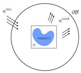
Figure 1: Scattering from a compact inhomogeneity (contrast function) $q(\mathbf{x})$: the support of $q(\mathbf{x})$ is assumed to lie within the domain $\Omega$ and impinged upon by an incoming field $u^{\emph{inc}}$, such as a plane wave. In the forward scattering problem, $q(\mathbf{x})$ is known and one seeks to compute the scattered field, either within $\Omega$ or in the far field - say, on the boundary $\partial\mathcal{B}$ of an enclosing disk $\mathcal{B}$. In the inverse scattering problem, $q(\mathbf{x})$ is unknown, and one seeks to determine it from measurements of the scattered field on $\partial\mathcal{B}$.

Definition 1.

Suppose that, for a fixed frequency $k$, a series of experiments is carried out, with $M$ distinct plane waves impinging on a domain $\Omega$ which contains the support of an unknown contrast function $q(\mathbf{x})$. Let the incident directions be denoted by $\{\mathbf{d}_{m},m=1,\dots,M\}$. The single frequency inverse scattering problem consists of determining $q(\mathbf{x})$ from $\{u^{{far}}_{k,\mathbf{d}_{m}}(\theta),m=1,\dots,M\}$.

It is important to note that, in the far field, no more than $O(k)$ independent measurements can reasonably be made on $\partial\mathcal{B}$, assuming the support of $q(\mathbf{x})$ has been normalized to have approximately unit diameter. This follows from either standard estimates for the behavior of the multipole expansion of $u^{\emph{scat}}_{k,\mathbf{d}_{m}}(\mathbf{x})$, or the Heisenberg uncertainty principle [24, 25, 26, 38]. In physical terms, the issue is that Fourier modes on $\partial\mathcal{B}$ whose frequency exceeds $k$ correspond to evanescent and rapidly decaying fields emanating from the scatterer. Acquiring such data would impose exponential accuracy requirements on the measurements of $u^{far}_{k,\mathbf{d}_{m}}(\theta)$. In short, only $O(k)$ linearly independent measurements are available for each angle of incidence with finite precision. Similar arguments show that only $O(k)$ independent directions of incidence are useful in probing the unknown inhomogeneity, leading to a total of $O(k^{2})$ independent measurements. Thus, in two dimensions, the single frequency inverse problem is at the limits of feasibility in seeking to reconstruct a model for $q(\mathbf{x})$ with $O(k^{2})$ unknowns.

Definition 2.

Suppose now that we probe the unknown function $q(\mathbf{x})$ at a set of frequencies $\{k_{j},\,j=1,\dots,Q\}$, with incident directions at each frequency $k_{j}$ denoted by $\{\mathbf{d}_{j,m},\,m=1,\dots,M_{j}\}$. The multi-frequency inverse scattering problem consists of determining $q(\mathbf{x})$ from $\{u^{far}_{k_{j},\mathbf{d}_{j,m}}(\theta);\,j=1,\dots,Q,\,m=1,\dots,M_{j}\}$.

Remark 1.2.

As indicated above, the number of linear independent measurements that can be made on ${\partial\mathcal{B}}$ is of the order $O(k_{j})$ at frequency $k_{j}$. We will denote by $P_{j}$ the number of distinct (equispaced) measurements made in the angular variable $\theta$. In practice, one could make a larger number of measurements and filter/denoise the data by fitting a Fourier series on ${\partial\mathcal{B}}$ with $P_{j}$ modes.

We assume $q(\mathbf{x})\in C_{0}(\Omega)$ and define the operator $\mathcal{F}_{k,\mathbf{d}}:C_{0}(\Omega)\rightarrow L^{2}(\partial\mathcal{B})$ by

$$\mathcal{F}_{k,\mathbf{d}}[q]=u^{\emph{far}}_{k,\mathbf{d}}.$$ (5)

The operator $\mathcal{F}$ is well-defined since the forward scattering problem is well-posed. To obtain the value of $u^{far}_{k,\mathbf{d}}$ at a point $\mathbf{x}=(R\cos\theta,R\sin\theta)$, one must solve (4) and (3) or its integral equation counterpart, the Lippmann-Schwinger equation [34, 63],

$$u_{q,k,\mathbf{d}}^{\text{\emph{scat}}}(\mathbf{x})+k^{2}\iint_{\Omega}G(\mathbf{x},\mathbf{y})q(\mathbf{y})(u_{q,k,\mathbf{d}}^{\text{\emph{scat}}}(\mathbf{y})+u^{\text{\emph{inc}}}(\mathbf{y},k,\mathbf{d}))\leavevmode\nobreak\ d{\mathbf{y}}=0,$$ (6)

with $G(\mathbf{x},\mathbf{y})=\frac{i}{4}H_{0}^{(1)}(k\|\mathbf{x}-\mathbf{y}\|)$ where $H_{0}^{(1)}(x)$ is the usual Hankel function of the first kind. Eq. (6) is derived by integrating both sides of (4) against $G(\mathbf{x},\mathbf{y})$, using the fact that it is the Green’s function for eq. (2) satisfying the radiation condition (3).

We will focus here on the multi-frequency inverse scattering problem defined above. In other words, our goal is to solve the nonlinear system of equations

$$\mathcal{F}_{k_{j},\mathbf{d}_{m}}[q]=u^{\emph{far}}_{k_{j},\mathbf{d}_{j,m}},$$ (7)

for $j=1,\dots,Q$, $m=1,\dots,M_{j}$. This is an ill-posed, nonlinear and nonconvex problem with a substantial literature (see, for example, [10, 34, 58] and the references therein). Broadly speaking, existing approaches can be classified as either iterative methods, derived from a nonlinear optimization framework, or direct methods, based on ideas drawn from image and signal processing. Iterative methods include variants of Newton’s method [24, 25, 26], the Gauss-Newton method [16, 17, 18], Landweber iteration [4, 5, 6, 8, 9, 11, 48], quasi-Newton methods [43, 44, 45], and the nonlinear conjugate gradient method [56, 57, 75]. Direct methods include decomposition methods [31, 35, 54, 65, 66, 68], the linear sampling method [20, 32], the singular source method [67, 68], the factorization method [51, 52], and the probe method of Ikehata [49]. Nevertheless, most numerical work on reconstruction has been limited to fairly simple contrast functions involving perhaps dozens of parameters in a model for the unknown contrast function $q(\mathbf{x})$.

In this paper, we are interested in developing a method for high-resolution two-dimensional applications, where $q(\mathbf{x})$ is modeled as a function on a grid with up to $100\times 100$ unknowns. We will make use of a Newton-like iterative method which relies on the frequency $k$ as a continuation parameter. More precisely, we will solve a sequence of single-frequency inverse problems for higher and higher values of $k$, using the approximation of $q(\mathbf{x})$ obtained at the preceding frequency as an initial guess. In the context of inverse scattering, such a scheme was first proposed by Chen [26] and is referred to as recursive linearization. More recent contributions include [5, 6, 8, 11]. The analogous problem for scattering from an unknown, impenetrable, sound-soft object is discussed in [13, 70, 71]. For time-domain versions of the problem, see [12, 73].

Remark 1.3.

The ill-posedness inherent in inverse scattering is closely tied to the issues stemming from the Heisenberg uncertainty principle discussed above. Loosely speaking, features of $q(\mathbf{x})$ that have frequency content greater than the probing incident field are evanescent and poorly determined by far field measurements. Overcoming this problem is often addressed by using some form of ad hoc regularization while solving the linearized subproblems which arise in the various reconstruction schemes [19, 34, 50, 53]. In the original work on recursive linearization [24, 25, 26], however, and in our previous work on inverse obstacle scattering [13], it was shown that the same stabilizing effect can be achieved by using a suitably band-limited model for the unknown. We will continue to employ that strategy here (see Section 3).

An outline of the paper follows. In Section 2, we describe the forward scattering problem and its solution using the fast direct solver developed in [41] - the so-called Hierarchical Poincaré-Steklov method. In Section 3, we describe our implementation of recursive linearization for the inverse problem and in Section 4, we illustrate the performance of our method. Section 5 contains some concluding remarks and a discussion of future directions for research.

2 The direct scattering problem

In this section, we briefly review the forward scattering problem and its solution for penetrable media in two dimensions. We assume that the index of refraction $1-q(\mathbf{x})$ is real and positive for $\mathbf{x}\in\Omega$, so that the problem has a unique solution for any $k>0$ [34].

We begin by observing that an alternative formulation for the original partial differential equation (1) is to consider an interior variable medium problem

$$\Delta u(\mathbf{x})+k^{2}(1-q(\mathbf{x}))u(\mathbf{x}) = 0\quad\mbox{in}\quad\Omega,$$

$$u(\mathbf{x}) = h(\mathbf{x})\quad\mbox{on}\quad\partial\Omega,$$ (8)

coupled with an exterior constant-coefficient problem

$$\Delta u^{scat}(\mathbf{x})+k^{2}u^{scat}(\mathbf{x}) = 0\quad\quad\mbox{in}\quad\mathbb{R}^{2}\setminus\Omega,$$ (9)

$$u^{scat}(\mathbf{x}) = s(\mathbf{x})\quad\quad\mbox{in}\quad\partial\Omega,$$

$$\frac{\partial u^{scat}}{\partial r}-iku^{scat} = o(r^{-1/2})\quad r=\|\mathbf{x}\|\rightarrow\infty.$$ (10)

For the sake of simplicity, let us assume that the interior Dirichlet problem does not have a resonance at the particular frequency $k$ under consideration. We then seek to find functions $h(\mathbf{x})$ and $s(\mathbf{x})$ so that gluing together the interior and exterior total fields yields a continuously differentiable total field $u(\mathbf{x})$. If that can be achieved, then the solution to (8) matches the solution to (1) in the interior of $\Omega$ and $u=u^{scat}+u^{inc}$ matches the solution to (1) in the exterior of $\Omega$ by a simple uniqueness argument [34].

To accomplish this matching, let $\frac{\partial u}{\partial n}$ denote the outward normal derivative of the solution to (8) on $\partial\Omega$. We may then define the interior “Dirichlet-to-Neumann” map $T^{int}$ by

$$T^{int}h=\frac{\partial u}{\partial n}.$$

There is also a well-defined exterior “Dirichlet-to-Neumann” map $T^{ext}$ such that

$$T^{ext}s=\frac{\partial u^{scat}}{\partial n}.$$

Given these two maps, it is straightforward to determine $s(\mathbf{x})$ and $h(\mathbf{x})$ by impose the continuity conditions

$$s(\mathbf{x})+u^{inc}(\mathbf{x}) =h$$

$$T^{ext}[s](\mathbf{x})+\frac{\partial u^{inc}}{\partial n}(\mathbf{x}) =T^{int}[h](\mathbf{x}).$$

In particular , we can obtain the scattered field $u^{scat}(\mathbf{x})=s(\mathbf{x})$ on $\partial\Omega$ by solving the problem (analogous to equation (2.12) in[55]):

$$\left(T^{int}-T^{ext}\right)u^{scat}|_{\partial\Omega}=\frac{\partial u^{inc}}{\partial n}-T^{int}u^{inc}|_{\partial\Omega}.$$

Remark 2.1.

While $T^{int}$ is rather complicated to describe, $T^{ext}$ can be written using standard layer potentials from Green’s formula, since the scattered field $u^{scat}(\mathbf{x})$ satisfies

$$u^{scat}(\mathbf{x})=Du^{scat}(\mathbf{x})-S\frac{\partial u^{scat}}{\partial n}(\mathbf{x})$$

for $\mathbf{x}$ in the exterior of $\Omega$. Here, $D\phi(\mathbf{x})=\int_{\partial\Omega}\frac{\partial G(\mathbf{x},\mathbf{y})}{\partial n_{y}}\phi(\mathbf{y})ds(\mathbf{y})$ and $S\phi(\mathbf{x})=\int_{\partial\Omega}G(\mathbf{x},\mathbf{y})\phi(\mathbf{y})ds(\mathbf{y})$ are the double and single layer operators, respectively and $G(\mathbf{x},\mathbf{y})=(i/4)H_{0}^{(1)}(k\|\mathbf{x}-\mathbf{y}\|)$. Using standard jump relations [33, 34], it is easy to verify that

$$T^{ext}=S^{-1}\left(D-\frac{I}{2}\right).$$

This is the essence of the approach used in the Hierarchical Poincaré-Steklov (HPS) solver of [41]. Without entering into details, we simply note here that the basic discretization, for $K$th order accuracy, involves superimposing a quad-tree on the domain $\Omega$, with tensor product $K\times K$ Chebyshev grids on each leaf node, used to represent both $u(\mathbf{x})$ and $q(\mathbf{x})$. The HPS method solves the interior problem on $\Omega$ by a recursive merging procedure, and represents the exterior field using a layer potential on $\partial\Omega$. By a careful use of “impedance-to-impedance” maps, the method involves well-conditioned operators and requires only $O(N^{3/2})$ work for factoring the system matrix with a given contrast function $q(\mathbf{x})$. Given that factorization, the solver requires only $O(N\log N)$ work in order to solve eq. (4) for each right-hand side defined by $u^{inc}$. (See the original paper [41] for a complete description of the method.)

Over the last decade, a number of fast direct solvers have been developed with the same basic complexity, some using direct discretization of the partial differential equation (PDE) and some using the Lippmann-Schwinger integral formulation. We will not attempt to review the literature here and refer the reader to [1, 2, 14, 15, 22, 27, 36, 37, 46, 47, 60, 77, 78] and the references therein.

The HPS solver was implemented in MATLAB and run in parallel mode using up to 12 cores of a system with 2.5GHz Intel Xeon CPUs. To illustrate its performance, Table 1 presents the run-time for a sequence of problems with increasing frequency $k$ and an increasing number of discretization points, using the simple contrast function

$$q(\mathbf{x})=q(x,y)=1.5\exp\left(-\frac{x^{2}+y^{2}}{50}\right)$$

in the domain $\Omega=[-\frac{\pi}{2},\frac{\pi}{2}]^{2}$. $N$ denotes the total number of points used to discretize the domain $\Omega$, and $N_{\partial\Omega}$ is the number of points used on the boundary $\partial\Omega$ for the solution of the exterior problem. $T_{\text{interior}}$, $T_{\text{bdry}}$ and $T_{\text{solve}}$ are the times (in seconds) to factor the interior system matrix, the exterior system matrix, and apply the resulting inverse, respectively.

$k$	$N$	$N_{\partial\Omega}$	$T_{\text{interior}}$	$T_{\text{bdry}}$	$T_{\text{solve}}$
1	3721	640	1.79e+00	1.94e+00	9.56e-04
2	3721	640	8.79e-01	1.70e+00	1.24e-03
4	3721	640	8.57e-01	1.71e+00	1.74e-03
8	14641	800	4.12e+00	2.24e+00	1.47e-03
16	58081	1120	1.66e+01	3.38e+00	2.95e-03
32	231361	1760	6.43e+01	5.96e+00	8.70e-03
64	923521	3040	2.66e+02	1.23e+01	2.16e-02
128	3690241	5600	1.10e+03	3.56e+01	8.71e-02

Table 1: Run times for the direct scattering problem with 16 points per wavelength.

Remark 2.2.

Note that the performance of the solver is independent of the wavenumber. Here the number of points per wavelength is kept fixed for consistency with experiments later where this choice guarantees a specific accuracy.

3 The inverse scattering problem

We turn now to the problem of recovering $q(\mathbf{x})$ from a set of far-field measurements of the scattered field. Instead of solving the full multi-frequency system of equations (7), we will proceed by solving a sequence of single frequency inverse problems. At each fixed frequency $k$, we assemble the scattered data for each of $M$ incident directions into the nonlinear system:

$${\bf F}_{k}[q]={\bf u}_{k}^{far},$$ (11)

where

$${\bf F}_{k}[q]\equiv\left[\begin{array}[]{c}\mathcal{F}_{k,\mathbf{d}_{1}}[q]\\ \mathcal{F}_{k,\mathbf{d}_{2}}[q]\\ \dots\\ \mathcal{F}_{k,\mathbf{d}_{M}}[q]\end{array}\right],\quad{\bf u}_{k}^{far}(\theta)\equiv\left[\begin{array}[]{c}u^{\emph{far}}_{k,\mathbf{d}_{1}}(\theta)\\ u^{\emph{far}}_{k,\mathbf{d}_{2}}(\theta)\\ \dots\\ u^{\emph{far}}_{k,\mathbf{d}_{M}}(\theta)\end{array}\right].$$ (12)

3.1 Linearization

Using Newton’s method, we linearize the problem (11) for $q(\mathbf{x})$ in the neighborhood of an initial guess $q_{0}(\mathbf{x})$. For this, let $\delta q=q-q_{0}$, so that we may write

$${\bf F}_{k}[q_{0}]+{\bf J}_{q_{0},k}\,\delta q\approx{\bf F}_{k}[q_{0}+\delta q]={\bf u}_{k}^{far},$$ (13)

leading to the linear system

$${\bf J}_{q_{0},k}\,\delta q={\bf u}_{k}^{far}-{\bf F}_{k}[q_{0}],$$ (14)

where ${\bf J}_{q_{0},k}$ is the Fréchet derivative of the operator ${\bf F}$ at $q_{0}$:

$${\bf J}_{q_{0},k}=\left[\begin{array}[]{c}J_{q_{0},k,\mathbf{d}_{1}}\\ J_{q_{0},k,\mathbf{d}_{2}}\\ \dots\\ J_{q_{0},k,\mathbf{d}_{M}}\end{array}\right].$$ (15)

Each block $J_{q_{0},k,\mathbf{d}_{m}}$ is the Fréchet derivative of the corresponding mapping $\mathcal{F}_{k,\mathbf{d}_{m}}[q_{0}]$, whose evaluation in terms of a scattering problem is described in Theorem 3. Eq. (14) is an overdetermined linear system of equations for the increment $\delta q$, assuming that $M\cdot P$ exceeds the number of degrees of freedom in the representation for $q(\mathbf{x})$, where $P$ denotes the number of equispaced measurements made in the angular variable on ${\partial\mathcal{B}}$. Since we will solve this system iteratively, we will need an algorithm for applying ${\bf J}_{q_{0},k}$ to a vector, as well as its adjoint ${\bf J}^{\ast}_{q_{0},k}$.

Theorem 3.

[34] Let $\mathbf{d}$ denote the angle of incidence of an incoming field $u^{inc}$ and let $u_{0}=u^{inc}+u_{0}^{scat}$ denote the solution to the scattering problem

$$\Delta u_{0}(\mathbf{x})+k^{2}(1-q_{0}(\mathbf{x}))u_{0}(\mathbf{x})=0$$ (16)

in $\mathbb{R}^{2}$, where $u_{0}^{scat}$ satisfies the Sommerfeld radiation condition. Let $\delta q$ be a given perturbation of $q_{0}$ and let $\mathcal{F}_{k,\mathbf{d}}[q_{0}]$ denote the far field operator (5). Then

$$J_{q_{0},k,\mathbf{d}}\,\delta q=v^{far}$$ (17)

where $v^{far}(\theta)=v(R\cos\theta,R\sin\theta)$ and $v(\mathbf{x})$ denotes the solution to the scattering problem

$$\Delta v(\mathbf{x})+k^{2}(1-q_{0}(\mathbf{x}))v(\mathbf{x})=k^{2}\,\delta q\,u_{0}$$ (18)

satisfying the Sommerfeld radiation condition.

Proof.

Let us write the solution to the scattering problem for the inhomogeneity $q_{0}+\delta q$ in the form

$$\Delta(u_{0}+v)+k^{2}(1-q_{0}-\delta q)(u_{0}+v)=0.$$

In that case, $v(\mathbf{x})$ is the change in the scattered field induced by the perturbation $\delta q$. The desired result follows after dropping quadratic terms. ∎

Theorem 4.

Let $f(\theta)$ denote a smooth function on the circle ${\partial\mathcal{B}}$ of radius $R$ and let $\chi(f,{{\partial\mathcal{B}}})$ denote the corresponding singular charge distribution on ${\partial\mathcal{B}}$ with charge density $f$, viewed as a generalized function in $\mathbb{R}^{2}$. Let $\mathbf{d}$ denote the direction of incidence of an incoming field $u^{inc}$, and let $q_{0}(\mathbf{x})$ denote a given inhomogeneity in $\Omega$. Then the adjoint operator $J^{\ast}_{q_{0},k,\mathbf{d}}:L^{2}(\partial\mathcal{B})\rightarrow C_{0}(\Omega)$ is given by

$$J^{\ast}_{q_{0},k,\mathbf{d}}\,f=\overline{u_{0}}\,w$$ (19)

where $u_{0}(\mathbf{x})$ denotes the solution to (16) and $w(\mathbf{x})$ is the solution to

$$\Delta w(\mathbf{x})+k^{2}(1-q_{0}(\mathbf{x}))w(\mathbf{x})=k^{2}\chi(f,{{\partial\mathcal{B}}})$$ (20)

in $\mathbb{R}^{2}$, satisfying the adjoint Sommerfeld radiation condition

$$\lim_{r\rightarrow\infty}\sqrt{r}\left(\frac{\partial w}{\partial r}+ikw\right)=0.$$

Proof.

We first integrate both sides of (18) against the conjugate of $w(\mathbf{x})$:

$$\iint_{\mathbb{R}^{2}}[\Delta v+k^{2}(1-q_{0})v]\overline{w}dA=\iint_{\Omega}k^{2}\,\delta q\,u_{0}\,\overline{w}dA.$$

Using Green’s second identity and the Sommerfeld radiation condition, it is straightforward to show that

$$\iint_{\mathbb{R}^{2}}[\Delta\overline{w}+k^{2}(1-q_{0})\overline{w}]vdA=\iint_{\Omega}k^{2}\,\delta q\,u_{0}\,\overline{w}dA.$$

or

$$\iint_{\mathbb{R}^{2}}\overline{\chi(f,{{\partial\mathcal{B}}})}\,v\,dA=\int_{\partial\mathcal{B}}\overline{f}\,v\,ds=\iint_{\Omega}\delta q\,u_{0}\,\overline{w}dA.$$

Since $\langle f,v,\rangle=\int_{\partial\mathcal{B}}\overline{f}\,v\,ds=\int_{\partial\mathcal{B}}\overline{f}\,J_{q_{0},k,\mathbf{d}}\delta q\,ds=\langle f,J_{q_{0},k,\mathbf{d}}\delta q\rangle$, it follows that

$$\langle J_{q_{0},k,\mathbf{d}}^{\ast}\,f,\delta q\rangle=\iint_{\Omega}\,\delta q\,u_{0}\,\overline{w}dA=\langle\overline{u_{0}}w,\delta q\rangle.$$

Since $\delta q$ is arbitrary, this yields the desired result. ∎

Definition 5.

We define the adjoint of ${\bf J}_{q,k}$ by

$${\bf J}^{\ast}_{q_{0},k}=\left[J^{\ast}_{q_{0},k,\mathbf{d}_{1}},J^{\ast}_{q_{0},k,\mathbf{d}_{2}},\dots,J^{\ast}_{q_{0},k,\mathbf{d}_{M}}\right].$$ (21)

3.2 Discretization and regularization at a fixed frequency

As noted in the introduction, at a given frequency $k$, we can only make $O(k^{2})$ independent measurements at finite precision, Thus, we seek to reconstruct a model for $q(\mathbf{x})$ with ${\rm supp}(q)\in[-\frac{\pi}{2},\frac{\pi}{2}]^{2}$ which has only $O(k^{2})$ free parameters.

This avoids various ad hoc regularization methods that are in common use. More precisely, at frequency $k$, we approximate the contrast function $q(x_{1},x_{2})$ restricted to the domain $\Omega=[-\frac{\pi}{2},\frac{\pi}{2}]^{2}$ by the function

$$q_{k}(x_{1},x_{2})=\sum_{\begin{subarray}{c}m_{1},m_{2}=1\\ m_{1}+m_{2}\leq S(k)\end{subarray}}^{S(k)}q_{m_{1},m_{2}}\sin\left(m_{1}\left(x_{1}+\frac{\pi}{2}\right)\right)\sin\left(m_{2}\left(x_{2}+\frac{\pi}{2}\right)\right),$$ (22)

with the maximum frequency $S(k)=\lfloor 2k\rfloor$. This representation has several useful features. Projection from a sampled function $q(\mathbf{x})$ onto the coefficients $\{q_{m_{1},m_{2}}\}$ can be accomplished in $O(N\log N)$ time using the nonuniform FFT (see [39, 42] and the references therein). $N$ here denotes the number of points in the discretization of $q(x_{1},x_{2})$. Moreover, the approximation is spectrally accurate for any smooth function $q(\mathbf{x})$ which has vanished together with all its derivatives at the boundary of $\Omega$.

Definition 6.

Let $\hat{q}(k)$ denote the vector of coefficients of the truncated sine series in (22). We denote by $\mathcal{E}_{k}$ the operator which evaluates the sine series given by the coefficients $\hat{q}(k)$ at points $\mathbf{x}\in\Omega$. We denote by $\mathcal{E}^{\ast}_{k}$ its adjoint.

3.3 Newton iteration

Suppose that we have an initial guess $q_{k}^{(0)}$ for the unknown contrast function, with far field measurements made at a fixed frequency $k$. Let $\widehat{\delta q}$ denote the vector of sine series coefficients which we will use to approximate the unknown perturbation $\delta q$. Newton’s method, for a tolerance $\epsilon$, proceeds as follows:

For $i=0,1,\dots$

1. Solve the linearized problem in a least squares sense using the normal equations:

   $${\mathcal{E}}_{k}^{\ast}{\bf J}_{q_{k}^{(i)},k}^{\ast}{\bf J}_{q_{k}^{(i)},k}\,{\mathcal{E}}_{k}\widehat{\delta q}={\mathcal{E}}_{k}^{\ast}{\bf J}_{q_{k}^{(i)},k}^{\ast}\left({\bf u^{\text{\emph{far}}}}-{\bf F}_{k}[q_{k}^{(i)}]\right).$$ (23)

2. Set $q_{k}^{(i+1)}=q_{k}^{(i)}+{\mathcal{E}}_{k}\widehat{\delta q}$.

3. Stop when $\|{\bf u^{\text{\emph{far}}}}-{\bf F}_{k}[q_{k}^{(i)}]\|<\epsilon$.

It is instructive, at this stage, to compute the work required at a single frequency $k$. At the $i$th Newton step, we must solve $M$ inhomogeneous Helmholtz equations to obtain the right-hand side for the system (23). Assuming that we solve the normal equations iteratively using, say, the conjugate gradient method, we must solve $2M$ inhomogeneous Helmholtz equations at each iteration to apply ${\bf J}_{q_{k}^{(i)},k}^{\ast}$ and ${\bf J}_{q_{k}^{(i)},k}$. Each of the PDEs, however, corresponds to a different right-hand-side in eqs. (18) or (20). Thus, using the HPS solver, we need only compute the factorization of the PDE once per Newton iteration. Thus, the total work is of the order $O(N_{newton}N^{3/2})+O(N_{newton}\,(2N_{iter}+1)\,M\,N)$, where $N$ denotes the number of grid points used in the solver.

3.4 Recursive Linearization

Our approach to the full multi-frequency inverse scattering problem (7) is now straightforward to describe. As noted above, it is based on Chen’s method of recursive linearization [5, 6, 8, 11, 24, 25, 26].

The essential insight of recursive linearization is the following; while (7) is a non-convex, nonlinear system of equations, if a band-limited approximation $q_{k}(\mathbf{x})$ of $q(\mathbf{x})$ were available and $\delta k$ is sufficiently small, then $q_{k}(\mathbf{x})$ is in the basin of attraction for Newton’s method in seeking the global minimum for $q_{k+\delta k}(\mathbf{x})$. We refer to the references cited above for a discussion of the theoretical foundations. Here, we describe an efficient implementation using all of the data corresponding to (7).

Recursive Linearization using Newton’s method We assume we have full aperture data for each of the frequencies $\{k_{1},k_{2},\dots,k_{Q}\}$ with $k_{1}<k_{2}<\dots<k_{Q}$. • Obtain an approximation $q_{k_{1}}$ for the contrast function $q(\mathbf{x})$ at the lowest available frequency using the Born approximation [6, 7, 21] or a direct imaging method like MUSIC or linear sampling [4]. • For $j=2,\ldots,Q$ – Create a uniform grid with $N=N(k_{j})$ points in the domain $\Omega$. – (Since the domain is $k_{j}/2$ wavelengths across, 10 points per wavelength requires a grid with $N\approx(5k_{j})^{2}$ points.) – Sample $q_{k_{j}}$ on the given grid. – Solve the single frequency system ${\bf F}_{k_{j}}[q]={\bf u}^{far}_{k_{j}}$ using Newton’s method
(section 3.3) with initial guess $q_{k_{j-1}}$. – Set $q_{k_{j}}$ to be the solution obtained by Newton’s method.

A crude estimate of the total work follows, assuming that $k_{Q}$ is the maximum frequency, that we take a step in frequency of $\delta k=O(1)$, that the number of Newton iterations $N_{newton}=1$ and that the number of iterations $N_{iter}$ required to solve the linear least squares problem is independent of frequency (see the next section). It is easy to see, under these hypotheses, that

$${\rm Work}\ \approx\ O(k_{Q}^{4})+(2N_{iter}+1)O(k_{Q}^{4})\,.$$

The first term is the work required to factor the linear system corresponding to the forward scattering problem for the initial guess $q_{k}$ at each successive frequency. The second term is the work required to solve all the scattering problems required in applying ${\bf J}_{q_{k},k}^{\ast}$ and ${\bf J}_{q_{k},k}$ at each iteration of the linearized problem.

4 Numerical experiments

In order to illustrate the performance of our method, we have chosen four examples of increasing complexity. In each case, we take a known function $q(\mathbf{x})$ and simulate the measured data on ${\partial\mathcal{B}}$ by solving the forward scattering problem. In order to avoid “inverse crimes”, we use a different solver for data generation than we do for inversion. In particular, instead of the HPS solver, we use the fast HODLR-based scheme [1] for the Lippmann-Schwinger integral equation with eight digits of accuracy.

We compute the data

$$u^{far}(\theta)=u^{scat}_{q,k_{j},\mathbf{d}_{j,m}}(R\cos\theta_{p},R\sin\theta_{p})$$

for $m=1,\dots,M_{j}$ at $R=20$ with $\theta_{p}=2\pi p/P_{j}$, for frequencies $k_{j}=1+j/4$, with $j=0,\ldots,Q$, where $M_{j}=\lfloor 2k_{j}\rfloor$, and $P_{j}=\lfloor 4k_{j}\rfloor$. The incident directions are chosen as $\mathbf{d}_{j,m}=\left(\cos\theta_{j,m},\sin\theta_{j,m}\right)$, where $\theta_{j,m}=2\pi m/M_{j}$.

In the first two examples, we use the scattered data computed from our forward solver. For the last two examples, noise in the form

$$\tilde{u}^{scat}_{q,k_{j},\mathbf{d}{j,m}}(\theta)=u^{scat}_{q,k_{j},\mathbf{d}{j,m}}(\theta)+\delta\dfrac{\|u^{scat}_{q,k_{j},\mathbf{d}{j,m}}(\theta)\|}{\|\epsilon_{1}+i\epsilon_{2}\|}(\epsilon_{1}+i\epsilon_{2})$$

is added, where $\epsilon_{1}$ and $\epsilon_{2}$ are normally distributed random variables with mean zero and variance one.

For each frequency $k_{j}$, we discretize the domain $\Omega$ with a uniform quad tree consisting of $2^{l}\times 2^{l}$ square leaf nodes with a $16\times 16$ grid used on each to represent $u(\mathbf{x})$ and $q(\mathbf{x})$. In examples 1 and 2, $l$ is chosen so that there are at least 10 points per wavelength in the discretization, yielding at least 5 digits of accuracy in the solver. In examples 3 and 4, $l$ is chosen so that there are at least 6 points per wavelength in the discretization, yielding at least 3 digits of accuracy.

For the sake of simplicity, rather than using the Born approximation or a direct imaging method [21, 4, 7, 6], we assume

$$q_{1}(x_{1},x_{2})=\sum_{\begin{subarray}{c}m_{1},m_{2}=1\\ m_{1}+m_{2}\leq 2\end{subarray}}^{2}q_{m_{1},m_{2}}\sin\left(m_{1}\left(x_{1}+\frac{\pi}{2}\right)\right)\sin\left(m_{2}\left(x_{2}+\frac{\pi}{2}\right)\right),$$

with $q_{1,1},q_{1,2},q_{2,1}$ given as the projection of $q(\mathbf{x})$ onto those modes.

For examples 1–4, we let $k_{Q}=14.25,9,70$, and $70$, respectively. Finally, we make use of the least squares solver LSQR [64] in MATLAB. It is algebraically identical to conjugate gradient on the normal equations and the performance of the two methods is very similar. All timings below are reported using our solver in conjunction with the parallel computing toolbox in MATLAB, which makes use of up to 32 cores of a 2.5GHz Intel Xeon system. Parallelization is straightforward, since the forward scattering problems are all uncoupled and dominate the CPU time.

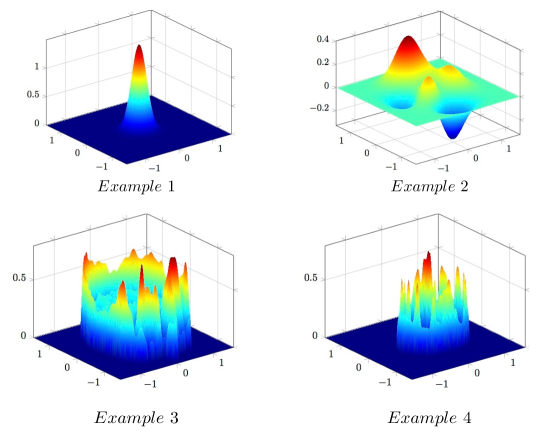
Figure 2: The contrast functions for our four examples.

Example 1: A single Gaussian.

First consider the case where the contrast function is a single Gaussian (Fig. 2):

$$q(x,y)=1.5\exp\left(-\frac{x^{2}+y^{2}}{50}\right).$$

The progress of recursive linearization is presented in Fig. 3, which shows contour plots of the exact solution next to the reconstructions at the lowest $k=1$, a mid-range $k=5$, and the highest $k=14.25$ frequencies. Below the contour plots are cross-sections of the reconstructed function along a single line: that is, $q(x,0)$ for $x\in\left[-\pi/2,\pi/2\right]$. Fig. 4 reports the $L^{2}$-error of the reconstruction and the condition number of the linearized least squares problem as the frequency increases. Note that the convergence is very rapid as a function of $k$, since the contrast is smooth and the component solvers are high order accurate. The total solution time required was about fifteen minutes.

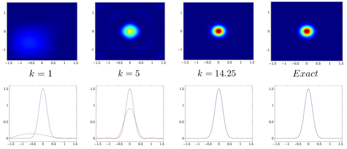
Figure 3: Recovering a simple Gaussian contrast function by recursive linearization (example 1). The upper row shows a contour plot of the estimated $q(\mathbf{x})$ at various frequencies as well as the exact contrast function. The lower row shows the corresponding plots of the reconstructed cross-section $q(x,0)$ for $x\in\left[-\pi/2,\pi/2\right]$. The reconstruction is shown in red and the original contrast is shown in blue.

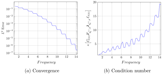
Figure 4: On the left, we plot the error $\|q_{k}-q\|$ in $L^{2}(\Omega)$ as a function of frequency. On the right, we plot the condition number of the linear least squares problem as a function of frequency.

Example 2: A sum of Hermite functions.

We next consider a contrast function made up of a sum of Hermite functions (Gaussians and their derivatives):

$$q(x,y) = 0.15\left(1-\frac{x}{\sigma}\right)^{2}\exp\left(-\left(\left(\frac{x}{\sigma}\right)^{2}+\left(\frac{y}{\sigma}+1\right)^{2}\right)\right)-\frac{1}{60}\exp\left(-\left(\left(\frac{y}{\sigma}\right)^{2}+\left(\frac{x}{\sigma}+1\right)^{2}\right)\right)$$

$$-\sigma\left(0.4x-\left(\frac{x}{\sigma}\right)^{3}-\left(\frac{y}{\sigma}\right)^{5}\right)\exp\left(-\left(\frac{x^{2}+y^{2}}{\sigma^{2}}\right)\right).$$

where $\sigma=0.5$ (Fig. 2). While the contrast function in this example is, in some sense, more complicated than a simple Gaussian, it is a smoother function. Thus, high fidelity is already achieved at $k=9$. The progress of recursive linearization is presented in Fig. 5, which shows contour plots of the reconstruction at frequencies $k=1,5,$ and $9$, as well as the exact solution. The figure also reports the $L^{2}$-error of the reconstruction and the condition number of the linearized least squares problem verses frequency. Again, the convergence is very rapid as a function of $k$, since the contrast is smooth and the component solvers are high order accurate. The total solution time required was about ten minutes.

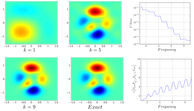
Figure 5: Recovering a sum of Gaussians by recursive linearization (example 2). Contour plots of the estimated $q(\mathbf{x})$ are shown at frequencies $k=1$, $k=5$, and $k=9$, as well as the exact solution. On the right, we also plot the error $\|q_{k}-q\|$ in $L^{2}(\Omega)$ and the the condition number of the linear least squares problem as functions of frequency.

Example 3: Axial cross-section of head.

For a more interesting (and higher frequency) model, we constructed a contrast function that resembles the axial cross section of a human head at the level of the orbitals (a simulated head phantom). A surface plot of the contrast function is shown in Fig. 2 (labeled example 3) and a contour plot in Fig. 6 (labeled Exact). Fig. 6 also illustrates the progress of recursive linearization at frequencies $k=1,10,25,50,$ and $70$. As mentioned previously, our simulated data was computed with 6 points per wavelength in the discretization, and 5% noise was added before reconstruction.

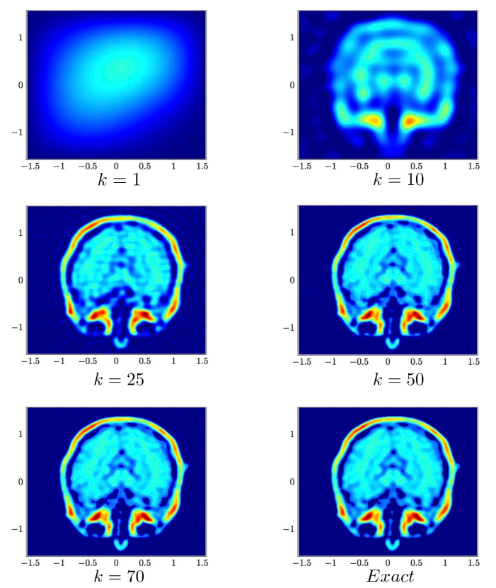
Figure 6: Recovering a simulated head phantom by recursive linearization (example 3). The estimated contrast function $q(\mathbf{x})$ is shown at frequencies $k=1$, $k=10$, $k=25$, $k=50$, and $k=70$.

Fig. 7 reports (a) the $L^{2}$-error of the reconstruction, (b) the condition number of the linearized system, (c) the number of the LSQR iterations required and (d) the time in seconds it takes the procedure to create the approximate contrast function versus the frequency. The $L^{2}$-error, the number of LSQR iterations and the solution time results are reported for the problem with and without $\delta=0.05$ noise.

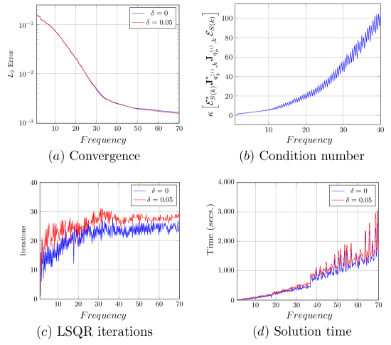
Figure 7: Numerical results for the simulated axial cross section of a head (example 3). In (a), we plot the $L^{2}$ error $\|q_{k}-q\|$ as a function of frequency. In (b), we plot the condition number of the linearized least squares problem and in (c) we show the number of LSQR iterations required. In (d), we plot the CPU time required at each frequency during the reconstruction process.

Table 2 provides a more detailed breakdown of the run time for the recursive procedure (using simulated data with 5% noise). Here, $N$ represents the total number of points used to discretize the domain $\Omega$, $Modes=S(k)*[S(k)+1]/2$ is the number of modes used as unknowns in the linear least squares problem, $M$ is the number of incidence directions used, $M\cdot P$ is the number of incident directions times the number of receiver locations for each $k$, $T_{f}$ is the time (in secs.) spent factoring the discretized forward problem for a given contrast function $q_{k}$, $N_{it}$ is the number of iterations necessary for the LSQR method to converge with a tolerance of $\epsilon=10^{-3}$, and $T_{l}$ is the time (in secs.) to solve eq. (23) at the indicated frequency, and $T_{t}$ is the cumulative time needed for the full recursion up to the indicated value of $k$, with steps of $\delta k=0.25$.

$k$	$N$	$Modes$	$M$	$M\cdot P$	$T_{f}$	$N_{it}$	$T_{l}$	$T_{t}$
1.00	3721	1	2	16	7.77	11	6.81	12.34
2.00	3721	6	4	64	2.95	20	20.82	59.97
4.00	3721	28	8	256	2.93	23	44.58	233.36
8.00	3721	120	16	1024	2.90	25	92.41	918.20
16.00	3721	496	32	4096	2.99	27	195.14	4109.56
32.00	14641	2016	64	16384	6.44	30	515.72	22603.09
64.00	58081	8128	128	65536	25.97	28	1412.77	151114.44

Table 2: Performance of recursive linearization for the simulated head phantom.

Example 4: Axial cross-section of thorax.

For our last example, we constructed a contrast function that simulates the axial cross section of a human thorax at the level of the heart. A surface plot of the contrast function is shown in Fig. 2 (labeled Example 4) and a contour plot in Fig. 8 (labeled Exact). Fig. 8 also shows the progress of recursive linearization at frequencies $k=1,10,25,50,$ and $70$. The simulated data was computed with 6 points per wavelength in the discretization, and we added 5% noise before reconstruction.

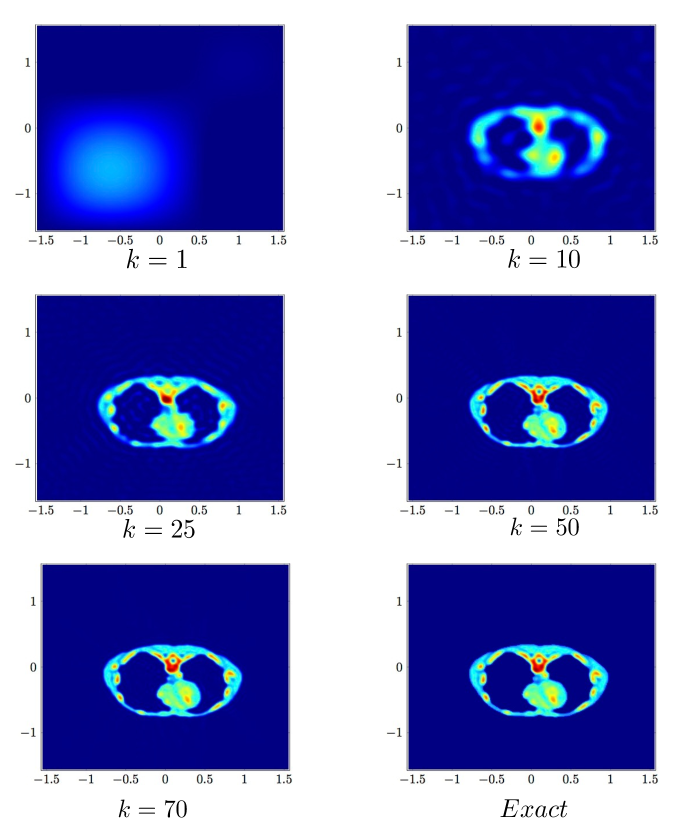
Figure 8: Recovering a simulated thorax phantom by recursive linearization (example 4). The estimated contrast function $q(\mathbf{x})$ is shown at frequencies $k=1$, $k=10$, $k=25$, $k=50$, and $k=70$.

Fig. 9 reports (a) the $L^{2}$-error of the reconstruction, (b) the condition number of the linearized system, (c) the number of the LSQR iterations required and (d) the time in seconds it takes the procedure to create the approximate contrast function versus the frequency. The $L^{2}$-error, the number of LSQR iterations and the solution time results are reported for the problem with and without $\delta=0.05$ noise.

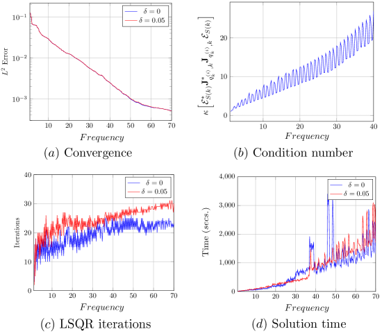
Figure 9: Numerical results for the simulated axial cross section of a thorax (example 4). In (a), we plot the $L^{2}$ error $\|q_{k}-q\|$ as a function of frequency. In (b), we plot the condition number of the linearized least squares problem and in (c) we show the number of LSQR iterations required. In (d), we plot the CPU time required at each frequency during the reconstruction process.

Table 3 reports a more detailed breakdown of the run time for the recursive procedure (using simulated data with 5% noise). The same notation is used as in Example 3.

$k$	$N$	$Modes$	$M$	$M\cdot P$	$T_{f}$	$N_{it}$	$T_{l}$	$T_{t}$
1.00	3721	1	2	16	7.57	8	5.56	22.73
2.00	3721	6	4	64	2.73	17	17.47	78.08
4.00	3721	28	8	256	3.12	19	37.19	258.55
8.00	3721	120	16	1024	2.95	21	77.81	995.52
16.00	3721	496	32	4096	3.07	26	188.05	3638.91
32.00	14641	2016	64	16384	6.48	23	391.33	24038.52
64.00	58081	8128	128	65536	25.07	29	1469.23	172365.71

Table 3: Performance of recursive linearization for the simulated thorax phantom.

5 Conclusions

We have presented a fast, stable algorithm for inverse scattering: reconstructing an unknown sound speed from far field measurements of the scattered field, in a fully nonlinear regime. For this, we have combined Chen’s method of recursive linearization with a recently developed, spectrally accurate fast direct solver [41]. A remarkable feature of recursive linearization is that by solving a sequence of linearized problems for sufficiently small steps in frequency (for a commensurate, band-limited model), one avoids the difficulties associated with the fact that the high-frequency problem is non-convex and ill-posed. Using the HPS solver of [41], the CPU time requirements for our scheme are modest and we believe that the reconstructions shown here are among the largest ever computed. It is worth noting that for the two large-scale problems considered above, approximately one million partial differential equations were solved, requiring approximately two days in our current parallel MATLAB implementation (using up to 30 cores).

In our experiments, Newton’s method requires several iterations at the lowest frequency, when the initial guess is far from the desired minimum. As the frequency increases, however, a single Newton iteration is sufficient, consist with the underlying theory [11, 17, 26].

Recursive linearization is easily extended to acoustic or electromagnetic scattering three dimensions. All aspects of the scheme described above have clear three-dimensional analogs. Fast, direct solvers, however, are still under active development and the scale of the problem is substantially larger, of course, for a fixed resolution in each linear dimension.

The scheme described here can be improved and accelerated in various ways and serves mainly as a “proof of concept”. Two important issues we have not addressed concern limitations on the available data; in many settings, only partial aperture data is available and in many regimes, only the magnitude of the scattered field can be measured, not its phase. We are currently working on extensions of the method to such problems.

References

- [1] S. Ambikasaran, C. Borges, L. Imbert-Gerard, and L. Greengard, Fast, adaptive, high order accurate discretization of the lippmann-schwinger equation in two dimension, eprint arXiv:1505.07157, (2015).
- [2] S. Ambikasaran and E. Darve, An Fast Direct Solver for Partial Hierarchically Semi-Separable Matrices, Journal of Scientific Computing, (2013), pp. 1–25.
- [3] R.C. Aster, B. Borchers, and C.H. Thurber, Parameter Estimation and Inverse Problems, Academic Press, Academic Press, 2013.
- [4] G. Bao, S. Hou, and P. Li, Inverse scattering by a continuation method with initial guesses from a direct imaging algorithm, Journal of Computational Physics, 227 (2007), pp. 755–762.
- [5] G. Bao and P. Li, Inverse medium scattering for the Helmholtz equation at fixed frequency, Inverse Problems, 21 (2005), pp. 1621–1641.
- [6] , Inverse Medium Scattering Problems for Electromagnetic Waves, SIAM Journal on Applied Mathematics, 65 (2005), pp. 2049–2066.
- [7] , Inverse medium scattering problems in near-field optics, Journal of Computational Mathematics, 25 (2007), pp. 252–265.
- [8] , Numerical solution of an inverse medium scattering problem for Maxwell’s Equations at fixed frequency, Journal of Computational Physics, 228 (2009), pp. 4638–4648.
- [9] , Shape Reconstruction of Inverse Medium Scattering for the Helmholtz Equation, in Computational Methods for Applied Inverse Problems, Y. Bai, G. Bao, and J. J. Cao et al., eds., De Gruyter, Berlin, Boston, 2012, pp. 283–306.
- [10] G. Bao, P. Li, J. Lin, and F. Triki, Inverse scattering problems with multi-frequencies, Inverse Problems, 31 (2015), p. 093001.
- [11] G. Bao and F. Triki, Error Estimates for the Recursive Linearization of Inverse Medium Problems, Journal of Computational Mathematics, 28 (2010), pp. 725–744.
- [12] L. Beilina, N. T. Thanh, M. V. Klibanov, and J. B. Malmberg, Globally convergent and adaptive finite element methods in imaging of buried objects from experimental backscattering radar measurements, Journal of Computational and Applied Mathematics, 289 (2015), pp. 371 – 391. Sixth International Conference on Advanced Computational Methods in Engineering (ACOMEN 2014).
- [13] C. Borges and L. Greengard, Inverse obstacle scattering in two dimensions with multiple frequency data and multiple angles of incidence, SIAM J. Imaging Sciences, 8 (2015), pp. 280–298.
- [14] S. Börm, L. Grasedyck, and W. Hackbusch, Hierarchical matrices, Lecture notes, 21 (2003).
- [15] , Introduction to hierarchical matrices with applications, Engineering Analysis with Boundary Elements, 27 (2003), pp. 405–422.
- [16] T. Bui-Thanh and O. Ghattas, Analysis of the hessian for inverse scattering problems, part i: Inverse shape scattering of acoustic waves, 2013 Highlight Collection of Inverse Problems, 28 (2012), p. 055001.
- [17] , Analysis of the hessian for inverse scattering problems, part ii: Inverse medium scattering of acoustic waves, Inverse Problems, 28 (2012), p. 055002.
- [18] , Analysis of the hessian for inverse scattering problems part iii: Inverse medium scattering of electromagnetic waves in three dimensions, Inverse Problems and Imaging, 7 (2013), p. 1139–1155.
- [19] F. Cakoni and D. Colton, Qualitative Methods in Inverse Scattering Theory: An Introduction, Interaction of Mechanics and Mathematics, Springer, 2006.
- [20] F. Cakoni, D. Colton, and P. Monk, The Linear Sampling Method in Inverse Electromagnetic Scattering, Society for Industrial and Applied Mathematics, 2011.
- [21] S. Chaillat and G. Biros, FaIMS: A fast algorithm for the inverse medium problem with multiple frequencies and multiple sources for the scalar Helmholtz equation, Journal of Computational Physics, 231 (2012), pp. 4403–4421.
- [22] S. Chandrasekaran, P. Dewilde, M. Gu, W. Lyons, and T. Pals, A fast solver for HSS representations via sparse matrices, SIAM Journal on Matrix Analysis and Applications, 29 (2006), pp. 67–81.
- [23] G. Chavent, G. Papanicolaou, P. Sacks, and W. Symes, Inverse Problems in Wave Propagation, The IMA Volumes in Mathematics and its Applications, Springer New York, 2012.
- [24] Y. Chen, Recursive linearization for inverse scattering, Tech. Report Yale Research Report/DCS/RR-1088, Department of Computer Science, Yale University, New Haven, CT, October 1995.
- [25] , Inverse scattering via heisenberg’s uncertainty principle, Tech. Report Yale Research Report/DCS/RR-1091, Department of Computer Science, Yale University, New Haven, CT, February 1996.
- [26] , Inverse scattering via Heisenberg’s uncertainty principle, Inverse Problems, 13 (1997), pp. 253–282.
- [27] , A fast, direct algorithm for the Lippmann–Schwinger integral equation in two dimensions, Advances in Computational Mathematics, 16 (2002), pp. 175–190.
- [28] M. Cheney and B. Borden, Fundamentals of Radar Imaging, CBMS-NSF Regional Conference Series in Applied Mathematics, Society for Industrial and Applied Mathematics, 2009.
- [29] M. D. Collins and W. A. Kuperman, Inverse problems in ocean acoustics, Inverse Problems, 10 (1994), p. 1023.
- [30] R. Collins, Nondestructive Testing of Materials, Studies in applied electromagnetics and mechanics, IOS Press, 1995.
- [31] D. Colton and A. Kirsch, An approximation problem in inverse scattering theory, Applicable Analysis, 41 (1991), pp. 23–32.
- [32] , A simple method for solving inverse scattering problems in the resonance region, Inverse Problems, 12 (1996), pp. 383–393.
- [33] D. Colton and R. Kress, Integral equation methods in scattering theory, Pure and applied mathematics, Wiley, 1983.
- [34] , Inverse Acoustic and Electromagnetic Scattering Theory, Springer, 2 ed., 1998.
- [35] D. Colton and P. Monk, The inverse scattering problem for time-harmonic acoustic waves in an inhomogeneous medium, The Quarterly Journal of Mechanics and Applied Mathematics, 41 (1988), pp. 97–125.
- [36] E. Corona, P.-G. Martinsson, and D. Zorin, An direct solver for integral equations on the plane, Applied and Computational Harmonic Analysis, 38 (2015), pp. 284–317.
- [37] P. Coulier, H. Pouransari, and E. Darve, The inverse fast multipole method: using a fast approximate direct solver as a preconditioner for dense linear systems, ArXiv e-prints, (2015).
- [38] W. Crutchfield, Z. Gimbutas, L. Greengard, J. Huang, V. Rokhlin, N. Yarvin, and J. Zhao, Remarks on the implementation of wideband fmm for the helmholtz equation in two dimensions, Contemporary Mathematics, 408 (2006), pp. 99–110.
- [39] A. Dutt and V. Rokhlin, Fast Fourier transforms for nonequispaced data, SIAM Journal on Scientific Computing, 14 (1993), pp. 1368–1393.
- [40] H. Engl, A.K. Louis, and W. Rundell, Inverse Problems in Medical Imaging and Nondestructive Testing: Proceedings of the Conference in Oberwolfach, Federal Republic of Germany, February 4–10, 1996, Springer Vienna, 2012.
- [41] A. Gillman, A. Barnett, and P. Martinsson, A spectrally accurate direct solution technique for frequency-domain scattering problems with variable media, BIT Numerical Mathematics, 55 (2014), pp. 141–170.
- [42] L. Greengard and J.-Y. Lee, Accelerating the nonuniform fast Fourier transform, SIAM Review, 46 (2004), pp. 443–454.
- [43] S. Gutman and M. Klibanov, Regularized quasi-newton method for inverse scattering problems, Mathematical and Computer Modelling, 18 (1993), pp. 5 – 31.
- [44] , Two versions of quasi-newton method for multidimensional inverse scattering problem, Journal of Computational Acoustics, 01 (1993), pp. 197–228.
- [45] , Iterative method for multi-dimensional inverse scattering problems at fixed frequencies, Inverse Problems, 10 (1994), p. 573.
- [46] W. Hackbusch, L. Grasedyck, and S. Börm, An introduction to hierarchical matrices, Max-Planck-Inst. für Mathematik in den Naturwiss., 2001.
- [47] K. L. Ho and L. Greengard, A fast direct solver for structured linear systems by recursive skeletonization, SIAM Journal on Scientific Computing, 34 (2012), pp. 2507–2532.
- [48] T. Hohage, On the numerical solution of a three-dimensional inverse medium scattering problem, Inverse Problems, 17 (2001), pp. 1743–1763.
- [49] M. Ikehata, Reconstruction of an obstacle from the scattering amplitude at a fixed frequency, Inverse Problems, 14 (1998), pp. 949–954.
- [50] J. Kaipio and E. Somersalo, Statistical and Computational Inverse Problems, Applied Mathematical Sciences, Springer, 2010.
- [51] A. Kirsch, An Introduction to the Mathematical Theory of Inverse Problems, Applied Mathematical Sciences, Springer New York, 1996.
- [52] , Characterization of the shape of a scattering obstacle using the spectral data of the far field operator, Inverse Problems, 14 (1998), pp. 1489–1512.
- [53] , An Introduction to the Mathematical Theory of Inverse Problems, Applied Mathematical Sciences, Springer, 2011.
- [54] A. Kirsch and R. Kress, An optimization method in inverse acoustic scattering, Boundary Elements IX, 3 (1987), pp. 3–18.
- [55] A. Kirsch and P. Monk, An analysis of the coupling of finite-element and Nyström methods in acoustic scattering, IMA J. Numer. Anal., 14 (1994), pp. 523–544.
- [56] R. E. Kleinman and P. M. van den Berg, A modified gradient method for two- dimensional problems in tomography, Journal of Computational and Applied Mathematics, 42 (1992), pp. 17 – 35.
- [57] , An extended range-modified gradient technique for profile inversion, Radio Science, 28 (1993), pp. 877–884.
- [58] R. Kress, Uniqueness and numerical methods in inverse obstacle scattering, Journal of Physics: Conference Series, 73 (2007), p. 012003.
- [59] P. Kuchment, The Radon Transform and Medical Imaging, CBMS-NSF Regional Conference Series in Applied Mathematics, Society for Industrial and Applied Mathematics, 2014.
- [60] P.-G. Martinsson, A direct solver for variable coefficient elliptic pdes discretized via a composite spectral collocation method, Journal of Computational Physics, 242 (2013), pp. 460–479.
- [61] J. Modersitzki and S. Wirtz, Registration of histological serial sectionings, in Mathematical Models for Registration and Applications to Medical Imaging. Mathematics in Industry, Otmar Scherzer, ed., New York, 2006, Springer.
- [62] M.Z. Nashed and O. Scherzer, Inverse Problems, Image Analysis, and Medical Imaging: AMS Special Session on Interaction of Inverse Problems and Image Analysis, January 10-13, 2001, New Orleans, Louisiana, Contemporary mathematics - American Mathematical Society, American Mathematical Society, 2002.
- [63] J.-C. Nédélec, Acoustic and Electromagnetic Equations, Springer, 2001.
- [64] C. C. Paige and M. A. Saunders, Lsqr: An algorithm for sparse linear equations and sparse least squares, ACM Transactions on Mathematical Software (TOMS), 8 (1982), pp. 43–71.
- [65] R. Potthast, A fast new method to solve inverse scattering problems, Inverse Problems, 12 (1996), pp. 731–742.
- [66] , A point source method for inverse acoustic and electromagnetic obstacle scattering problems, IMA Journal of Applied Mathematics, 61 (1998), pp. 119–140.
- [67] , Stability estimates and reconstructions in inverse acoustic scattering using singular sources, Journal of Computational and Applied Mathematics, 114 (2000), pp. 247–274.
- [68] , Point Sources and Multipoles in Inverse Scattering Theory, Chapman & Hall/CRC Research Notes in Mathematics, Taylor & Francis Group, 2001.
- [69] O. Scherzer, Handbook of Mathematical Methods in Imaging, Handbook of Mathematical Methods in Imaging, Springer New York, 2010.
- [70] M. Sini and N. T. Thanh, Convergence rates of recursive newton-type methods for multifrequency scattering problems, arXiv preprint arXiv:1310.5156, (2013).
- [71] , Inverse acoustic obstacle scattering problems using multifrequency measurements, Inverse Problems and Imaging, 6 (December 2012), pp. 749–773.
- [72] A. Tarantola, Inverse Problem Theory: Methods for Data Fitting and Model Parameter Estimation, Elsevier Science, 2013.
- [73] N. T. Thanh, L. Beilina, M. V. Klibanov, and M. A. Fiddy, Imaging of buried objects from experimental backscattering time-dependent measurements using a globally convergent inverse algorithm, SIAM Journal on Imaging Sciences, 8 (2015), pp. 757–786.
- [74] E. Ustinov, Encyclopedia of Remote Sensing, Springer New York, New York, NY, 2014, ch. Geophysical Retrieval, Inverse Problems in Remote Sensing, pp. 247–251.
- [75] P. M. van den Berg and R. E. Kleinman, A contrast source inversion method, Inverse Problems, 13 (1997), p. 1607.
- [76] Y. Wang, Regularization for inverse models in remote sensing, Progress in Physical Geography, 36 (2012), pp. 38–59.
- [77] J. Xia, S. Chandrasekaran, M. Gu, and X.S. Li, Fast algorithms for hierarchically semiseparable matrices, Numerical Linear Algebra with Applications, 17 (2010), pp. 953–976.
- [78] L. Zepeda-Núñez and H. Zhao, Fast alternating bi-directional preconditioner for the 2d high-frequency lippmann-schwinger equation, arXiv preprint arXiv:1602.07652, (2016).