Abstract

The main step in numerical evaluation of classical $\operatorname{Sl}_{2}(\mathbb{Z})$ modular forms is to compute the sum of the first $N$ nonzero terms in the sparse $q$-series belonging to the Dedekind eta function or the Jacobi theta constants. We construct short addition sequences to perform this task using $N+o(N)$ multiplications. Our constructions rely on the representability of specific quadratic progressions of integers as sums of smaller numbers of the same kind. For example, we show that every generalized pentagonal number $c\geq 5$ can be written as $c=2a+b$ where $a,b$ are smaller generalized pentagonal numbers. We also give a baby-step giant-step algorithm that uses $O(N/\log^{r}N)$ multiplications for any $r>0$, beating the lower bound of $N$ multiplications required when computing the terms explicitly. These results lead to speed-ups in practice.

1 Motivation and main results

We consider the problem of numerically evaluating a function given by a power series $f(q)=\sum_{n=0}^{\infty}c_{n}q^{e_{n}}$, where the exponent sequence $E=\{e_{n}\}_{n=0}^{\infty}$ is a strictly increasing sequence of natural numbers. If $|c_{n}|\leq c$ for all $n$ and the given argument $q$ satisfies $|q|\leq 1-\delta$ for some fixed $\delta>0$, then the truncated series taken over the exponents $e_{n}\leq T$ gives an approximation of $f(q)$ with error at most $c|q|^{T+1}/\delta$, which is accurate to $\Omega(T)$ digits. This brings us to the question of how to evaluate the finite sum $f(q)\approx\sum_{e_{n}\leq T}c_{n}q^{e_{n}}$ as efficiently as possible. To a first approximation, it is reasonable to attempt to minimize the total number of multiplications, including coefficient multiplications and multiplications by $q$.

Our work is motivated by the case $c_{n}$, $q\in\mathbb{C}$, but most statements transfer to rings such as $\mathbb{Q}_{p}$ and $\mathbb{C}[[t]]$. The abstract question of how to evaluate truncated power series, that is, polynomials, with a minimum number of multiplications may even be asked for an arbitrary coefficient ring. We review a number of generic approaches in §2.

More precisely, we are interested in highly structured exponent sequences, namely, sequences given by values of specific quadratic polynomials that belong to the Jacobi theta constants and to the Dedekind eta function. Exploiting this structure, one may hope to obtain more efficient algorithms.

The general one-dimensional theta function is given by

$$\vartheta(\tau,z)=\sum_{n\in\mathbb{Z}}e^{\pi in^{2}\tau+2\pi inz}=\sum_{n\in\mathbb{Z}}w^{n}q^{n^{2}}$$ (1)

with $q=e^{\pi i\tau}$ and $w=e^{2\pi iz}$ for $z\in\mathbb{C}$ and $\tau$ in the upper complex half-plane, that is, $\Im(\tau)>0$. For some $\ell\in\mathbb{Z}_{\geq 1}$ and $a$, $b\in\frac{1}{\ell}\mathbb{Z}$, the theta function of level $\ell$ and with characteristic $(a,b)$ is defined as

$$\vartheta_{a,b}(\tau,z)=e^{\pi ia^{2}\tau+2\pi a(z+b)}\vartheta(\tau,z+a\tau+b)=\sum_{n\in\mathbb{Z}}e^{\pi i(n+a)^{2}\tau+2\pi i(n+a)(z+b)}.$$

The functions of level $2$ are the classical Jacobi theta functions. Of special interest are the theta constants, the functions of $\tau$ in which one has fixed $z=0$ or $w=1$, respectively, and in particular, those of level $2$, given by

$$\vartheta_{0}(\tau) =\vartheta_{0,0}(\tau,0)=\sum_{n\in\mathbb{Z}}q^{n^{2}}=1+2\sum_{n=1}^{\infty}q^{n^{2}}=1+2q\sum_{n=1}^{\infty}q^{n^{2}-1},$$

$$\vartheta_{1}(\tau) =\vartheta_{0,\frac{1}{2}}(\tau,0)=1+2\sum_{n=1}^{\infty}(-1)^{n}q^{n^{2}},$$ (2)

$$\vartheta_{2}(\tau) =\vartheta_{\frac{1}{2},0}(\tau,0)=2\sum_{n=1}^{\infty}q^{\frac{1}{4}(2n+1)^{2}}=2q^{\frac{1}{4}}\sum_{n=1}^{\infty}q^{n(n+1)}.$$

(Here and in the following, when $q$ is defined as $q=e^{\gamma}$, by a slight abuse of notation we write $q^{\frac{1}{\ell}}$ for the then unambiguously defined $e^{\gamma/\ell}$.) The remaining function $\vartheta_{\frac{1}{2},\frac{1}{2}}(\tau,0)$ is identically $0$.

Different notational conventions are often used in the literature; the functions we have denoted by $\vartheta_{0},\vartheta_{1},\vartheta_{2}$ are sometimes denoted $\vartheta_{3},\vartheta_{4},\vartheta_{2}$ and often with different factors $\tfrac{1}{2}$ or $\pi$ among the arguments. Higher-dimensional theta functions are the objects of choice for studying higher-dimensional abelian varieties [31, 32, 33].

In dimension $1$, that is, in the context of elliptic curves, the Dedekind eta function is often more convenient [39, 37, 16, 17, 15]. It is a modular form of weight $\frac{1}{2}$ and level $24$ defined by

$$\eta(\tau) =q^{\frac{1}{24}}\prod_{n=1}^{\infty}(1-q^{n})=q^{\frac{1}{24}}\sum_{n=-\infty}^{\infty}(-1)^{n}q^{n(3n-1)/2}\quad\cite[cite]{[\@@bibref{}{Euler83}{}{}]}$$

$$=q^{\frac{1}{24}}\left(\sum_{n=1}^{\infty}(-1)^{n}q^{n(3n-1)/2}+\sum_{n=0}^{\infty}(-1)^{n}q^{n(3n+1)/2}\right)$$ (3)

for $q=e^{2\pi i\tau}$ (where an additional $2$ appears in the exponent compared to the definition of $q$ for theta functions). It is related to theta functions via $2\eta(\tau)^{3}=\vartheta_{0}(\tau)\vartheta_{1}(\tau)\vartheta_{2}(\tau)$ [39, §34, (10) and (11)], and $\eta(\tau)=\zeta_{12}\,\vartheta_{-\frac{1}{6},\frac{1}{2}}(3\tau,0)$ with $\zeta_{12}=e^{2\pi i/12}$. The latter property can be proved easily as an equality of formal series.

Other functions that can be expressed in terms of theta functions include Eisenstein series $G_{2k}(\tau)$ and the Weierstrass elliptic function $\wp(z;\tau)$. Theta functions are also useful in physics for solving the heat equation.

Another motivation for looking at theta and eta functions comes from complex multiplication of elliptic curves. The moduli space of complex elliptic curves is parameterized by the j-invariant, given by a $q$-series $j(\tau)=\frac{1}{q}+744+196884q+21493760q^{2}+\cdots$ for $q=e^{2\pi i\tau}$, which can be obtained explicitly from the series of the theta or eta functions as [39, §54, (5); §34, (11)]

$$j=\left(\frac{f_{1}^{24}+16}{f_{1}^{8}}\right)^{3}\text{ with }f_{1}(\tau)=\frac{\eta(\tau/2)}{\eta(\tau)},$$

or [39, §34, (10) and (11); §54, (6); §21, (14)]

$$j=32\,\frac{(\vartheta_{0}^{8}+\vartheta_{1}^{8}+\vartheta_{2}^{8})^{3}}{(\vartheta_{0}\vartheta_{1}\vartheta_{2})^{8}}.$$ (4)

The series for $j$ is dense, and the coefficients in front of $q^{n}$ asymptotically grow as $2^{1/2}n^{-3/4}e^{4\pi\sqrt{n}}$ [35]; so it is in fact preferable to obtain its values from values of theta and eta functions: Their sparse series imply that $O(\sqrt{T})$ terms are sufficient for a precision of $\Omega(T)$ digits, and they furthermore have coefficients $\pm 1$.

Evaluating $j$ at high precision is a building block for the complex analytic method to compute ring class fields of imaginary-quadratic number fields and then elliptic curves with a given endomorphism ring [12], or modular polynomials encoding isogenies between elliptic curves [13]. For example, the Hilbert class polynomial for a quadratic discriminant $D<0$ is given by

$$H_{D}(x)=\prod_{(a,b,c)}\left(x-j\left(\frac{-b+\sqrt{D}}{2a}\right)\right)\in\mathbb{Z}[x],$$

where $(a,b,c)$ is taken over the primitive reduced binary quadratic forms $ax^{2}+bxy+cy^{2}$ with $b^{2}-4ac=D$. The exact coefficients of $H_{D}$ can be recovered from $|D|^{1/2+o(1)}$-bit numerical approximations.

The bit complexity of evaluating the theta or eta functions at a precision of $T$ digits via their $q$-series is in $O(T^{3/2+o(1)})$. Asymptotically for $T$ tending to infinity there is a quasi-linear algorithm with bit complexity $O(T\log^{2}T\log\log T)$ [11]; it uses the arithmetic-geometric mean (AGM) iteration together with Newton iterations on an approximation computed at low precision by evaluating the series. The crossover point where the asymptotically faster quasi-linear algorithm wins is quite high. In earlier work [12, Table 1], it was seen to occur at a precision of about $250\,000$ bits, used to compute a class polynomial of size about $5$ GB. So in most practical situations, series evaluation is faster. This is also due to the experimental observation, implemented in the software CM [14], that there are particularly short addition sequences for the exponents in the $q$-series of the Dedekind eta function, which lead to a small constant in the complexity in $O$-notation.

Looking at eta and theta functions, respectively, in §§3 and 4, we show that this is not a coincidence, but a consequence of their structured exponents.

Some of our results depend on the Bateman-Horn conjecture for the special case of only one polynomial, which can be summarized as follows:

Conjecture 1 (Bateman-Horn [1]).

Let $f\in\mathbb{Z}[X]$ be a polynomial with positive leading coefficient such that for every prime $p$, there is an $x$ modulo $p$ with $p\nmid f(x)$. Then there exists a constant $C>0$ such that the number of primes among the first $N$ values $f(1),f(2),\ldots,f(N)$ is asymptotically equivalent to $CN/\log N$ for $N\to\infty$.

In other words, the density of primes among the values of $f$ is the same as the density of primes among all integers of the same size, up to a correction factor $C$, which is given by an Euler product encoding the behavior of $f$ modulo primes. The hypothesis of the conjecture is clearly necessary; if it is not satisfied, then all values of $f$ are divisible by the same prime $p$, so the only prime potentially occurring is $p$ itself, and this can happen only a finite number of times (and then indeed one of the Euler factors defining $C$ vanishes). All polynomials $f$ that we consider have $f(0)=1$, so the hypothesis is trivially verified.

In particular, we show the following:

Theorem 2.

1. The first $N$ terms of the $\eta$ series may be evaluated with $N+O(1)$ squarings and $N+O(1)$ additional multiplications. (This follows from Theorem 5.)

2. The first $N$ terms of a series yielding $\eta$ may be evaluated with $N+O(N/\log N)$ multiplications, assuming Conjecture 1 for the polynomials $18n^{2}-6n+1$ and $18n^{2}+6n+1$. (This follows from Theorems 9 and 5.)

   The same assertion holds for $\vartheta_{0}$ and $\vartheta_{1}$ assuming Conjecture 1 for the polynomials $4n^{2}+1$ and $2n^{2}+2n+1$. (This follows from Theorems 12 and 13.)

   The same assertion holds for $\vartheta_{2}$ assuming Conjecture 1 for the polynomial $2n^{2}+2n+1$. (This follows from Theorems 10 and 11.)

3. Truncating $\vartheta_{0}$, $\vartheta_{1}$ and $\vartheta_{2}$ to $N$ terms each, only $2N$ monomials occur. The first $N$ terms of series yielding all three theta constants (in the same argument $q$) may be evaluated with $2N+O(1)$ multiplications. (This is Theorem 15.)

The number of multiplications needed to evaluate a series is closely related to the number of additions needed to compute the values of its exponent sequences, as we discuss further in §2. Dobkin and Lipton have previously proved a lower bound of $N+N^{2/3-\varepsilon}$ additions for computing the values of certain polynomials at the first $N$ integers [9], which in particular holds for the squares occurring as exponents of $\vartheta_{0}$. Dobkin and Lipton conjecture that this lower bound holds for arbitrary (non-linear) polynomials. While not exactly a counterexample, the third point of Theorem 2 shows that the conjecture does not hold when the values of two polynomial sequences are interleaved.

Finally in §5 we present a new baby-step giant-step algorithm for evaluating theta or eta functions that is asymptotically faster than any approach computing all monomials occurring in the truncated series.

Theorem 3.

There is an effective constant $c>0$ such that the series for $\eta$, $\vartheta_{0}$, $\vartheta_{1}$ or $\vartheta_{2}$, truncated at $N$ terms, is evaluated by the baby-step giant-step algorithm of §5 with less than $N^{1-c/\log\log N}$ multiplications. (This is a consequence of Theorem 17.)

Though asymptotically not as fast as the AGM method, this algorithm gives a speed-up in the practically interesting range from around $10^{3}$ to $10^{6}$ bits, and further raises the crossover point for the AGM method; see §6.

The baby-step giant-step algorithm relies on finding a suitable sequence of parameters $m$ such that the exponent sequence takes few distinct values modulo $m$; we solve this problem for general quadratic polynomials and explicitly describe the parameters $m$ corresponding to the squares, trigonal and pentagonal numbers occurring as exponents of the eta and theta functions.

The general theta series (1) can be seen as the Laurent series $\sum_{n\in\mathbb{Z}}f_{n}w^{n}$. Theorem 2 implies a fast way to compute the coefficients $f_{n}$. This speeds up computing the theta function (1) for general $q,w$ and consequently also speeds up computing elliptic functions and $\operatorname{Sl}_{2}(\mathbb{Z})$ modular forms via theta functions. The baby-step giant-step algorithm of Theorem 3 does not compute the coefficients $f_{n}$ explicitly. It speeds up modular forms further, but this speed-up only applies to the special case $w=1$ (or other simple algebraic values of $w$, by a slight generalization), so it is less useful for elliptic functions.

2 Power series and addition sequences

In this section, we review some of the known techniques for evaluating a truncated power series $f(q)=\sum_{n=0}^{N}c_{n}q^{e_{n}}$, where the exponent sequence $(e_{n})_{n=0}^{\infty}$ is strictly increasing and the cut-off parameter $N$ is chosen such that $e_{N}\leq T$ and $e_{N+1}>T$ for some truncation order $T$ depending on the required precision. (As mentioned before, if a lower bound on $|q|$ is given, $T$ will be linear in the desired bit precision.) We let $E=(e_{n})_{n=1}^{N}$ and distinguish between the cases where this sequence is dense or sparse.

2.1 Dense exponent sequences

If the exponent sequence $E$ is dense, that is, $N\in\Omega(T)$, then Horner’s rule is optimal in general. For example, if $E$ is an arithmetic progression with step length $r$, then $T/r+O(\log r)$ multiplications suffice.

It is possible to do better if the coefficients $c_{n}$ have a special form. Of particular interest is when a multiplication $c_{n}\cdot q$ is “cheap” while a multiplication such as $q\cdot q$ is “expensive”. This is the case, for instance, when $c_{n}$ are small integers or rationals with small numerators and denominators and $q$ is a high-precision floating-point number. In this case we refer to $c_{n}$ “scalars” and call $c_{n}\cdot q$ a “scalar multiplication” while $q\cdot q$ is called a “nonscalar multiplication”. All $N$ multiplications in Horner’s rule are nonscalar. Paterson and Stockmeyer introduced a baby-step giant-step algorithm that reduces the number of nonscalar multiplications [34] to $\Theta(N^{1/2})$, originally for the purpose of evaluating polynomials of a matrix argument (which explains the “scalar” terminology). The idea is to write the series as

$$\sum_{n=0}^{N-1}c_{n}q^{n}=\sum_{k=0}^{\lceil N/m\rceil-1}\left(q^{m}\right)^{k}\left(\sum_{j=0}^{m-1}c_{mk+j}q^{j}\right)$$ (5)

for some splitting parameter $m$. The “baby-steps” compute the powers $q^{2},q^{3},\ldots,q^{m}$ once and for all, so that all inner sums may be obtained using multiplications by scalars. The outer polynomial evaluation with respect to $q^{m}$ is then done by Horner’s rule using “giant-steps”. This requires about $N$ multiplications by scalars and, by choosing $m\in\Theta(N^{1/2})$ and thus balancing the baby- and giant-steps, $\Theta(N^{1/2})$ nonscalar multiplications.

For even more special coefficients $c_{n}$, further techniques exist [4, 3]:

• If $E$ is an arithmetic progression and the coefficients $c_{n}$ satisfy a linear recurrence relation with polynomial coefficients, then $N^{1/2+o(1)}$ arithmetic operations (or $N^{3/2+o(1)}$ bit operations) suffice if fast multipoint evaluation of polynomials is used. An improved version of the Paterson-Stockmeyer algorithm also exists for such sequences [38, 27].

• If both $q$ and the coefficients $c_{n}$ are scalars of a suitable type, binary splitting should be used. For example, if the “scalars” are rational numbers (or elements of a fixed number field) with $O(\log n)$ bits, the bit complexity is reduced to the quasi-optimal $N^{1+o(1)}$. This result also holds if $E$ is an arithmetic progression, $q\in\overline{\mathbb{Q}}$, and the $c_{n}$ satisfy a linear recurrence relation with coefficients in $\overline{\mathbb{Q}}(n)$.

The last technique is useful for computing many mathematical functions and constants, especially those represented by hypergeometric series, where $q$ often will be algebraic. It appears to be less useful in connection with theta series, where $q$ usually will be transcendental.

2.2 Sparse exponent sequences and addition sequences

If the exponent sequence $E$ is sparse, for instance if $e_{n}\in\Theta(n^{\alpha})$ so that $N\in\Theta(T^{1/\alpha})$ for some $\alpha>1$, methods designed for dense series may become inferior to even naively computing separately the powers of $q$ that are actually needed and evaluating $\sum_{n}c_{n}q^{e_{n}}$ as written. Addition sequences [6, Definition 9.32] provide a means of saving work by computing the needed powers of $q$ simultaneously.

An addition sequence consists of a set of positive integers $A$ containing $1$, and for every $c\in A_{>1}$, a pair $a,b\in A_{<c}$ such that $c=a+b$. An addition sequence $A\supseteq E$ allows us to compute $\{q^{e}:e\in E\}$ using at most $|A|-1$ multiplications

$$q^{c}=q^{a}\cdot q^{b},\quad c\in A.$$

Given a list of positive integers $E=\{e_{1},e_{2},\ldots,e_{N}\}$ with $e_{1}<e_{2}<\cdots<e_{N}$, we may have to insert extra elements to obtain an addition sequence. For example, the Fibonacci sequence $\{1,2,3,5,8,13,\ldots\}$ trivially forms an addition sequence without adding more elements, while the sequence of squares $\{1,4,9,16,25,36,\ldots\}$ requires adding intermediate steps. Minimizing the number of insertions required to form an addition sequence becomes an interesting problem; its associated decision problem is NP-complete in general [10, Theorem 3.1].

Algorithm 1 Short addition sequence

A finite list of positive integers $E$

An addition sequence $A\supseteq E$

Let $A=E$.

While some element $c\in A$, $c\neq 1$, is not a sum of two smaller elements of $A$, insert $\lfloor c/2\rfloor$ and $\lceil c/2\rceil$ into $A$.

A straightforward approach, Algorithm 1, is a close relative of the double-and-add algorithm for the case of a single exponent, and it is easy to show that it produces an addition sequence of length at most $O(N\log e_{N})=O(N\log T)$. In practice, it is observed to produce nearly optimal addition sequences for reasonably dense input. A more elaborate method (Yao 1976, cited by Knuth [29, §4.6.3, exercise 37]) gives the upper bound

$$O\left(N\frac{\log e_{N}}{\log\log e_{N}}+\log e_{N}+\frac{\log e_{N}\log\log\log e_{N}}{(\log\log e_{N})^{2}}\right).$$

We can improve the upper bounds for sequences of a special form. For any integer-valued polynomial $f\in\mathbb{Q}[X]$ of degree $d$, the consecutive values $f(1),f(2),\ldots$ can be computed using $d$ additions for each new term by the approach of finite differences, letting $f_{d}=f$ and considering the system of coupled recurrence equations $f_{k}(X+1)=f_{k}(X)+f_{k-1}(X)$, $1\leq k\leq d$, in which $\deg(f_{k})=k$.

For the quadratic exponent sequences $E$ appearing in the Dedekind eta function and the Jacobi theta functions, this implies a cost of two multiplications to generate each new power $q^{f(n)}$. We call these the classical addition sequences, cf. Table 1.

$f_{2}(n)$	$f_{1}(n)=f_{2}(n+1)-f_{2}(n)$	$f_{0}(n)=f_{1}(n+1)-f_{1}(n)$
$n^{2}$	$2n+1$	2
$n(n+1)$	$2n+2$	2
$n(3n-1)/2$	$3n+1$	3
$n(3n+1)/2$	$3n+2$	3

Table 1: Construction of the classical addition sequences for squares, trigonal numbers, and pentagonal numbers via finite differences.

The classical addition sequences are often used in implementations [5, Algorithm 6.32], but they are still not optimal. For the sequence of squares, Dobkin and Lipton [9] give an algorithm which requires $N+O(N/\sqrt{\log N})$ additions. Asymptotically, this amounts to a cost of only $1+o(1)$ multiplications for each power $q^{n^{2}}$ in the series for $\vartheta_{0}$ or $\vartheta_{1}$. The second point of Theorem 2 (heuristically) improves this bound to $N+O(N/\log N)$.

2.3 Cost of an addition sequence

Since squaring is usually cheaper than a general multiplication, it makes sense to count the number of doublings $c=2a$ separately from general additions $c=a+b$ in an addition sequence. We may even go further and regroup entries in an addition sequence, thus obtaining more complex atomic operations, to each of which a different cost can be assigned.

Suppose in particular that multiplying two real floating point numbers costs $M$, that squaring such a number costs $S\leq M$ and that additions and subtractions and, by extension, multiplications by small integer constants are essentially free. (In fact, we will not need to consider integer constants other than $1$ and $-1$.) At high precision, multiplication may rely on the fast Fourier transform (FFT), the dominant steps of which are the computation of two forward and one inverse transforms. When squaring, one of the forward transforms can be skipped, resulting asymptotically in $S=\frac{2}{3}M$. Using school book multiplication, one would have $S=\frac{1}{2}M$ asymptotically instead. (We can lower costs some more by saving the Fourier transform of an operand that is reused several times, but this results in a more complicated analysis, which we do not pursue here.)

For complex numbers represented by two reals in Cartesian coordinates, we have

$$(x+yi)^{2} =(x^{2}-y^{2})+2x\cdot yi,$$

$$(x+yi)(t+ui) =(x\cdot t-y\cdot u)+\big{(}(x+y)\cdot(t+u)-xt-yu\big{)}i,$$

$$(x+yi)^{3} =x\cdot(x^{2}-3y^{2})+y\cdot(3x^{2}-y^{2})i.$$

Accordingly, if the complex numbers $q^{a}$ and $q^{b}$ have already been computed (i.e., if $a$ and $b$ are already in the addition sequence), then we may evaluate the cost for forming the respective new power (i.e., extending the addition sequence, possibly twice), in increasing order as in Table 2.

Step in addition sequence	Generic cost	FFT	School book
$2a$	$2S+M$	$2.33M$	$2M$
$a+b$	$3M$	$3M$	$3M$
$3a$	$2S+2M$	$3.33M$	$3M$
$4a$	$4S+2M$	$4.67M$	$4M$
$2a+b$ or $2(a+b)$	$2S+4M$	$5.33M$	$5M$

Table 2: Costs associated with evaluating complex series using addition sequences.

3 Addition sequences for the Dedekind eta function

The exponents $e_{n}=n(3n-1)/2$ in (3) for $n\geq 1$ are called (ordinary) pentagonal numbers; for arbitrary $n$, generalized pentagonal numbers (A001318 in the On-Line Encyclopedia of Integer Sequences). In the ordered sequence of exponents, ordinary and generalized pentagonal numbers alternate.

The sequence of generalized pentagonal numbers is too sparse to be an addition sequence. The classical addition sequence effectively doubles the density. Our observation is that an addition sequence can be formed by occasionally inserting an extra doubling (that is, performing an extra squaring when evaluating the series).

Algorithm 2 Dedekind eta function using optimized addition sequence

$T\geq 2$, $q\in\mathbb{C}$

$S=\sum_{e_{n}\leq T}s_{n}q^{e_{n}}$, where $E=(e_{n})_{n=1}^{\infty}=(0,1,2,5,7,\ldots)$ is the ordered sequence of generalized pentagonal numbers, and $s_{n}\in\{\pm 1\}$ is such that $S$ approximates the value of $\eta$

$N\leftarrow$ the maximal $n$ such that $e_{n}\leq T$

$S\leftarrow 1-q,A\leftarrow\{1\},Q\leftarrow\{q\}$

for $c\leftarrow e_{3},\ldots,e_{N}$ do

     if $c=2a$ for some $a\in A$ then

         $q^{\prime}\leftarrow(q^{a})^{2}$

     else if $c=a+b$ for some $a$, $b\in A$ then

         $q^{\prime}\leftarrow(q^{a})\cdot(q^{b})$

     else if $c=2a+b$ for some $a$, $b\in A$ then

         $q^{\prime}\leftarrow(q^{a})^{2}\cdot q^{b}$

     end if

     if $s_{n}=+1$ then

         $S\leftarrow S+q^{\prime}$

     else

         $S\leftarrow S-q^{\prime}$

     end if

     $A\leftarrow A\cup\{c\}$, $Q\leftarrow Q\cup\{q^{\prime}\}$

end for

Algorithm 2 attempts to write each occurring power of $q$ as a product of previously computed powers. It first attempts the cheapest operation (squaring) according to Table 2 and proceeds to more expensive operations if this fails.

In the following, we will prove that the algorithm is correct; that is, at least one of the branches can always be entered. In fact, the $c=2a+b$ case alone is guaranteed to succeed. That is, every generalized pentagonal number is a sum of a smaller generalized pentagonal number and twice a smaller generalized pentagonal number (Theorem 5). We also show that the $c=a+b$ case heuristically almost always succeeds (Theorem 9), so that Algorithm 2 approaches on average one multiplication per computed term.

Experimentally, we observe that Algorithm 2 uses slightly fewer multiplications than an addition sequence constructed with Algorithm 1 when $N$ is large, and a larger proportion of the multiplications are squarings (see Figure 1 in §5.1).

The starting point for our considerations is the following characterization of the generalized pentagonal numbers, which is immediate from their definition.

Lemma 4.

When restricted to generalized pentagonal numbers, the strictly increasing map

$$\sigma:c\mapsto\sqrt{24c+1}$$ (6)

is a bijection between generalized pentagonal numbers and positive integers coprime to $6$. More precisely, it sends ordinary pentagonal numbers to integers that are $5\pmod{6}$ and generalized, non-ordinary pentagonal numbers to integers that are $1\pmod{6}$.

Proof.

The equation $c=(3n-1)n/2$ is equivalent to $24c+1=(6n-1)^{2}=(6(-n)+1)^{2}$. ∎

The first few generalized pentagonal numbers and associated values of $\sigma$ are given in Table 3.

$c$	$0$	$1$	$2$	$5$	$7$	$12$	$15$	$22$	$26$	$35$	$40$	$51$	$57$	$70$
$\sigma(c)$	$1$	$5$	$7$	$11$	$13$	$17$	$19$	$23$	$25$	$29$	$31$	$35$	$37$	$41$

Table 3: Generalized pentagonal numbers

3.1 One squaring and one multiplication

The following result provides a proof of the first point of Theorem 2.

Theorem 5.

Every generalized pentagonal number $c\geq 5$ is the sum of a smaller one and twice a smaller one, that is, there are generalized pentagonal numbers $a,b<c$ such that $c=2a+b$.

In other words, the series of $\eta$ may be computed with one multiplication and one square instead of two multiplications per term, reducing the cost in the FFT model from $6M$ to $5.33M$ according to Table 2.

Hirschhorn shows [26, (1.20)] that the number of ways in which an arbitrary number $c$ can be written as twice a generalized pentagonal number plus another pentagonal number is given by

$$d_{1,8}(24c+3)-d_{7,8}(24c+3)-\big{(}d_{1,8}((8c+1)/3)-d_{7,8}((8c+1)/3)\big{)},$$

where $d_{i,j}$ counts the number of positive divisors that are $i\pmod{j}$ for integral arguments, and equals $0$ for non-integral rational arguments. Using quadratic reciprocity and Proposition 7 below, one can show that this quantity is at least $1$ if $c$ is a generalized pentagonal number. We prefer to give direct proofs of Theorem 5 as well as for similar results below, as they are instructive and are scarcely more involved than proofs relying on Hirschhorn’s results.

Using Lemma 4, the theorem becomes essentially a statement about representability of integers as sums of squares. Its proof relies on the following well-known lemma, for which we give a quick proof for the sake of self-containedness.

We say that a quadratic form $q(X,Y)=AX^{2}+BXY+CY^{2}$ represents an integer $k$ if there are $x$, $y\in\mathbb{Z}$ such that $k=q(x,y)$. The representation is primitive if $x$ and $y$ are coprime. We are only concerned with the case $B=0$, and then we say that the representation is positive if $x$, $y>0$. If moreover $A=C=1$, we say that the representation is ordered if $0<x<y$.

Lemma 6.

A positive integer $k$ is primitively represented by the quadratic form $2X^{2}+Y^{2}$ if and only if all its odd prime divisors are $1$ or $3\pmod{8}$ and it is not divisible by $4$. Its number of positive primitive representations is then given by $2^{\omega^{\prime}(k)-1}$, where $\omega^{\prime}(k)$ denotes the number of odd primes dividing $k$.

Euler [21] proves that a number is primitively representable in this way if and only if all its prime factors are, and that being congruent to $1$ or $3\pmod{8}$ is a necessary condition for odd primes. Conversely, Euler [18, p. 628] shows that any prime number that is congruent to $1\pmod{8}$ is represented this way. The missing case of primes congruent to $3\pmod{8}$ is treated by Dickson [8, p. 9] with a proof attributed to Pierre-Simon de la Place; we were, however, unable to locate the original reference of 29 pages from 1776, Théorie abrégée des nombres premiers, in the Gauthier–Villars edition of the Œuvres complètes de Laplace printed in Paris between 1878 and 1912; the previous and less complete edition of the Œuvres de Laplace printed by the Imprimerie Royale in Paris between 1843 and 1847 does not contain any number theoretic articles. Concerning the number of representations, Euler [21] shows that only the odd primes need to be taken into account, and essentially contains the formula for square-free $k$, mentioning explicitly products of two or three primes and hinting at products of four primes. Using modern number theory concepts, it is easy to provide a complete proof of the statements.

Proof.

Representations of $k$ by $2X^{2}+Y^{2}$ correspond to elements $\alpha=x\sqrt{-2}+y$ of the ring of integers $\mathcal{O}_{K}=\mathbb{Z}[\sqrt{-2}]$ of $K=\mathbb{Q}(\sqrt{-2})$ such that $\operatorname{N}_{K/\mathbb{Q}}(\alpha)=k$. They are primitive if and only if $\alpha$ is primitive in the sense that it is not divisible in $\mathcal{O}_{K}$ by a positive rational integer other than $1$. Let $k=2^{e_{0}}\prod_{i=1}^{\omega^{\prime}(k)}p_{i}^{e_{i}}$ be the prime factorization of $k$. A necessary condition for the existence of a primitive representation, assumed to hold in the further discussion, is that all the $p_{i}$ are split in $K$, which is indeed equivalent to $p_{i}\equiv 1$ or $3\pmod{8}$ [7, p. 1], and that $e_{0}\in\{0,1\}$. Write $p_{i}\mathcal{O}_{K}=\mathfrak{p}_{i}\overline{\mathfrak{p}}_{i}$, where $\overline{\cdot}$ denotes complex conjugation, the non-trivial Galois automorphism of $K/\mathbb{Q}$, with $p_{i}=\operatorname{N}_{K/\mathbb{Q}}(\mathfrak{p}_{i})$; and write $2\mathcal{O}_{K}=\mathfrak{p}_{0}^{2}$. Then $\alpha\in\mathcal{O}_{K}$ is of norm $k$ (and thus leads to a representation of $k$) if and only if there are $\alpha_{i}\in\{0,\ldots,e_{i}\}$ such that $\mathfrak{p}_{0}^{e_{0}}\prod_{i=1}^{\omega^{\prime}(k)}\mathfrak{p}_{i}^{\alpha_{i}}\overline{\mathfrak{p}}_{i}^{e_{i}-\alpha_{i}}$ is a principal ideal generated by $\alpha$, and the representation is primitive if and only if none of the $\mathfrak{p}_{i}$ and $\overline{\mathfrak{p}}_{i}$ appear simultaneously, that is, $\alpha_{i}\in\{0,e_{i}\}$. Here the ring $\mathcal{O}_{K}$ is principal, so that principality does not form a restriction. Letting $\mathfrak{p}_{i}=\pi_{i}\mathcal{O}_{K}$ with $\pi_{i}\in\mathcal{O}_{K}$, the primitive elements of norm $k$ are exactly the

$$\alpha=\varepsilon\pi_{0}^{e_{0}}\prod_{i=1}^{\omega^{\prime}(k)}\omega_{i}^{e_{i}},$$

where $\varepsilon\in\{\pm 1\}$ is a unit in $\mathcal{O}_{K}$ and $\omega_{i}\in\{\pi_{i},\overline{\pi}_{i}\}$, so there are $2^{\omega^{\prime}(k)+1}$ of them. Now there are four possibilities for the signs of $x$ and $y$, meaning that there are $2^{\omega^{\prime}(k)-1}$ positive primitive representations. ∎

Proof of Theorem 5.

Let $z=\sigma(c)$, and $x=\sigma(a)$ and $y=\sigma(b)$ with the purported generalized pentagonal numbers $a$ and $b$, where $\sigma$ is given by (6). Then $c=2a+b$ translates as

$$z^{2}+2=2x^{2}+y^{2},$$ (7)

so we need to show that for $z\geq 11$ and coprime to $6$, the integer $k=z^{2}+2$ admits a positive representation $(x,y)$ by the quadratic form $2X^{2}+Y^{2}$ other than $(x,y)=(1,z)$ and with $x$ and $y$ coprime to $6$.

The existence of the primitive representation $(1,z)$ shows, using Lemma 6 and the fact that $y$ is coprime to $6$, that all prime divisors of $k$ are $1$ or $3\pmod{8}$, and that as soon as $k$ has at least two prime factors, there is another positive primitive representation. Notice that $k$ is divisible by $3$, so we conclude that unless $k$ is a power of $3$, it admits a positive primitive representation $(x,y)$ with $x,y<z$. The following Proposition 7 shows that $k$ cannot be a power of $3$ unless $k=3$ (and $z=1$ and $c=0$) or $k=27$ (and $z=5$ and $c=1$), which are not covered by the theorem.

It remains to show that $x$ and $y$ can be taken coprime to $6$. Considering (7) modulo $8$ shows that $x$ and $y$ are automatically odd. The left hand side of (7) is divisible by $3$, while the right hand side is divisible by $3$ only if both $x$ and $y$ are coprime to $3$, or both are divisible by $3$. The second possibility is ruled out by the primitivity of the representation. ∎

Proposition 7.

The only solutions to $-2=x^{2}-3^{n}$ with integers $x$, $n\geq 0$ are given by $n=1$ and $x=1$, and by $n=3$ and $x=5$.

Proof.

Assume that there are other solutions $(x,n)$ apart from the given ones. If $n=2m$ were even, then we would have $\{x-3^{m},x+3^{m}\}\subseteq\{\pm 1,\pm 2\}$, whose only solution is $x=0$, $m=0$. But this does not lead to a solution of the equation. Write $n=2m+1$ and let $y=3^{m}$, so that

$$-2=x^{2}-3y^{2}.$$ (8)

Let $K=\mathbb{Q}(\sqrt{3})$. Then (8) is equivalent to $x+y\sqrt{3}$ being an element of $\mathcal{O}_{K}=\mathbb{Z}[\sqrt{3}]$ of norm $-2$. An initial solution is given by $\alpha=1+\sqrt{3}$; according to PARI/GP [2] a fundamental unit of $\mathcal{O}_{K}$ is $\varepsilon=2+\sqrt{3}$ of norm $1$, so that all elements of $\mathcal{O}_{K}$ of norm $-2$ are given by the $\pm\alpha\varepsilon^{k}$ with $k\in\mathbb{Z}$. Let $\rho:\sqrt{3}\mapsto-\sqrt{3}$ denote the non-trivial Galois automorphism of $K/\mathbb{Q}$. Since elements that are conjugate under $\rho$ lead to the same solution of (8) up to the sign of $y$, $a^{\rho}=-a\varepsilon^{-1}$ and $(a\varepsilon^{-k})^{\rho}=-a\varepsilon^{k-1}$, it is enough to consider solutions with $k\geq 0$ (which are in fact exactly the solutions with $x$, $y>0$). Write $\alpha\varepsilon^{k}=x_{k}+y_{k}\sqrt{3}$ with $x_{k}$, $y_{k}\in\mathbb{Z}$. Then

$$x_{0}=y_{0}=1,\quad x_{k}=2x_{k-1}+3y_{k-1}\text{ and }y_{k}=x_{k-1}+2y_{k-1}\text{ for }k\geq 1.$$

To exclude the already known solutions with $n\leq 3$, we now switch to the norm equation

$$-2=x^{2}-243y^{2}$$ (9)

in the order $\mathcal{O}=\mathbb{Z}[9\sqrt{3}]$ of conductor $9$. An initial solution is given by $\alpha^{\prime}=\alpha\varepsilon^{4}=265+17\cdot 9\sqrt{3}$, and the fundamental unit of $\mathcal{O}$ is $\varepsilon^{\prime}=\varepsilon^{9}=70226+4505\cdot 9\sqrt{3}$, the smallest power of $\varepsilon$ that lies in $\mathcal{O}$. Then the solutions of (9) (up to the signs of $x$ and $y$) are derived from the $\alpha^{\prime}(\varepsilon^{\prime})^{k}=x_{k}+y_{k}\cdot 9\sqrt{3}$ with $x_{0}=265$, $y_{0}=17$,

$$x_{k}=70226x_{k-1}+1094715y_{k-1},\quad y_{k}=4505x_{k-1}+70226y_{k-1}\text{ for }k\geq 1.$$

One notices that all $y_{k}$ are divisible by $17$ and thus not a power of $3$. ∎

3.2 One multiplication

The previous section gave an upper bound of one square and one multiplication for each term of the series of $\eta$. Even more favorable situations are more difficult to analyze. They do not happen for all generalized pentagonal numbers, and the non-existence of a primitive representation does not rule out the existence of an imprimitive representation, which is enough for our purposes and thus needs to be examined. For instance, the cases of one square $c=2a$ or of one multiplication $c=a+b$ translate by Lemma 4 into $z^{2}+1=2x^{2}$ and $z^{2}+1=x^{2}+y^{2}$, respectively, where $z=\sigma(c)$, $x=\sigma(a)$ and $y=\sigma(b)$. Now $k=2x^{2}$ is the “maximally imprimitive” representation of $k=x^{2}+y^{2}$.

Lemma 8.

A positive integer $k$ is primitively represented by the quadratic form $X^{2}+Y^{2}$ if and only if all its odd prime divisors are $1\pmod{4}$ and it is not divisible by $4$. Its number of ordered positive primitive representations is then given by $2^{\omega^{\prime}(k)-1}$.

The first part of the result is proved by Euler [19, 20] using elementary arguments. Concerning the number of representations, Euler [19] does not provide a closed formula, but a number of arguments: the case that $k$ is an odd prime is covered in §40; factors of $2$ are handled in §4; the general case of odd square-free numbers follows by induction from §5, where “productum ex duobus huiusmodi numeris duplici modo in duo quadrata resolvi posse” refers to the factor of $2$ for each additional prime number, and examples for products of two or three odd primes are given; odd prime powers are not handled explicitly, but it should be possible to derive the number of not necessarily primitive representations by induction from the previous argument and then derive the number of primitive representations from an inclusion–exclusion principle. Again, modern number theory provides an easy proof.

Proof.

The arguments are the same as in the proof of Lemma 6, but using the maximal order $\mathcal{O}_{K}=\mathbb{Z}[i]$ of $K=\mathbb{Q}(i)$. There are now four units $\{\pm 1,\pm i\}$ instead of just two, but the unit $i$ only swaps $|x|$ and $|y|$, which is taken into account by considering only ordered representations. ∎

Theorem 9.

A generalized pentagonal number $c\geq 2$ is the sum of two smaller ones, that is, there are generalized pentagonal numbers $a,b<c$ such that $c=a+b$, if and only if $12c+1$ is not a prime.

Proof.

Let $z=\sigma(c)$, $x=\sigma(a)$ and $y=\sigma(b)$. By Lemma 4, $c=a+b$ is equivalent with $k=x^{2}+y^{2}$ for $k=z^{2}+1=2(12c+1)$, which is even, but not divisible by $4$. The existence of the primitive representation $(1,z)$ shows by Lemma 8 that all primes dividing $k/2$ are $1\pmod{4}$, and the lemma also implies that there is another primitive representation unless $k=2p^{\alpha}$ with $p$ prime and $\alpha\geq 1$. If $\alpha\geq 2$, we may take a primitive representation of $k/p^{2}$ and multiply it by $p$. For $\alpha=1$, there is no other representation. ∎

The first generalized pentagonal number that is not a sum of two previous ones is $5=2\cdot 2+1$. For larger numbers, it will be less and less likely that $12c+1$ is prime. Heuristically, it is expected to happen for only $O\left(\frac{\sqrt{T}}{\log T}\right)$ of the $\Theta(\sqrt{T})$ generalized pentagonal numbers up to $T$.

The first generalized pentagonal number requiring an imprimitive representation is $c=70$ with $z=41$. From $41^{2}+1=2\cdot 29^{2}$ we deduce $c=2a$ with the generalized pentagonal number $a=35$.

Theorem 9 proves the second point of Theorem 2 for $\eta$, since the $12c+1$ for generalized pentagonal numbers $c$ are exactly the values of the two polynomials given there, separately for ordinary pentagonal numbers and the other ones, and omitting the single value $c=0$.

3.3 One squaring

As seen in the previous section, it is possible that a generalized pentagonal number is twice a previous one. But the following discussion shows that this happens for a negligible (exponentially small) proportion of numbers.

By Lemma 4, $c=2a$ translates into $z^{2}+1=2x^{2}$ for $z=\sigma(c)$ and $x=\sigma(a)$; in other words, $z+x\sqrt{2}$ is a unit of norm $-1$ in $\mathcal{O}_{K}=\mathbb{Z}[\sqrt{2}]$. An initial solution is given by the fundamental unit $\varepsilon=1+\sqrt{2}$, of which exactly the odd powers

$$\varepsilon^{2k+1}=(1+\sqrt{2})(3+2\sqrt{2})^{k}=z_{k}+x_{k}\sqrt{2}$$

have norm $-1$. They satisfy the linear recurrence

$$z_{0}=x_{0}=1,\quad z_{k}=3z_{k-1}+4x_{k-1},\quad x_{k}=2z_{k-1}+3x_{k-1},$$

which, considered modulo $2$ and $3$, shows that all the $z_{k}$ and $x_{k}$ are coprime to $6$. However, growing exponentially, they are very rare.

3.4 One cube

In the cases where a generalized pentagonal number is not the sum of two previous ones, it may still be three times a previous one, which leads to a slightly faster computation of the term than by a square and a multiplication according to Table 2. But again, this case is exceedingly rare, since $c=3a$ corresponds by Lemma 4 to $z^{2}+2=3x^{2}$ with $z=\sigma(c)$ and $x=\sigma(a)$. Using the initial solution $z_{0}=x_{0}=1$ and the fundamental unit $2+\sqrt{3}$ of $\mathbb{Z}[\sqrt{3}]$, all solutions are given by

$$z_{k}=2z_{k-1}+3x_{k-1},\quad x_{k}=z_{k-1}+2x_{k-1}.$$

All $x_{k}$ and $z_{k}$ are odd, and $z_{k}\equiv(-1)^{k}\pmod{3}$. However, $3\mid x_{k}$ for $k=1$, or $k\geq 4$ and $4\mid k$, in which cases the associated $a$ is not a generalized pentagonal number.

4 Addition sequences for $\vartheta$-functions

We now consider the Jacobi theta functions, showing that the associated exponent sequences can be treated in analogy with the pentagonal numbers for the eta function.

4.1 Trigonal numbers and $\vartheta_{2}$

According to (2), the series for $\vartheta_{2}$ can be computed by an addition sequence for the trigonal numbers $n(n+1)$ for $n\in\mathbb{Z}_{\geq 0}$. (The usual terminology calls the numbers $n(n+1)/2$ triangular numbers and excludes $n=0$; the addition sequences for triangular numbers are in bijection with those for trigonal numbers by doubling each term of a sum and adding the initial step $2=1+1$.)

Trigonal numbers permit a characterization similar to that of generalized pentagonal numbers in Lemma 4: The strictly increasing map $\sigma:c\mapsto\sqrt{4c+1}$ is a bijection between trigonal numbers and odd positive integers. So considering trigonal numbers $c$, $a$ and $b$ with $z=\sigma(c)$, $x=\sigma(a)$ and $y=\sigma(b)$, we can write $c=a+b$ if and only if $z^{2}+1=x^{2}+y^{2}$ and $c=2a+b$ if and only if $z^{2}+2=2x^{2}+y^{2}$. As for $\eta$, it is clear that there is an addition sequence for the trigonal numbers with two additions per number using

$$a_{0} =0 a_{n} =a_{n-1}+2=2n$$

$$b_{0} =0 b_{n} =b_{n-1}+a_{n}=n(n+1)$$

The following result, which is analogous to Theorems 9 and 5, holds for trigonal numbers.

Theorem 10.

A trigonal number $c\geq 6$ is the sum of two smaller ones if and only if $2c+1$ is not a prime. It is the sum of a smaller one and twice a smaller one if and only if $4c+3$ is not a prime.

Proof.

This follows from Lemma 8 and 6, using the same techniques as in the proofs of Theorems 9 and 5. A subtlety arises for $c=2a+b$ when $k=z^{2}+2=p^{\alpha}=2x^{2}+y^{2}$ is the power of a prime. As there is no restriction on the divisibility of $z$ by $3$, we may now have $p\neq 3$. If $\alpha\geq 3$, the primitive representation for $k/p^{2}$ can be multiplied by $p$ as in the proof of Theorem 9. If $\alpha=2$, the primitive representation $1=2\cdot 0^{2}+1^{2}$ is degenerate and meaningless in our context; then there is no second positive representation apart from $k=2\cdot 1^{2}+z^{2}$. However, $z^{2}+2=p^{2}$ has no solution in integers, so this case does in fact not occur.

As $z$ is odd, there is no such problem for $c=a+b$, $k=z^{2}+1=x^{2}+y^{2}$, since then $k$ equals twice an odd number, and even when $k=2p^{2}$ we can lift the primitive and positive representation $2=1^{2}+1^{2}$. ∎

The addition sequence derived from Theorem 10 by letting $c=a+b$ whenever possible and $c=2a+b$ otherwise still has holes; the first trigonal number $c$ such that both $2c+1$ and $4c+3$ are prime is $20=4\cdot 5$. To fill these holes, one cannot use the generic addition sequence above, as the sequence of the $a_{n}=2n$ is not contained in our more optimized one. However, $20=12+6+2$, and the following general result holds.

Theorem 11.

Every trigonal number $c\geq 6$ is the sum of at most three smaller ones.

Proof.

Legendre has shown that every number is the sum of three triangular numbers including $0$ [30, pp. 205–399]. But this result is useless in our context, since we do not wish to write a trigonal number as a sum of itself and $0$. We need to solve $z^{2}+2=x^{2}+y^{2}+t^{2}$ with odd $x$, $y$ and $t$. The parity condition holds automatically from the fact that $z$ is odd, as can be seen by examining the equation modulo $4$. If only one of $x$, $y$ and $t$ equals $1$, we have found a meaningful representation of $z^{2}+1=x^{2}+y^{2}$ and written the trigonal number as a sum of two smaller ones. So we only need to show that there is another representation of $z^{2}+2$ as a sum of three squares apart from the $24$ representations obtained from $(x,y,t)=(z,1,1)$ by permutations or adding signs. The number of primitive representations has been counted by Gauss [23, §291] [24, Theorem 4.2], for $k\geq 5$ and $k\equiv 3\pmod{8}$, as $24\,h(-k)$, where $h(-k)$ is the class number of the order of discriminant $-k$ in $\mathbb{Q}(\sqrt{-k})$. So we have an essentially different primitive representation whenever $h(-k)\geq 2$, which is the case for $c=(k^{2}-1)/4\geq 12$. For $c=6$ we have $6=3\cdot 2$, corresponding to an imprimitive representation. ∎

Together, Theorems 10 and 11 prove the second point of Theorem 2 for $\vartheta_{2}$, since the $2c+1$ for trigonal numbers are exactly the values of the polynomial given there.

4.2 Squares and $\vartheta_{0}$ and $\vartheta_{1}$

At first sight, for the squares occurring as exponents of the usual series for $\vartheta_{0}$ and $\vartheta_{1}$, the relative scarcity of Pythagorean triples leaves little hope of finding good addition sequences. Indeed, precise criteria are given by Lemma 8 and 6. But whereas in §§3 and 4.1 the existence of one primitive representation was obvious from the shape of the numbers and we merely needed to check whether a second, non-trivial representation existed, in the case of squares there will be no primitive representation at all when the number is divisible by a prime not satisfying the necessary congruences modulo $4$ or $8$. However, Dobkin and Liption [9] show the existence of an addition sequence for the first $N$ squares containing $N+O(N/\sqrt{\log N})$ terms by considering imprimitive representations; they also mention an unpublished result, communicated by Donald Newman to Nicholas Pippenger, that improves the bound to $N+O(N/e^{c\log N/\log\log N})$ for some unknown constant $c>0$.

Using a simple trick and the techniques of the previous sections, we may easily obtain an asymptotically worse, but practically very satisfying result, namely the second point of Theorem 2 for $\vartheta_{0}$ and $\vartheta_{1}$. For that, we split off one common factor of $q$ and consider exponents of the form $c=n^{2}-1$ for $n\in\mathbb{Z}_{\geq 1}$, which we will call almost-square in the following. The map $\sigma:c\mapsto\sqrt{c+1}$ is a bijection between almost-squares and positive integers.

Theorem 12.

An almost-square $c\geq 3$ is the sum of two smaller ones if and only if $c+2$ is neither a prime nor twice a prime. It is the sum of a smaller one and twice a smaller one if and only if $c+3$ is neither a prime nor twice a prime nor twice the square of a prime.

Proof.

The same techniques as for Theorem 10 apply. As now we have no restriction any more on the parity of $z$ in $k=z^{2}+1$ or $k=z^{2}+2$, we need to consider all the special cases $k=p$, $k=2p$, $k=p^{2}$ (which cannot occur) and $k=2p^{2}$ (which poses problems only for $k=2x^{2}+y^{2}$ and not for $k=x^{2}+y^{2}$). ∎

Theorem 13.

Every almost-square $c\geq 24$ is the sum of at most three smaller almost-squares.

Proof.

The case $c$ even or equivalently $z=\sigma(c)=\sqrt{c+1}$ odd is handled as in Theorem 11, and we find a non-trivial primitive representation for $z\geq 7$ with $c\geq 48$, and the imprimitive representation $z^{2}+2=27=3\cdot 3^{2}$ for $z=5$ and $c=24=3\cdot 8$. In the case $c$ odd, $z$ even, the number of primitive representations is given by Gauss as $12\,h(-4k)$ for $k=z^{2}+2=c+3$, and we have $h(-4k)\geq 3$ for $z\geq 6$. ∎

Together, Theorems 12 and 13 prove the second point of Theorem 2 for $\vartheta_{0}$ and $\vartheta_{1}$. If $c$ is an almost-square, then $c+2$ can only be prime if $c=(2n)^{2}-1$ is odd, leading to the first polynomial of Theorem 2. Conversely, $c+2$ can only be twice a prime if $c=(2n+1)^{2}-1$ is even, leading to the second polynomial.

4.3 Computing $\vartheta$ functions simultaneously

The two previous sections have shown that good addition sequences for single $\vartheta$ functions exist, which asymptotically approach an average of one multiplication per term of the series (under the heuristic assumption that the values of quadratic polynomials occurring in the theorems are prime, or twice a prime, or twice the square of a prime with the same logarithmic probabilities as arbitrary numbers). In practice, one will often want to compute all $\vartheta$ functions simultaneously. By considering all exponents at the same time, one may potentially save a few additional multiplications.

Instead of considering almost-square numbers for $\vartheta_{0}$ and $\vartheta_{1}$, we will revert to squares and consider the sequence A002620 of quarter-squares $0$, $1$, $2$, $4$, $6$, $9$, $12$, $16$, $\ldots$ defined by $t(n)=\lfloor(n+1)^{2}/4\rfloor$ for $n\in\mathbb{Z}_{\geq 0}$, which interleaves the squares $t(2m-1)=m^{2}$ and the trigonal numbers $t(2m)=m(m+1)$ in increasing order.

Theorem 14.

Every quarter-square $c>1$ is the sum of a smaller one and twice a smaller one.

Proof.

We use the following formula as a starting point:

$$t(2an+\alpha)=a^{2}n^{2}+a(\alpha+1)n+\left\lfloor\frac{(\alpha+1)^{2}}{4}\right\rfloor.$$

Considering the primitive representation $3^{2}=2\cdot 2^{2}+1^{2}$, it becomes natural to examine

$$t(6n+\alpha)-2t(4n+\beta)-t(2n+\gamma)=\\ (3\alpha-4\beta-\gamma-2)n+\left(\left\lfloor\frac{(\alpha+1)^{2}}{4}\right\rfloor-2\left\lfloor\frac{(\beta+1)^{2}}{4}\right\rfloor-\left\lfloor\frac{(\gamma+1)^{2}}{4}\right\rfloor\right).$$ (10)

Then for each $\alpha\in\{0,\ldots,5\}$ there are $\beta$ and $\gamma$ for which this expression vanishes, and we obtain the following explicit recursive formulæ for the addition sequence:

$$t(6n) =2t(4n)+t(2n-2)$$

$$t(6n+1) =2t(4n)+t(2n+1)$$

$$t(6n+2) =2t(4n+1)+t(2n)$$

$$t(6n+3) =2t(4n+2)+t(2n-1)$$

$$t(6n+4) =2t(4n+2)+t(2n+2)$$

$$t(6n+5) =2t(4n+3)+t(2n+1).$$

∎

This shows that when computing all $\vartheta$ functions simultaneously, each additional term of the series may be obtained with at most one squaring and one multiplication, which has the merit of giving a uniform result without any exceptions, but which is unfortunately worse than computing the functions separately as in §§4.1 and 4.2 with only one multiplication per term most of the time.

To solve this problem, we consider yet another sequence of exponents given by $f(n)=2\,\left\lfloor\frac{n^{2}}{8}\right\rfloor$ for $n\geq 1$, which interleaves in increasing order the trigonal numbers $m(m+1)$ for $n=2m+1$; the even squares $(2m)^{2}$ for $n=4m$; and the even almost-squares, $(2m+1)^{2}-1$, for $n=4m+2$. Ignoring initial zeros, this sequence is equivalent to A182568. By separating the terms with odd and even exponents into two series and by splitting off one power of $q$ in the series with odd exponents, the squares and almost-squares can be used to compute $\vartheta_{0}$ and $\vartheta_{1}$.

Theorem 15.

Every element $c\geq 4$ in the sequence $(f(n))_{n\geq 1}=\left(2\left\lfloor\frac{n^{2}}{8}\right\rfloor\right)_{n\geq 1}$ is the sum of two smaller ones.

Proof.

We may consider the sequence $g(n)=f(n)/2$ in place of $f(n)$ itself. The starting point of the proof, which is similar to that of Theorem 14, is the following formula:

$$g(4an+\alpha)=2a^{2}n^{2}+a\alpha n+\left\lfloor\frac{\alpha^{2}}{8}\right\rfloor.$$

We now replace $a$ by the elements of the Pythagorean triple $5^{2}=4^{2}+3^{2}$ and compute

$$g(20n+\alpha)-g(16n+\beta)-g(12n+\gamma)=(5\alpha-4\beta-3\gamma)n+\left(\left\lfloor\frac{\alpha^{2}}{8}\right\rfloor-\left\lfloor\frac{\beta^{2}}{8}\right\rfloor-\left\lfloor\frac{\gamma^{2}}{8}\right\rfloor\right).$$

It is easy to check that for every $\alpha\in\{-9,\ldots,10\}$, the values $\beta$ and $\gamma$ given in the following table make this expression vanish.

$\alpha$ $\beta$ $\gamma$ $0$ $0$ $0$ $\pm 1$ $\pm 2$ $\mp 1$ $\pm 2$ $\pm 1$ $\pm 2$ $\pm 3$ $\pm 3$ $\pm 1$ $\pm 4$ $\pm 2$ $\pm 4$ $\pm 5$ $\pm 4$ $\pm 3$ $\pm 6$ $\pm 6$ $\pm 2$ $\pm 7$ $\pm 5$ $\pm 5$ $\pm 8$ $\pm 7$ $\pm 4$ $\pm 9$ $\pm 6$ $\pm 7$ $10$ $8$ $6$

For $n=0$ and $\alpha\in\{4,6\}$, the table entries lead to the trivial relation $g(\alpha)=g(\alpha)+g(2)$, but one readily verifies that $g(4)=2g(3)$ and $g(6)=2g(4)$. ∎

So when one or both of $\vartheta_{0}$ and $\vartheta_{1}$ are computed together with $\vartheta_{2}$, the series may be evaluated with one multiplication per required term, which proves the third point of Theorem 2.

5 Baby-step giant-step algorithm

For evaluating the series expansions of the eta function and theta constants, we may ignore the cost of multiplying by the coefficients $c_{n}$ since they are all $1$ or $-1$.

To evaluate a power series truncated to include exponents $e_{n}\leq T$, the baby-step giant-step algorithm of (5) with splitting parameter $m$ requires

$$(m-1)+(\lceil(T+1)/m\rceil-1)\approx m+T/m$$ (11)

multiplications. The first term accounts for computing the powers $q^{2},\ldots q^{m}$ (baby-steps) and the second term accounts for the multiplications by $q^{m}$ (giant-steps). Setting $m\approx\sqrt{T}$ in (11) gives the minimized cost of $2\sqrt{T}+O(1)$ multiplications.

The exponent sequences for the Jacobi theta functions and the Dedekind eta function are just sparse enough so that the baby-step giant-step algorithm performs worse than computing the powers of $q$ by an optimized addition sequence, provided the latter is of length $N+o(N)$. Indeed, there are $N\in\sqrt{T}+O(1)$ squares up to $T$, and $N\in\sqrt{8T/3}+O(1)\approx 1.633\sqrt{T}+O(1)$ generalized pentagonal numbers.

When computing all three theta functions simultaneously, the baby-steps can be recycled, but the giant-steps have to be done separately for each function. The approximate cost of

$$m+3T/m$$ (12)

is minimized by taking $m\in\sqrt{3T}+O(1)$, yielding $3.464\sqrt{T}+O(1)$ multiplications. This is again worse than computing the powers by an addition sequence, since there are $2\sqrt{T}+O(1)$ squares and trigonal numbers up to $T$. One gets slightly smaller constants for the baby-step giant-step algorithm by recognizing that half of the powers $q,q^{2},\ldots q^{m}$ can be computed using squarings, but the conclusion remains the same.

We can, however, do better in the baby-step giant-step algorithm by choosing $m$ such that only a sparse subset of the exponents $q^{2},\ldots,q^{m}$ need to be computed. For example, when considering squares $e_{n}=n^{2}$, we seek $m$ such that there are few squares modulo $m$. If we denote this number by $s(m)$, the cost to minimize is

$$s(m)^{1+\varepsilon}+T/m.$$ (13)

where the left term denotes the length of an addition sequence for all the distinct values of $n^{2}\bmod m$ as obtained, for instance, by Algorithm 1. In the following, we show that $m$ can be chosen so that (13) becomes $o(\sqrt{T})$, giving an asymptotic speed-up. In fact, Theorem 17 establishes this result not only for squares, but for all quadratic exponent sequences. We shall also explicitly derive suitable choices of $m$ for squares, trigonal numbers, and generalized pentagonal numbers.

5.1 Modular values of quadratic polynomials

5.1.1 Squares

We are interested in the number $s(m)$ of squares modulo a positive integer $m\geq 2$. By the Chinese remainder theorem, $s(m)$ is a multiplicative number theoretic function, so it is enough to consider the case that $m=p^{e}$ is a power of some prime $p$. It is well-known that $(\mathbb{Z}/p^{e}\mathbb{Z})^{\times}$ is cyclic of order $p^{e-1}(p-1)$ if $p$ is odd, as shown by Gauss [23, §§52–56] for $e=1$ and also by Gauss [23, §§82–89] for $e\geq 2$; that it is cyclic of order $2^{e-1}$ if $p=2$ and $e\in\{1,2\}$, and isomorphic to $\mathbb{Z}/2\mathbb{Z}\times\mathbb{Z}/2^{e-2}$ if $p=2$ and $e\geq 3$, again shown by Gauss [23, §§90–91]. This determines the size of the kernel of the group endomorphism of $(\mathbb{Z}/p^{e}\mathbb{Z})^{\times}$ given by $x\mapsto x^{2}$, and shows that the size of the image, that is, the number of squares modulo $p^{e}$ that are not divisible by $p$, is given by $\frac{1}{2}p^{e-1}(p-1)$ if $p$ is odd; by $1$ if $p=2$ and $e\leq 3$; and by $2^{e-3}$ if $p=2$ and $e\geq 3$.

It remains to count the number of squares modulo $p^{e}$ that are divisible by $p$. These are given by $0$ and by the $p^{2k}z$, where $2\leq 2k<e$ and $z$ is a square modulo $p^{e-2k}$ that is coprime to $p$. So the number of such squares is given by

$$1+\sum_{k=1}^{\left\lfloor\frac{e-1}{2}\right\rfloor}\left|\big{(}(\mathbb{Z}/p^{2k}\mathbb{Z})^{\times}\big{)}^{2}\right|.$$

Distinguishing the cases that $p$ is odd or even, that $e$ is odd or even, and using the result of the previous paragraph, a little computation gives the total number of squares modulo $p^{e}$ as

$$s(p^{e})=\begin{cases}\frac{1}{2}p^{e}-\frac{1}{2}p^{e-1}+\frac{p^{e-1}-p^{(e+1)\bmod 2}}{2(p+1)}+1,&\text{for $p$ odd};\\ 2,&\text{for $p=2$ and $e\leq 2$};\\ 2^{e-3}+\frac{2^{e-3}-2^{(e+1)\bmod 2}}{3}+2,&\text{for $p=2$ and $e\geq 3$};\end{cases}$$ (14)

where the exponent $(e+1)\bmod 2$ is understood to be $0$ or $1$.

We are interested in low numbers of squares, that is, small values of the ratio $s(m)/m$. Let $p_{k}$ denote the $k$-th prime and let $\vartheta(x)$ denote the logarithm of the product of all primes not exceeding $x$. Then (14) shows that the sequence $s(m)/m$ tends to $0$ roughly as $1/2^{k}$ for $m=e^{\vartheta(p_{k})}$, so that the inferior limit of the full sequence of $s(m)/m$ is $0$. We consider the subsequence of ratios providing successive minima, in the sense that $s(m)/m<s(m^{\prime})/m^{\prime}$ for all $m^{\prime}<m$; the $m$ realizing these successive minima are given by the sequence A085635, the corresponding $s(m)$ form sequence A084848. Using (14) and the multiplicativity of $s(m)$, one readily computes the values of these sequences for $m\leq 10^{8}$, see Table 4; we have augmented the table by the values for the $m=e^{\vartheta(p_{k})}$.

$k$	$m=\mathrm{\href http://oeis.org/A085635}(k)$			$s(m)=\mathrm{\href http://oeis.org/A084848}(k)$	$s(m)/m$
$1$	$2$	$=$	$2$	$2$	$1.0$
$2$	$3$	$=$	$3$	$2$	$0.67$
$3$	$4$	$=$	$2^{2}$	$2$	$0.50$
	$6$	$=$	$2\cdot 3$	$4$	$0.67$
$4$	$8$	$=$	$2^{3}$	$3$	$0.38$
$5$	$12$	$=$	$2^{2}\cdot 3$	$4$	$0.33$
$6$	$16$	$=$	$2^{4}$	$4$	$0.25$
	$30$	$=$	$2\cdot 3\cdot 5$	$12$	$0.40$
$7$	$32$	$=$	$2^{5}$	$7$	$0.22$
$8$	$48$	$=$	$2^{4}\cdot 3$	$8$	$0.17$
$9$	$80$	$=$	$2^{4}\cdot 5$	$12$	$0.15$
$10$	$96$	$=$	$2^{5}\cdot 3$	$14$	$0.15$
$11$	$112$	$=$	$2^{4}\cdot 7$	$16$	$0.14$
$12$	$144$	$=$	$2^{4}\cdot 3^{2}$	$16$	$0.11$
	$210$	$=$	$2\cdot 3\cdot 5\cdot 7$	$48$	$0.23$
$13$	$240$	$=$	$2^{4}\cdot 3\cdot 5$	$24$	$0.10$
$14$	$288$	$=$	$2^{5}\cdot 3^{2}$	$28$	$0.097$
$15$	$336$	$=$	$2^{4}\cdot 3\cdot 7$	$32$	$0.095$
$16$	$480$	$=$	$2^{5}\cdot 3\cdot 5$	$42$	$0.088$
$17$	$560$	$=$	$2^{4}\cdot 5\cdot 7$	$48$	$0.086$
$18$	$576$	$=$	$2^{6}\cdot 3^{2}$	$48$	$0.083$
$19$	$720$	$=$	$2^{4}\cdot 3^{2}\cdot 5$	$48$	$0.067$
$20$	$1008$	$=$	$2^{4}\cdot 3^{2}\cdot 7$	$64$	$0.063$
$21$	$1440$	$=$	$2^{5}\cdot 3^{2}\cdot 5$	$84$	$0.058$
$22$	$1680$	$=$	$2^{4}\cdot 3\cdot 5\cdot 7$	$96$	$0.057$
$23$	$2016$	$=$	$2^{5}\cdot 3^{2}\cdot 7$	$112$	$0.056$
	$2310$	$=$	$2\cdot 3\cdot 5\cdot 7\cdot 11$	$288$	$0.12$
$24$	$2640$	$=$	$2^{4}\cdot 3\cdot 5\cdot 11$	$144$	$0.055$
$25$	$2880$	$=$	$2^{6}\cdot 3^{2}\cdot 5$	$144$	$0.050$
$26$	$3600$	$=$	$2^{4}\cdot 3^{2}\cdot 5^{2}$	$176$	$0.049$
$27$	$4032$	$=$	$2^{6}\cdot 3^{2}\cdot 7$	$192$	$0.048$
			$\vdots$
$94$	$41801760$	$=$	$2^{5}\cdot 3^{2}\cdot 5\cdot 7\cdot 11\cdot 13\cdot 29$	$211680$	$0.0051$
$95$	$42325920$	$=$	$2^{5}\cdot 3^{2}\cdot 5\cdot 7\cdot 13\cdot 17\cdot 19$	$211680$	$0.0050$
$96$	$48454560$	$=$	$2^{5}\cdot 3^{2}\cdot 5\cdot 7\cdot 11\cdot 19\cdot 23$	$241920$	$0.0050$
$97$	$49008960$	$=$	$2^{6}\cdot 3^{2}\cdot 5\cdot 7\cdot 11\cdot 13\cdot 17$	$217728$	$0.0044$
$98$	$54774720$	$=$	$2^{6}\cdot 3^{2}\cdot 5\cdot 7\cdot 11\cdot 13\cdot 19$	$241920$	$0.0044$
$99$	$61261200$	$=$	$2^{4}\cdot 3^{2}\cdot 5^{2}\cdot 7\cdot 11\cdot 13\cdot 17$	$266112$	$0.0043$
$100$	$68468400$	$=$	$2^{4}\cdot 3^{2}\cdot 5^{2}\cdot 7\cdot 11\cdot 13\cdot 19$	$295680$	$0.0043$
$101$	$82882800$	$=$	$2^{4}\cdot 3^{2}\cdot 5^{2}\cdot 7\cdot 11\cdot 13\cdot 23$	$354816$	$0.0043$
$102$	$89535600$	$=$	$2^{4}\cdot 3^{2}\cdot 5^{2}\cdot 7\cdot 11\cdot 17\cdot 19$	$380160$	$0.0042$

Table 4: Successive minima of $s(m)/m$ for squares.

5.1.2 Trigonal numbers

We now turn to general quadratic polynomials $aX^{2}+bX+c\in\mathbb{Z}[X]$. Completing the square as $a\left(X+\frac{b}{2a}\right)^{2}+\left(c-\frac{b^{2}}{4a}\right)$ shows that they take as many values modulo $m$ as there are squares, unless $\gcd(m,2a)\neq 1$; and hereby, rational coefficients $a$, $b$, $c$ are also permitted as long as the denominators are coprime to $m$.

For the polynomial $X^{2}+X$ defining trigonal numbers, this means that their number of values modulo odd prime powers is still given by (14). Modulo $2^{e}$, one quickly verifies that $x$ and $a-x$ yield the same value of $X^{2}+X$ if and only if $(a+1)(2x-a)\equiv 0\pmod{2^{e}}$, which yields the exact two solutions $a=-1$ (for $a$ odd) and $a=2x$ (for $a$ even). So $X^{2}+X$ takes each value twice or zero times; as all its values are even, it takes the even values exactly twice, and there are $2^{e-1}$ of them.

Table 5 summarizes the successive minima of the ratio between the number $t(m)$ of trigonal numbers modulo $m$ and $m$ for $m\leq 10^{4}$ and some values just below $10^{8}$.

$k$	$m$			$t(m)$	$t(m)/m$
$1$	$2$	$=$	$2$	$1$	$0.50$
$2$	$6$	$=$	$2\cdot 3$	$2$	$0.33$
$3$	$10$	$=$	$2\cdot 5$	$3$	$0.30$
$4$	$14$	$=$	$2\cdot 7$	$4$	$0.29$
$5$	$18$	$=$	$2\cdot 3^{2}$	$4$	$0.22$
$6$	$30$	$=$	$2\cdot 3\cdot 5$	$6$	$0.20$
$7$	$42$	$=$	$2\cdot 3\cdot 7$	$8$	$0.19$
$8$	$66$	$=$	$2\cdot 3\cdot 11$	$12$	$0.18$
$9$	$70$	$=$	$2\cdot 5\cdot 7$	$12$	$0.17$
$10$	$90$	$=$	$2\cdot 3^{2}\cdot 5$	$12$	$0.13$
$11$	$126$	$=$	$2\cdot 3^{2}\cdot 7$	$16$	$0.13$
$12$	$198$	$=$	$2\cdot 3^{2}\cdot 11$	$24$	$0.12$
$13$	$210$	$=$	$2\cdot 3\cdot 5\cdot 7$	$24$	$0.11$
$14$	$330$	$=$	$2\cdot 3\cdot 5\cdot 11$	$36$	$0.11$
$15$	$390$	$=$	$2\cdot 3\cdot 5\cdot 13$	$42$	$0.11$
$16$	$450$	$=$	$2\cdot 3^{2}\cdot 5^{2}$	$44$	$0.098$
$17$	$630$	$=$	$2\cdot 3^{2}\cdot 5\cdot 7$	$48$	$0.076$
$18$	$990$	$=$	$2\cdot 3^{2}\cdot 5\cdot 11$	$72$	$0.073$
$19$	$1170$	$=$	$2\cdot 3^{2}\cdot 5\cdot 13$	$84$	$0.072$
$20$	$1386$	$=$	$2\cdot 3^{2}\cdot 7\cdot 11$	$96$	$0.069$
$21$	$1638$	$=$	$2\cdot 3^{2}\cdot 7\cdot 13$	$112$	$0.068$
$22$	$2142$	$=$	$2\cdot 3^{2}\cdot 7\cdot 17$	$144$	$0.067$
$23$	$2310$	$=$	$2\cdot 3\cdot 5\cdot 7\cdot 11$	$144$	$0.062$
$24$	$2730$	$=$	$2\cdot 3\cdot 5\cdot 7\cdot 13$	$168$	$0.062$
$25$	$3150$	$=$	$2\cdot 3^{2}\cdot 5^{2}\cdot 7$	$176$	$0.056$
$26$	$4950$	$=$	$2\cdot 3^{2}\cdot 5^{2}\cdot 11$	$264$	$0.053$
$27$	$5850$	$=$	$2\cdot 3^{2}\cdot 5^{2}\cdot 13$	$308$	$0.053$
$28$	$6930$	$=$	$2\cdot 3^{2}\cdot 5\cdot 7\cdot 11$	$288$	$0.042$
$29$	$8190$	$=$	$2\cdot 3^{2}\cdot 5\cdot 7\cdot 13$	$336$	$0.041$
			$\vdots$
$107$	$47477430$	$=$	$2\cdot 3^{2}\cdot 5\cdot 7\cdot 11\cdot 13\cdot 17\cdot 31$	$290304$	$0.0061$
$108$	$49639590$	$=$	$2\cdot 3^{2}\cdot 5\cdot 7\cdot 11\cdot 13\cdot 19\cdot 29$	$302400$	$0.0061$
$109$	$51482970$	$=$	$2\cdot 3^{2}\cdot 5\cdot 7\cdot 11\cdot 17\cdot 19\cdot 23$	$311040$	$0.0060$
$110$	$60090030$	$=$	$2\cdot 3^{2}\cdot 5\cdot 7\cdot 11\cdot 13\cdot 23\cdot 29$	$362880$	$0.0060$
$111$	$60843510$	$=$	$2\cdot 3^{2}\cdot 5\cdot 7\cdot 13\cdot 17\cdot 19\cdot 23$	$362880$	$0.0060$
$112$	$76715730$	$=$	$2\cdot 3^{2}\cdot 5\cdot 7\cdot 13\cdot 17\cdot 19\cdot 29$	$453600$	$0.0059$
$113$	$82006470$	$=$	$2\cdot 3^{2}\cdot 5\cdot 7\cdot 13\cdot 17\cdot 19\cdot 31$	$483840$	$0.0059$
$114$	$87297210$	$=$	$2\cdot 3^{3}\cdot 5\cdot 7\cdot 11\cdot 13\cdot 17\cdot 19$	$498960$	$0.0057$
$115$	$95611230$	$=$	$2\cdot 3^{2}\cdot 5\cdot 11\cdot 13\cdot 17\cdot 19\cdot 23$	$544320$	$0.0057$

Table 5: Successive minima of $t(m)/m$ for trigonal numbers.

5.1.3 Generalized pentagonal numbers

The number of values $p(m)$ of the polynomial $\frac{(3X-1)X}{2}$ modulo $m$ is given by (14) outside of $2$ and $3$.

Modulo $3^{e}$, it is a bijection. If it takes the same value at $x$ and $x+a$, then $a(6x+3a-1)\equiv 0\pmod{3^{e}}$, so $a=0$.

Modulo powers of $2$, it is to be understood that the values of the polynomial in $\mathbb{Q}[X]$ in integer arguments, which are integers, are reduced modulo $2^{e}$. The number of such values equals the number of values of $(3X-1)X$ modulo $2^{e+1}$. As with the trigonal numbers examined above, this polynomial takes every even value twice: It takes the same value in $x$ and in $a-x$ if and only if $(3a-1)(a-2x)\equiv 0\pmod{2^{e+1}}$, which has the even solution $a=2x$ and the odd solution $a=1/3\bmod{2^{e+1}}$. So the number of values is $2^{e}$, and the polynomial induces a bijection of $\mathbb{Z}/2^{e}\mathbb{Z}$.

Successive minima of $p(m)/m$ for $m$ up to $10^{4}$ and just below $10^{8}$ are given in Table 6. In line with the previous reasoning, none of the $m$ achieving a successive minimum is divisible by $2$ or $3$.

$k$	$m$			$p(m)$	$p(m)/m$
$1$	$2$	$=$	$2$	$2$	$1.0$
$2$	$5$	$=$	$5$	$3$	$0.60$
$3$	$7$	$=$	$7$	$4$	$0.57$
$4$	$11$	$=$	$11$	$6$	$0.55$
$5$	$13$	$=$	$13$	$7$	$0.54$
$6$	$17$	$=$	$17$	$9$	$0.53$
$7$	$19$	$=$	$19$	$10$	$0.53$
$8$	$23$	$=$	$23$	$12$	$0.52$
$9$	$25$	$=$	$5^{2}$	$11$	$0.44$
$10$	$35$	$=$	$5\cdot 7$	$12$	$0.34$
$11$	$55$	$=$	$5\cdot 11$	$18$	$0.33$
$12$	$65$	$=$	$5\cdot 13$	$21$	$0.32$
$13$	$77$	$=$	$7\cdot 11$	$24$	$0.31$
$14$	$91$	$=$	$7\cdot 13$	$28$	$0.31$
$15$	$119$	$=$	$7\cdot 17$	$36$	$0.30$
$16$	$133$	$=$	$7\cdot 19$	$40$	$0.30$
$17$	$143$	$=$	$11\cdot 13$	$42$	$0.29$
$18$	$175$	$=$	$5^{2}\cdot 7$	$44$	$0.25$
$19$	$275$	$=$	$5^{2}\cdot 11$	$66$	$0.24$
$20$	$325$	$=$	$5^{2}\cdot 13$	$77$	$0.24$
$21$	$385$	$=$	$5\cdot 7\cdot 11$	$72$	$0.19$
$22$	$455$	$=$	$5\cdot 7\cdot 13$	$84$	$0.18$
$23$	$595$	$=$	$5\cdot 7\cdot 17$	$108$	$0.18$
$24$	$665$	$=$	$5\cdot 7\cdot 19$	$120$	$0.18$
$25$	$715$	$=$	$5\cdot 11\cdot 13$	$126$	$0.18$
$26$	$935$	$=$	$5\cdot 11\cdot 17$	$162$	$0.17$
$27$	$1001$	$=$	$7\cdot 11\cdot 13$	$168$	$0.17$
$28$	$1309$	$=$	$7\cdot 11\cdot 17$	$216$	$0.17$
$29$	$1463$	$=$	$7\cdot 11\cdot 19$	$240$	$0.16$
$30$	$1547$	$=$	$7\cdot 13\cdot 17$	$252$	$0.16$
$31$	$1729$	$=$	$7\cdot 13\cdot 19$	$280$	$0.16$
$32$	$1925$	$=$	$5^{2}\cdot 7\cdot 11$	$264$	$0.14$
$33$	$2275$	$=$	$5^{2}\cdot 7\cdot 13$	$308$	$0.14$
$34$	$2975$	$=$	$5^{2}\cdot 7\cdot 17$	$396$	$0.13$
$35$	$3325$	$=$	$5^{2}\cdot 7\cdot 19$	$440$	$0.13$
			$\vdots$
$128$	$76491415$	$=$	$5\cdot 7\cdot 11\cdot 13\cdot 17\cdot 29\cdot 31$	$1088640$	$0.014$
$129$	$80925845$	$=$	$5\cdot 7\cdot 11\cdot 13\cdot 19\cdot 23\cdot 37$	$1149120$	$0.014$
$130$	$82944785$	$=$	$5\cdot 7\cdot 11\cdot 17\cdot 19\cdot 23\cdot 29$	$1166400$	$0.014$
$131$	$88665115$	$=$	$5\cdot 7\cdot 11\cdot 17\cdot 19\cdot 23\cdot 31$	$1244160$	$0.014$
$132$	$98025655$	$=$	$5\cdot 7\cdot 13\cdot 17\cdot 19\cdot 23\cdot 29$	$1360800$	$0.014$

Table 6: Successive minima of $p(m)/m$ for pentagonal numbers.

In the remainder of this section, we let $f(m)$ denote the number of distinct values modulo $m$ taken by a quadratic polynomial $F$ (including, but not limited to, the number of squares, trigonal and generalized pentagonal numbers modulo $m$). Our goal is to prove that a judicious choice of $m$ leads to $f(m)/m$ sufficiently small so that the baby-step giant-step algorithm applied to a $q$-series with exponents given by $F$ (and trivial coefficients) takes sublinear time in the number of terms of the series. We use standard estimates of analytic number theory, as given, for instance, in [36], and elementary analytic arguments like the following observation.

Lemma 16.

Consider functions $k$, $m:\mathbb{N}\to\mathbb{N}$. If

$$|\log m(n)-k(n)\log k(n)|\in o(k(n)\log k(n))\text{ and }k(n)\to\infty\text{ for }n\to\infty,$$

then

$$k\in\Theta(\log m/\log\log m).$$

Proof.

More precisely, we show that $k(n)\log\log m(n)/\log m(n)\to 1$ for $n\to\infty$, so the constant implied in $\Theta$-notation is $1$. The main hypothesis can be reformulated as

$$\frac{\log m}{k\log k}\to 1.$$ (15)

Since $\frac{x}{y}\to 1$ implies $\frac{\log x}{\log y}\to 1$ for $y$ positive and bounded away from $0$, we also have

$$\frac{\log\log m}{\log k\left(1+\frac{\log\log k}{\log k}\right)}\to 1.$$

With $k\to\infty$, we obtain $\frac{\log\log m}{\log k}\to 1$, and the desired statement follows from a division by (15). ∎

Theorem 17.

For a fixed quadratic polynomial $F(X)\in\mathbb{Q}[X]$ that takes integral values at integral arguments, and for $N\to\infty$, a judicious choice of $m$ (detailed in the proof) leads to an effective constant $c>0$ such that the baby-step giant-step algorithm computes the series $\sum_{n=1}^{N}q^{F(n)}$ with $N^{1-c/\log\log N}$ multiplications, which grows more slowly than $N/\log^{r}N$ for any $r>0$.

Proof.

The number of multiplications of the baby-step giant-step algorithm is bounded above by

$$\frac{F(N)}{m}+2f(m)\log_{2}m+O(1)\in O\left(\frac{N^{2}}{m}+f(m)\log m\right),$$ (16)

where the first term accounts for the giant-steps and $f(m)$ is the number of values of $F$ modulo $m$. Here we pessimistically assume that each of the values is obtained by a separate addition chain using at most $\log_{2}m$ doublings and $\log_{2}m$ additions; in practice, we expect the number of additional terms in the addition sequence to be negligible and the number of multiplications to be rather of the order of $f(m)$.

Following the discussion for trigonal numbers above, we have $f(m)=s(m)$ if $m$ is odd and coprime to the common denominator of the coefficients of $F$ and to its leading coefficient. To minimize $s(m)$ and thus $f(m)$, following (14) it becomes desirable to build $m$ with as many prime factors as possible. So we choose $m$ as the product of the first $k$ primes $p_{1},\ldots,p_{k}$, but avoiding $2$ and the finitely many primes dividing the leading coefficient and the denominator of $F$. For the time being, $k$ is an unknown function of the desired number of terms $N$; it will be fixed later to minimize (16). The quantity $m$ depends on $k$ (and thus ultimately also on $N$) and on $F$. We will have $k(N)\to\infty$ and $m\to\infty$ as $N\to\infty$.

In a first step, we estimate $k$ in terms of $m$, uniformly for all $F$. Let $\vartheta(x)$ denote the logarithm of the product of all primes not exceeding $x$. For $N\to\infty$, the finite number of primes excluded from $m$ have a negligible impact, so that

$$|\log m-\vartheta(p_{k})|\in O(1).$$ (17)

We use the following standard results [36, Theorems 4 and 3] from analytic number theory:

$$|\vartheta(x)-x|\in O(x/\log x)$$ (18)

and

$$|p_{k}-k\log k|\in O(k\log\log k).$$ (19)

From (19) we obtain $\frac{p_{k}}{k\log k}\to 1$ and, as in the proof of Lemma 16, $\frac{\log p_{k}}{\log k}\to 1$, so that $\frac{p_{k}}{\log p_{k}}\in\Theta(k)$ after division. Together with (18), in which $x$ has been replaced by $p_{k}$, this implies

$$|\vartheta(p_{k})-p_{k}|\in O(k).$$ (20)

Summing up (17), (20) and (19), and using the triangle inequality implies

$$|\log m-k\log k|\in O(k\log\log k).$$

Lemma 16 then implies that $k\in\Theta(\log m/\log\log m)$, so that $p_{k}\in\Theta(\log m)$ by (19). (In other words, the largest prime contributes roughly $\log\log m$ bits, so that $\log m/\log\log m$ primes are needed.)

Now by (14) we have

$$f(m)=s(m)=\prod_{p\mid m}\frac{p+1}{2}\in O\left(\frac{m}{2^{k}}\prod_{i=1}^{k}\left(1+\frac{1}{p_{i}}\right)\right)\subseteq O\left(\frac{m\log\log m}{2^{k}}\right),$$

where the last inclusion stems from

$$0\leq\log\left(\prod_{i=1}^{k}\left(1+\frac{1}{p_{i}}\right)\right)\leq\sum_{i=1}^{k}\frac{1}{p_{i}}\in\log\log p_{k}+\Theta(1)$$

by [36, Theorem 5], and from the above relation between $p_{k}$ and $m$.

So the second term of (16) lies in $O\left(m\log m\log\log m/2^{k}\right)$. We now use $k\in\Theta(\log m/\log\log m)$, and let $c_{1}>0$ be such that $2^{k}\geq m^{2c_{1}/\log\log m}$. Since $\log m\log\log m\in O\left(m^{c_{1}/\log\log m}\right)$, the second term of (16) is an element of $O\left(m^{1-c_{1}/\log\log m}\right)$.

We may still choose the magnitude of $m$ with respect to $N$. We let $m\in\Theta\left(N^{1+c_{2}/\log\log N}\right)$ for a sufficiently small $0<c_{2}\approx c_{1}/2$, so that the first term of the complexity (16) lies in $O\left(N^{1-c_{2}/\log\log N}\right)$. Moreover, $|\log\log m-\log\log N|\in o(1)$, so the second term is essentially bounded by $N^{1+(c_{2}-c_{1})/\log\log N}\approx N^{1-c_{2}/\log\log N}$; in any case, there is a $0<c_{3}<c_{2}$ such that the second term lies in $O\left(N^{1-c_{3}/\log\log N}\right)$. By replacing $c_{3}$ with a suitable $0<c<c_{3}$, the constant of the big-Oh can be made $1$ (or any other positive value). ∎

5.2 Implementation

To realize the baby-step giant-step algorithm for computing a sum such as $\sum_{n^{2}\leq T}q^{n^{2}}$, we may use a precomputed table of word-sized $m$ for which $s(m)/m$ attains its successive minima, and a table of corresponding values $s(m)$.

Given $T$, we search the table to choose the $m$ minimizing $T/m+s(m)$. Once $m$ is chosen, we create a table of the baby-step exponents (the squares modulo $m$) and insert by Algorithm 1 extra exponents into this table as necessary until its entries form an addition sequence. Few such insertions are needed in practice, making $s(m)$ an accurate estimate for the length of the baby-step addition sequence, unlike the pessimistic bound $2s(m)\log_{2}(m)$ in the proof of Theorem 17.

The procedure is, of course, analogous with trigonal numbers or generalized pentagonal numbers as exponents. Figure 1 illustrates the theoretical speed-up for generalized pentagonal numbers based on counting multiplications.

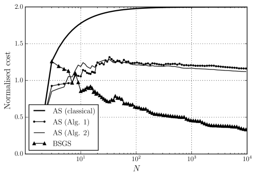
Figure 1: Normalized theoretical cost in the FFT model ($(3m+2.333s)/(3N)$ for $m$ complex multiplications and $s$ complex squarings) to add the first $N$ nonzero terms in the $q$-series of the Dedekind eta function, using three different addition sequences (AS) or the baby-step giant-step algorithm (BSGS). The classical addition sequences approaches $2$ multiplications per term. The short addition sequences generated with Algorithm 1 and Algorithm 2 both approach $1$ multiplication per term. BSGS is asymptotically better than any addition sequence.

6 Benchmarks

We have implemented the Jacobi theta functions and the Dedekind eta function in the Arb library [28], and complemented the existing implementation of the Dedekind eta function in release 0.3 of CM [14] by the baby-step giant-step algorithm. The complete function evaluation involves three steps:

1. Reduce $\tau\in\mathbb{C},\Im(\tau)>0$ to the fundamental domain of the action of $\operatorname{Sl}_{2}(\mathbb{Z})$ on the upper complex half-plane.

2. Compute $q=\exp(2\pi i\tau)$ (for $\eta$) or $q=\exp(\pi i\tau)$ (for $\vartheta_{i}$).

3. Sum the truncated $q$-series.

The first step has negligible cost. For the third step, we have implemented the optimized addition sequences (AS) as well as the baby-step giant-step (BSGS) algorithm. AS and BSGS are used automatically at low and high precision, respectively. Here, we compare both methods. The measurements were done on an Intel Core i5-4300U CPU running a 64-bit Linux kernel. MPIR 2.7.2 [25] was used for multiprecision arithmetic. Tables 7, 8 and 9 show timings with Arb, and Table 10 compares old implementations with the new implementations in Arb and CM.

We take $\tau=(-B+\sqrt{D})/(2A)$ with $A=1305,B=1523,D=-6961631$, which is a typical complex multiplication point occurring in class polynomial construction. The magnitude $|q|\approx 0.00174$ is slightly smaller than the worst case $|q|\approx 0.00433$ at the corner of the fundamental domain. For $p$ bits of floating point precision, the truncation order is $T\approx 0.11p$ when computing the eta function and $T\approx 0.22p$ when computing theta functions.

Our code includes a small practical optimization: For a tolerance of $2^{-p}$, the term $q^{n}$ needs to be computed to a precision of only $p-n|\log_{2}(|q|)|$ bits, and we change the internal precision for each term accordingly. Empirically, this saves roughly a factor of $1.5$ when using addition sequences and a factor of $1.2$ in the BSGS algorithm (which is improved less since the baby-steps have to be done at essentially full precision). The speed-up of the BSGS algorithm compared to addition sequences is therefore somewhat smaller than what one might predict by counting multiplications.

Bits	$T$	Exponential	Sum (AS)	Sum (BSGS)	Speed-up	Theory
$10^{2}$	7	$0.000\,001\,59$	$0.000\,001\,79$	$0.000\,002\,86$	0.63	0.74
$10^{3}$	100	$0.000\,018\,0$	$0.000\,026\,1$	$0.000\,023\,6$	1.11	1.34
$10^{4}$	1080	$0.001\,52$	$0.001\,69$	$0.001\,20$	1.41	1.63
$10^{5}$	10880	$0.066\,1$	$0.128$	$0.080\,9$	1.58	2.06
$10^{6}$	108676	$1.74$	$6.12$	$3.11$	1.97	2.32
$10^{7}$	1090987	$32.4$	$259$	$119$	2.18	2.77

Table 7: Timings for computing the Dedekind eta function at different precisions. From left to right: bit precision, truncation order $T$ (last included exponent), seconds to compute $q=\exp(2\pi i\tau)$, seconds to evaluate the sum using (AS), seconds to evaluate the sum using (BSGS), measured speed-up AS / BSGS, and theoretical speed-up based on counting multiplications in the FFT cost model.

Timings for the eta function are shown in Table 7. Here, AS is the optimized addition sequence of Algorithm 2. We time the complex exponential separately and only show the speed-up of (BSGS) over (AS) for the series summation. At lower precision, the complex exponential takes a comparable amount of time to summing the series, making the real-world speed-up smaller. The speed-up for the series summation by itself is nonetheless useful since there are situations where $q$ is available without the need to compute the full complex exponential, for example, during batch evaluation over an arithmetic progression of $\tau$ values.

Bits	$T$	Sum (AS)	Sum (BSGS)	Speed-up	Theoretical
$10^{2}$	20	$0.000\,003\,50$	$0.000\,005\,80$	0.60	0.67
$10^{3}$	210	$0.000\,038\,6$	$0.000\,049\,2$	0.78	0.89
$10^{4}$	2162	$0.002\,29$	$0.002\,16$	1.06	1.18
$10^{5}$	21756	$0.178$	$0.134$	1.33	1.55
$10^{6}$	218089	$8.97$	$5.71$	1.57	1.78
$10^{7}$	2181529	$380$	$199$	1.91	2.18

Table 8: Time in seconds to compute the theta functions $\vartheta_{0}(\tau),\vartheta_{1}(\tau),\vartheta_{2}(\tau)$ simultaneously, given $q=e^{\pi i\tau}$. Timings to compute the complex exponential are the same as in Table 7 and thus omitted.

Bits	$T$	Sum (AS)	Sum (BSGS)	Speed-up	Theoretical
$10^{2}$	16	$0.000\,002\,44$	$0.000\,003\,21$	0.76	0.84
$10^{3}$	196	$0.000\,031\,1$	$0.000\,024\,5$	1.27	1.51
$10^{4}$	2116	$0.001\,86$	$0.001\,10$	1.69	2.23
$10^{5}$	21609	$0.147$	$0.065\,3$	2.25	2.88
$10^{6}$	218089	$6.81$	$2.67$	2.55	2.95
$10^{7}$	2181529	$280$	$90.1$	3.11	3.58

Table 9: Time in seconds to compute $\vartheta_{0}(\tau)$ alone, given $q=e^{\pi i\tau}$. Timings to compute the complex exponential are the same as in Table 7 and thus omitted.

Table 8 shows the corresponding timings to compute three theta functions simultaneously. Here, AS uses Theorem 15, computing each term with one multiplication or squaring. The speed-up for BSGS is smaller compared to the eta function since three independent giant-step evaluations are done, one for each theta function. Table 9 shows timings for computing a single theta function. For AS, we use Algorithm 1 to generate a short addition sequence for the squares alone. Here the BSGS algorithm gives the largest speed-up.

Finally, Table 10 compares the new implementations with three previous implementations for the evaluation of $\eta(\tau)$. The eta function in PARI/GP [2] uses the classical addition sequence without the precision trick. CM [14] in version 0.2.1 used an optimized addition sequence (Algorithm 2) without the precision trick. An implementation of the AGM method courtesy of Régis Dupont (unpublished, cf. [11]) is also tested. All implementations were linked against the same version 2.7.2 of MPIR for multiprecision arithmetic.

Bits	PARI/GP	CM-0.2.1	AGM	New CM-0.3	New Arb
$10^{4}$	$0.008\,69$	$0.004\,57$	$0.007\,89$	$0.002\,97$	$0.002\,72$
$10^{5}$	$0.654$	$0.284$	$0.245$	$0.164$	$0.147$
$10^{6}$	$29.9$	$10.9$	$6.78$	$4.77$	$4.85$
$10^{7}$	$1\,310$	$440$	$124$	$150$	$151$

Table 10: Time in seconds to compute $\eta(\tau)$.

In conclusion, we achieve a small but measurable speed-up. At practical precisions, the baby-step giant-step algorithm saves somewhat less than a factor of $2$ in running time over an optimized addition sequence, which itself saves a factor of $2$ over the widely used classical addition sequence. Using an optimized addition sequence instead of the classical addition sequence raises the crossover point between series evaluation and the AGM method from about $10^{4}$ bits to $10^{5}$ bits, while the baby-step giant-step method raises it further to about $10^{6}$ bits, very roughly. The exact crossover point will vary depending on the system, the libraries used for multiprecision arithmetic, the size of $|q|$ (a smaller value is more advantageous for series evaluation), and whether $q$ needs to be computed from $\tau$ by a full exponential evaluation.

7 Acknowledgments

This research was partially funded by ERC Starting Grant ANTICS 278537 and DFG Priority Project SPP 1489.

 

2010 Mathematics Subject Classification: Primary 11Y55; Secondary 11B83, 11F20.

Keywords: addition sequence, pentagonal number, theta function, Dedekind eta function, polynomial evaluation, baby-step giant-step algorithm

 

(Concerned with sequences A001318, A002620, A084848, A085635, and A182568.)

References

- [1] P. T. Bateman and R. A. Horn. A heuristic asymptotic formula concerning the distribution of prime numbers. Math. Comp., 16:363–367, 1962.
- [2] K. Belabas et al. PARI/GP. Bordeaux, 2.7.5 edition, November 2015. http://pari.math.u-bordeaux.fr/.
- [3] D. J. Bernstein. Fast multiplication and its applications. In Algorithmic Number Theory, volume 44, pages 325–384. MSRI Publications, 2008.
- [4] D. V. Chudnovsky and G. V. Chudnovsky. Approximations and complex multiplication according to Ramanujan. In Ramanujan Revisited, pages 375–472. Academic Press, 1988. Proceedings of the Centenary Conference, University of Illinois at Urbana-Champaign, June 1–5, 1987.
- [5] H. Cohen. Advanced Topics in Computational Number Theory, volume 193 of Graduate Texts in Mathematics. Springer-Verlag, 2000.
- [6] H. Cohen, G. Frey, R. Avanzi, C. Doche, T. Lange, K. Nguyen, and F. Vercauteren. Handbook of Elliptic and Hyperelliptic Curve Cryptography. Discrete mathematics and its applications. Chapman & Hall/CRC, 2006.
- [7] D. A. Cox. Primes of the Form — Fermat, Class Field Theory, and Complex Multiplication. John Wiley & Sons, 1989.
- [8] L. E. Dickson. History of the Theory of Numbers, volume III — Quadratic and Higher Forms. Carnegie Institution of Washington, 1923.
- [9] D. Dobkin and R. J. Lipton. Addition chain methods for the evaluation of specific polynomials. SIAM J. Comput., 9:121–125, 1980.
- [10] P. Downey, B. Leong, and R. Sethi. Computing sequences with addition chains. SIAM J. Comput., 10:638–646, August 1981.
- [11] R. Dupont. Fast evaluation of modular functions using Newton iterations and the AGM. Math. Comp., 80:1823–1847, 2011.
- [12] A. Enge. The complexity of class polynomial computation via floating point approximations. Math. Comp., 78:1089–1107, 2009.
- [13] A. Enge. Computing modular polynomials in quasi-linear time. Math. Comp., 78:1809–1824, 2009.
- [14] A. Enge. CM — Complex multiplication of elliptic curves. INRIA, 0.2.1 edition, March 2015. Distributed under GPL v2+, http://cm.multiprecision.org/.
- [15] A. Enge and F. Morain. Generalised Weber functions. Acta Arith., 164:309–341, 2014.
- [16] A. Enge and R. Schertz. Constructing elliptic curves over finite fields using double eta-quotients. J. Théor. Nombres Bordeaux, 16:555–568, 2004.
- [17] A. Enge and R. Schertz. Singular values of multiple eta-quotients for ramified primes. LMS J. Comput. Math., 16:407–418, 2013.
- [18] L. Euler. Letter to Goldbach, 23 August 1755. http://eulerarchive.maa.org/correspondence/letters/OO0887.pdf.
- [19] L. Euler. De numeris, qui sunt aggregata duorum quadratorum. Novi commentarii academiae scientiarum Petropolitanae, 4:3–40, 1758. English translation at http://eulerarchive.maa.org/pages/E228.html.
- [20] L. Euler. Demonstratio theorematis fermatiani omnem numerum primum formae esse summam duorum quadratorum. Novi commentarii academiae scientiarum Petropolitanae, 5:3–58, 1760. English translation at http://eulerarchive.maa.org/pages/E241.html.
- [21] L. Euler. Specimen de usu observationum in mathesi pura. Novi commentarii academiae scientiarum Petropolitanae, 6:185–230, 1761. http://eulerarchive.maa.org/pages/E241.html.
- [22] L. Euler. Evolutio producti infiniti etc. in seriem simplicem. Acta Academiae Scientiarum Imperialis Petropolitanae, 1780:47–55, 1783.
- [23] C. F. Gauß. Disquisitiones Arithmeticae. Gerh. Fleischer Jun., 1801.
- [24] E. Grosswald. Representations of Integers as Sums of Squares. Springer-Verlag, 1985.
- [25] W. Hart. MPIR – Multiple Precision Integers and Rationals, 2.7.2 edition, 2015. http://mpir.org/.
- [26] M. D. Hirschhorn. The number of representations of a number by various forms involving triangles, squares, pentagons and octagons. In Nayandeep Deka Baruah, Bruce C. Berndt, Shaun Cooper, Tim Huber, and Michael Schlosser, editors, Ramanujan Rediscovered, volume 14 of RMS Lecture Notes Series, pages 113–124, Mysore, 2009. Ramanujan Mathematical Society.
- [27] F. Johansson. Evaluating parametric holonomic sequences using rectangular splitting. In Proceedings of the 39th International Symposium on Symbolic and Algebraic Computation, ISSAC ‘14, pages 256–263, New York, NY, USA, 2014. ACM.
- [28] F. Johansson. Arb – C library for arbitrary-precision ball arithmetic. INRIA, 2.8.1 edition, 2015. http://arblib.org/.
- [29] D. E. Knuth. The Art of Computer Programming, volume 2: Seminumerical Algorithms. Addison-Wesley, 3rd edition, 1998.
- [30] A. M. le Gendre. Essai sur la Théorie des Nombres. Duprat, 1797. http://gallica.bnf.fr/ark:/12148/btv1b8626880r.
- [31] D. Mumford. Tata Lectures on Theta I. Birkhäuser, 1983.
- [32] D. Mumford. Tata Lectures on Theta II — Jacobian Theta Functions and Differential Equations. Birkhäuser, 1984.
- [33] D. Mumford. Tata Lectures on Theta III. Birkhäuser, 1991.
- [34] M. S. Paterson and L. J. Stockmeyer. On the number of nonscalar multiplications necessary to evaluate polynomials. SIAM J. Comput., 2:60–66, March 1973.
- [35] H. Rademacher. The Fourier coefficients of the modular invariant . Amer. J. Math., 60:501–512, 1938.
- [36] J. B. Rosser and L. Schoenfeld. Approximate formulas for some functions of prime numbers. Illinois J. Math., 6:64–94, 1962.
- [37] R. Schertz. Weber’s class invariants revisited. J. Théor. Nombres Bordeaux, 14:325–343, 2002.
- [38] D. M. Smith. Efficient multiple-precision evaluation of elementary functions. Math. Comp., 52:131–134, 1989.
- [39] H. Weber. Lehrbuch der Algebra, volume 3: Elliptische Funktionen und algebraische Zahlen. Vieweg, 2nd edition, 1908.