Predictive Inference Based on Markov Chain Monte Carlo Output

Abstract

In Bayesian inference, predictive distributions are typically in the form of samples generated via Markov chain Monte Carlo (MCMC) or related algorithms. In this paper, we conduct a systematic analysis of how to make and evaluate probabilistic forecasts from such simulation output. Based on proper scoring rules, we develop a notion of consistency that allows to assess the adequacy of methods for estimating the stationary distribution underlying the simulation output. We then provide asymptotic results that account for the salient features of Bayesian posterior simulators, and derive conditions under which choices from the literature satisfy our notion of consistency. Importantly, these conditions depend on the scoring rule being used, such that the choices of approximation method and scoring rule are intertwined. While the logarithmic rule requires fairly stringent conditions, the continuous ranked probability score (CRPS) yields consistent approximations under minimal assumptions. These results are illustrated in a simulation study and an economic data example. Overall, mixture-of-parameters approximations which exploit the parametric structure of Bayesian models perform particularly well. Under the CRPS, the empirical distribution function is a simple and appealing alternative option.

1 Introduction

Probabilistic forecasts are predictive probability distributions over quantities or events of interest. They implement an idea that was eloquently expressed already at the beginning of the 20th century in the context of meteorological prediction:

“It seems to me that the condition of confidence or otherwise forms a very important part of the prediction, and ought to find expression.”

(Cooke, 1906, pp. 23–24)

Despite this early acknowledgment of the importance of forecast uncertainty, constructing principled and realistic measures of the latter remains challenging in practice. In this context, a rapidly growing transdisciplinary literature uses Bayesian inference to produce posterior predictive distributions in a wide range of applications, including economic, ecological, and meteorological problems, among many others. Bayesian posterior predictive distributions naturally account for sources of uncertainty – such as unknown model parameters, or latent variables in state space models – that are not easily captured using frequentist methods; see, e.g., Clark (2005) for an ecological perspective.

Formally, posterior predictive distributions arise as mixture distributions with respect to the posterior distribution of the parameter vector. In the following, we assume that the parameter vector contains all quantities that are subject to Bayesian inference, including also latent state variables, for example. For a real-valued continuous quantity of interest, the posterior predictive distribution, $F_{0}$, can be represented by its cumulative distribution function (CDF) or the respective density. The posterior predictive CDF is then of the generic form

$$F_{0}(x)=\int_{\Theta}F_{c}(x\hskip 0.56905pt|\hskip 0.85358pt\theta)\,{\rm d}P_{\rm post}(\theta)$$ (1)

for $x\in\mathbb{R}$, where $P_{\rm post}$ is the posterior distribution of the parameter, $\theta$, over some parameter space, $\Theta$, and $F_{c}(\cdot\hskip 0.56905pt|\hskip 0.85358pt\theta)$ is the conditional predictive CDF when $\theta\in\Theta$ is the true parameter. Harris (1989) argues that predictive distributions of this form have appeal in frequentist settings as well. Often, the integral in (1) does not admit a solution in closed form, and so the posterior predictive CDF must be approximated or estimated in some way, typically using some form of Markov chain Monte Carlo (MCMC); see, e.g., Gelfand and Smith (1990) and Gilks et al. (1996).

Given a simulated sequence $(\theta_{i})_{i=1}^{m}$ of parameter values from $P_{\rm post}$, one approach, which we call the mixture-of-parameters (MP) technique, is to approximate $F_{0}$ by

$$\hat{F}_{m}^{\rm MP}(x)=\frac{1}{m}\sum_{i=1}^{m}F_{c}(x\hskip 0.56905pt|\hskip 0.85358pt\theta_{i}).$$ (2)

However, this method can be used only when the conditional distributions $F_{c}(\cdot\hskip 0.56905pt|\hskip 0.85358pt\theta)$ are available in closed form. An alternative route is to simulate a sequence $(X_{i})_{i=1}^{m}$ where $X_{i}\sim F_{c}(\cdot\hskip 0.56905pt|\hskip 0.85358pt\theta_{i})$, and to approximate $F_{0}$ based on this sample, using either nonparametric or parametric techniques. The most straightforward option is to estimate $F_{0}$ by the empirical CDF (ECDF),

$$\hat{F}_{m}^{\rm ECDF}(x)=\frac{1}{m}\sum_{i=1}^{m}\mathbbm{1}\{x\geq X_{i}\}.$$ (3)

Alternatively, one might employ a kernel density (KD) estimate of the posterior predictive density, namely,

$$\hat{f}_{m}^{\rm KD}(x)=\frac{1}{mh_{m}}\sum_{i=1}^{m}K\!\left(\frac{x-X_{i}}{h_{m}}\right)\!,$$ (4)

where $K$ is a kernel function, i.e., a symmetric, bounded, and square-integrable probability density, such as the Gaussian or the Epanechnikov kernel, and $h_{m}$ is a suitable bandwidth (Rosenblatt, 1956; Silverman, 1986). Finally, much extant work employs a Gaussian approximation (GA) to $F_{0}$, namely

$$\hat{F}_{m}^{\rm GA}(x)=\Phi\!\left(\frac{x-\hat{\mu}_{m}}{\hat{\sigma}_{m}}\right)\!,$$ (5)

where $\Phi$ is the CDF of the standard normal distribution, and $\hat{\mu}_{m}$ and $\hat{\sigma}_{m}$ are the empirical mean and standard deviation of the sample $(X_{i})_{i=1}^{m}$.

Following Rubin (1984) and Little (2006), it is now widely accepted that posterior predictive inference should be evaluated using frequentist principles, without prior information entering at the model evaluation stage. For the comparison and ranking of probabilistic forecasting methods one typically uses a proper scoring rule (Gneiting and Raftery, 2007) that assigns a numerical score or penalty based on the predictive CDF, $F$, or its density, $f$, and the corresponding realization, $y$, such as the logarithmic score (LogS; Good, 1952),

$$\text{LogS}(F,y)=-\log f(y),$$ (6)

or the continuous ranked probability score (CRPS; Matheson and Winkler, 1976),

$$\text{CRPS}(F,y)=\int_{\mathbb{R}}\left(F(z)-\mathbbm{1}\{z\geq y\}\right)^{2}{\rm d}z.$$ (7)

While the LogS and CRPS are the two most popular scoring rules in applications, they feature interesting conceptual differences which we discuss in Section 2.2. In practice, one finds and compares the mean score over an out-of-sample test set, and the forecasting method with the smaller mean score is preferred. Formal tests of the null hypothesis of equal predictive performance can be employed as well (Diebold and Mariano, 1995; Giacomini and White, 2006; Clark and McCracken, 2013; DelSole and Tippett, 2014).

Table 1 of the Online Supplement summarizes the use of evaluation techniques in recently published comparative studies of probabilistic forecasting methods that use Bayesian inference via MCMC. As shown in the table, the mixture-of-parameters technique has mainly been applied in concert with the logarithmic score, whereas the empirical CDF method can be used in conjunction with the CRPS only. However, to this date, there are few, if any, guidelines to support choices in Table 1 of the Online Supplement, and it is not clear how they affect practical model comparisons. The present paper provides a systematic analysis of this topic. We focus on the following questions. First, what defines reasonable choices of the approximation method and scoring rule? Second, under what conditions do extant choices from the literature satisfy this definition? Third, for a given scoring rule, how accurate are alternative approximation methods in practically relevant scenarios?

In studying these questions, our work is complementary to Gneiting and Raftery (2007) who develop the broader theory of scoring rules and portray their rich mathematical and decision theoretic structure. While Gneiting and Raftery (2007) mention simulated predictive distributions (see in particular their Section 4.2), the empirical literature surveyed in the Online Supplement has largely evolved after 2007, giving rise to the applied techniques that motivate the present paper.

We emphasize that the present study — and the use of scoring rules in general — concern the comparative assessment of two or more predictive models: The model with the smallest mean score is considered the most appropriate. Comparative assessment is essential in order to choose among a large number of specifications typically available in practice. This task is different from absolute assessment, which amounts to diagnosing possible misspecification, using the probability integral transform (Dawid, 1984; Diebold et al., 1998), posterior predictive checks (Gelman et al., 1996; Held et al., 2010; Gelman et al., 2014a, Chapter 6) and related methods.

The remainder of this paper is organized as follows. Section 2 introduces the notion of a consistent approximation to $F_{0}$. This formalizes the idea that, as the size of the simulated sample becomes larger and larger, and in terms of a given scoring rule, the approximation ought to perform as well as the unknown true forecast distribution. In Section 3 we provide theoretical justifications of approximation methods encountered in the literature. Sections 4 and 5 present simulation and empirical evidence on the performance of these methods, and Section 6 concludes with a discussion. Overall, our findings support the use of the mixture-of-parameters estimator at (2) in order to approximate the posterior predictive distribution of interest. If this estimator is unavailable, the ECDF estimator at (3) is a simple and appealing alternative. Technical material and supplementary analyses are deferred to Appendices A to E. The Online Supplement contains a bibliography of the pertinent applied literature and additional figures.

2 Formal Setting

In this section, we discuss the posterior predictive distribution in Bayesian forecasting, give a brief review of proper scoring rules and score divergences, and introduce the concept of a consistent approximation method based on MCMC output.

As discussed earlier, the posterior predictive cumulative distribution function (CDF) of a Bayesian forecasting model is given by

$$F_{0}(x)=\int_{\Theta}F_{c}(x\hskip 0.56905pt|\hskip 0.85358pt\theta)\,{\rm d}P_{\rm post}(\theta)$$

where $\theta\in\Theta$ is the parameter, $P_{\rm post}$ is the posterior distribution of the parameter, and $F_{c}(\cdot\hskip 0.56905pt|\hskip 0.85358pt\theta)$ is the predictive distribution conditional on a parameter value $\theta$; see, e.g., Greenberg (2013, p. 33) or Gelman et al. (2014a, p. 7). A generic Markov chain Monte Carlo (MCMC) algorithm designed to sample from $F_{0}$ can be sketched as follows.

• Fix $\theta_{0}\in\Theta$ at some arbitrary value.

• For $i=1,2,\ldots$ iterate as follows:

  • Draw $\theta_{i}\sim{\cal K}(\theta_{i}\hskip 0.56905pt|\hskip 0.56905pt\theta_{i-1})$, where $\cal K$ is a transition kernel that specifies the conditional distribution of $\theta_{i}$ given $\theta_{i-1}$.

  • Draw $X_{i}\sim F_{c}(\cdot\hskip 0.56905pt|\hskip 0.85358pt\theta_{i})$.

We assume throughout that the transition kernel $\mathcal{K}$ is such that the sequence $(\theta_{i})_{i=1,2,\ldots}$ is stationary and ergodic in the sense of Geweke (2005, Definition 4.5.5) with invariant distribution $P_{\rm post}$, as holds widely in practice (Craiu and Rosenthal, 2014). Importantly, stationarity and ergodicity of $(\theta_{i})_{i=1,2,\ldots}$ with invariant distribution $P_{\rm post}$ imply that $(X_{i})_{i=1,2,\ldots}$ is stationary and ergodic with invariant distribution $F_{0}$ (Genon-Catalot et al., 2000, Proposition 3.1).

This generic MCMC algorithm allows for two general options for estimating the posterior predictive distribution $F_{0}$ in (1), namely,

• Option A: Based on parameter draws $(\theta_{i})_{i=1}^{m}$,

• Option B: Based on a sample $(X_{i})_{i=1}^{m}$,

where $m$ typically is on the order of a few thousands or ten thousands. Alternatively, some authors, such as Krüger et al. (2017), generate, for each $i=1,\ldots,m$, independent draws $X_{ij}\sim F_{c}(\cdot\hskip 0.56905pt|\hskip 0.85358pt\theta_{i})$, where $j=1,\dots,J$; see also Waggoner and Zha (1999, Section III. B). The considerations below apply in this more general setting as well.

2.1 Approximation methods

In the case of Option A, the sequence $(\theta_{i})_{i=1}^{m}$ of parameter draws is used to approximate the posterior predictive distribution, $F_{0}$, by the mixture-of-parameters estimator $\hat{F}_{m}^{\rm MP}$ in (2). Under the assumption of ergodicity,

$$\hat{F}_{m}^{\rm MP}(x)=\frac{1}{m}\sum_{i=1}^{m}F_{c}(x\hskip 0.56905pt|\hskip 0.85358pt\theta_{i})\longrightarrow\int_{\Theta}F_{c}(x\hskip 0.56905pt|\hskip 0.85358pt\theta)\,{\rm d}P_{post}(\theta)=F_{0}(x)$$

for $x\in\mathbb{R}$. This estimator was popularized by Gelfand and Smith (1990, Section 2.2), based on earlier work by Tanner and Wong (1987), and is often called a conditional or Rao-Blackwellized estimator. The latter term hints at variance reduction that may result from conditioning on the parameter draws (see Theorem 4 below). We refer to $\hat{F}_{m}^{\rm MP}$ as the mixture-of-parameters (MP) estimator.

In the case of Option B, the sample $(X_{i})_{i=1}^{m}$ is employed to approximate the posterior predictive distribution $F_{0}$. Various methods for doing this have been proposed and used, including the empirical CDF of the sample, denoted $\hat{F}_{m}^{\rm ECDF}$ in (3), the kernel density estimator $\hat{f}_{m}^{\rm KD}$ in (4), and the Gaussian approximation $\hat{F}_{m}^{\rm GA}$ in (5). Approaches of this type incur ‘more randomness than necessary’, in that the simulation step to draw $(X_{i})_{i=1}^{m}$ can be avoided if Option A is used. That said, Option A requires full knowledge of the model specification, as the conditional distributions must be known in closed form in order to compute $\hat{F}_{m}^{\rm MP}$. There are situations where this is restrictive, e.g., when the task is to predict a nonlinear transformation of the original, possibly vector-valued predictand (see the setup in Feldmann et al. 2015, Section 6d for an example from meteorology). We emphasize, however, that the mixture-of-parameters estimator is readily available in the clear majority of applied examples that we encounter in our work.
The implementation of the approximation methods (based on either Option A or B) is typically straightforward, except for the case of kernel density estimation, for which we discuss implementation choices in Section 3.3.

2.2 Proper scoring rules and score divergences

Let $\Omega\subseteq\mathbb{R}$ denote the set of possible values of the quantity of interest, and let $\mathcal{F}$ denote a convex class of probability distributions on $\Omega$. A scoring rule is a function

$${\rm S}:\mathcal{F}\times\Omega\longrightarrow\mathbb{R}\cup\{\infty\}$$

that assigns numerical values to pairs of forecasts $F\in\mathcal{F}$ and observations $y\in\Omega$. We typically set $\Omega=\mathbb{R}$, but will occasionally restrict attention to compact subsets.

Throughout this paper, we define scoring rules to be negatively oriented, i.e., a lower score indicates a better forecast. A scoring rule is proper relative to $\mathcal{F}$ if the expected score

$${\rm S}(F,G)=\int_{\Omega}{\rm S}(F,y)\,{\rm d}G(y)$$

is minimized for $F=G$, i.e., if

$${\rm S}(G,G)\leq{\rm S}(F,G)$$

for all probability distributions $F,G\in\mathcal{F}$. It is strictly proper relative to the class $\mathcal{F}$ if, furthermore, equality implies that $F=G$. The score divergence associated with the scoring rule $S$ is given by

$$d_{{\rm S}}(F,G)={\rm S}(F,G)-{\rm S}(G,G).$$

Clearly, $d_{{\rm S}}(F,G)\geq 0$ for all $F,G\in\mathcal{F}$ is equivalent to propriety of the scoring rule ${\rm S}$, which is a critically important property in practice.

Table 1: Examples of proper scoring rules, along with the associated score divergence and natural domain, $\mathcal{F}$. For a probability distribution with CDF $F$, we write $\mu_{F}$ for its mean, $\sigma_{F}$ for its standard deviation, and $f$ for its density.

Scoring rule	${\rm S}(F,y)$	$d_{{\rm S}}(F,G)$	$\mathcal{F}$
Logarithmic score	$-\log f(y)$	$\textstyle\int g(z)\log\frac{g(z)}{f(z)}\,{\rm d}z$	$\mathcal{L}_{1}$
CRPS	$\int\,(F(z)-\mathbbm{1}\{z\geq y\})^{2}\,{\rm d}z$	$\int\,(F(z)-G(z))^{2}\,{\rm d}z$	$\mathcal{M}_{1}$
Dawid–Sebastiani score	$\log\sigma^{2}_{F}+\frac{(y-\mu_{F})^{2}}{\sigma^{2}_{F}}$	$\frac{\sigma^{2}_{G}}{\sigma^{2}_{F}}-\log\frac{\sigma^{2}_{G}}{\sigma^{2}_{F}}+\frac{(\mu_{F}-\mu_{G})^{2}}{\sigma^{2}_{F}}-1$	$\mathcal{M}_{2}$

Table 1 shows frequently used proper scoring rules, along with the associated score divergences and the natural domain. For any given scoring rule ${\rm S}$, the associated natural domain is the largest convex class of probability distributions $F$ such that ${\rm S}(F,y)$ is well-defined and finite almost surely under $F$. Specifically, the natural domain for the popular logarithmic score (LogS; eq. (6)) is the class $\mathcal{L}_{1}$ of the probability distribution with densities, and the respective score divergence is the Kullback-Leibler divergence. The logarithmic score is local (Bernardo, 1979), that is, it evaluates a predictive model based only on the density value at the realizing outcome. Conceptually, this means that the logarithmic score ignores the model’s predicted probabilities of events that could have happened but did not. For the continuous ranked probability score (CRPS; eq. (7)), the natural domain is the class $\mathcal{M}_{1}$ of the probability distributions with finite mean. The LogS and CRPS are both strictly proper relative to their respective natural domains. In contrast to the logarithmic score, the CRPS rewards predictive distributions that place mass close to the realizing outcome, a feature that is often called ‘sensitivity to distance’ (e.g. Matheson and Winkler, 1976, Section 2). While various authors have argued in favor of either locality or sensitivity to distance, the choice between these two contrasting features appears ultimately subjective. Finally, the natural domain for the Dawid–Sebastiani score (DSS; Dawid and Sebastiani, 1999) is the class $\mathcal{M}_{2}$ of the probability distributions with strictly positive, finite variance. This score is proper, but not strictly proper, relative to $\mathcal{M}_{2}$.

2.3 Consistent approximations

To study the combined effects of the choices of approximation method and scoring rule in the evaluation of Bayesian predictive distributions, we introduce the notion of a consistent approximation procedure.

Specifically, let $(\theta_{i})_{i=1,2,\ldots}$ or $(X_{i})_{i=1,2,\ldots}$, where $X_{i}\sim F_{c}(\cdot\hskip 0.56905pt|\hskip 0.85358pt\theta_{i})$, be output from a generic MCMC algorithm with the following property.

• The process $(\theta_{i})_{i=1,2,\ldots}$ is stationary and ergodic with invariant distribution $P_{\rm post}$.

As noted, assumption (A) implies that $(X_{i})_{i=1,2,\ldots}$ is stationary and ergodic with invariant distribution $F_{0}$. Consider an approximation method that produces, for all sufficiently large positive integers $m$, an estimate $\hat{F}_{m}$ that is based on $(\theta_{i})_{i=1}^{m}$ or $(X_{i})_{i=1}^{m}$, respectively. Let ${\rm S}$ be a proper scoring rule, and let $\mathcal{F}$ be the associated natural domain. Then the approximation method is consistent relative to the scoring rule ${\rm S}$ at the distribution $F_{0}\in\mathcal{F}$ if $\hat{F}_{m}\in\mathcal{F}$ for all sufficiently large $m$, and

$$d_{{\rm S}}(\hat{F}_{m},F_{0})\longrightarrow 0$$

or, equivalently, ${\rm S}(\hat{F}_{m},F_{0})\to{\rm S}(F_{0},F_{0})$ almost surely as $m\to\infty$. This formalizes the idea that under continued MCMC sampling, the approximation ought to perform as well as the unknown true posterior predictive distribution. We contend that this is a highly desirable property in practical work.

Note that $\hat{F}_{m}$ is a random quantity that depends on the sample $(\theta_{i})_{i=1}^{m}$ or $(X_{i})_{i=1}^{m}$. The specific form of the divergence stems from the scoring rule, which mandates convergence of a certain functional of the estimator or approximation, $\hat{F}_{m}$, and the theoretical posterior predictive distribution, $F_{0}$. As we will argue, this aspect has important implications for the choice of scoring rule and approximation method.

Our concept of a consistent approximation procedure is independent of the question of how well a forecast model represents the ‘true’ uncertainty. The definition thus allows to separate the problem of interest, namely, to find a good approximation $\hat{F}_{m}$ to $F_{0}$, from the distinct task of finding a good probabilistic forecast $F_{0}$. We further emphasize that we study convergence in the sample size, $m$, of MCMC output, given a fixed number of observations, say, $T$, used to fit the model. Our analysis is thus distinct from traditional Bayesian asymptotic analyses that study convergence of the posterior distribution as $T$ becomes larger and larger (see, e.g., Gelman et al., 2014a, Section 4), thereby calling for markedly different technical tools.

2.4 Relation to total variation and Wasserstein distances

Our focus on score divergences (in particular, on $d_{\text{LogS}}$ and $d_{\text{CRPS}}$) is motivated by their natural relation to scoring rules, which in turn are popular tools in the applied literature on probabilistic forecasting. As reviewed by Gibbs and Su (2002), many other distance metrics for comparing two probability distributions have been proposed in the literature. Among these metrics, the total variation distance ($d_{\textnormal{TV}}$) has received much attention in theoretical work on MCMC (e.g. Tierney, 1994; Rosenthal, 1995), and is thus particularly relevant in our context. The total variation distance between two absolutely continuous probability measures with densities $f$ and $g$ is defined as

$$d_{\textnormal{TV}}(F,G)=\frac{1}{2}\int_{-\infty}^{\infty}|f(z)-g(z)|\,{\rm d}z.$$

As $2\hskip 0.56905ptd_{\textnormal{TV}}(F,G)^{2}\leq d_{\text{LogS}}(F,G)$ (e.g., Barron et al., 1992), convergence in terms of $d_{\text{LogS}}$ implies convergence in terms of $d_{\textnormal{TV}}$.

The Wasserstein distance is a divergence function motivated by optimal transport problems (Villani, 2008) and has received much attention in statistics and machine learning (Panaretos and Zemel, 2019). Here, we limit our discussion to the Wasserstein distance of order 1, which is most common in practice, and denote the corresponding metric by

$$d_{\textnormal{W}}(F,G)=\int_{0}^{1}|F^{-1}(\alpha)-G^{-1}(\alpha)|\,{\rm d}\alpha=\int_{-\infty}^{\infty}|F(z)-G(z)|\,{\rm d}z,$$

where $F^{-1}$ and $G^{-1}$ are the quantile functions of $F$ and $G$ respectively. Bellemare et al. (2017) discuss shortcomings of Wasserstein distances in estimation with stochastic gradient descent methods and suggest $d_{\text{CRPS}}$ as a superior alternative. This recommendation relates to the observation that there is no proper scoring rule with $d_{\textnormal{W}}$ as score divergence (Thorarinsdottir et al., 2013, Theorem 2).

As $d_{\text{CRPS}}(F,G)\leq d_{\textnormal{W}}(F,G)$, convergence in terms of $d_{\textnormal{W}}$ implies convergence in terms of $d_{\text{CRPS}}$. If $F$ and $G$ have densities with support in a common interval of length $l$, $d_{\textnormal{W}}(F,G)\leq l\cdot d_{\textnormal{TV}}(F,G)\leq l\cdot\sqrt{d_{\text{LogS}}(F,G)/2}$, so in this case consistency relative to the logarithmic score implies consistency relative to the CRPS. For further relations to the Kolmororov, Lévy, Prohorov and bounded Lipschitz distances see Section 2.4 of Huber and Ronchetti (2009).

3 Consistency results and computational complexity

Table 2: Upper bounds on the computational complexity of approximation methods in terms of the size $m$ of the MCMC sample $(\theta_{i})_{i=1}^{m}$ or $(X_{i})_{i=1}^{m}$, respectively, for pre-processing, and for the exact computation of the CRPS, Dawid–Sebastiani score (DSS) and logarithmic score (LogS).

Approximation method	Pre-processing	CRPS	DSS	LogS
MP	${\cal O}(1)$	${\cal O}(m^{2})$	${\cal O}(m^{2})$	${\cal O}(m)$
ECDF	${\cal O}(1)$	${\cal O}(m\log m)$	${\cal O}(m)$
KD	${\cal O}(m)$	${\cal O}(m^{2})$	${\cal O}(m)$	${\cal O}(m)$
Gaussian	${\cal O}(m)$	${\cal O}(1)$	${\cal O}(1)$	${\cal O}(1)$

We now investigate sufficient conditions for consistency of the aforementioned approximation methods, namely, the mixture-of-parameters (MP) estimator $\hat{F}_{m}^{\rm MP}$ in (2), the empirical CDF (ECDF) method $\hat{F}_{m}^{\rm ECDF}$ in (3), the kernel density (KD) estimate $\hat{f}_{m}^{\rm KD}$ in (4), and the Gaussian approximation (GA) $\hat{F}_{m}^{\rm GA}$ in (5). Table 2 summarizes upper bounds on the computational cost of pre-processing and computing the CRPS, Dawid–Sebastiani score (DSS) and logarithmic score (LogS) under these methods in terms of the size $m$ of the MCMC sample $(\theta_{i})_{i=1}^{m}$ or $(X_{i})_{i=1}^{m}$, respectively.

Consistency requires the convergence of some functional of the approximation, $\hat{F}_{m}$, and the true posterior predictive distribution, $F_{0}$. The conditions to be placed on the Bayesian model $F_{0}$, the estimator $\hat{F}_{m}$, and the dependence structure of the MCMC output depend on the scoring rule at hand.

3.1 Mixture-of-parameters estimator

We now establish consistency of the mixture-of-parameters estimator $\hat{F}_{m}^{\rm MP}$ in (2) relative to the CRPS, DSS and logarithmic score. The proofs are deferred to Appendix B.

Theorem 1 (consistency of mixture-of-parameters approximations relative to the CRPS and DSS). Under assumption (A), the mixture-of-parameters approximation is consistent relative to the CRPS at every distribution $F_{0}$ with finite mean, and consistent relative to the DSS at every distribution $F_{0}$ with strictly positive, finite variance.

Theorem 1 is the best possible result of its kind: It applies to every distribution in the natural domain and does not invoke any assumptions on the Bayesian model. In contrast, Theorem 2 hinges on rather stringent further conditions on the distribution $F_{0}$ and the Bayesian model (1), as follows.

• The distribution $F_{0}$ is supported on some bounded interval $\Omega$. It admits a density, $f_{0}$, that is continuous and strictly positive on $\Omega$. Furthermore, the density $f_{c}(\cdot\hskip 0.56905pt|\hskip 0.85358pt\theta)$ is continuous for every $\theta\in\Theta$.

Theorem 2 (consistency of mixture-of-parameters approximations relative to the logarithmic score). Under assumptions (A) and (B), the mixture-of-parameters approximation is consistent relative to the logarithmic score at the distribution $F_{0}$.

While we believe that the mixture-of-parameters technique is consistent under weaker assumptions, this is the strongest result that we have been able to prove. In particular, condition (B) does not allow for the case $\Omega=\mathbb{R}$. However, practical applications often involve a truncation of the support for numerical reasons, as exemplified in Section 4, and in this sense the assumption may not be overly restrictive.

Computing the logarithmic score and the DSS for a predictive distribution $\hat{F}_{m}^{\rm MP}$ of the form (2) is straightforward. To compute the CRPS, we note from eq. (21) of Gneiting and Raftery (2007) that

$$\text{CRPS}\left(\hat{F}_{m}^{\rm MP},y\right)=\frac{1}{m}\sum_{i=1}^{m}\mathbb{E}|Z_{i}-y|-\frac{1}{2m^{2}}\sum_{i=1}^{m}\sum_{j=1}^{m}\mathbb{E}|Z_{i}-Z_{j}|,$$ (8)

where $Z_{i}$ and $Z_{j}$ are independent random variables with distribution $F_{c}(\cdot\hskip 0.56905pt|\hskip 0.85358pt\theta_{i})$ and $F_{c}(\cdot\hskip 0.56905pt|\hskip 0.85358pt\theta_{j})$, respectively. The expectations on the right-hand side of (8) often admit closed form expressions that can be derived with techniques described by Jordan (2016) and Taillardat et al. (2016), including but not limited to the ubiquitous case of Gaussian variables. Then the evaluation requires ${\cal O}(m^{2})$ operations, as reported in Table 2. In Appendix A, we provide details and investigate the use of numerical integration in (7), which provides an attractive, computationally efficient alternative.

3.2 Empirical CDF-based approximation

The empirical CDF-based approximation $\hat{F}_{m}^{\rm ECDF}$ in (3), which builds on a simulated sample $(X_{i})_{i=1}^{m}$, is consistent relative to the CRPS and DSS under minimal assumptions. We prove the following result in Appendix C, which is the best possible of its kind, as it applies to every distribution in the natural domain and does not invoke any assumptions on the Bayesian model.

Theorem 3 (consistency of empirical CDF-based approximations relative to the CRPS and DSS). Under assumption (A), the empirical CDF technique is consistent relative to the CRPS at every distribution $F_{0}$ with finite mean, and consistent relative to the DSS at every distribution $F_{0}$ with strictly positive, finite variance.

As stated in Table 2, the computation of the CRPS under $\hat{F}_{m}^{\rm ECDF}$ requires $\mathcal{O}(m\log{}m)$ operations only. Specifically, let $X_{(1)}\leq\cdots\leq X_{(m)}$ denote the order statistics of $X_{1},\ldots,X_{m}$, which can be obtained in $\mathcal{O}(m\log{}m)$ operations. Then

$$\text{CRPS}\left(\hat{F}_{m}^{\rm ECDF},y\right)=\frac{2}{m^{2}}\sum_{i=1}^{m}(X_{(i)}-y)\left(m\mathbbm{1}\{y<X_{(i)}\}-i+\frac{1}{2}\right)\!;$$ (9)

see Jordan (2016, Section 6) for details. A special case of eq. (8) suggests another way of computing the CRPS, in that

$$\text{CRPS}\left(\hat{F}_{m}^{\rm ECDF},y\right)=\frac{1}{m}\sum_{i=1}^{m}|X_{i}-y|-\frac{1}{2m^{2}}\sum_{i=1}^{m}\sum_{j=1}^{m}|X_{i}-X_{j}|.$$ (10)

The representations in (9) and (10) are algebraically equivalent, but the latter requires $\mathcal{O}(m^{2})$ operations and thus is inefficient.

While the consistency results support the use of both $\hat{F}_{m}^{\rm MP}$ and $\hat{F}_{m}^{\rm ECDF}$, Rao-Blackwellization arguments indicate superiority of $\hat{F}_{m}^{\rm MP}$.

Theorem 4 (comparison of $\hat{F}_{m}^{\rm MP}$ and $\hat{F}_{m}^{\rm ECDF}$). Under assumption (A), $\mathbb{E}\,\hat{F}_{m}^{\rm MP}(z)=\mathbb{E}\,\hat{F}_{m}^{\rm ECDF}(z)$ and $\textnormal{Var}\,\hat{F}_{m}^{\rm MP}(z)\leq\textnormal{Var}\,\hat{F}_{m}^{\rm ECDF}(z)$ for any $z\in\Omega$ and $m\in\mathbb{N}$. If furthermore $F_{0}$ has finite mean, then $\mathbb{E}\,d_{\textnormal{CRPS}}\left(\hat{F}_{m}^{\rm MP},F_{0}\right)\leq\mathbb{E}\,d_{\textnormal{CRPS}}\left(\hat{F}_{m}^{\rm ECDF},F_{0}\right)$ for any $m\in\mathbb{N}$.

Theorem 4 demonstrates that $\hat{F}_{m}^{\rm MP}$ outperforms $\hat{F}_{m}^{\rm ECDF}$ in terms of expected divergence, for every given sample size $m$. Proposition 5 of Bolin and Wallin (2020) shows that if $F_{0}$ is a normal location-scale mixture then the CRPS under the mixture-of-parameters estimator additionally has smaller variance than under the empirical CDF-based approximation.

Despite the theoretical superiority of $\hat{F}_{m}^{\rm MP}$, $\hat{F}_{m}^{\rm ECDF}$ may be attractive in practice, especially if the conditional distributions $F_{c}(\cdot|\theta)$ underlying $\hat{F}_{m}^{\rm MP}$ are difficult to compute analytically. For example, this may occur if the predictand $Y$ is modeled only indirectly (such as when $Y$ is the maximal element of a vector valued random variable).

3.3 Kernel density estimator

We now discuss conditions for the consistency of the kernel density estimator $\hat{f}_{m}^{\rm KD}$. In the present case of dependent samples $(X_{i})_{i=1}^{m}$, judicious choices of the bandwidth $h_{m}$ in (4) require knowledge of dependence properties of the sample, and the respective conditions are difficult to verify in practice.

The score divergence associated with the logarithmic score is the Kullback-Leibler divergence, which is highly sensitive to tail behavior. Therefore, consistency of $\hat{f}_{m}^{\rm KD}$ requires that the tail properties of the kernel $K$ in (4) and the true posterior predictive density $f_{0}$ be carefully matched, and any results tend to be technical (cf. Hall (1987)). Roussas (1988), Györfi et al. (1989), Yu (1993) and Liebscher (1996), among others, establish almost sure strong uniform consistency of $\hat{f}_{m}^{\rm KD}$ under $\alpha$- or $\beta$-mixing and other conditions. As noted in Appendix B, almost sure strong uniform consistency then implies consistency relative to the logarithmic score under assumption (B). Based on Hansen (2008) who proves general results we give conditions for consistency of the kernel density estimator $\hat{f}_{m}^{\rm KD}$, and summarize the relevant assumptions in the following condition.

• For the kernel function $K$, the bandwidth $h_{m}$, and the dependence properties of $(X_{i})_{i=1,2,\dots}$ assumptions 1–3 and the conditions of Theorem 7 of Hansen (2008) are satisfied.

Theorem 5 (consistency of kernel density estimator-based approximations relative to the LogS). Under assumptions (A), (B), and (H), the kernel density estimator-based approximation technique is consistent relative to the logarithmic score at the distribution $F_{0}$.

The result is a direct consequence of Hansen (2008, Theorem 7) who further provides optimal convergence rates. However, the respective conditions are stringent and difficult to check in practice. Indeed, Wasserman (2006, p. 57) opines that “Despite the natural role of Kullback-Leibler distance in parametric statistics, it is usually not an appropriate loss function in smoothing problems”.

Under the conditions of Theorem 5, consistency of $\hat{F}_{m}^{\rm KD}$ relative to the CRPS follows directly, see Section 2.4. Kernel density estimation approximations are generally not consistent relative to the DSS due to the variance inflation induced by typical choices of the bandwidth. However, adaptations based on rescaling or weighting allow for kernel density estimation under moment constraints, see, e.g., Jones (1991) and Hall and Presnell (1999).

As this brief review suggests, the theoretical properties of kernel density estimators depend on the specifics of both the MCMC sample and the estimator. However, under the CRPS and DSS, a natural alternative is readily available: The empirical CDF approach is simpler and computationally cheaper than kernel density estimation, and is consistent under weak assumptions (Theorem 3).

In our simulation and data examples, we use a simple implementation of kernel density estimator-based approximations based on the Gaussian kernel and the Silverman (1986) plug-in rule for bandwidth selection. This leads to the specific form

$$\hat{F}_{m}^{\rm KD}(x)=\frac{1}{m}\sum_{i=1}^{m}\Phi\!\left(\frac{x-X_{i}}{h_{m}}\right)\!,$$ (11)

where $\Phi$ denotes the CDF of the standard normal distribution, and

$$h_{m}=1.06\leavevmode\nobreak\ \hat{A}_{m}\,m^{-1/5},$$ (12)

where $\hat{A}_{m}=\text{min}(\hat{\sigma}_{m},\frac{\text{IQR}_{m}}{1.34})$ is the minimum of the standard deviation and the (scaled) interquartile range $\text{IQR}_{m}$ of $(X_{i})_{i=1}^{m}$. The pre-processing costs of the procedure are ${\cal O}(m)$, as shown in Table 2. This choice of $h_{m}$, which is implemented in the R function bw.nrd (R Core Team, 2019), is motivated by simulation evidence in Hall et al. (1995). Using the Sheather and Jones (1991) rule or cross-validation based methods yields slightly inferior results in our experience.

3.4 Gaussian approximation

A parametric approximation method fits a member of a fixed parametric family, say $\mathcal{F}_{\Gamma}$, of probability distributions to the MCMC sample $(X_{i})_{i=1}^{m}$. The problem of estimating the unknown distribution $F_{0}$ is thus reduced to a finite-dimensional parameter estimation problem. The most important case is the quadratic or Gaussian approximation, which takes $\mathcal{F}_{\Gamma}$ to be the Gaussian family, so that

$$\hat{F}_{m}^{\rm GA}(x)=\Phi\!\left(\frac{x-\hat{\mu}_{m}}{\hat{\sigma}_{m}}\right)\!,$$

where $\hat{\mu}_{m}$ and $\hat{\sigma}_{m}$ are the empirical mean and standard deviation of $(X_{i})_{i=1}^{m}$. If $F_{0}$ has a density $f_{0}$ that is unimodal and symmetric, the approximation can be motivated by a Taylor series expansion of the log predictive density at the mode, similar to Gaussian approximations of posterior distributions in large-sample Bayesian inference (e.g. Kass and Raftery, 1995; Gelman et al., 2014a, Chapter 4).

If $F_{0}$ is not Gaussian, $\hat{F}_{m}^{\rm GA}$ fails to be consistent relative to the logarithmic score and CRPS. However, the Ergodic Theorem implies that the Gaussian approximation is consistent relative to the Dawid–Sebastiani score under minimal conditions.

Theorem 6 (consistency of Gaussian approximations relative to the DSS). Under assumption (A), the Gaussian approximation technique is consistent relative to the DSS at every distribution $F_{0}$ with strictly positive, finite variance.

We also note that the logarithmic score for the Gaussian approximation $\hat{F}_{m}^{\rm GA}$ corresponds to the Dawid–Sebastiani score for the empirical CDF-based approximation $\hat{F}_{m}^{\rm ECDF}$, in that

$$\text{LogS}\!\left(\hat{F}_{m}^{\rm GA},y\right)=\frac{1}{2}\left(\log 2\pi+\text{DSS}\!\left(\hat{F}_{m}^{\rm ECDF},y\right)\right)$$

for $y\in\mathbb{R}$. Therefore, the Gaussian approximation under the logarithmic score yields model rankings that are identical to those for the empirical CDF technique under the Dawid–Sebastiani score. From an applied perspective, this equivalence suggests that the inconsistency of the Gaussian approximation may not be overly problematic when the approximation is used in concert with the logarithmic score, an assessment that is in line with empirical findings by Warne et al. (2016). However, researchers should be aware of the fact that they are effectively using a proper, but not strictly proper, scoring rule (namely, the Dawid–Sebastiani score) that focuses on the first two moments of the predictive distribution only.

4 Simulation study

We now investigate the various approximation methods in a simulation study that is designed to emulate MCMC behavior with dependent samples. Here, the posterior predictive distribution $F_{0}$ is known by construction, and so we can compare the different approximations to the true forecast distribution. For simplicity, our choice of $F_{0}$ is fixed and does not correspond to a particular Bayesian model.

In order to judge the quality of an approximation $\hat{F}_{m}$ of $F_{0}$ we consider the score divergence $d_{{\rm S}}(\hat{F}_{m},F_{0})$. Note that $d_{{\rm S}}(\hat{F}_{m},F_{0})$ is a random variable, since $\hat{F}_{m}$ depends on the particular MCMC sample $(\theta_{i})_{i=1}^{m}$ or $(X_{i})_{i=1}^{m}$. In our results below, we therefore consider the distribution of $d_{{\rm S}}(\hat{F}_{m},F_{0})$ across repeated simulation runs. For a generic approximation method producing an estimate $\hat{F}_{m}$, we proceed as follows:

• For simulation run $k=1,\dots,K$:

  • Draw MCMC samples $(\theta_{i}^{(k)})_{i=1}^{m}$ and $(X_{i}^{(k)})_{i=1}^{m}$

  • Compute the approximation $\hat{F}_{m}^{(k)}$ and the divergence $d_{{\rm S}}(\hat{F}_{m}^{(k)},F_{0})$ for the approximation methods and scoring rules under consideration.

• For each approximation method and scoring rule, summarize the distribution of
  $d_{{\rm S}}(\hat{F}_{m}^{(1)},F_{0}),\ldots,d_{{\rm S}}(\hat{F}_{m}^{(K)},F_{0})$.

In order to simplify notation, we typically suppress the superscript that identifies the Monte Carlo iteration. The results below are based on $K=1\,000$ replicates.

4.1 Data generating process

We generate sequences $(\theta_{i})_{i=1}^{m}$ and $(X_{i})_{i=1}^{m}$ in such a way that the invariant distribution,

$$F_{0}(x)=\int_{(0,\infty)}\Phi\!\left(\frac{x}{\theta}\right){\rm d}H_{0}(\theta^{2}),$$

where $\Phi$ denotes the standard normal CDF, is a compound Gaussian distribution or normal scale mixture. Depending on the measure $H_{0}$, which assumes the role of the posterior distribution $P_{\rm post}$ in the general Bayesian model (1), $F_{0}$ can be modeled flexibly, including many well-known parametric distributions (Gneiting, 1997). As detailed below, our choice of $H_{0}$ implies that

$$F_{0}(x)=\textsf{T}\left(x\,\bigg{|}\,0,\frac{ns}{n+2},n+2\right)\;$$ (13)

where $\textsf{T}(\cdot|a,b,c)$ denotes the CDF of a variable $Z$ with the property that $(Z-a)/\sqrt{b}$ is standard Student $t$ distributed with $c$ degrees of freedom. To mimic a realistic MCMC scenario with dependent draws, we proceed as proposed by Fox and West (2011). Given parameter values $n>0$, $s>0$ and $\alpha\in(-1,1)$, let

$$\psi_{i} \sim\text{IG}\!\left(\frac{1}{2}\,(n+3),\frac{1}{2}\,ns(1-\alpha^{2})\right)\!,$$ (14)

$$\upsilon_{i}\,|\,\psi_{i} \sim\mathcal{N}\!\left(\alpha,\frac{\psi_{i}}{ns}\right)\!,$$ (15)

$$\theta_{i}^{2} =\psi_{i}+\upsilon_{i}^{2}\,\theta_{i-1}^{2},\rule{0.0pt}{17.07164pt}$$ (16)

$$X_{i}\,|\,\theta_{i}^{2} \sim\mathcal{N}(0,\theta_{i}^{2})\rule{0.0pt}{19.91692pt}$$ (17)

where IG is the Inverse Gamma distribution, parametrized such that $Z\sim\text{IG}(a,b)$ when $1/Z\sim\text{G}(a,b)$, with G being the Gamma distribution with shape $a\geq 0$ and rate $b>0$.

Table 3: Hyper-parameters for the data generating process in the simulation setting of equations (14) to (17).

Parameter	Main role	Value(s) considered
$\alpha$	Persistence of $\theta_{i}^{2}$	{0.1, 0.5, 0.9}
$s$	Unconditional mean of $\theta_{i}^{2}$	2
$n$	Unconditional variance of $\theta_{i}^{2}$	{12, 20}

Table 3 summarizes our choices for the parameter configurations of the data generating process. The parameter $\alpha$ determines the persistence of the chain, in that the unconditional mean of $\upsilon_{i}^{2}$, which can be viewed as an average autoregressive coefficient (Fox and West, 2011, Section 2.3), is given by $(n\alpha^{2}+1)/(n+1)$. We consider three values, aiming to mimic MCMC chains with different persistence properties. The parameter $s$ represents a scale effect, and $n$ governs the tail thickness of the unconditional Student $t$ distribution in (13). We consider values of 12 and 20 that seem realistic for macroeconomic variables, such as the growth rate of the gross domestic product, that feature prominently in the empirical literature.

4.2 Approximation methods

We consider the following approximation methods, which have been discussed in detail in Section 3. The first approximation uses a sequence $(\theta_{i})_{i=1}^{m}$ of parameter draws, and the other three employ an MCMC sample $(X_{i})_{i=1}^{m}$.

• Mixture-of-parameters estimator $\hat{F}_{m}^{\rm MP}$ in (2), which here is of the form

  $$\hat{F}_{m}^{\rm MP}(x)=\frac{1}{m}\sum_{i=1}^{m}\Phi\!\left(\frac{x}{\theta_{i}}\right)\!,$$

  where $\theta_{i}$ is the predictive standard deviation drawn in MCMC iteration $i$.

• Empirical CDF-based approximation $\hat{F}_{m}^{\rm ECDF}$ in (3).

• The nonparametric kernel density estimator $\hat{f}_{m}^{\rm KD}$ using a Gaussian kernel and the Silverman rule for bandwidth selection, with predictive CDF $\hat{F}_{m}^{\rm KD}$ of the form (11).

• Gaussian approximation $\hat{F}_{m}^{\rm GA}$ in (5).

It is interesting to observe that here $\hat{F}_{m}^{\rm MP}$ is a scale mixture of centered Gaussian distributions, and $\hat{F}_{m}^{\rm KD}$ is a location mixture of normal distributions, whereas the quadratic approximation $\hat{F}_{m}^{\rm GA}$ is a single Gaussian.

The conditions for consistency of the mixture-of-parameters and empirical CDF approximations relative to the CRPS in Theorems 1 and 3 are satisfied. Furthermore, one might argue that numerically the support of $F_{0}$ and $\hat{F}_{m}^{\rm MP}$ is bounded (cf. below), and then the assumptions of Theorem 2 also are satisfied. Clearly, the Gaussian approximation fails to be consistent relative to the CRPS or the logarithmic score, as $F_{0}$ is not Gaussian.

For each approximation method, scoring rule ${\rm S}$, sample size $m$ and replicate $k$, we evaluate the score divergence $d_{{\rm S}}(\hat{F}_{m}^{(k)},F_{0})$. The divergence takes the form of a univariate integral (cf. Table 1) that is not available in closed form. Therefore, we compute $d_{{\rm S}}(\hat{F}_{m}^{(k)},F_{0})$ by numerical integration as implemented in the R function integrate. This is unproblematic if the scoring rule is the CRPS. For the logarithmic score, the integration is numerically challenging, as the logarithm of the densities needs to be evaluated in their tails. We therefore truncate the support of the integral to the minimal and maximal values that yield numerically finite values of the integrand.

4.3 Main results

Logarithmic score	CRPS

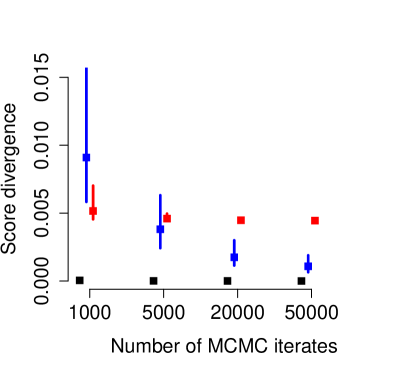
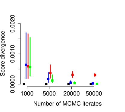
Figure 1: Score divergences in the simulation study with $(\alpha,s,n)=(0.5,2,12)$. For a given method and MCMC sample size, the bars range from the 10th to the 90th percentile of the score divergences across 1 000 replicates. The squares mark the respective medians.

Logarithmic score	CRPS

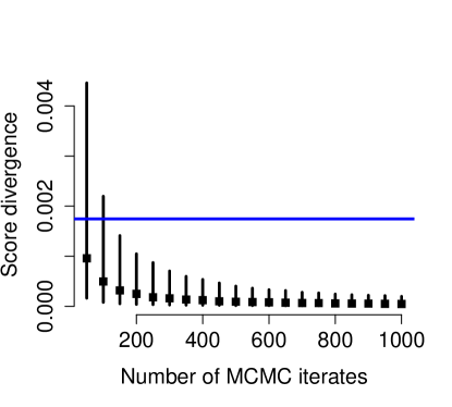
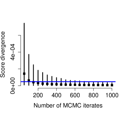
Figure 2: Performance of the mixture-of-parameters estimator. The design is as in Figure 1, but for smaller sample sizes. For comparison, the blue horizontal line marks the median divergence of the kernel density estimator based on 20 000 draws.

In the interest of brevity, we restrict attention to results for a single set of parameters of the data generating process, namely $(\alpha,s,n)=(0.5,2,12)$. This implies an unconditional Student $t$ distribution with 14 degrees of freedom, and intermediate autocorrelation of the MCMC draws. The results for the other parameter constellations in Table 3 are similar and available in the Online Supplement.

Figure 1 illustrates the performance of the approximation methods under the logarithmic score and the CRPS, by showing the distribution of the score divergence $d_{{\rm S}}(\hat{F}_{m},F_{0})$ as the sample size $m$ grows. The mixture-of-parameters estimator dominates the other methods by a wide margin: Its divergences are very close to zero, and show little variation across replicates. Under the logarithmic score, the performance of the kernel density estimator is highly variable across the replicates, even for large sample sizes. The variability is less under the CRPS, where the kernel density approach using the Silverman (1986) rule of thumb for bandwidth selection performs similar to the empirical CDF-based approximation. Other bandwidth selection rules we have experimented with tend to be inferior, as indicated by slower convergence and higher variability across replicates. Finally, we observe the lack of consistency of the Gaussian approximation.

Figure 2 provides insight into the performance of the mixture-of-parameters approximation for small MCMC samples. Using as few as 150 draws, the method attains a lower median CRPS divergence than the kernel density estimator based on 20 000 draws. The superiority of the mixture-of-parameters estimator is even more pronounced under the logarithmic score, where only 50 draws are required to outperform the kernel density estimator based on 20 000 draws.

4.4 Thinning the MCMC Sample

In Appendix D, we present simulation analyses of the effects of thinning an MCMC sample (i.e., keeping only every $\tau$th draw, where $\tau\in\mathbb{N}$ is the thinning factor), which is often done in practice with the goal of reducing autocorrelation in the MCMC draws. From a practical perspective, the analysis in Appendix D suggests that thinning is justified if, and only if, a small MCMC sample is desired and the mixture-of-parameter estimator is applied. Two arguments in favor of a small sample appear particularly relevant even today. First, storing large amounts of data on public servers (as is often done for replication purposes) may be costly or inconvenient. Second, post-processing procedures such as score computations applied to the MCMC sample may be computationally demanding (cf. Table 2), and therefore may encourage thinning.

5 Economic data example

In real-world uses of Bayesian forecasting methods, the posterior predictive distribution $F_{0}$ is typically not available in closed form. Therefore, computing or estimating the object of interest for assessing consistency, i.e., the score divergence $d_{{\rm S}}(\hat{F}_{m},F_{0})$, is not feasible. In the subsequent data example, we thus compare the approximation methods via their out-of-sample predictive performance, and examine the variation of the mean scores across chains obtained by replicates with distinct random seeds. While studying the predictive performance does not allow to assess consistency of the approximation methods, it does allow us to assess the variability and applicability of the approximations in a practical setting.

5.1 Data

We consider quarterly growth rates of U.S. real gross domestic product (GDP), as illustrated in the Online Supplement. The training sample used for model estimation is recursively expanded as forecasting moves forward in time. We use the real-time data set provided by the Federal Reserve Bank of Philadelphia, which provides historical snapshots of the data vintages available at any given date in the past, and consider forecasts for the period from the second quarter of 1996 to the third quarter of 2014, for a total of $T=74$ forecast cases. For brevity, we present results for a prediction horizon of one quarter only. The Online Supplement contains results for longer horizons, which are qualitatively similar to the ones presented here.

5.2 Probabilistic forecasts

To construct density forecasts, we consider an autoregressive (AR) model with a single lag and state-dependent error term variance, in that

$$Y_{t}=\nu+\alpha Y_{t-1}+\varepsilon_{t},$$ (18)

where $\varepsilon_{t}\sim\mathcal{N}(0,\eta^{2}_{s_{t}})$ and $s_{t}\in\{1,2\}$ is a discrete state variable that switches according to a first-order Markov chain. The model, which is a variant of the Markov switching model proposed by Hamilton (1989), provides a simple description of time-varying heteroscedasticity. The latter is an important stylized feature of macroeconomic time series (see, e.g., Clark and Ravazzolo, 2015).

We conduct Bayesian inference via a Gibbs sampler, for which we give details in Appendix E. Let $\theta_{i}$ denote the complete set of latent states and model parameters at iteration $i$ of the Gibbs sampler. Conditional on $\theta_{i}$, the predictive distribution under the model in (18) is Gaussian with mean $\mu_{i}=\mu(\theta_{i})$ and standard deviation $\sigma_{i}=\sigma(\theta_{i})$, where we suppress time and forecast horizon for simplicity. At each forecast origin date $t=1,\ldots,T=74$, we produce 10 000 burn-in draws, and use 40 000 draws post burn-in. We construct $16$ parallel chains in this way. The (time-averaged) mean score of a given approximation method, based on $m$ MCMC draws within chain $c=1,\ldots,16$, is

$$\bar{{\rm S}}_{m,c}=\frac{1}{T}\sum_{t=1}^{T}{\rm S}(\hat{F}_{m,c,t},y_{t}),$$

where $\hat{F}_{m,c,t}$ is the probabilistic forecast at time $t$. The variation of $\bar{{\rm S}}_{m,c}$ across chains $c$ is due to differences in random seeds. From a pragmatic perspective, a good approximation method should be such that the values $(\bar{{\rm S}}_{m,c})_{c=1}^{16}$ are small and display little variation.

5.3 Results

In Figure 3, the mean score is plotted against the size of the MCMC sample. The mixture-of-parameters approximation outperforms its competitors: Its scores display the smallest variation across chains, for both the CRPS and the logarithmic score, and for all sample sizes. The scores of the mixture-of-parameter estimator also tend to be lower (i.e., better) than the scores for the other methods. The kernel density estimator performs poorly for small sample sizes, with the scores varying substantially across chains. Under the CRPS, the kernel density estimator is dominated by the empirical CDF technique, which can be interpreted as kernel density estimation with a bandwidth of zero.

Logarithmic score	CRPS

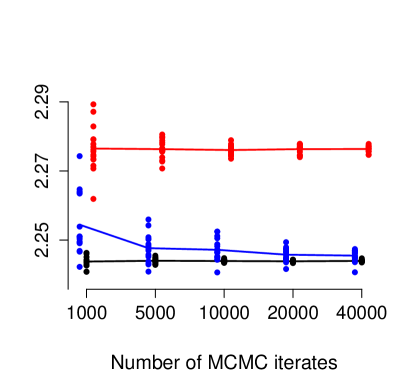
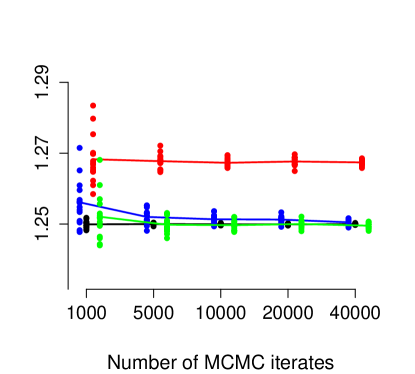
Figure 3: Mean score in the data example against sample size. The dots represent 16 parallel MCMC chains, and the lines connect averages across chains.

6 Discussion

We have investigated how to make and evaluate probabilistic forecasts based on MCMC output. The formal notion of consistency allows us to assess the appropriateness of approximation methods within the framework of proper scoring rules. Despite their popularity in the literature, Gaussian approximations generally fail to be consistent. Conditions for consistency depend on the scoring rule of interest, and we have demonstrated that the mixture-of-parameters and empirical CDF-based approximations are consistent relative to the CRPS under minimal conditions. Proofs of consistency relative to the logarithmic score generally rely on stringent assumptions.

In view of these theoretical considerations as well as the practical perspective taken in our simulation and data examples, we generally recommend the use of the mixture-of-parameters estimator, which provides an efficient approximation method and outperforms all alternatives. This can be explained by the fact that it efficiently exploits the parametric structure of the Bayesian model. The empirical CDF-based approximation provides a good alternative if the conditional distributions fail to be available in closed form, or if for some reason the draws are to be made directly from the posterior predictive distribution, as opposed to using parameter draws. The empirical CDF-based approximation is available under the CRPS and DSS but not under the logarithmic score, where a density is required. Under the logarithmic score, the case for the mixture-of-parameters estimator is thus particularly strong. In particular, the score’s sensitivity to the tails of the distribution renders kernel density estimators unattractive from both theoretical and applied perspectives.

Our recommendations have been implemented in the scoringRules package for R (R Core Team, 2019); see Jordan et al. (2019) for details. The functions and default choices aim to provide readily applicable and efficient approximations. The mixture-of-parameters estimator depends on the specific structure of the Bayesian model and can therefore not be covered in full generality. However, the implemented analytical solutions of the CRPS and logarithmic score allow for straightforward and efficient computation. The scoringRules package further contains functions and data for replicating the simulation and case study, with details provided at https://github.com/FK83/scoringRules/blob/master/KLTG2020_replication.pdf.

Ferro (2014) studies the notion of a fair scoring rule in the context of ensemble weather forecasts. A scoring rule is called fair if the expected score is optimal for samples with members that behave as though they and the verifying observation were sampled from the same distribution. While certainly relevant in the context of meteorological forecast ensembles, where the sample size $m$ is typically between 10 and 50, these considerations seem less helpful in the context of MCMC output, where $m$ is on the order of thousands and can be increased at low cost. Furthermore, the proposed small sample adjustments and the characterization of fair scores hold for independent samples only, an assumption that is thoroughly violated in the case of MCMC.

We are interested in evaluating probabilistic forecasts produced via MCMC, so that the predictive performance of a model during an out-of-sample, test or evaluation period can be used to estimate its forecast performance on future occasions. In contrast, information criteria suggest a different route towards estimating forecast performance (Spiegelhalter et al., 2002; Watanabe, 2010; Hooten and Hobbs, 2015). They consider a method’s in-sample performance, and account for model complexity via penalty terms. Preferred ways of doing so have been the issue of methodological debate, and a consensus has not been reached; see, e.g., the comments in Gelman et al. (2014b) and Spiegelhalter et al. (2014). This present analysis does not concern in-sample comparisons, and does not address the question of whether these are more or less effective than out-of-sample comparisons. However, our results and observations indicate that out-of-sample comparisons of the type considered here yield robust results across a range of implementation choices.

Necessarily, the scope of this paper is restricted along several dimensions. First, our theoretical results focus on consistency but do not cover rates of convergence. Results on the latter tend to rely on theoretical conditions that are hard to verify empirically, and the plausibility of which is likely to depend on the specifics of the MCMC algorithm. In contrast, many of our consistency results require only minimal conditions that hold across a wide range of sampling algorithms in the interdisciplinary applied literature. Second, we have focused on univariate continuous forecast distributions. The corresponding applied literature is large and features a rich variety of implementation variants (cf. Table 1 of the Online Supplement). Nevertheless, there are other empirically relevant setups, notably simple functionals of a predictive distribution, discrete univariate distributions, and continuous multivariate distributions. We briefly discuss each setup in turn.

Functionals such as quantiles summarize a predictive distribution, thus allowing for simpler interpretation and communication (Raftery, 2016). If the forecast user requires only a specific quantile of the predictive distribution, it seems natural to focus on this quantile for evaluation. Interestingly, the CRPS can be represented as the integral over (twice) the asymmetric piecewise linear scoring function which is commonly used to evaluate quantile forecasts (Gneiting and Ranjan, 2011, Equations 11 to 13). Consequently, the CRPS divergence is the integral over the quantile score divergence. In this sense, results for quantiles are covered by our results in terms of the CRPS. The same argument applies if the functional sought is the exceedance probability at any given threshold value, as an immediate consequence of the standard representation of the CRPS (see Equation 7). In order to illustrate the argument numerically, Section S3 of the Online Supplement applies our simulation design to quantiles at two different levels, yielding results that are qualitatively very similar to our CRPS results for full predictive distributions.

In relevant discrete settings, such as predicting probabilities of a binary or categorical outcome, the estimation problem becomes considerably simpler than for the real-valued case. The more complex case of integer-valued count data can be handled using methods similar to the ones we discuss. Instead of probability density functions, the count data case involves probability mass functions to which both the logarithmic score and the CRPS transfer naturally (Czado et al., 2009). Furthermore, all of the approximation methods we discuss can be used in the count data case. For example, the mixture-of-parameters estimator can be used in concert with a Poisson or Negative Binomial specification. Similarly, Shirota and Gelfand (2017, Section 4) consider eq. (10) in a count data context, and kernel-type smoothing methods have been proposed for count data as well (Rajagopalan and Lall, 1995).

The multivariate case features novel challenges. Perhaps most fundamentally, a consensus on practically appropriate choices of the scoring rule is yet to be reached (Gneiting et al., 2008; Scheuerer and Hamill, 2015). Held et al. (2017, Section 4.2) and White et al. (2019, Section 3.3) propose the use of the empirical CDF approximation in concert with the multivariate energy score. In this setting, analogues of our Theorem 3 hold, assuring consistency under weak conditions. For kernel density estimators the ‘curse of dimensionality’ applies, and for the mixture-of-parameters estimator we expect numerical challenges when evaluating, say, a log predictive density in a high-dimensional space. Clearly, there is considerable scope and opportunity for future research in these directions.

Appendix A Computing the CRPS for mixtures of Gaussians

Here we discuss the computation of the CRPS in (7) when the predictive distribution is an equally weighted mixture of normal distributions, say $F=\hat{F}_{m}^{\rm MP}$, where $F_{c}(\cdot\hskip 0.56905pt|\hskip 0.85358pt\theta_{i})$ is Gaussian with mean $\mu_{i}$ and variance $\sigma_{i}^{2}$. Grimit et al. (2006) note that in this case (8) can be written as

$$\text{CRPS}\left(\hat{F}_{m}^{\rm MP},y\right) = \frac{1}{m}\sum_{i=1}^{m}A(y-\mu_{m},\sigma^{2}_{m})-\frac{1}{2m^{2}}\sum_{i=1}^{m}\sum_{j=1}^{m}A(\mu_{i}-\mu_{j},\sigma_{i}^{2}+\sigma_{j}^{2}),$$

where $A(\mu,\sigma^{2})=2\sigma\phi(\frac{\mu}{\sigma})+\mu(2\Phi(\frac{\mu}{\sigma})-1)$, with $\phi$ and $\Phi$ denoting the standard normal density and CDF, respectively. The scoringRules software package (Jordan et al., 2019) contains R/C++ code for the evaluation of (LABEL:eq:Grimit), which requires $\mathcal{O}(m^{2})$ operations.

A potentially much faster, but not exact, alternative is to evaluate the integral in (7) numerically. Here we provide some evidence on the viability of this strategy, which we implement via the R function integrate, with arguments rel.tol and abs.tol of integrate set to $10^{-6}$. As a first experiment, we use numerical integration to re-compute the CRPS scores of the mixture-of-parameters estimator in our data example for the first quarter of 2011. Figure 4 summarizes the results for 16 parallel chains. The left panel shows that the approximate scores are visually identical to the exact ones across all sample sizes and chains. Indeed, the maximal absolute error incurred by numerical integration is $8.0\times 10^{-8}$. The approximation errors are dwarfed by the natural variation of the scores across MCMC chains. The right panel compares the computation time for exact evaluation vs. numerical integration. The latter is much faster, especially for large samples. For a sample of size 40,000 numerical integration requires less than 1.5 seconds, whereas exact evaluation requires about two minutes on an Intel i7 processor.

CRPS	Computation time
	(in seconds)

Figure 4: CRPS scores for the first quarter of 2011 in the data example, for 16 parallel chains and various MCMC sample sizes. Left: The segments connect the CRPS value obtained using numerical integration (left node) to the score obtained using the exact formula (right node). Right: Computation times in seconds, for numerical integration (dots; solid line) and exact formula (crosses; dashed line).

To obtain broad-based evidence, we next compare exact evaluation vs. numerical integration for all 74 forecast dates, from the second quarter of 1996 to the third quarter of 2014, employing 16 parallel chains for each date. We focus on the two largest MCMC sample sizes, 20 000 and 40 000, and find that across all 2 368 instances (74 dates times 2 sample sizes times 16 chains), the absolute difference of the two CRPS values never exceeds $6.3\times 10^{-7}$. Therefore, we feel that numerical integration allows for the efficient evaluation of the CRPS for mixtures of normal distributions. The differences to the exact values are practically irrelevant and well in line with the error bounds in R’s integrate function.

Appendix B Consistency of mixture-of-parameters approximations

Proof of Theorem 1

In the case of the CRPS, we prove the stronger result that $\int_{\mathbb{R}}|\hat{F}_{m}^{\rm MP}(z)-F_{0}(z)|\,{\rm d}z\to 0$ almost surely as $m\to\infty$. Putting $H(z)=1-F_{0}(z)+F_{0}(-z)$ and $\hat{H}_{m}(z)=1-\hat{F}_{m}^{\rm MP}(z)+\hat{F}_{m}^{\rm MP}(-z)$ for $z\in\mathbb{R}$, we find that, for every fixed $N>0$,

$$\limsup_{m\to\infty}\int_{\mathbb{R}}|\hat{F}_{m}^{\rm MP}(z)-F_{0}(z)|\,{\rm d}z \>\leq\>\limsup_{m\to\infty}\int_{-N}^{N}|\hat{F}_{m}^{\rm MP}(z)-F_{0}(z)|\,{\rm d}z$$

$$\qquad+\,\int_{N}^{\infty}\!H(z)\,{\rm d}z\>+\>\limsup_{m\to\infty}\int_{N}^{\infty}\!\hat{H}_{m}(z)\,{\rm d}z.$$ (20)

The Ergodic Theorem implies that the first term on the right-hand side of (20) tends to zero, and that

$$\int_{N}^{\infty}\!\hat{H}_{m}(z)\,{\rm d}z=\int_{N}^{\infty}\frac{1}{m}\sum_{i=1}^{m}\left(1-F_{c}(z\hskip 0.56905pt|\hskip 0.85358pt\theta_{i})+F_{c}(-z\hskip 0.56905pt|\hskip 0.85358pt\theta_{i})\right)\,{\rm d}z\longrightarrow\int_{N}^{\infty}\!H(z)\,{\rm d}z$$

almost surely as $m\to\infty$. In view of (20) we conclude that

$$\limsup_{m\to\infty}\int_{\mathbb{R}}|\hat{F}_{m}^{\rm MP}(z)-F_{0}(z)|\,{\rm d}z\leq 2\,\int_{N}^{\infty}\!H(z)\,{\rm d}z$$ (21)

almost surely as $m\to\infty$. As the right-hand side of (21) decreases to zero as $N$ grows without bounds, the proof of the claim is complete.

In the case of the DSS, let $K(z)=1-F_{0}(z)-F_{0}(-z)$ and $\hat{K}_{m}(z)=1-\hat{F}_{m}^{\rm MP}(z)-\hat{F}_{m}^{\rm MP}(-z)$ for $z\in\mathbb{R}$. Due to the finiteness of the first moments of $F_{0}$ and $\hat{F}_{m}^{\rm MP}$, $\int_{\mathbb{R}}z\,{\rm d}F_{0}(z)=\int_{0}^{\infty}K(z)\,{\rm d}z$ and $\int_{\mathbb{R}}z\,{\rm d}\hat{F}_{m}^{\rm MP}(z)=\int_{0}^{\infty}\hat{K}_{m}(z)\,{\rm d}z$. For the second moments, we find similarly that $\int_{\mathbb{R}}z^{2}\,{\rm d}F_{0}(z)=2\int_{0}^{\infty}zH(z)\,{\rm d}z$ and $\int_{\mathbb{R}}z^{2}\,{\rm d}\hat{F}_{m}^{\rm MP}(z)=2\int_{0}^{\infty}z\hat{H}_{m}(z)\,{\rm d}z$. Proceeding as before, the Ergodic Theorem implies almost sure convergence of the first and second moments, and thereby consistency relative to the DSS.

Proof of Theorem 2

By Lemma 2.1 in Chapter 4 of Kullback (1959),

$$\sup_{z\in\mathbb{R}}\left|1-\frac{\hat{f}_{m}^{\rm MP}(z)}{f_{0}(z)}\right|\longrightarrow 0$$

almost surely as $m\to\infty$ implies the desired convergence of the Kullback-Leibler divergence. Let $P_{m}$ denote the empirical CDF of the parameter draws $(\theta_{i})_{i=1}^{m}$. Under assumption (B) almost sure strong uniform consistency,

$$\sup_{z\in\Omega}\left|\hat{f}_{m}^{\rm MP}(z)-f_{0}(z)\right|=\sup_{z\in\Omega}\left|\int_{\Theta}f_{c}(z|\theta)\left[{\rm d}P_{m}(\theta)-{\rm d}P_{\rm post}(\theta)\right]\right|\longrightarrow 0$$

almost surely as $m\to\infty$, yields Kullback’s condition. Finally, we establish almost sure strong uniform convergence under assumptions (A) and (B) by applying Theorem 19.4 and Example 19.8 of van der Vaart (2000).

Appendix C Consistency of empirical CDF-based approximations

Proof of Theorem 3

In the case of the CRPS, we proceed in analogy to the proof of Theorem 1 and demonstrate the stronger result that $\int_{\mathbb{R}}|\hat{F}_{m}^{\rm ECDF}(z)-F_{0}(z)|\,{\rm d}z\to 0$ almost surely as $m\to\infty$. Putting $H(z)=1-F_{0}(z)+F_{0}(-z)$ and $\hat{H}_{m}(z)=1-\hat{F}_{m}^{\rm ECDF}(z)+\hat{F}_{m}^{\rm ECDF}(-z)$ for $z\in\mathbb{R}$, we see that, for every fixed $N>0$,

$$\limsup_{m\to\infty}\int_{\mathbb{R}}|\hat{F}_{m}^{\rm ECDF}(z)-F_{0}(z)|\,{\rm d}z \>\leq\>\limsup_{m\to\infty}\int_{-N}^{N}|\hat{F}_{m}^{\rm ECDF}(z)-F_{0}(z)|\,{\rm d}z$$

$$\qquad+\,\int_{N}^{\infty}\!H(z)\,{\rm d}z\>+\>\limsup_{m\to\infty}\int_{N}^{\infty}\!\hat{H}_{m}(z)\,{\rm d}z.$$ (22)

The Generalized Glivenko-Cantelli Theorem (Dehling and Philipp, 2002, Theorem 1.1) implies that the first term on the right-hand side of (22) tends to zero almost surely as $m\to\infty$. If $Z_{0}$ has distribution $F_{0}$, then $\int_{N}^{\infty}\!H(z)\,{\rm d}z=\mathbb{E}(|Z_{0}|-N)_{+}$, where $(W)_{+}=\max(W,0)$ denotes the positive part of $W$. Furthermore, by the Ergodic Theorem

$$\int_{N}^{\infty}\!\hat{H}_{m}(z)\,{\rm d}z=\frac{1}{m}\sum_{i=1}^{m}(|X_{i}|-N)_{+}\longrightarrow\mathbb{E}(|Z_{0}|-N)_{+}$$

almost surely as $m\to\infty$, which along with(22) implies that

$$\limsup_{m\to\infty}\int_{\mathbb{R}}|\hat{F}_{m}^{\rm ECDF}(z)-F_{0}(z)|\,{\rm d}z\leq 2\,\mathbb{E}(|Z_{0}|-N)_{+}$$ (23)

almost surely as $m\to\infty$. As the right-hand side of (23) gets arbitrarily close to zero as $N$ grows without bounds, the proof of the claim is complete.

In the case of the DSS, it suffices to note that the moments of the empirical CDF are the sample moments of $(X_{i})_{i=1}^{m}$, and then to apply the Ergodic Theorem.

Proof of Theorem 4

By the law of total expectation, $\mathbb{E}\hat{F}_{m}^{\rm ECDF}(z)=\mathbb{E}\hat{F}_{m}^{\rm MP}(z)$ as

$$\mathbb{E}\left(\hat{F}_{m}^{\rm ECDF}(z)|\theta_{1},\dots,\theta_{m}\right) =\frac{1}{m}\sum_{i=1}^{m}\mathbb{P}\left(X_{i}\leq z|\theta_{1},\dots,\theta_{m}\right)$$

$$=\frac{1}{m}\sum_{i=1}^{m}\mathbb{P}\left(X_{i}\leq z|\theta_{i}\right)$$

$$=\hat{F}_{m}^{\rm MP}(z).$$

Further, the law of total variance implies

$$\text{Var}\left(\hat{F}_{m}^{\rm ECDF}(z)\right) =\mathbb{E}\left[\text{Var}\left(\hat{F}_{m}^{\rm ECDF}(z)|\theta_{1},\dots,\theta_{m}\right)\right]+\text{Var}\left[\mathbb{E}\left(\hat{F}_{m}^{\rm ECDF}(z)|\theta_{1},\dots,\theta_{m}\right)\right]$$

$$\geq\text{Var}\left(\hat{F}_{m}^{\rm MP}(z)\right)$$

for every $z\in\mathbb{R}$ and $m\in\mathbb{N}$. For a generic estimator $\hat{F}_{m}$ with finite mean,

$$\mathbb{E}\leavevmode\nobreak\ d_{\text{CRPS}}(\hat{F}_{m},F_{0}) = \mathbb{E}\int\left(\hat{F}_{m}(z)-F_{0}(z)\right)^{2}\leavevmode\nobreak\ dz$$

$$= \int{\mathbb{E}\left(\hat{F}_{m}(z)-F_{0}(z)\right)^{2}}\leavevmode\nobreak\ dz$$

$$= \int\text{Var}\leavevmode\nobreak\ \hat{F}_{m}(z)\leavevmode\nobreak\ dz+\int\left(\mathbb{E}\hat{F}_{m}(z)-F_{0}(z)\right)^{2}dz.$$

In this light, the first part of the theorem’s statement implies the second part.

Appendix D Simulation Study on Thinning an MCMC sample

Logarithmic score, Mixture-of-parameters	CRPS, Mixture-of-parameters
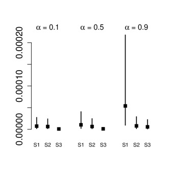
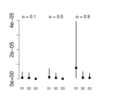
Logarithmic score, Kernel density estimation	CRPS, Empirical CDF

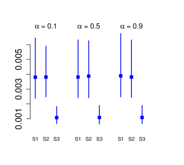
Figure 5: Performance of three sampling strategies: S1: $5\,000$ draws, without thinning; S2: $5\,000$ MCMC draws, retaining every $10$th draw from a sequence of $50\,000$ draws; S3: $50\,000$ draws, without thinning. Bars range from the 10th to the 90th percentile of the score divergences across 1 000 replicates. The squares mark the respective medians.

Using the same simulation setup as in Section 4, we further investigate the effect of thinning the Markov chains. Thinning a chain by a factor of $\tau$ means that only every $\tau$th simulated value is retained, and the rest is discarded. Thinning is often applied routinely with the goal of reducing autocorrelation in the draws. Of the articles listed in Table 1 of the Online Supplement, about one in four explicitly reports thinning of the simulation output, with thinning factors ranging from 2 to 100. Here we compare three sampling approaches:

• $5\,000$ MCMC draws, without thinning

• $5\,000$ MCMC draws, retaining every $10$th draw from a sequence of $50\,000$ draws

• $50\,000$ MCMC draws, without thinning

Note that the samples in S1 and S3 have the same dynamic properties, whereas S2 will typically produce a chain with less autocorrelation. Furthermore, S2 and S3 require the same computing time, which exceeds that of S1 by a factor of ten. Figure 5 summarizes the corresponding simulation results, using parameter values $s=2$ and $n=12$, and varying values of the persistence parameter $\alpha$. We report results for four popular combinations of scoring rules and approximation methods.

As expected, S2 tends to outperform S1: When the sample size is held fixed, less autocorrelation entails more precise estimators. While the difference in performance is modest in most cases, S2 attains large (relative) gains over S1 when the mixture-of-parameters estimator is applied to a very persistent sample with $\alpha=0.9$. This can be explained by the direct effect of the persistence parameter $\alpha$ on the parameter draws $(\theta_{i})_{i=1}^{m}$, whereas the influence is less immediate for the KDE and ECDF approximation methods, which are based on the sequence $(X_{i})_{i=1}^{m}$ obtained in an additional sampling step. Furthermore, S3 outperforms S2 in all cases covered. While the effects of thinning have not been studied in the context of predictive distributions before, this observation is in line with extant reports of the greater precision of unthinned chains (Geyer, 1992; MacEachern and Berliner, 1994; Link and Eaton, 2012). The performance gap between S3 and S2 is modest for the mixture-of-parameters estimator (top row of Figure 5), but very pronounced for the other estimators.

Appendix E Implementation details for the data example

Here we provide additional information on the Markov switching model for the quarterly U.S. GDP growth rate, $Y_{t}$. As described in equation (18) in Section 5, the model is given by $Y_{t}=\nu+\alpha Y_{t-1}+\varepsilon_{t}$, where $\varepsilon_{t}\sim\mathcal{N}(0,\eta^{2}_{s_{t}})$, and $s_{t}\in\{1,2\}$ is a discrete state variable that switches according to a Markov chain.

Table 4: Prior parameters in the Markov switching model.

Symbol in Amisano	$\boldsymbol{\underline{\mu}_{\delta}}$	$\bf{\underline{H}}^{-1}_{\delta}$	$\underline{s}$	$\underline{\nu}$	$\mathbf{R}$
and Giacomini (2007)
Parameter choice	$0_{[2,1]}$	$25\times I_{2}$	0.3	3	$\begin{bmatrix}8&2\\ 2&8\\ \end{bmatrix}$
Relation to our eq. (18)	Prior mean	Prior variance	Prior parameters		Dirichlet prior
	for $(\nu,\alpha)^{\prime}$	for $(\nu,\alpha)^{\prime}$	for $\eta^{2}_{s_{t}}$		state transitions

Our implementation follows Amisano and Giacomini (2007, Section 6.3), in that our prior distributions have the same functional forms but possibly different parameter choices, as summarized in Table 4. However, note that we use prior parameters for the residual variances in both latent states, whereas Amisano and Giacomini (2007) assume the residual variance to be constant across states.

Let $\beta=(\nu,\alpha)^{\prime}$ denote the parameters for the conditional mean equation (18), $\overline{s}_{t}=(s_{1},\ldots,s_{t})^{\prime}$ the sequence of latent states up to time $t$, $h=(\eta_{1}^{-2},\eta_{2}^{-2})^{\prime}$ the inverses of the state-dependent residual variances, and $\mathbf{P}$ the $2\times 2$ transition matrix for the latent states. Our Gibbs sampler can then be sketched as follows:

• Draw $\beta\,|\,h,\overline{s}_{t}$ from a Gaussian posterior. The mean and variance derive from a generalized least squares problem, with observation $t$ receiving weight $\eta^{-2}_{s_{t}}$.

• Draw $h\,|\,\beta,\overline{s}_{t}$ from a Gamma posterior. The Gamma distribution parameters for $\eta_{s}^{-2},s\in\{1,2\},$ are calculated from the observations $t$ for which $s_{t}=s$. If necessary, permute the draws such that $\eta_{1}^{2}>\eta_{2}^{2}$.

• Draw $\overline{s}_{t}\,|\,\beta,h,\mathbf{P}$ using the algorithm described by Greenberg (2013, pp. 194–195).

• Draw $\mathbf{P}\,|\,\overline{s}_{t}$ from a Dirichlet posterior.

Gianni Amisano kindly provides implementation details and Matlab code via his website (https://sites.google.com/site/gianniamisanowebsite/home/teaching/istanbul-2014, last accessed: March 25, 2019). An R implementation of his code is available within the R package scoringRules (Jordan et al., 2019), see https://github.com/FK83/scoringRules/blob/master/KLTG2020_replication.pdf for details.

References

- Amisano and Giacomini (2007) Amisano, G. and Giacomini, R. (2007). Comparing density forecasts via weighted likelihood ratio tests. J. Bus. Econom. Statist., 25, 177–190.
- Barron et al. (1992) Barron, A. R., Györfi, L. and van der Meulen, E. C. (1992). Distribution estimation consistent in total variation and in two types of information divergence. IEEE Trans. Inform. Theory, 38, 1437–1454.
- Bellemare et al. (2017) Bellemare, M. G., Danihelka, I., Dabney, W., Mohamed, S., Lakshminarayanan, B., Hoyer, S. and Munos, R. (2017). The Cramer distance as a solution to biased Wasserstein gradients. Preprint, available at http://arxiv.org/abs/1705.10743.
- Bernardo (1979) Bernardo, J. M. (1979). Expected information as expected utility. Ann. Statist., 7, 686–690.
- Bolin and Wallin (2020) Bolin, D. and Wallin, J. (2020). Multivariate type-G Matérn stochastic partial differential equation random fields. J. R. Stat. Soc. Ser. B. Stat. Methodol., 82, 215–239.
- Brier (1950) Brier, G. W. (1950). Verification of forecasts expressed in terms of probability. Mon. Weather Rev., 78, 1–3.
- Clark (2005) Clark, J. S. (2005). Why environmental scientists are becoming Bayesians. Ecol. Lett., 8, 2–14.
- Clark and McCracken (2013) Clark, T. and McCracken, M. (2013). Advances in forecast evaluation. In Handbook of Economic Forecasting (G. Elliott and A. Timmermann, eds.), vol. 2. Elsevier, 1107–1201.
- Clark and Ravazzolo (2015) Clark, T. E. and Ravazzolo, F. (2015). Macroeconomic forecasting performance under alternative specifications of time-varying volatility. J. Appl. Econometrics, 30, 551–575.
- Cooke (1906) Cooke, W. E. . (1906). Forecasts and verifications in Western Australia. Mon. Weather Rev., 34, 23–24.
- Craiu and Rosenthal (2014) Craiu, R. V. and Rosenthal, J. S. (2014). Bayesian computation via Markov chain Monte Carlo. Annu. Rev. Stat. Appl., 1, 179–201.
- Czado et al. (2009) Czado, C., Gneiting, T. and Held, L. (2009). Predictive model assessment for count data. Biometrics, 65, 1254–1261.
- Dawid (1984) Dawid, A. P. (1984). Present position and potential developments: Some personal views. Statistical theory: The prequential approach. J. R. Stat. Soc. Ser. A. Gen., 147, 278–290.
- Dawid and Sebastiani (1999) Dawid, A. P. and Sebastiani, P. (1999). Coherent dispersion criteria for optimal experimental design. Ann. Statist., 27, 65–81.
- Dehling and Philipp (2002) Dehling, H. and Philipp, W. (2002). Empirical process techniques for dependent data. In Empirical Process Techniques for Dependent Data (H. Dehling, T. Mikosch and M. Sørensen, eds.). Birkhäuser, Boston, 3–113.
- DelSole and Tippett (2014) DelSole, T. and Tippett, M. K. (2014). Comparing forecast skill. Mon. Weather Rev., 142, 4658–4678.
- Diebold et al. (1998) Diebold, F. X., Gunther, T. A. and Tay, A. S. (1998). Evaluating density forecasts with applications to financial risk management. Internat. Econom. Rev., 39, 863–883.
- Diebold and Mariano (1995) Diebold, F. X. and Mariano, R. S. (1995). Comparing predictive accuracy. J. Bus. Econom. Statist., 13, 253–263.
- Feldmann et al. (2015) Feldmann, K., Scheuerer, M. and Thorarinsdottir, T. L. (2015). Spatial postprocessing of ensemble forecasts for temperature using nonhomogeneous gaussian regression. Mon. Weather Rev., 143, 955–971.
- Ferro (2014) Ferro, C. A. T. (2014). Fair scores for ensemble forecasts. Q. J. Royal Meteorol. Soc., 140, 1917–1923.
- Fox and West (2011) Fox, E. B. and West, M. (2011). Autoregressive models for variance matrices: Stationary inverse Wishart processes. Preprint, available at http://arxiv.org/abs/1107.5239.
- Gelfand and Smith (1990) Gelfand, A. E. and Smith, A. F. M. (1990). Sampling-based approaches to calculating marginal densities. J. Amer. Statist. Assoc., 85, 398–409.
- Gelman et al. (2014a) Gelman, A., Carlin, J. B., Stern, H. S., Dunson, D. B., Vehtari, A. and Rubin, D. B. (2014a). Bayesian Data Analysis. 3rd ed. Chapman & Hall/CRC, Boca Raton.
- Gelman et al. (2014b) Gelman, A., Hwang, J. and Vehtari, A. (2014b). Understanding predictive information criteria for Bayesian models. Stat. Comput., 24, 997–1016.
- Gelman et al. (1996) Gelman, A., Meng, X.-L. and Stern, H. (1996). Posterior predictive assessment of model fitness via realized discrepancies. Statist. Sinica, 6, 733–760.
- Genon-Catalot et al. (2000) Genon-Catalot, V., Jeantheau, T. and Larédo, C. (2000). Stochastic volatility models as hidden Markov models and statistical applications. Bernoulli, 6, 1051–1079.
- Geweke (2005) Geweke, J. (2005). Contemporary Bayesian Econometrics and Statistics. John Wiley & Sons, Hoboken.
- Geyer (1992) Geyer, C. J. (1992). Practical Markov chain Monte Carlo. Statist. Sci., 7, 473–483.
- Giacomini and White (2006) Giacomini, R. and White, H. (2006). Tests of conditional predictive ability. Econometrica, 74, 1545–1578.
- Gibbs and Su (2002) Gibbs, A. L. and Su, F. E. (2002). On choosing and bounding probability metrics. Int. Stat. Rev., 70, 419–435.
- Gilks et al. (1996) Gilks, W. R., Richardson, S. and Spiegelhalter, D. J. (eds.) (1996). Markov Chain Monte Carlo in Practice. Chapman & Hall/CRC, Boca Raton.
- Gneiting (1997) Gneiting, T. (1997). Normal scale mixtures and dual probability densities. J. Stat. Comput. Simul., 59, 375–384.
- Gneiting and Raftery (2007) Gneiting, T. and Raftery, A. E. (2007). Strictly proper scoring rules, prediction, and estimation. J. Amer. Statist. Assoc., 102, 359–378.
- Gneiting and Ranjan (2011) Gneiting, T. and Ranjan, R. (2011). Comparing density forecasts using threshold- and quantile-weighted scoring rules. J. Bus. Econom. Statist., 29, 411–422.
- Gneiting et al. (2008) Gneiting, T., Stanberry, L. I., Grimit, E. P., Held, L. and Johnson, N. A. (2008). Assessing probabilistic forecasts of multivariate quantities, with an application to ensemble predictions of surface winds (with discussion and rejoinder). Test, 17, 211–264.
- Good (1952) Good, I. J. (1952). Rational decisions. J. R. Stat. Soc. Ser. B. Stat. Methodol., 14, 107–114.
- Greenberg (2013) Greenberg, E. (2013). Introduction to Bayesian Econometrics. 2nd ed. Cambridge University Press, New York.
- Grimit et al. (2006) Grimit, E. P., Gneiting, T., Berrocal, V. J. and Johnson, N. A. (2006). The continuous ranked probability score for circular variables and its application to mesoscale forecast ensemble verification. Q. J. Royal Meteorol. Soc., 132, 2925–2942.
- Györfi et al. (1989) Györfi, L., Härdle, W., Sarda, P. and Vieu, P. (1989). Nonparametric Curve Estimation from Time Series. Springer, Berlin.
- Hall (1987) Hall, P. (1987). On Kullback-Leibler loss and density estimation. Ann. Statist., 15, 1491–1519.
- Hall et al. (1995) Hall, P., Lahiri, S. N. and Truong, Y. K. (1995). On bandwidth choice for density estimation with dependent data. Ann. Statist., 23, 2241–2263.
- Hall and Presnell (1999) Hall, P. and Presnell, B. (1999). Density estimation under constraints. J. Comput. Graph. Statist., 8, 259–277.
- Hamilton (1989) Hamilton, J. D. (1989). A new approach to the economic analysis of nonstationary time series and the business cycle. Econometrica, 57, 357–384.
- Hansen (2008) Hansen, B. E. (2008). Uniform convergence rates for kernel estimation with dependent data. Econom. Theory, 24, 726–748.
- Harris (1989) Harris, I. R. (1989). Predictive fit for natural exponential families. Biometrika, 76, 675–684.
- Held et al. (2017) Held, L., Meyer, S. and Bracher, J. (2017). Probabilistic forecasting in infectious disease epidemiology: The 13th Armitage lecture. Stat. Med., 36, 3443–3460.
- Held et al. (2010) Held, L., Schrödle, B. and Rue, H. (2010). Posterior and cross-validatory predictive checks: A comparison of MCMC and INLA. In Statistical Modelling and Regression Structures: Festschrift in Honour of Ludwig Fahrmeir (T. Kneib and G. Tutz, eds.). Physica-Verlag HD, Heidelberg, 91–110.
- Hooten and Hobbs (2015) Hooten, M. B. and Hobbs, N. T. (2015). A guide to Bayesian model selection for ecologists. Ecol. Monogr., 85, 3–28.
- Huber and Ronchetti (2009) Huber, P. J. and Ronchetti, E. M. (2009). Robust Statistics. 2nd ed. Wiley, Hoboken, New Jersey.
- Jones (1991) Jones, M. C. (1991). On correcting for variance inflation in kernel density estimation. Comput. Stat. Data Anal., 11, 3–15.
- Jordan (2016) Jordan, A. (2016). Facets of forecast evaluation. Ph.D. thesis, Karlsruhe Institute of Technology, available at https://publikationen.bibliothek.kit.edu/1000063629.
- Jordan et al. (2019) Jordan, A., Krüger, F. and Lerch, S. (2019). Evaluating probabilistic forecasts with scoringRules. J. Stat. Softw., 90, 1–37.
- Kass and Raftery (1995) Kass, R. E. and Raftery, A. E. (1995). Bayes factors. J. Amer. Statist. Assoc., 90, 773–795.
- Kim et al. (2016) Kim, H. J., MacEachern, S. N. and Jung, Y. (2016). Bandwidth selection for kernel density estimation with a Markov chain Monte Carlo sample. Preprint, available at http://arxiv.org/abs/1607.08274.
- Krüger et al. (2017) Krüger, F., Clark, T. E. and Ravazzolo, F. (2017). Using entropic tilting to combine BVAR forecasts with external nowcasts. J. Bus. Econom. Statist., 35, 470–485.
- Kullback (1959) Kullback, S. (1959). Information Theory and Statistics. John Wiley & Sons.
- Liebscher (1996) Liebscher, E. (1996). Strong convergence of sums of -mixing random variables with applications to density estimation. Stochastic Process. Appl., 65, 69–80.
- Link and Eaton (2012) Link, W. A. and Eaton, M. J. (2012). On thinning of chains in MCMC. Methods Ecol. Evol., 3, 112–115.
- Little (2006) Little, R. J. (2006). Calibrated Bayes: A Bayes/frequentist roadmap. Amer. Statist., 60, 213–223.
- MacEachern and Berliner (1994) MacEachern, S. N. and Berliner, L. M. (1994). Subsampling the Gibbs sampler. Amer. Statist., 48, 188–190.
- Matheson and Winkler (1976) Matheson, J. E. and Winkler, R. L. (1976). Scoring rules for continuous probability distributions. Manag. Sci., 22, 1087–1096.
- Panaretos and Zemel (2019) Panaretos, V. M. and Zemel, Y. (2019). Statistical aspects of Wasserstein distances. Annu. Rev. Stat. Appl., 6, 405–431.
- R Core Team (2019) R Core Team (2019). R: A Language and Environment for Statistical Computing. R Foundation for Statistical Computing, Vienna, Austria. URL https://www.R-project.org/.
- Raftery (2016) Raftery, A. E. (2016). Use and communication of probabilistic forecasts. Stat. Anal. Data. Min., 9, 397–410.
- Rajagopalan and Lall (1995) Rajagopalan, B. and Lall, U. (1995). A kernel estimator for discrete distributions. J. Nonparametr. Stat., 4, 409–426.
- Rosenblatt (1956) Rosenblatt, M. (1956). Remarks on some nonparametric estimates of a density function. Ann. Math. Stat., 27, 832–837.
- Rosenthal (1995) Rosenthal, J. S. (1995). Minorization conditions and convergence rates for Markov chain Monte Carlo. J. Amer. Statist. Assoc., 90, 558–566.
- Roussas (1988) Roussas, G. G. (1988). Nonparametric estimation in mixing sequences of random variables. J. Statist. Plann. Inference, 18, 135–149.
- Rubin (1984) Rubin, D. B. (1984). Bayesianly justifiable and relevant frequency calculations for the applied statistician. Ann. Statist., 12, 1151–1172.
- Scheuerer and Hamill (2015) Scheuerer, M. and Hamill, T. M. (2015). Variogram-based proper scoring rules for probabilistic forecasts of multivariate quantities. Mon. Weather Rev., 143, 1321–1334.
- Sheather and Jones (1991) Sheather, S. J. and Jones, M. C. (1991). A reliable data-based bandwidth selection method for kernel density estimation. J. R. Stat. Soc. Ser. B. Stat. Methodol., 53, 683–690.
- Shirota and Gelfand (2017) Shirota, S. and Gelfand, A. E. (2017). Space and circular time log Gaussian Cox processes with application to crime event data. The Annals of Applied Statistics, 11, 481–503.
- Shuford et al. (1966) Shuford, E. H., Albert, A. and Massengill, H. E. (1966). Admissible probability measurement procedures. Psychometrika, 31, 125–145.
- Silverman (1986) Silverman, B. W. (1986). Density Estimation for Statistics and Data Analysis. Chapman and Hall, London.
- Sköld and Roberts (2003) Sköld, M. and Roberts, G. O. (2003). Density estimation for the Metropolis-Hastings algorithm. Scand. J. Stat., 30, 699–718.
- Spiegelhalter et al. (2002) Spiegelhalter, D. J., Best, N. G., Carlin, B. P. and van der Linde, A. (2002). Bayesian measures of model complexity and fit (with discussion and rejoinder). J. R. Stat. Soc. Ser. B. Stat. Methodol., 64, 583–639.
- Spiegelhalter et al. (2014) Spiegelhalter, D. J., Best, N. G., Carlin, B. P. and van der Linde, A. (2014). The deviance information criterion: 12 years on. J. R. Stat. Soc. Ser. B. Stat. Methodol., 76, 485–493.
- Taillardat et al. (2016) Taillardat, M., Mestre, O., Zamo, M. and Naveau, P. (2016). Calibrated ensemble forecasts using quantile regression forests and ensemble model output statistics. Mon. Weather Rev., 144, 2375–2393.
- Tanner and Wong (1987) Tanner, M. A. and Wong, W. H. (1987). The calculation of posterior distributions by data augmentation. J. Amer. Statist. Assoc., 82, 528–540.
- Thorarinsdottir et al. (2013) Thorarinsdottir, T. L., Gneiting, T. and Gissibl, N. (2013). Using proper divergence functions to evaluate climate models. SIAM/ASA J. Uncertain. Quantif., 1, 522–534.
- Tierney (1994) Tierney, L. (1994). Markov chains for exploring posterior distributions. Ann. Statist., 22, 1701–1728.
- van der Vaart (2000) van der Vaart, A. W. (2000). Asymptotic Statistics. Cambridge University Press, Cambridge.
- Villani (2008) Villani, C. (2008). Optimal Transport. Grundlehren der mathematischen Wissenschaften, 338, Springer, Berlin, Heidelberg.
- Waggoner and Zha (1999) Waggoner, D. F. and Zha, T. (1999). Conditional forecasts in dynamic multivariate models. Rev. Econ. Stat., 81, 639–651.
- Warne et al. (2016) Warne, A., Coenen, G. and Christoffel, K. (2016). Marginalized predictive likelihood comparisons of linear Gaussian state-space models with applications to DSGE, DSGE-VAR and VAR models. J. Appl. Econometrics, 32, 103–119.
- Wasserman (2006) Wasserman, L. (2006). All of Nonparametric Statistics. Springer, New York.
- Watanabe (2010) Watanabe, S. (2010). Asymptotic equivalence of Bayes cross validation and widely applicable information criterion in singular learning theory. J. Mach. Learn. Res., 11, 3571–3594.
- White et al. (2019) White, P. A., Gelfand, A. E., Rodrigues, E. R. and Tzintzun, G. (2019). Pollution state modelling for Mexico City. J. R. Stat. Soc. Ser. A. Stat. Soc., 182, 1039–1060.
- Yu (1993) Yu, B. (1993). Density estimation in the norm for dependent data with applications to the Gibbs sampler. Ann. Statist., 21, 711–735.
Acknowledgements
The work of Tilmann Gneiting and Fabian Krüger was funded by the European Union Seventh Framework Programme under grant agreement 290976. Sebastian Lerch and Thordis L. Thorarinsdottir acknowledge support by the Volkswagen Foundation through the program “Mesoscale Weather Extremes — Theory, Spatial Modelling and Prediction (WEX-MOP)”. Lerch further acknowledges support by Deutsche Forschungsgemeinschaft (DFG) through RTG 1953 “Statistical Modeling of Complex Systems and Processes” and SFB/TRR 165 “Waves to Weather”. Gneiting, Krüger and Lerch thank the Klaus Tschira Foundation for infrastructural support at the Heidelberg Institute for Theoretical Studies (HITS). Helpful comments by Werner Ehm, Sylvia Frühwirth-Schnatter, Alexander Jordan, as well as seminar and conference participants at HITS, KIT, University of Bern, University of Bonn, University of Oslo, the Extremes 2014 symposium (Hannover), CFE (Pisa, 2014), GPSD (Bochum, 2016), ISBA (Sardinia, 2016), and Deutsche Bundesbank (Workshop on Forecasting, 2017) are gratefully acknowledged. We thank Gianni Amisano for sharing his program code for Bayesian Markov switching models. Furthermore, we thank an anonymous referee of a previous version of the manuscript for pointing us to the Rao-Blackwellization arguments employed in Theorem 4, and another anonymous referee for thoughtful comments on the paper.