Study on the Idle Mode Capability with
LoS and NLoS Transmissions

Abstract

In this paper, we study the impact of the base station (BS) idle mode capability (IMC) on the network performance in dense small cell networks (SCNs). Different from existing works, we consider a sophisticated path loss model incorporating both line-of-sight (LoS) and non-line-of-sight (NLoS) transmissions. Analytical results are obtained for the coverage probability and the area spectral efficiency (ASE) performance for SCNs with IMCs at the BSs. The upper bound, the lower bound and the approximate expression of the activated BS density are also derived. The performance impact of the IMC is shown to be significant. As the BS density surpasses the UE density, thus creating a surplus of BSs, the coverage probability will continuously increase toward one. For the practical regime of the BS density, the results derived from our analysis are distinctively different from existing results, and thus shed new light on the deployment and the operation of future dense SCNs.

I Introduction

Dense small cell networks (SCNs) have attracted much attention as one of the most promising approaches to rapidly increase network capacity and meet the ever-increasing capacity demands [1]. Indeed, the orthogonal deployment of dense SCNs within the existing macrocell networks [2] has been selected as the workhorse for capacity enhancement in the 3rd Generation Partnership Project (3GPP) 4th-generation (4G) and the 5th-generation (5G) networks. This is due to its large spectrum reuse and its easy management [3]; the latter one arising from its low interaction with the macrocell tier, e.g., no inter-tier interference. In this paper, the focus is on the analysis of these dense SCNs with an orthogonal deployment in the existing macrocell networks.

Before 2015, the common understanding on dense SCNs was that the density of base stations (BSs) would not affect the per-BS coverage probability performance in interference-limited fully-loaded wireless networks [4], where the coverage probability is defined as the probability that the signal-to-interference-plus-noise ratio (SINR) of a typical user equipment (UE) is above a SINR threshold $\gamma$. Consequently, the area spectral efficiency (ASE) performance in $\textrm{bps/Hz/km}^{2}$ would scale linearly with the network densification [4]. The intuition of such conclusion is that the increase in the interference power caused by a denser network would be exactly compensated by the increase in the signal power due to the reduced distance between transmitters and receivers. Fig. 1 shows this theoretical coverage probability behavior predicted in [4]. However, it is important to note that such conclusion was obtained with considerable simplifications on the UE deployment and propagation environment, e.g., all BSs were activated considering an infinite UE density. Moreover, a single-slope path loss model was used, which should be placed under scrutiny when evaluating practical dense SCNs, since they are fundamentally different from sparse ones [3].

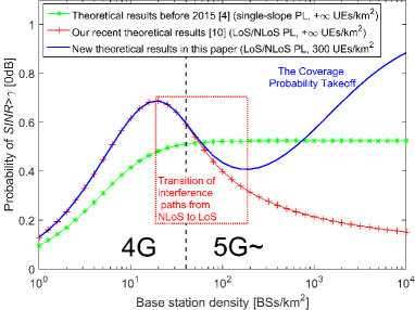
Fig. 1: Theoretical comparison of the coverage probability performance when the SINR threshold $\gamma=0$ dB. Note that all the results are obtained using practical 3GPP channel models [5, 6], which will be introduced in details later. Moreover, the BS density regions for the 4G and the 5G networks have been illustrated in the figure, considering that the typical BS density of the 4G SCNs is in the order of tens of $\textrm{BSs/km}^{2}$ [2, 3].

A few noteworthy studies have been carried out in the last year to revisit the network performance analysis for dense SCNs under more practical propagation assumptions. In [7], the authors considered a multi-slope piece-wise path loss function, while in [8], the authors investigated line-of-sight (LoS) and non-line-of-sight (NLoS) transmission as a probabilistic event for a millimeter wave communication scenario. In our very recent work [9, 10], we took a step further and generalized these works by considering both piece-wise path loss functions and probabilistic LoS and NLoS transmissions. Our new finding was not only quantitatively but also qualitatively different from the results in [4, 7, 8]. In more detail, our analysis demonstrated that when the BS density is larger than a threshold $\lambda^{*}$, the coverage probability performance will decrease as the SCN becomes denser, which in turn may make the ASE suffer from a slow growth or even a decrease on the journey from 4G to 5G. The intuition behind this result is that the interference power increases faster than the signal power due to the transition of a large number of interference paths from NLoS to LoS with the network densification. Our analysis also demonstrated that the decrease of the coverage probability gradually slows down as the SCN becomes ultra-dense. This is because both the interference power and the signal power are LoS dominated and thus statistically stable. Fig. 1 shows this new theoretical coverage probability result, where $\lambda^{*}$ is around 20 $\textrm{BSs/km}^{2}$.

Fortunately, the UE density is finite in practice, and thus a large number of SCN BSs could be switched off in dense SCNs, if there is no active UE within their coverage areas, which mitigates unnecessary inter-cell interference and reduces energy consumption [11, 12, 13]. In more detail, by dynamically turning off idle BSs, the interference suffered by UEs from always-on channels, e.g., synchronization and broadcast channels, and data channels can be reduced, thus improving UEs’ coverage probability. Besides, the energy efficiency of the SCNs can be significantly enhanced because (i) BSs without any active UE can be put into a zero/low-power idle mode until a UE becomes active in its coverage area, and (ii) activated BSs usually enjoy high-SINR links, i.e., energy-efficient links, with their associated UEs thanks to the BS selection from a surplus of BSs. Such capability of idle mode at the BSs is referred to as the idle mode capability (IMC) hereafter.

In this paper, we investigate for the first time the impact of the IMC on the coverage probability performance. Our new theoretical results with a UE density of $300\thinspace\textrm{UEs/km}^{2}$, a typical UE density in 5G [3], are compared with the existing results [4, 10] in Fig. 1. The performance impact of the IMC is shown to be significant: as the BS density surpasses the UE density, thus creating a surplus of BSs, the coverage probability will continuously increase toward one, addressing the issue caused by the NLoS to LoS transition of interfering paths. Such performance behavior is referred to as the Coverage Probability Takeoff hereafter. The intuition behind the Coverage Probability Takeoff is that the interference power will remain constant with the network densification due to the IMC at the BSs, while the signal power will continuously grow due to the BS selection and the shorter BS-to-UE distance, thus permitting stronger serving BS links.

The main contributions of this paper are as follows:

• Analytical results are obtained for the coverage probability and the ASE performance for SCNs with IMC at the BSs using a general path loss model incorporating both LoS and NLoS transmissions. Note that the existing works on the IMC only treat single-slope path loss models where UEs are always associated with the nearest BS [11, 13], while our work considers more practical path loss models with LoS and NLoS transmissions where UEs may connect to a farther BS with a LoS path.

• The upper bound, the lower bound and the approximate expression of the activated BS density are derived for the SCNs with IMCs considering practical path loss models with LoS and NLoS transmissions.

II System Model

We consider a downlink (DL) cellular network with BSs deployed on a plane according to a homogeneous Poisson point process (HPPP) $\Phi$ of intensity $\lambda$ $\textrm{BSs/km}^{2}$. Active UEs are Poisson distributed in the considered network with an intensity of $\rho$ $\textrm{UEs/km}^{2}$. Here, we only consider active UEs in the network because non-active UEs do not trigger data transmission, and thus they are ignored in our analysis.

In our previous works [9, 10] and other related works [7, 8], $\rho$ was assumed to be sufficiently larger than $\lambda$ so that each BS has at least one associated UE in its coverage. In this work, we impose no such constraint on $\rho$, and hence a BS with the IMC will be switched off if there is no UE connected to it, which reduces interference to neighboring UEs as well as energy consumption. Since UEs are randomly and uniformly distributed in the network, we adopt a common assumption that the activated BSs also follow an HPPP distribution $\tilde{\Phi}$ [11], the intensity of which is denoted by $\tilde{\lambda}$ $\textrm{BSs/km}^{2}$. Note that $0\leq\tilde{\lambda}\leq\lambda$ and a larger $\rho$ requires more BSs with a larger $\tilde{\lambda}$ to serve the active UEs.

Following [9, 10], we adopt a very general and practical path loss model, in which the path loss $\zeta\left(r\right)$ associated with distance $r$ is segmented into $N$ pieces written as

$$\zeta\left(r\right)=\begin{cases}\zeta_{1}\left(r\right),&\textrm{when }0\leq r\leq d_{1}\\ \zeta_{2}\left(r\right),&\textrm{when }d_{1}<r\leq d_{2}\\ \vdots&\vdots\\ \zeta_{N}\left(r\right),&\textrm{when }r>d_{N-1}\end{cases},$$ (1)

where each piece $\zeta_{n}\left(r\right),n\in\left\{1,2,\ldots,N\right\}$ is modeled as

$$\zeta_{n}\left(r\right)=\begin{cases}\begin{array}[]{l}\zeta_{n}^{\textrm{L}}\left(r\right)=A_{n}^{{\rm{L}}}r^{-\alpha_{n}^{{\rm{L}}}},\\ \zeta_{n}^{\textrm{NL}}\left(r\right)=A_{n}^{{\rm{NL}}}r^{-\alpha_{n}^{{\rm{NL}}}},\end{array}&\begin{array}[]{l}\textrm{LoS:}\leavevmode\nobreak\ \textrm{Pr}_{n}^{\textrm{L}}\left(r\right)\\ \textrm{NLoS:}\leavevmode\nobreak\ 1-\textrm{Pr}_{n}^{\textrm{L}}\left(r\right)\end{array},\end{cases}$$ (2)

where $\zeta_{n}^{\textrm{L}}\left(r\right)$ and $\zeta_{n}^{\textrm{NL}}\left(r\right),n\in\left\{1,2,\ldots,N\right\}$ are the $n$-th piece path loss functions for the LoS transmission and the NLoS transmission, respectively, $A_{n}^{{\rm{L}}}$ and $A_{n}^{{\rm{NL}}}$ are the path losses at a reference distance $r=1$ for the LoS and the NLoS cases, respectively, and $\alpha_{n}^{{\rm{L}}}$ and $\alpha_{n}^{{\rm{NL}}}$ are the path loss exponents for the LoS and the NLoS cases, respectively. In practice, $A_{n}^{{\rm{L}}}$, $A_{n}^{{\rm{NL}}}$, $\alpha_{n}^{{\rm{L}}}$ and $\alpha_{n}^{{\rm{NL}}}$ are constants obtainable from field tests [5, 6]. Moreover, $\textrm{Pr}_{n}^{\textrm{L}}\left(r\right)$ is the $n$-th piece LoS probability function that a transmitter and a receiver separated by a distance $r$ have a LoS path, which is assumed to be a monotonically decreasing function with regard to $r$.

For convenience, $\left\{\zeta_{n}^{\textrm{L}}\left(r\right)\right\}$ and $\left\{\zeta_{n}^{\textrm{NL}}\left(r\right)\right\}$ are further stacked into piece-wise functions written as

$$\zeta^{Path}\left(r\right)=\begin{cases}\zeta_{1}^{Path}\left(r\right),&\textrm{when }0\leq r\leq d_{1}\\ \zeta_{2}^{Path}\left(r\right),&\textrm{when }d_{1}<r\leq d_{2}\\ \vdots&\vdots\\ \zeta_{N}^{Path}\left(r\right),&\textrm{when }r>d_{N-1}\end{cases},$$ (3)

where the string variable $Path$ takes the value of “L” and “NL” for the LoS and the NLoS cases, respectively.

Besides, $\left\{\textrm{Pr}_{n}^{\textrm{L}}\left(r\right)\right\}$ is stacked into a piece-wise function as

$$\textrm{Pr}^{\textrm{L}}\left(r\right)=\begin{cases}\textrm{Pr}_{1}^{\textrm{L}}\left(r\right),&\textrm{when }0\leq r\leq d_{1}\\ \textrm{Pr}_{2}^{\textrm{L}}\left(r\right),&\textrm{when }d_{1}<r\leq d_{2}\\ \vdots&\vdots\\ \textrm{Pr}_{N}^{\textrm{L}}\left(r\right),&\textrm{when }r>d_{N-1}\end{cases}.$$ (4)

Note that the generality and the practicality of the adopted path loss model (1) have been well established in [10].

In this paper, we also assume a practical user association strategy (UAS), in which each UE should be connected to the BS with the smallest path loss (i.e., with the largest $\zeta\left(r\right)$) to the UE [8, 10]. Note that in our previous work [9] and some existing works [4, 7], it was assumed that each UE should be associated with the BS at the closest proximity. Such assumption is not appropriate for the considered path loss model in (1), because in practice it is possible for a UE to connect to a BS that is not the nearest one but with a LoS path, which is stronger that the NLoS path of the nearest one. Moreover, we assume that each BS/UE is equipped with an isotropic antenna, and that the multi-path fading between a BS and a UE is modeled as independently identical distributed (i.i.d.) Rayleigh fading [7, 8, 9, 10].

III Main Results

Using the HPPP theory, we study the performance of the SCNs by considering the performance of a typical UE located at the origin $o$.

III-A The Coverage Probability

First, we investigate the coverage probability that the typical UE’s SINR is above a designated threshold $\gamma$:

$$p^{\textrm{cov}}\left(\lambda,\gamma\right)=\textrm{Pr}\left[\mathrm{SINR}>\gamma\right],$$ (5)

where the SINR is computed by

$$\mathrm{SINR}=\frac{P\zeta\left(r\right)h}{I_{\textrm{agg}}+P_{{\rm{N}}}},$$ (6)

where $h$ is the channel gain, which is modeled as an exponential random variable (RV) with the mean of one due to our consideration of Rayleigh fading mentioned above, $P$ and $P_{{\rm{N}}}$ are the BS transmission power and the additive white Gaussian noise (AWGN) power at each UE, respectively, and $I_{\textrm{agg}}$ is the cumulative interference given by

$$I_{\textrm{agg}}=\sum_{i:\,b_{i}\in\tilde{\Phi}\setminus b_{o}}P\beta_{i}g_{i},$$ (7)

where $b_{o}$ is the BS serving the typical UE located at distance $r$ from the typical UE, and $b_{i}$, $\beta_{i}$ and $g_{i}$ are the $i$-th interfering BS, the path loss associated with $b_{i}$ and the multi-path fading channel gain associated with $b_{i}$, respectively. Note that in our previous works [9, 10], all BSs were assumed to be powered on, and thus $\Phi$ was used in the expression of $I_{\textrm{agg}}$. Here, in (7), only the activated BSs in $\tilde{\Phi}\setminus b_{o}$ inject effective interference into the network, and thus the other BSs in idle modes are not taken into account in the analysis of $I_{\textrm{agg}}$.

Based on the path loss model in (1) and the considered UAS, we present our result of $p^{\textrm{cov}}\left(\lambda,\gamma\right)$ in Theorem 1 shown on the top of the next page. It is important to note that:

Theorem 1.

Considering the path loss model in (1) and the presented UAS, the probability of coverage $p^{{\rm{cov}}}\left(\lambda,\gamma\right)$ can be derived as

$$p^{{\rm{cov}}}\left(\lambda,\gamma\right)=\sum_{n=1}^{N}\left(T_{n}^{{\rm{L}}}+T_{n}^{{\rm{NL}}}\right),$$ (8)

where $T_{n}^{{\rm{L}}}=\int_{d_{n-1}}^{d_{n}}{\rm{Pr}}\left[\frac{P\zeta_{n}^{{\rm{L}}}\left(r\right)h}{I_{{\rm{agg}}}+P_{{\rm{N}}}}>\gamma\right]f_{R,n}^{{\rm{L}}}\left(r\right)dr$, $T_{n}^{{\rm{NL}}}=\int_{d_{n-1}}^{d_{n}}{\rm{Pr}}\left[\frac{P\zeta_{n}^{{\rm{NL}}}\left(r\right)h}{I_{{\rm{agg}}}+P_{{\rm{N}}}}>\gamma\right]f_{R,n}^{{\rm{NL}}}\left(r\right)dr$, and $d_{0}$ and $d_{N}$ are defined as $0$ and $+\infty$, respectively. Moreover, $f_{R,n}^{{\rm{L}}}\left(r\right)$ and $f_{R,n}^{{\rm{NL}}}\left(r\right)$ $\left(d_{n-1}<r\leq d_{n}\right)$, are represented by

$$f_{R,n}^{{\rm{L}}}\left(r\right)=\exp\left(-\int_{0}^{r_{1}}\left(1-{\rm{Pr}}^{{\rm{L}}}\left(u\right)\right)2\pi u\lambda du\right)\exp\left(-\int_{0}^{r}{\rm{Pr}}^{{\rm{L}}}\left(u\right)2\pi u\lambda du\right){\rm{Pr}}_{n}^{{\rm{L}}}\left(r\right)2\pi r\lambda,$$ (9)

and

$$f_{R,n}^{{\rm{NL}}}\left(r\right)=\exp\left(-\int_{0}^{r_{2}}{\rm{Pr}}^{{\rm{L}}}\left(u\right)2\pi u\lambda du\right)\exp\left(-\int_{0}^{r}\left(1-{\rm{Pr}}^{{\rm{L}}}\left(u\right)\right)2\pi u\lambda du\right)\left(1-{\rm{Pr}}_{n}^{{\rm{L}}}\left(r\right)\right)2\pi r\lambda,$$ (10)

where $r_{1}$ and $r_{2}$ are given implicitly by the following equations as

$$r_{1}=\underset{r_{1}}{\arg}\left\{\zeta^{{\rm{NL}}}\left(r_{1}\right)=\zeta_{n}^{{\rm{L}}}\left(r\right)\right\},$$ (11)

and

$$r_{2}=\underset{r_{2}}{\arg}\left\{\zeta^{{\rm{L}}}\left(r_{2}\right)=\zeta_{n}^{{\rm{NL}}}\left(r\right)\right\}.$$ (12)

In addition, ${\rm{Pr}}\left[\frac{P\zeta_{n}^{{\rm{L}}}\left(r\right)h}{I_{{\rm{agg}}}+P_{{\rm{N}}}}>\gamma\right]$ and ${\rm{Pr}}\left[\frac{P\zeta_{n}^{{\rm{NL}}}\left(r\right)h}{I_{{\rm{agg}}}+P_{{\rm{N}}}}>\gamma\right]$ are respectively computed by

$${\rm{Pr}}\left[\frac{P\zeta_{n}^{{\rm{L}}}\left(r\right)h}{I_{{\rm{agg}}}+P_{{\rm{N}}}}>\gamma\right]=\exp\left(-\frac{\gamma P_{{\rm{N}}}}{P\zeta_{n}^{{\rm{L}}}\left(r\right)}\right)\mathscr{L}_{I_{{\rm{agg}}}}^{{\rm{L}}}\left(\frac{\gamma}{P\zeta_{n}^{{\rm{L}}}\left(r\right)}\right),$$ (13)

where $\mathscr{L}_{I_{{\rm{agg}}}}^{{\rm{L}}}\left(s\right)$ is the Laplace transform of $I_{{\rm{agg}}}$ for LoS signal transmission evaluated at $s$, which can be further written as

$$\mathscr{L}_{I_{{\rm{agg}}}}^{{\rm{L}}}\left(s\right)=\exp\left(-2\pi\tilde{\lambda}\int_{r}^{+\infty}\frac{{\rm{Pr}}^{{\rm{L}}}\left(u\right)u}{1+\left(sP\zeta^{{\rm{L}}}\left(u\right)\right)^{-1}}du\right)\exp\left(-2\pi\tilde{\lambda}\int_{r_{1}}^{+\infty}\frac{\left[1-{\rm{Pr}}^{{\rm{L}}}\left(u\right)\right]u}{1+\left(sP\zeta^{{\rm{NL}}}\left(u\right)\right)^{-1}}du\right),$$ (14)

and

$${\rm{Pr}}\left[\frac{P\zeta_{n}^{{\rm{NL}}}\left(r\right)h}{I_{{\rm{agg}}}+P_{{\rm{N}}}}>\gamma\right]=\exp\left(-\frac{\gamma P_{{\rm{N}}}}{P\zeta_{n}^{{\rm{NL}}}\left(r\right)}\right)\mathscr{L}_{I_{{\rm{agg}}}}^{{\rm{NL}}}\left(\frac{\gamma}{P\zeta_{n}^{{\rm{NL}}}\left(r\right)}\right),$$ (15)

where $\mathscr{L}_{I_{{\rm{agg}}}}^{{\rm{NL}}}\left(s\right)$ is the Laplace transform of $I_{{\rm{agg}}}$ for NLoS signal transmission evaluated at $s$, which can be further written as

$$\mathscr{L}_{I_{{\rm{agg}}}}^{{\rm{NL}}}\left(s\right)=\exp\left(-2\pi\tilde{\lambda}\int_{r_{2}}^{+\infty}\frac{{\rm{Pr}}^{{\rm{L}}}\left(u\right)u}{1+\left(sP\zeta^{{\rm{L}}}\left(u\right)\right)^{-1}}du\right)\exp\left(-2\pi\tilde{\lambda}\int_{r}^{+\infty}\frac{\left[1-{\rm{Pr}}^{{\rm{L}}}\left(u\right)\right]u}{1+\left(sP\zeta^{{\rm{NL}}}\left(u\right)\right)^{-1}}du\right).$$ (16)

Proof:

We omit the proof here due to the page limitation. We will provide the full proof in the journal version of this paper. ∎

• The impact of the BS selection on the coverage probability is measured in (9) and (10), the expressions of which are thus based on $\lambda$.

• The impact of $I_{\textrm{agg}}$ on the coverage probability is measured in (14) and (16). Instead of $\lambda$, we plug $\tilde{\lambda}$ into (14) and (16) because only the activated BSs emit effective interference into the considered SCN.

For convenience, $\left\{f_{R,n}^{\textrm{L}}\left(r\right)\right\}$ and $\left\{f_{R,n}^{\textrm{NL}}\left(r\right)\right\}$ in Theorem 1 are further stacked into piece-wise functions written as

$$f_{R}^{Path}\left(r\right)=\begin{cases}f_{R,1}^{Path}\left(r\right),&\textrm{when }0\leq r\leq d_{1}\\ f_{R,2}^{Path}\left(r\right),&\textrm{when }d_{1}<r\leq d_{2}\\ \vdots&\vdots\\ f_{R,N}^{Path}\left(r\right),&\textrm{when }r>d_{N-1}\end{cases}.$$ (17)

Furthermore, we define the cumulative distribution function (CDF) of $f_{R}^{Path}\left(r\right)$ as

$$F_{R}^{Path}\left(r\right)=\int_{0}^{r}f_{R}^{Path}\left(u\right)du,$$ (18)

and we have $F_{R}^{\textrm{L}}\left(+\infty\right)+F_{R}^{\textrm{NL}}\left(+\infty\right)=1$.

III-B The Area Spectral Efficiency

Similar to [9, 10], we also investigate the area spectral efficiency (ASE) in $\textrm{bps/Hz/km}^{2}$, which can be defined as

$$A^{{\rm{ASE}}}\left(\lambda,\gamma_{0}\right)=\tilde{\lambda}\int_{\gamma_{0}}^{+\infty}\log_{2}\left(1+\gamma\right)f_{\mathit{\Gamma}}\left(\lambda,\gamma\right)d\gamma,$$ (19)

where $\gamma_{0}$ is the minimum working SINR for the considered SCN, and $f_{\mathit{\Gamma}}\left(\lambda,\gamma\right)$ is the probability density function (PDF) of the SINR observed at the typical UE at a particular value of $\lambda$. It is important to note that:

• Unlike [9, 10], $\tilde{\lambda}$ is used in the expression of $A^{{\rm{ASE}}}\left(\lambda,\gamma_{0}\right)$ because only the activated BSs make an effective contribution to the ASE.

• The ASE defined in this paper is different from that in [7], where a constant rate based on $\gamma_{0}$ is assumed for the typical UE, no matter what the actual SINR value is. The definition of the ASE in (19) is more realistic due to the SINR-dependent rate, but it requires one more fold of numerical integral compared with [7].

Based on the definition of $p^{{\rm{cov}}}\left(\lambda,\gamma\right)$ in (5), which is the complementary cumulative distribution function (CCDF) of SINR, $f_{\mathit{\Gamma}}\left(\lambda,\gamma\right)$ can be computed by

$$f_{\mathit{\Gamma}}\left(\lambda,\gamma\right)=\frac{\partial\left(1-p^{{\rm{cov}}}\left(\lambda,\gamma\right)\right)}{\partial\gamma}.$$ (20)

Considering the results of $p^{{\rm{cov}}}\left(\lambda,\gamma\right)$ and $A^{{\rm{ASE}}}\left(\lambda,\gamma_{0}\right)$ respectively presented in (5) and (19), we can now analyze the two performance measures. The key step to do so is to accurately derive the activated BS density, i.e., $\tilde{\lambda}$.

In [11], the authors assumed that each UE should be associated with the nearest BS and derived an approximate density of the activated BSs based on the distribution of the HPPP Voronoi cell size. The main result in [11] is as follows,

$$\tilde{\lambda}^{{\rm{minDis}}}\approx\lambda\left[1-\frac{1}{\left(1+\frac{\rho}{q\lambda}\right)^{q}}\right]\overset{\triangle}{=}\lambda_{0}\left(q\right),$$ (21)

where $\tilde{\lambda}^{{\rm{minDis}}}$ is the activated BS density under the assumption that each UE is associated with the closest BS. The empirical value of $q$ is set to 3.5 [11]. The approximation was shown to be very accurate in the existing works [11, 13]. However, the assumed UAS in [11] is not inline with that in our work. Therefore, we need to carefully derive $\tilde{\lambda}$ based on the considered UAS of the smallest path loss and our main results are presented in the following subsections.

III-C An Upper Bound of $\tilde{\lambda}$

First, we propose an upper bound of $\tilde{\lambda}$ in Theorem 2.

Theorem 2.

Based on the path loss model in (1) and the presented UAS, $\tilde{\lambda}$ can be upper bounded by

$$\tilde{\lambda}\leq\lambda\left(1-Q^{{\rm{off}}}\right)\overset{\triangle}{=}\tilde{\lambda}^{{\rm{UB}}},$$ (22)

where

$$Q^{{\rm{off}}}=\underset{r_{{\rm{max}}}\rightarrow+\infty}{\lim}\sum_{k=0}^{+\infty}\left\{{\rm{Pr}}\left[w\nsim b\right]\right\}^{k}\frac{\lambda_{\Omega}^{k}e^{-\lambda_{\Omega}}}{k!},$$ (23)

where $\lambda_{\Omega}=\rho\pi r_{{\rm{max}}}^{2}$, and

$${\rm{Pr}}\left[w\nsim b\right]=\int_{0}^{r_{{\rm{max}}}}{\rm{Pr}}\left[\left.w\nsim b\right|r\right]\frac{2r}{r_{{\rm{max}}}^{2}}dr,$$ (24)

and

$${\rm{Pr}}\left[\left.w\nsim b\right|r\right] = \left[F_{R}^{{\rm{L}}}\left(r\right)+F_{R}^{{\rm{NL}}}\left(r_{1}\right)\right]{\rm{Pr}}^{{\rm{L}}}\left(r\right)$$ (25)

$$+\left[F_{R}^{{\rm{L}}}\left(r_{2}\right)+F_{R}^{{\rm{NL}}}\left(r\right)\right]\left[1-{\rm{Pr}}^{{\rm{L}}}\left(r\right)\right],$$

where $F_{R}^{{\rm{L}}}\left(r\right)$ and $F_{R}^{{\rm{NL}}}\left(r\right)$ are defined in (18), and $r_{1}$ and $r_{2}$ are defined in (11) and (12), respectively.

Proof:

We omit the proof here due to the page limitation. We will provide the full proof in the journal version of this paper. ∎

III-D A Lower Bound of $\tilde{\lambda}$

Next, we propose a lower bound of $\tilde{\lambda}$ in Theorem 3.

Theorem 3.

Based on the path loss model in (1) and the presented UAS, $\tilde{\lambda}$ can be lower bounded by

$$\tilde{\lambda}\geq\tilde{\lambda}^{{\rm{minDis}}}\overset{\triangle}{=}\tilde{\lambda}^{{\rm{LB}}},$$ (26)

where the approximate expression of $\tilde{\lambda}^{{\rm{minDis}}}$ is shown in (21).

Proof:

We omit the proof here due to the page limitation. We will provide the full proof in the journal version of this paper. ∎

III-E The Proposed Approximation of $\tilde{\lambda}$

Considering the lower bound of $\tilde{\lambda}$ derived in Theorem 3, and the fact that the approximate expression of $\tilde{\lambda}^{{\rm{minDis}}}$, i.e., $\lambda_{0}\left(q\right)$, is an increasing function with respect to $q$, we propose Proposition 4 to approximate $\tilde{\lambda}$.

Proposition 4.

Based on the path loss model in (1) and the considered UAS, we propose to approximate $\tilde{\lambda}$ by

$$\tilde{\lambda}\approx\lambda_{0}\left(q^{*}\right),$$ (27)

where $3.5\leq q^{*}\leq\underset{x}{\arg}\left\{\lambda_{0}\left(x\right)=\tilde{\lambda}^{{\rm{UB}}}\right\}$ and $\tilde{\lambda}^{{\rm{UB}}}$ is in (22).

Note that the range of $q^{*}$ in Proposition 4 is obtained according to the derived upper bound and lower bound of $\tilde{\lambda}$ presented in Theorem 3 and Theorem 2, respectively. Apparently, the value of $q^{*}$ depends on the specific forms of the path loss model in (3) and (4). Hence, $q^{*}$ should be numerically found for specific path loss models, which can be performed offline with the aid of simulation and the bisection method [14].

IV Simulation and Discussion

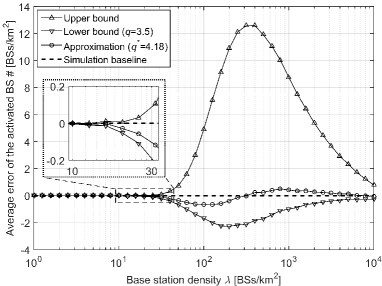
Fig. 2: Average error of the activated BS number ($\rho=300\,\textrm{UEs/km}^{2}$).

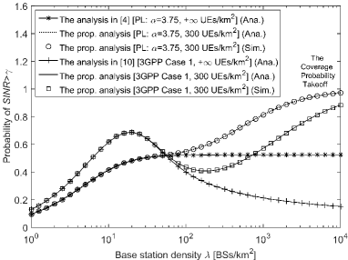
Fig. 3: $p^{\textrm{cov}}\left(\lambda,\gamma\right)$ vs. $\lambda$ with $\gamma=0\,\textrm{dB}$ and $q^{*}=4.18$.

In this section, we investigate the network performance and use numerical results to validate the accuracy of our analysis.

As a special case of Theorem 1, following [10], we consider a two-piece path loss and a linear LoS probability functions defined by the 3GPP [5], [6]. Specifically, in the path loss model presented in (1), we use $N=2$, $\zeta_{1}^{\textrm{L}}\left(w\right)=\zeta_{2}^{\textrm{L}}\left(w\right)=A^{{\rm{L}}}w^{-\alpha^{{\rm{L}}}}$, and $\zeta_{1}^{\textrm{NL}}\left(w\right)=\zeta_{2}^{\textrm{NL}}\left(w\right)=A^{{\rm{NL}}}w^{-\alpha^{{\rm{NL}}}}$ [5]. Moreover, in the LoS probability model shown in (4), we use $\textrm{Pr}_{1}^{\textrm{L}}\left(w\right)=1-\frac{w}{d_{1}}$ and $\textrm{Pr}_{2}^{\textrm{L}}\left(w\right)=0$, where $d_{1}$ is a constant [6]. For clarity, this 3GPP special case is referred to as 3GPP Case 1. As justified in [10], we use 3GPP Case 1 for the case study because it provides tractable results for (9)-(16) in Theorem 1.

Following [9, 10], we adopt the following parameters for 3GPP Case 1: $d_{1}=300$ m, $\alpha^{{\rm{L}}}=2.09$, $\alpha^{{\rm{NL}}}=3.75$, $A^{{\rm{L}}}=10^{-10.38}$, $A^{{\rm{NL}}}=10^{-14.54}$, $P=24$ dBm, $P_{{\rm{N}}}=-95$ dBm. Besides, the UE density is set to $\rho=300\thinspace\textrm{UEs/km}^{2}$.

To check the impact of different path loss models on our conclusions, we have also investigated the results for a single-slope path loss model that does not differentiate LoS and NLoS transmissions [4] where only one path loss exponent $\alpha$ is defined, the value of which is assumed to be $\alpha=\alpha^{{\rm{NL}}}=3.75$. Note that in this single-slope path loss model, the activated BS density is assumed to be $\lambda_{0}\left(3.5\right)$ shown in (21) [11].

IV-A Discussion on the Value of $q^{*}$ for the Approximate $\tilde{\lambda}$

Considering 3GPP Case 1 and Proposition 4, we conduct simulations to numerically find the optimal $q^{*}$ for the approximate $\tilde{\lambda}$. Based on the minimum mean squared error (MMSE) criterion, we obtain $q^{*}=4.18$. Fig. 2 shows the average errors of the number of activated BS for $\tilde{\lambda}^{{\rm{UB}}}$, $\tilde{\lambda}^{{\rm{LB}}}$, and $\lambda_{0}\left(q^{*}\right)$. Note that in Fig. 2 all results are compared against the simulation results, which create baseline results with zero errors. We can draw the following conclusions from Fig. 2:

• The proposed upper bound $\tilde{\lambda}^{{\rm{UB}}}$ and lower bound $\tilde{\lambda}^{{\rm{LB}}}$ are valid compared with the simulation results, i.e., $\tilde{\lambda}^{{\rm{UB}}}$ and $\tilde{\lambda}^{{\rm{LB}}}$ are always larger and smaller than the simulation baseline results, respectively.

• $\tilde{\lambda}^{{\rm{UB}}}$ is tighter than $\tilde{\lambda}^{{\rm{LB}}}$ when $\lambda$ is relatively small, e.g., $\lambda\in\left[10,30\right]\,\textrm{BSs/km}^{2}$.

• $\tilde{\lambda}^{{\rm{LB}}}$ is much tighter than $\tilde{\lambda}^{{\rm{UB}}}$ for dense and ultra-dense SCNs, e.g., $\lambda>100\,\textrm{BSs/km}^{2}$.

• The maximum error associated with $\lambda_{0}\left(q^{*}\right)$ is around $\pm$0.5 $\textrm{BSs/km}^{2}$, which is smaller than that of $\tilde{\lambda}^{{\rm{LB}}}$, e.g., an error around -2 $\textrm{BSs/km}^{2}$ when $\lambda=100\,\textrm{BSs/km}^{2}$.

IV-B Validation of Theorem 1 on the Coverage Probability

Fig. 3 shows the results of $p^{\textrm{cov}}\left(\lambda,\gamma\right)$ with $\gamma=0\,\textrm{dB}$ and $q^{*}=4.18$ plugged into Proposition 4. As one can observe, our analytical results given by Theorem 1 match the simulation results very well, which validates the accuracy of our analysis. In fact, Fig. 3 is essentially the same as Fig. 1 with the same marker styles, except that the results for the single-slope path loss model with $\rho=300\,\textrm{UEs/km}^{2}$ are also plotted. Fig. 3 confirms the key observations presented in Section I:

• For the single-slope path loss with $\rho=+\infty\,\textrm{UEs/km}^{2}$, the coverage probability approaches a constant for dense SCNs [4].

• For 3GPP Case 1 with $\rho=+\infty\,\textrm{UEs/km}^{2}$, the coverage probability decreases as $\lambda$ increases when the network is dense enough, i.e., $\lambda>20\,\textrm{BSs/km}^{2}$, due to the NLoS to LoS transition of interfering paths [10]. When $\lambda$ is very large, i.e., $\lambda\geq 10^{3}\,\textrm{BSs/km}^{2}$, the coverage probability decreases at a slower pace because both the interference and the signal powers are LoS dominated [10].

• For both path loss models with $\rho=300\,\textrm{UEs/km}^{2}$, the coverage probability performance continuously increases toward one in dense SCNs due to the IMCs, i.e., the Coverage Probability Takeoff, as discussed in Section I.

IV-C The Theoretical Results of the ASE

In Fig. 4, we show the results of $A^{\textrm{ASE}}\left(\lambda,\gamma_{0}\right)$ with $\gamma_{0}=0\,\textrm{dB}$ and $q^{*}=4.18$ plugged into Proposition 4. We can draw the following conclusions from Fig. 4:

• For the 3GPP Case 1 with $\rho=+\infty\,\textrm{UEs/km}^{2}$, the ASE suffers from a slow growth when $\lambda\in\left[20,200\right]\,\textrm{BSs/km}^{2}$ because of the interference transition from NLoS to LoS [10]. After that BS density region, for both path loss models with the IMC and $\rho=300\,\textrm{UEs/km}^{2}$, the ASEs monotonically grow as $\lambda$ increases in dense SCNs, but with performance gaps with regards to those of $\rho=+\infty\,\textrm{UEs/km}^{2}$ due to the finite number of UEs.

• The takeaway message should not be that the IMC generates an inferior ASE in dense SCNs. Instead, as explained in Section I, since there is a finite number of UEs in the network, some BSs are put to sleep and thus the spectrum reuse and in turn the area spectral efficiency decreases. However, the per-UE performance should increase as indicated by the probability of coverage shown in Fig. 3.

• Moreover, the IMC can greatly improve the SCN energy efficiency, i.e., the ratio of the ASE over the total energy consumption, which will be investigated in our future work considering practical power models for various levels of IMCs [3].

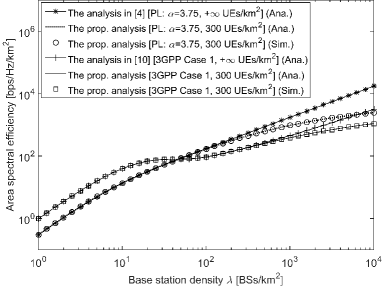
Fig. 4: $A^{\textrm{ASE}}\left(\lambda,\gamma_{0}\right)$ vs. $\lambda$ with $\gamma_{0}=0\,\textrm{dB}$ and $q^{*}=4.18$.

V Conclusion

In this paper, we have studied the impact of the IMC on the network performance in dense SCNs with LoS and NLoS transmissions. The impact is significant, i.e., as the BS density surpasses the UE density, the coverage probability will continuously increase toward one in dense SCNs (the Coverage Probability Takeoff), addressing the issue caused by the NLoS to LoS transition of interfering paths.

References

- [1] CISCO, “Cisco visual networking index: Global mobile data traffic forecast update (2013-2018),” Feb. 2014.
- [2] 3GPP, “TR 36.872: Small cell enhancements for E-UTRA and E-UTRAN - Physical layer aspects,” Dec. 2013.
- [3] D. L pez-P rez, M. Ding, H. Claussen, and A. Jafari, “Towards 1 Gbps/UE in cellular systems: Understanding ultra-dense small cell deployments,” IEEE Communications Surveys Tutorials, vol. 17, no. 4, pp. 2078–2101, Jun. 2015.
- [4] J. Andrews, F. Baccelli, and R. Ganti, “A tractable approach to coverage and rate in cellular networks,” IEEE Transactions on Communications, vol. 59, no. 11, pp. 3122–3134, Nov. 2011.
- [5] 3GPP, “TR 36.828: Further enhancements to LTE Time Division Duplex (TDD) for Downlink-Uplink (DL-UL) interference management and traffic adaptation,” Jun. 2012.
- [6] Spatial Channel Model AHG, “Subsection 3.5.3, Spatial Channel Model Text Description V6.0,” Apr. 2003.
- [7] X. Zhang and J. Andrews, “Downlink cellular network analysis with multi-slope path loss models,” IEEE Transactions on Communications, vol. 63, no. 5, pp. 1881–1894, May 2015.
- [8] T. Bai and R. Heath, “Coverage and rate analysis for millimeter-wave cellular networks,” IEEE Transactions on Wireless Communications, vol. 14, no. 2, pp. 1100–1114, Feb. 2015.
- [9] M. Ding, D. L pez-P rez, G. Mao, P. Wang, and Z. Lin, “Will the area spectral efficiency monotonically grow as small cells go dense?” IEEE GLOBECOM 2015, pp. 1–7, Dec. 2015.
- [10] M. Ding, P. Wang, D. L pez-P rez, G. Mao, and Z. Lin, “Performance impact of LoS and NLoS transmissions in dense cellular networks,” IEEE Transactions on Wireless Communications, vol. 15, no. 3, pp. 2365–2380, Mar. 2016.
- [11] S. Lee and K. Huang, “Coverage and economy of cellular networks with many base stations,” IEEE Communications Letters, vol. 16, no. 7, pp. 1038–1040, Jul. 2012.
- [12] Z. Luo, M. Ding, and H. Luo, “Dynamic small cell on/off scheduling using stackelberg game,” IEEE Communications Letters, vol. 18, no. 9, pp. 1615–1618, Sept 2014.
- [13] C. Li, J. Zhang, and K. Letaief, “Throughput and energy efficiency analysis of small cell networks with multi-antenna base stations,” IEEE Transactions on Wireless Communications, vol. 13, no. 5, pp. 2505–2517, May 2014.
- [14] R. L. Burden and J. D. Faires, Numerical Analysis (3rd Ed.). PWS Publishers, 1985.