Properties of interstellar dust responsible for extinction laws with unusually
low total-to-selective extinction ratios of $R_{V}=1$–2

Abstract

It is well known that the extinction properties along lines of sight to Type Ia supernovae (SNe Ia) are described by steep extinction curves with unusually low total-to-selective extinction ratios of $R_{V}=$ 1.0–2.0. In order to reveal the properties of interstellar dust that causes such peculiar extinction laws, we perform the fitting calculations to the measured extinction curves by applying a two-component dust model composed of graphite and silicate. As for the size distribution of grains, we consider two function forms of the power-law and lognormal distributions. We find that the steep extinction curves derived from the one-parameter formula by Cardelli et al. (1989) with $R_{V}=2.0$, $1.5$, and $1.0$ can be reasonably explained even by the simple power-law dust model that has a fixed power index of $-3.5$ with the maximum cut-off radii of $a_{\rm max}\simeq$ 0.13 $\mu$m, 0.094 $\mu$m, and 0.057 $\mu$m, respectively. These maximum cut-off radii are smaller than $a_{\rm max}\simeq 0.24$ $\mu$m considered to be valid in the Milky Way, clearly demonstrating that the interstellar dust responsible for steep extinction curves is highly biased to smaller sizes. We show that the lognomal size distribution can also lead to good fits to the extinction curves with $R_{V}=$ 1.0–3.1 by taking the appropriate combinations of the relevant parameters. We discuss that the extinction data at ultraviolet wavelengths are essential for constraining the composition and size distribution of interstellar dust.

1 Introduction

The reddening of Type Ia supernovae (SNe Ia) by dust grains is one of the largest uncertainties that limit the current precision of the cosmological parameters (e.g., Nordin et al., 2008). The reddening laws along lines of sight to SNe Ia are generally measured through the total-to-selective extinction ratio $R_{V}\equiv A_{V}/(A_{B}-A_{V})$, where $A_{V}$ and $A_{B}$ are the extinction in $V$ and $B$ bands, respectively. From the analyses of numerous samples of SNe Ia, many studies suggest that, to minimize the residual on the Hubble diagram, $R_{V}$ toward SNe Ia must be in a range of $R_{V}=$ 1.0–2.0 (e.g., Conley et al., 2007; Sullivan, 2010; Lampeitl et al., 2010), which is considerably lower than the range $R_{V}=$ 2.2–5.5 measured in the Milky Way (MW). The origin of such unusually low $R_{V}$ thus has been an important issue to be resolved for the applicability of SNe Ia as the cosmic standard candles.

The multi-band observations of individual SNe Ia also seem to commonly show the values as low as $R_{V}\leq\sim 2.0$ (Howell, 2011, and reference therein), although there is one study suggesting that weakly reddened SNe Ia have the values similar to the average $R_{V}=3.1$ in the MW (Folatelli et al., 2010). For these nearby SNe Ia, not only $R_{V}$ but also the extinction curves, namely the wavelength-dependence of extinction, can be obtained from optical to near-infrared photometries and spectra. The derived extinction curves are much steeper than the MW average extinction curve and are nicely fitted with the one-parameter formula given in Cardelli et al. (1989) by taking $R_{V}\simeq$ 1.0–2.0. Such non-standard extinction laws indicate that the properties of interstellar dust in host galaxies of SNe Ia are different from those in the MW or that other environmental effects associated with SNe Ia affect the apparent shapes of extinction curves.

One of the possible processes that have been suggested as provoking the steep extinction curves is the multiple scattering by dust grains surrounding SNe Ia; it has been shown that multiple scattering of photons in a circumstellar dust shell with a visual optical depth of $\tau\simeq 1.0$ can substantially steepen the extinction curve (Wang, 2005; Goobar, 2008; Amanullah & Goobar, 2011, but see also Nagao, Maeda, & Nozawa, 2016). However, if there exist such a moderately optically thick dust shell, we also expect thermal emission from the circumstellar dust that is heated by the SN radiation (so-called infrared light echo). Johansson et al. (2013) observed three nearby SNe Ia with Herschel but did not detect any far-infrared emission. Johansson et al. (2014) also reported the non-detection with Spitzer at 3.6 $\mu$m and 4.5 $\mu$m for several SNe Ia and placed the mass limit of $\leq$ $\sim 10^{-5}$ $M_{\odot}$ on the amount of the circumstellar dust. Furthermore, by comparing an infrared light echo model and near-infrared observations of SNe Ia samples, Maeda et al. (2015) put the upper limits of $\tau_{B}\leq\sim 0.1$ on the $B$-band optical depths of circumstellar dust shells. These works point out that there would not be massive dust shells around SNe Ia so that the multiple scattering by local dust might not be a valid explanation of the unusual extinction laws.

Recently, Type Ia SN 2014J was discovered in the starburst galaxy M82 at a distance of $\simeq$ 3.5 Mpc (Dalcanton et al., 2009), which is the nearest among SNe Ia reported in the last thirty years. This SN is highly reddened and thus offer the best opportunity to study the extinction property on its sightline. The extensive observations have revealed that the extinction curve derived for SN 2014J is highly steep with a very low value of $R_{V}\simeq 1.5$ (e.g., Goobar et al., 2014; Amanullah et al., 2014; Foley et al., 2014; Marion et al., 2015). From a simultaneous fit to the extinction and polarization data, Hoang (2015) claim that both interstellar and circumstellar dust are responsible for the anomalous extinction property toward SN 2014J. However, the time invariability of the color (Brown et al., 2015) and polarization (Kawabata et al., 2014; Patet et al., 2015) indicates that its peculiar extinction is mainly of interstellar-dust origin. This seems to be also supported by non-detection of infrared excess, which otherwise would be caused by the circumstellar dust shell around SN 2014J (Johansson et al., 2014; Telesco et al., 2015).

These studies above provide an increasing number of evidence that the unusual extinction curves toward SNe Ia are likely to be originated by interstellar dust in their host galaxies. Hence, the extinction curves measured for SNe Ia can be powerful tools for probing the properties of interstellar dust in external galaxies. In general, a low $R_{V}$ is interpreted as corresponding to a smaller average radius of dust than that in the MW. Gao et al. (2015) searched for a physical model of relevant dust grains via the fitting to the measured color-excess curve of SN 2014J and found that their size distribution is biased to small radii relative to that in the MW. However, it has not been systematically investigated how small the interstellar dust should be, to produce the steep extinction curves appeared for SNe Ia. As stated above, the extinction laws toward SNe Ia are well described by the extinction curves derived from the empirical formula by Cardelli et al. (1989) (which we, hereafter, refer to as the CCM curves). Therefore, in this paper, we aim to comprehensively understand what composition and size distribution of interstellar dust can reproduce the CCM curves with exceptionally low values of $R_{V}\leq 2.0$.

The paper is organized as follows. In Section 2, the procedure of the fitting calculations and the model of dust used for deriving the extinction curves are described. The results of the calculations are presented in Section 3 and discussed in Section 4. In Section 5, our main conclusions are remarked. Throughout this paper, dust grains are assumed to be spherical.

2 Fitting model of extinction curves

2.1 Data on extinction curves

The main aim of this study is to explore how a variety of the CCM curves described by different $R_{V}$ can translate to the properties of interstellar dust. In order to do this, we perform the calculations of fitting to the CCM curves by applying a simple dust model. However, we do not try to fit the whole shape of the CCM curve by finely spacing wavelengths from 0.125 $\mu$m to 3.5 $\mu$m under consideration. Indeed, the continuous CCM curves have been derived by interpolating the data of extinction obtained from ultraviolet (UV) spectra and optical to near-infrared photometries (Cardelli et al., 1989). Given that the extinction curves are usually extracted on the basis of photometric observations, it is practical to consider the extinction at the specific wavelengths where the observational data are available. In this study, we take, as the reference wavelengths, the effective wavelengths of widely-used optical to near-infrared photometric filters and wide-band UV photometric filters onboard representative satellites such as Habble Space Telescope (HST), GALEX, and Swift. Table 1 presents the reference wavelengths $\lambda_{i}$ adopted in this study. At these wavelengths, we calculate the extinction values $A_{\lambda_{i}}/A_{V}$ normalized to that in $V$ band for different $R_{V}$ by means of the CCM formula and use them as the data of extinction curves to be fitted.

Table 1: Reference wavelengths adopted in this study.

Wavelength $\lambda_{i}$	$1/\lambda_{i}$	$\sigma_{i}$ a	Photometric filters	References b
($\mu$m)	($\mu$m-1)
0.125	8.000	0.32*	—
0.1528	6.545	0.19*	FUV (GALEX)	(1)
0.1928	5.187	0.15*	uvw2 (Swift)	(2)
0.2224	4.496	0.2*	F218W (HST), NUV (GALEX) c	(3), (1)
0.2359	4.239	0.2	F225W (HST)	(3)
0.26	3.846	0.12*	uvw1 (Swift)	(2)
0.2704	3.698	0.12	F275W (HST)	(3)
0.3355	2.981	0.065*	F336W (HST)	(3)
0.3531	2.832	0.065	$u$ band	(4)
0.365	2.740	0.022*	$U$ band
0.3921	2.550	0.022	F390W (HST)	(3)
0.44	2.273	0.02*	$B$ band
0.4627	2.161	0.02	$g$ band	(4)
0.55	1.818	—	$V$ band
0.614	1.629	0.02	$r$ band	(4)
0.66	1.515	0.02*	$R_{\rm c}$ band
0.7467	1.339	0.02	$i$ band	(4)
0.81	1.235	0.027	$I_{\rm c}$ band
0.8887	1.125	0.027*	$z$ band	(4)
1.25	0.800	0.03*	$J$ band	(5)
1.65	0.606	0.034*	$H$ band	(5)
2.16	0.463	0.04*	$K_{s}$ band	(5)
3.4	0.294	0.06*	$L$ band

^aThe uncertainties of extinction $(A_{\lambda_{i}}/A_{V})_{\rm CCM}$ obtained from the CCM formula at the reference wavelengths $\lambda_{i}$. The values marked by asterisks are taken from Cardelli et al. (1989), while the others are deduced from those at the adjacent reference wavelengths.
^bReferences for the wavelengths: (1) Morrissey et al. (2005), (2) Poole et al. (2008), (3) Dressel (2016), (4) 2.5 m reference in Doi et al. (2010), (5) 2MASS bands in Skrutskie et al. (2006).
^cFor the GALEX NUV band, the effective wavelength is 0.2271 $\mu$m.

2.2 Model of interstellar dust

For the model of interstellar dust, we adopt a two-component model consisting of graphite and silicate. As for the size distribution of dust, we consider two simple function forms: one is the power-law size distribution given as

$$n_{j}(a)=C_{j}f_{j}(a)=C_{j}a^{-q_{j}},$$ (1)

where $n_{j}(a)da$ is the number density of grain species $j$ ($j$ denotes graphite or silicate) with radii between $a$ and $a+da$. The normalization factor $C_{j}$ is related to the specific mass of dust grains, $m_{j}$, as

$$C_{j}=m_{j}\left(\frac{4\pi\rho_{j}}{3}\int_{a_{{\rm min},j}}^{a_{{\rm max},j}}a^{3}f_{j}(a)da\right)^{-1}=\frac{m_{j}}{X_{j}},$$ (2)

with $\rho_{j}$ being the material density ($\rho_{\rm gra}=2.24$ g cm^-3 and $\rho_{\rm sil}=3.3$ g cm^-3), $a_{{\rm max},j}$ the maximum cut-off radius, and $a_{{\rm min},j}$ the minimum cut-off radius of grain species $j$. It is well known that, for this grain composition and size distribution function, the average extinction curve in the MW is nicely reproduced by taking $q_{\rm gra}=q_{\rm sil}=3.5$, $a_{\rm max,gra}=a_{\rm max,sil}\simeq 0.25$ $\mu$m, $a_{\rm min,gra}=a_{\rm min,sil}\simeq 0.005$ $\mu$m, which has been referred to as the MRN dust model (Mathis et al., 1977; Draine & Lee, 1984). Note that the power-law distribution is originated from the collisional fragmentation of dust grains (Biermann & Harwit, 1980), which is considered as one of the main physical processes that modulate the size distribution of interstellar dust (e.g., Hirashita & Nozawa, 2013; Asano et al., 2013).

On the other hand, the size distributions of dust produced in stellar sources would not necessarily follow the power-law distribution; it has been suggested that the size distributions of dust ejected from core-collapse supernovae (CCSNe) and asymptotic giant branch (AGB) stars are lognormal-like with peaks around 0.1–1.0 $\mu$m (e.g., Nozawa et al., 2007; Yasuda & Kozasa, 2012). Hence, as the other size distribution function, we adopt the lognormal form of

$$n_{j}(a)=C_{j}f_{j}(a)=\frac{C_{j}}{\sqrt{2\pi}a\gamma_{j}}\exp\left[-\frac{(\ln a-\ln a_{0,j})^{2}}{2\gamma_{j}^{2}}\right],$$ (3)

where $a_{0,j}$ and $\gamma_{j}$ are the characteristic grain radius and the standard deviation of the lognormal distribution, respectively. The normalization factor $C_{j}$ in Equation (3) is also determined from Equation (2), for which we fix $a_{{\rm max},j}=10$ $\mu$m and $a_{{\rm min},j}=5\times 10^{-4}$ $\mu$m.

There are some elaborate interstellar dust models that consider various grain components and more complicated functional forms for grain size distributions (e.g., Weingartner & Draine, 2001; Clayton et al., 2003; Zubko et al., 2004; Jones et al., 2013). These dust models are tailored to produce excellent fits to the average MW extinction curve and to meet the constraints on elemental abundances in the interstellar medium. However, the information on elemental abundances is poorly available in general, especially for host galaxies of SNe Ia. Thus, we do not take into account the abundance constraints in the present analysis and address only the reproduction of wavelength dependence of extinction. Furthermore, our goal is to grasp the systematic behavior of how the properties of dust vary according to the extinction curves, not to seek a unique set of the grain composition and size distribution that gives the best fit to each extinction curve. For this purpose, the simple dust models as proposed here are favorable, and they may also be useful to illustrate the applicability of the power-law and lognormal size distributions.

Under the assumption that both graphite and silicate grains are uniformly distributed in interstellar space, the extinction curve $A_{\lambda}/A_{V}$ is calculated, for the dust model described above, as

$$\frac{A_{\lambda}}{A_{V}}=\frac{\sum_{j}K_{j}\int_{a_{{\rm min},j}}^{a_{{\rm max},j}}\pi a^{2}f_{j}(a)Q_{\lambda,j}^{\rm ext}(a)da}{\sum_{j}K_{j}\int_{a_{{\rm min},j}}^{a_{{\rm max},j}}\pi a^{2}f_{j}(a)Q_{V,j}^{\rm ext}(a)da},$$ (4)

where

$$K_{\rm gra}=\frac{C_{\rm gra}}{C_{\rm sil}}=f_{\rm gs}\left(\frac{X_{\rm sil}}{X_{\rm gra}}\right)~{}~{}~{}{\rm and}~{}~{}~{}K_{\rm sil}=1$$ (5)

with the mass ratio $f_{\rm gs}=m_{\rm gra}/m_{\rm sil}$ of graphite to silicate. The extinction coefficients $Q_{\lambda,j}^{\rm ext}(a)$ are calculated with Mie scattering from dielectric constants for graphite and astronomical silicate (which we refer to simply as silicate in what follows) in Draine & Lee (1984) and Draine (2003). In computing $Q_{\lambda,j}^{\rm ext}$ for graphite, the $1/3$–$2/3$ approximation is employed to take the anisotropy into consideration (Draine & Malhotra, 1993).

For the power-law size distribution, there are seven adjustable parameters: $f_{\rm gs}$, which prescribes the mixture of graphite and silicate grains, and $q_{\rm gra}$, $q_{\rm sil}$, $a_{\rm max,gra}$, $a_{\rm max,sil}$, $a_{\rm min,gra}$, and $a_{\rm min,sil}$, which regulate the size distribution of each grain species. As discussed in Nozawa & Fukugita (2013), $a_{{\rm min},j}$ cannot be constrained very much unless the extinction data at wavelengths shorter than $\simeq$0.1 $\mu$m are used. Therefore, we fix $a_{{\rm min},j}=0.005$ $\mu$m for both graphite and silicate. For this power-law distribution, we consider five dust models, depending on the combinations of the free parameters and fixed parameters, as summarized in Table 2. For example, the dust model in which graphite and silicate have the same size distribution with $q=q_{\rm gra}=q_{\rm sil}=3.5$ and $a_{\rm max}=a_{\rm max,gra}=a_{\rm max,sil}$ is referred to as Model 1. On the other hand, the dust model in which all of $f_{\rm gs}$, $q_{\rm gra}$, $q_{\rm sil}$, $a_{\rm max,gra}$, and $a_{\rm max,sil}$ are treated as free parameters is referred to as Model 5. Hereafter, we mainly show the results of the fitting calculations for Model 1. This simple dust model reduces the number of parameters to only two ($f_{\rm gs}$ and $a_{\rm max}$) and can be regarded as a natural extention of the MRN dust model.

For the lognormal size distribution, the adjustable parameters are $f_{\rm gs}$, $a_{\rm 0,gra}$, $a_{\rm 0,sil}$, $\gamma_{\rm gra}$, and $\gamma_{\rm sil}$. For this size distribution, two dust models are considered, according to the numbers of the free parameters. The details of the dust models for the lognormal size distribution are given in Table 3 and are described in Section 3.2.

2.3 Fitting procedure

We carry out the fitting through comparison between the extinction data and the calculated extinction $y_{{\rm cal},i}=(A_{\lambda_{i}}/A_{V})_{\rm cal}$ at each reference wavelength $\lambda_{i}$. The goodness of the fitting is evaluated by $\chi^{2}$, which might be, for instance, given as

$$\chi_{0}^{2}=\frac{\langle\sigma\rangle^{2}}{N_{\rm data}-N_{\rm para}}\sum_{i}^{N_{\rm data}}\frac{\left(y_{{\rm CCM},i}-y_{{\rm cal},i}\right)^{2}}{\sigma_{i}^{2}},$$ (6)

where $y_{{\rm CCM},i}=(A_{\lambda_{i}}/A_{V})_{\rm CCM}$ is the extinction derived from the CCM formula at $\lambda_{i}$, $N_{\rm data}$ is the number of the data to be fitted (i.e., the number of the reference wavelengths under consideration except for $V$ band), $N_{\rm para}$ is the number of free parameters, $\sigma_{i}$ are weights, and $\langle\sigma\rangle^{2}=[(1/N_{\rm data})\sum_{i}^{N_{\rm data}}(1/\sigma_{i}^{2})]^{-1}$ is the adjustment coefficient for alleviating the large external errors arising from $\sigma_{i}^{2}$. As for $\sigma_{i}$, which are generally assigned as the uncertainties of observational data (e.g., Gao et al., 2015), we take the standard deviation of $A_{\lambda}/A_{V}$ given in Table 2 of Cardelli et al. (1989). For $\sigma_{i}$ not given in Cardelli et al. (1989), we infer their values from those at the closest reference wavelengths. The adopted values of $\sigma_{i}$ are provided in Table 1.

It should be noted that a set of the best-fit parameters that minimizes $\chi_{0}^{2}$ in Equation (6) does not necessarily produce apparently good fits to the entire range of extinction curves; since $\sigma_{i}$ are considerably large at UV wavelengths (see Table 1), the data of UV extinction are unimportantly treated in the fitting calculations, resulting in poor fits at UV wavelengths. Therefore, as in some previous studies (e.g., Weingartner & Draine, 2001), we adopt an identical weight $\sigma_{i}=1$, independent of $\lambda_{i}$, and assess the dispersion by

$$\chi_{1}^{2}=\frac{1}{N_{\rm data}-N_{\rm para}}\sum_{i}^{N_{\rm data}}\left(y_{{\rm CCM},i}-y_{{\rm cal},i}\right)^{2}.$$ (7)

In the case that the extinction data at all the reference wavelengths covering UV to near-infrared are exploited, $N_{\rm data}=22$. In Section 4.2, we will also show the results of the fitting calculations in the cases that the extinction data at UV wavelengths are not taken into account.

Table 2: Dust models with power-law size distributions and their parameter sets.

Dust model	$N_{\rm para}$	free parameters	constraints$\,{}^{a}$
Model 1	2	$a_{\rm max}$, $f_{\rm gs}$	$q_{\rm gra}=q_{\rm sil}=3.5$, $a_{\rm max}=a_{\rm max,gra}=a_{\rm max,sil}$
Model 2	2	$q$, $f_{\rm gs}$	$q=q_{\rm gra}=q_{\rm sil}$, $a_{\rm max,gra}=a_{\rm max,sil}=0.25$ $\mu$m
Model 3	3	$a_{\rm max,gra}$, $a_{\rm max,sil}$, $f_{\rm gs}$	$q_{\rm gra}=q_{\rm sil}=3.5$
Model 4	3	$q$, $a_{\rm max,}$, $f_{\rm gs}$	$q=q_{\rm gra}=q_{\rm sil}$, $a_{\rm max}=a_{\rm max,gra}=a_{\rm max,sil}$
Model 5	5	$q_{\rm gra}$, $q_{\rm sil}$, $a_{\rm max,gra}$, $a_{\rm max,sil}$, $f_{\rm gs}$	—

^aFor all of the models here, the minimum cut-off radii are fixed as $a_{\rm min,gra}=a_{\rm min,sil}=0.005$ $\mu$m.

Table 3: Dust models with lognormal size distributions and their parameter sets.

Dust model	$N_{\rm para}$	free parameters	constraints$\,{}^{a}$
Model 1s	3	$a_{\rm 0,gra}$, $a_{\rm 0,sil}$, $f_{\rm gs}$	$\gamma_{\rm gra}=\gamma_{\rm sil}=0.5$
Model 5s	5	$a_{\rm 0,gra}$, $a_{\rm 0,sil}$, $\gamma_{\rm gra}$, $\gamma_{\rm sil}$, $f_{\rm gs}$	—

^aFor the models with lognormal size distributions, the maximum and minimum cut-off radii are fixed to be $a_{\rm max,gra}=a_{\rm max,sil}=10$ $\mu$m and $a_{\rm min,gra}=a_{\rm min,sil}=5\times 10^{-4}$ $\mu$m, respectively.

Table 4: A set of the best-fit parameters obtained for dust models with power-law size distributions.

Dust model$\,{}^{a}$	$q_{\rm gra}$	$a_{\rm max,gra}$	$q_{\rm sil}$	$a_{\rm max,sil}$	$f_{\rm gs}$	$\chi_{1}$	$R_{V}^{\rm cal}$
		($\mu$m)		($\mu$m)
$R_{V}^{\rm CCM}=3.1$
Model 1	3.50	0.243	3.50	0.243	0.57	0.0464	3.38
Model 2	3.53	0.250	3.53	0.250	0.60	0.0430	3.46
Model 3	3.50	0.119	3.50	0.544	0.25	0.0462	3.44
Model 4	3.58	0.274	3.58	0.274	0.60	0.0413	3.56
Model 5	3.78	0.471	3.42	0.290	0.44	0.0358	3.46
$R_{V}^{\rm CCM}=2.0$
Model 1	3.50	0.134	3.50	0.134	0.46	0.0932	2.16
Model 2	4.05	0.250	4.05	0.250	0.50	0.0893	2.66
Model 3	3.50	0.0386	3.50	0.270	0.16	0.0550	2.41
Model 4	3.84	0.174	3.84	0.174	0.49	0.0540	2.41
Model 5	4.04	0.164	3.76	0.230	0.35	0.0368	2.34
$R_{V}^{\rm CCM}=1.5$
Model 1	3.50	0.0944	3.50	0.0944	0.49	0.0707	1.75
Model 2	4.40	0.250	4.40	0.250	0.47	0.231	2.34
Model 3	3.50	0.0884	3.50	0.0735	0.64	0.0535	1.72
Model 4	3.67	0.102	3.67	0.102	0.48	0.0643	1.89
Model 5	4.10	0.0903	3.85	0.200	0.31	0.0465	1.74
$R_{V}^{\rm CCM}=1.0$
Model 1	3.50	0.0572	3.50	0.0572	0.60	0.223	1.49
Model 2	5.08	0.250	5.08	0.250	0.42	0.663	2.10
Model 3	3.50	0.0627	3.50	0.0844	0.42	0.171	1.39
Model 4	3.28	0.0546	3.28	0.0546	0.63	0.218	1.47
Model 5	3.86	0.0600	3.77	0.128	0.30	0.158	1.34

^aThe free parameters and constraints adopted in the power-law dust models are described in Table 2.

3 Results of fitting calculations

3.1 Extinction curves from dust models with power-law size distributions

We first consider the average MW extinction curve with $R_{V}^{\rm CCM}=3.1$ to check if our fitting method yields the plausible results. As mentioned above, this extinction curve can be well matched by the MRN dust model that is represented by the power-law size distribution with $q=3.5$ and $a_{\rm max}=0.25$ $\mu$m (Mathis et al., 1977; Draine & Lee, 1984; Nozawa & Fukugita, 2013). Thus, our fitting calculations should lead to the similar values for $q$ and $a_{\rm max}$.

The results of the fitting calculations are given in Table 4, which summarizes a set of parameters that give the best fit for each dust model with a power-law size distribution. For Model 1, which assumes $q=3.5$ and $a_{\rm max}=a_{\rm max,gra}=a_{\rm max,sil}$, the best fit is achieved with $a_{\rm max}=0.243$ $\mu$m and $f_{\rm gs}=0.57$. On the other hand, if we fix as $a_{\rm max}=0.25$ $\mu$m (Model 2), the power index $q=3.53$ offers the best fit with $f_{\rm gs}=0.60$. Hence, our simplest dust models (Models 1 and 2) present the results consistent with the MRN dust model, demonstrating that our fitting method works well.

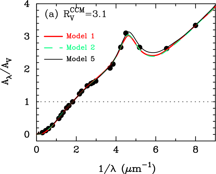
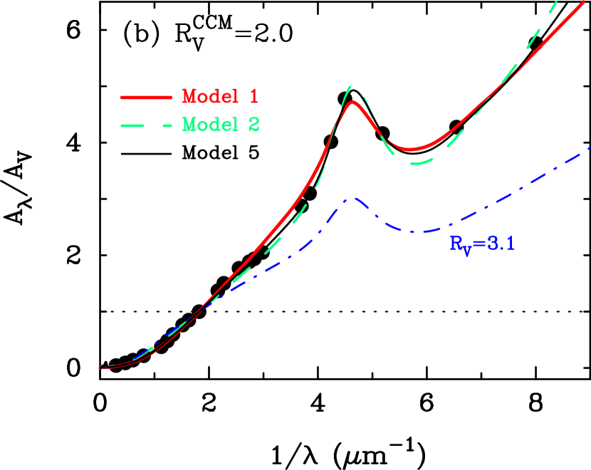
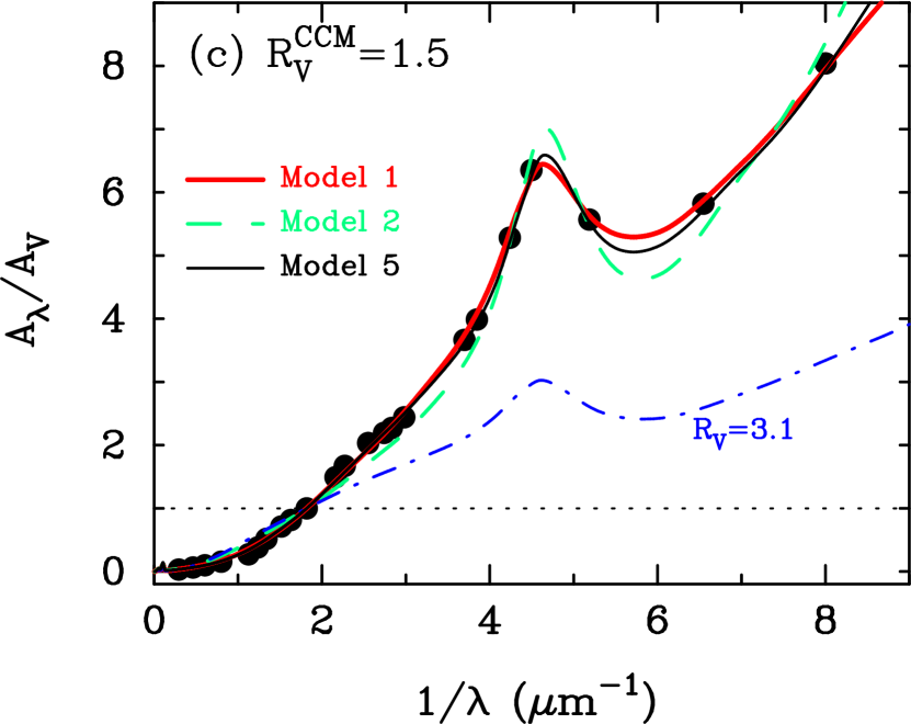
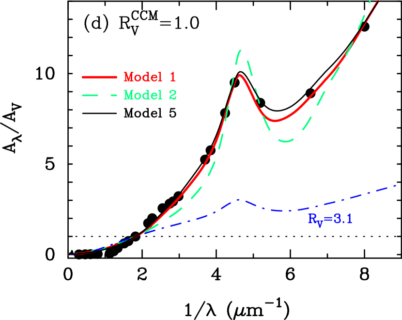
Figure 1: Extinction curves calculated from the best-fit parameters in Model 1 (thick solid), Model 2 (dashed), and Model 5 (thin solid) with power-law size distributions for (a) $R_{V}^{\rm CCM}=3.1$ (b) $2.0$, (c) $1.5$, and (d) $1.0$. The filled circles are the extinction data at the reference wavelengths, derived from the CCM formula for each $R_{V}^{\rm CCM}$ value. For the panels (b)–(d), the extinction curve derived from Model 1 for $R_{V}^{\rm CCM}=3.1$ is shown by the dot-dashed line for reference.

The extinction curves derived from these best-fit parameters are shown in Figure 1(a). We can see that the extinction curves obtained from Model 1 and Model 2 are fully overlapped and reproduce the whole shape of the CCM curve with $R_{V}^{\rm CCM}=3.1$. In Figure 1(a), we also depict the extinction curve from Model 5. Since Model 5 treats the five quantities ($q_{\rm gra}$, $a_{\rm max,gra}$, $q_{\rm sil}$, $a_{\rm max,sil}$, and $f_{\rm gs}$) as free parameters, the best-fit values result in the least dispersion among the dust models considered for the power-law size distribution (see Table 4). However, as is observed from Figure 1(a), the match between the resulting extinction curve and the extinction data is not largely superior to that for Model 1. Given that Model 1 (and Model 2) gives a satisfactory fit despite its small number of free parameters, such a simplest dust model should be regarded as being instructive for understanding the properties of dust in comparison with the MRN model.

Next we search for the dust models that can account for very steep extinction curves with $R_{V}^{\rm CCM}\leq 2.0$. Figures 1(b), 1(c), and 1(d) show the results of the fitting to the CCM curves with $R_{V}^{\rm CCM}=2.0$, $1.5$, and $1.0$, respectively. For Model 1 with $q=3.5$ and $a_{\rm max,gra}=a_{\rm max,sil}$, the least dispersions are achieved with $a_{\rm max}=0.134$ $\mu$m, $0.0944$ $\mu$m, and $0.0572$ $\mu$m for $R_{V}^{\rm CCM}=2.0$, $1.5$, and $1.0$. For these cases, the mass ratio of graphite to silicate is in a range of $f_{\rm gs}=$ 0.45–0.6. The dispersions are considerably small for $R_{V}^{\rm CCM}=2.0$ and $1.5$, demonstrating that the fits are adequate. The fit to the $R_{V}^{\rm CCM}=1.0$ curve is not good very much at optical to near-infrared wavelengths, but the calculated extinction curve can roughly reproduce the entire wavelength-dependence of extinction.

In Figures 1(b)–1(d), we also plot the extinction curves calculated from the best-fit combination of $f_{\rm gas}$ and $q$ for Model 2. When the maximum cut-off radii are fixed as $a_{\rm max}=0.25$ $\mu$m, the optimum values of $q$ are 4.05, 4.40, and 5.08, respectively, for $R_{V}^{\rm CCM}=2.0$, $1.5$, and $1.0$. This implies that as the extinction curves become steeper, the steeper size distributions are required. However, as is obvious from Figures 1(c) and 1(d), the best-fit parameters for Model 2 lead to a poor match to the CCM curves with $R_{V}^{\rm CCM}=1.5$ and $1.0$. Therefore, only enhancement in $q$, with a fixed $a_{\rm max}$, is not sufficient for describing the highly steep extinction curves with $R_{V}^{\rm CCM}\leq 1.5$. Nevertheless, for $R_{V}^{\rm CCM}=2.0$, the size distribution from Model 2 with $q=4.05$ and $a_{\rm max}=0.25$ $\mu$m yields a better fit than that for Model 1 with $q=3.5$ and $a_{\rm max}=0.134$ $\mu$m.

These results indicate that the steeper extinction curves represented by the values as low as $R_{V}^{\rm CCM}=$ 1.0–2.0 can be explained by the dust model whose power-law size distribution is skewed to smaller radii than the MRN model. More specifically, if $a_{\rm max}=0.25$ $\mu$m is held, the power index is needed to be increased from $q\simeq 3.5$ for $R_{V}^{\rm CCM}=$ 3.1 up to $q\simeq$ 4.0 for $R_{V}^{\rm CCM}=$ 2.0. On the other hand, for $R_{V}^{\rm CCM}=$ 1.0–2.0, a better fit can be generally obtained through reducing the maximum cut-off radius by a factor of 2–5 in comparion to the MRN model, with a fixed index of $q=3.5$ and a mass ratio of $f_{\rm gs}=$ 0.45–0.6. Given the peculiality of the extinction curves as never appeared in the MW, the maximum cut-off radii of $a_{\rm max}\simeq$ 0.06–0.13 $\mu$m are not too small and thus may not be unrealistic. The important consequence of the present analysis is that the remarkably tilted extinction curves measured for SNe Ia can be described in the context of the simple dust model with the power-law size distribution.

Table 5: A set of the best-fit parameters obtained for dust models with lognormal size distributions.

Dust model$\,{}^{a}$	$\gamma_{\rm gra}$	$a_{\rm 0,gra}$	$\gamma_{\rm sil}$	$a_{\rm 0,sil}$	$f_{\rm gs}$	$\chi_{1}$	$R_{V}^{\rm cal}$
		($\mu$m)		($\mu$m)
$R_{V}^{\rm CCM}=3.1$
Model 1s	0.50	0.0358	0.50	0.0253	0.91	0.139	2.81
Model 5s	1.32	$5.05\times 10^{-4}$	1.34	$5.12\times 10^{-4}$	0.55	0.0675	3.56
$R_{V}^{\rm CCM}=2.0$
Model 1s	0.50	0.0238	0.50	0.0201	0.78	0.208	1.87
Model 5s	1.18	$5.60\times 10^{-4}$	1.25	$5.00\times 10^{-4}$	0.42	0.0608	2.48
$R_{V}^{\rm CCM}=1.5$
Model 1s	0.50	0.0186	0.50	0.0185	0.69	0.220	1.61
Model 5s	0.86	$2.84\times 10^{-3}$	1.06	$1.48\times 10^{-3}$	0.38	0.0890	1.95
$R_{V}^{\rm CCM}=1.0$
Model 1s	0.50	0.0127	0.50	0.0172	0.54	0.239	1.49
Model 5s	0.50	0.0114	0.71	$8.63\times 10^{-3}$	0.39	0.232	1.50

^aThe free parameters and constraints adopted in the lognormal dust models are described in Table 3.

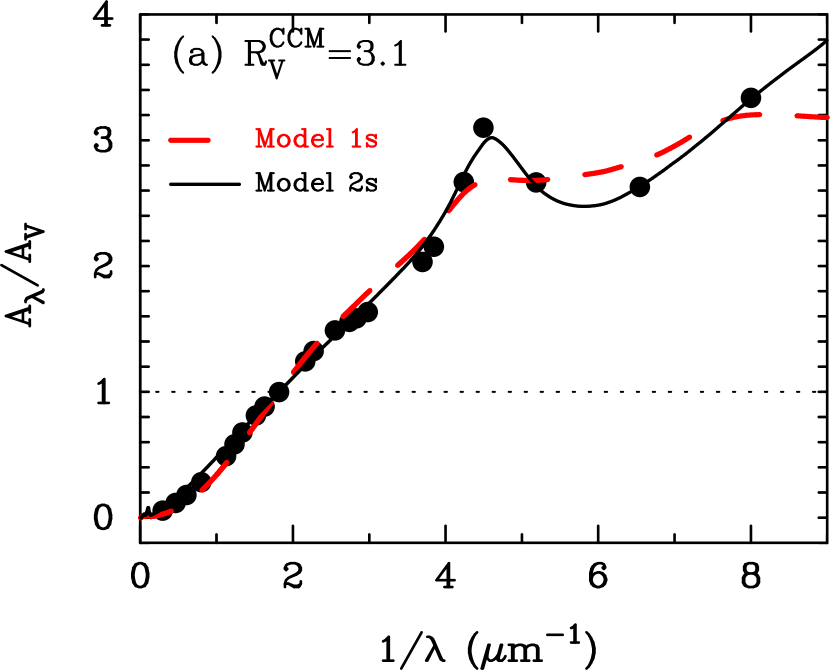
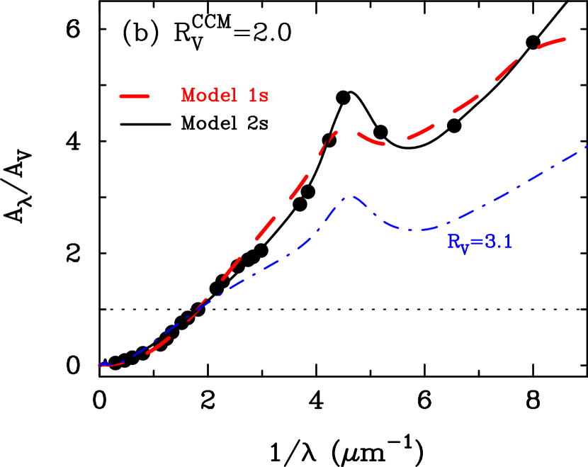
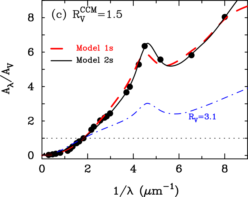
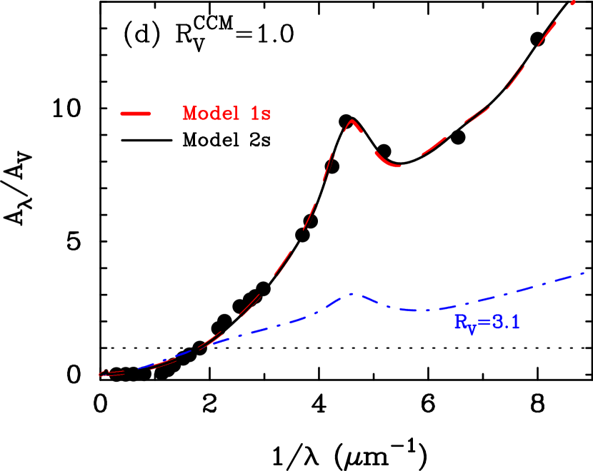
Figure 2: Extinction curves calculated from the best-fit parameters in Model 1s (dashed lines) and Model 5s (solid lines) with lognormal size distributions for (a) $R_{V}^{\rm CCM}=3.1$ (b) $2.0$, (c) $1.5$, and (d) $1.0$. The filled circles are the extinction data at the reference wavelengths, derived from the CCM formula for each $R_{V}^{\rm CCM}$ value. For the panels (b)–(d), the extinction curve derived from Model 1 with the power-law size distribution for $R_{V}^{\rm CCM}=3.1$ is shown by the dot-dashed line for reference.

3.2 Extinction curves from dust models with lognormal size distributions

In this section, we examine whether the dust models with lognormal size distributions can lead to the good fit to the CCM curves with $R_{V}^{\rm CCM}=$ 1.0–3.1. As mentioned in Section 2.2, the lognormal-like size distributions have been suggested as those of dust supplied from CCSNe and AGB stars. Hirashita et al. (2015) adopted the standard deviation of $\gamma_{j}=0.49$ for the lognormal size distribution of dust from these stellar sources. Following this study, we first consider the case with $\gamma_{j}=0.5$, treating $a_{\rm 0,gra}$, $a_{\rm 0,sil}$, and $f_{\rm gs}$ as parameters (referred to as Model 1s). We note that $\gamma_{j}=0.5$ presents a well peaked distribution, so such lognormal distributions would be useful to seek the characteristic grain radius responsible for the measured extinction curves.

The best-fit parameters from the fitting calculations for lognormal grain size distributions are given in Table 5. For a fixed value of $\gamma_{j}=0.5$, the best-fits are obtained with $a_{0,j}\simeq 0.03$ $\mu$m (for $R_{V}^{\rm CCM}=$ 3.1) down to $a_{0,j}\simeq 0.01$ $\mu$m (for $R_{V}^{\rm CCM}=$ 1.0), indicating that the characteristic grain radius decreases as the extinction curve becomes steeper. However, as shown by dashed lines in Figure 2, the matches are poor, especially for $R_{V}^{\rm CCM}=$ 3.1, 2.0, and 1.5. Hence,the lognormal distribution with the standard deviation as low as $\gamma_{j}=0.5$ is not likely to be suitable for managing these steep CCM curves.

On the other hand, if we treat all of the five quantities ($f_{\rm gs}$, $a_{\rm 0,gra}$, $a_{\rm 0,sil}$, $\gamma_{\rm gra}$, and $\gamma_{\rm sil}$) involved in the lognormal distribution as free parameters (referred to as Model 5s), the nice fits are obtained (solid lines in Figure 2); in the case of Model 5s, $a_{0,j}\leq\sim 3\times 10^{-3}$ $\mu$m and $\gamma_{j}\simeq 1.0$ are necessary for producing the good fits to the extinction curves with $R_{V}^{\rm CCM}=$ 3.1, 2.0, and 1.5. Note that the size distribution obtained from such a small $a_{0,j}$ and a large $\gamma_{j}$ can be viewed as an exponential-like distribution rather than a lognormal distribution with a sharp peak (see Figure 3). For $R_{V}^{\rm CCM}=$ 1.0, a peaked lognormal distribution seems to yield the entire agreement with the extinction data, although the match is not necessarily sufficient in optical and near-infrared regions.

The inspection of Figure 3 allows us to point out that the size distributions offering the best-fits for Model 5s have well similar slopes to the corresponding power-law distributions at the radii between $\simeq$0.01 $\mu$m and $\simeq$0.2 $\mu$m. Then, we see if this similarity also holds with regard to the average radii given as

$$\langle a_{{\rm ave},j}^{m}\rangle=\left(\frac{\int_{a_{{\rm min},j}}^{a_{{\rm max},j}}a^{m}n(a)da}{\int_{a_{{\rm min},j}}^{a_{{\rm max},j}}n(a)da}\right)^{\frac{1}{m}}~{}~{}~{}~{}(m=1,2,3).$$ (8)

Table 6 presents the average radii from the best-fit parameters for some of the dust models in this study. We can see that $\langle a_{{\rm ave},j}^{m}\rangle$ from Models 5 and 5s do not coincide at all, despite the fact that their size distributions highly resemble at $a\simeq$ 0.01–0.2 $\mu$m. For $R_{V}^{\rm CCM}=$ 3.1, 2.0, and 1.5, $\langle a_{{\rm ave},j}^{m}\rangle$ from Model 5s are always smaller than those from Model 5. This is because $a_{{\rm min},j}$ (and $a_{0,j}$) in Model 5s is much smaller than $a_{{\rm min},j}=0.005$ $\mu$m in Model 5. Meanwhile, $\langle a_{{\rm ave},j}^{m}\rangle$ is higher in Model 5s for $R_{V}^{\rm CCM}=$ 1.0 due to the lack of grains smaller than $\simeq$0.01 $\mu$m. Hence, it would not be proper to invoke the average radius when the properties of dust are discussed in the context of extinction curves. Indeed, the radii of grains which mainly contribute to extinction are different at different wavelengths, so the wavelength-dependence of extinction could not be described only with a single characteristic grain radius.

We have revealed that the lognormal size distribution can lead to good fits to the CCM curves with $R_{V}^{\rm CCM}=$ 1.0–3.1 by adopting the appropriate $a_{0,j}$ and $\gamma_{j}$. However, the required values of $a_{0,j}$ is below 0.01 $\mu$m, which is much smaller than the typical radii (0.1–1.0 $\mu$m) of dust expected from CCSNe and AGB stars. In fact, dust grains from CCSNe could cause the flat extinction curves because of their relatively large radii (Hirashita et al., 2008). We have also noticed that the average radius could not be a good quantity to characterize the size distribution of dust that reproduces the extinction curves.

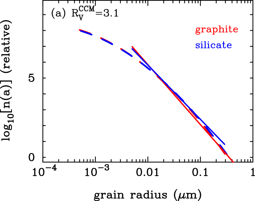
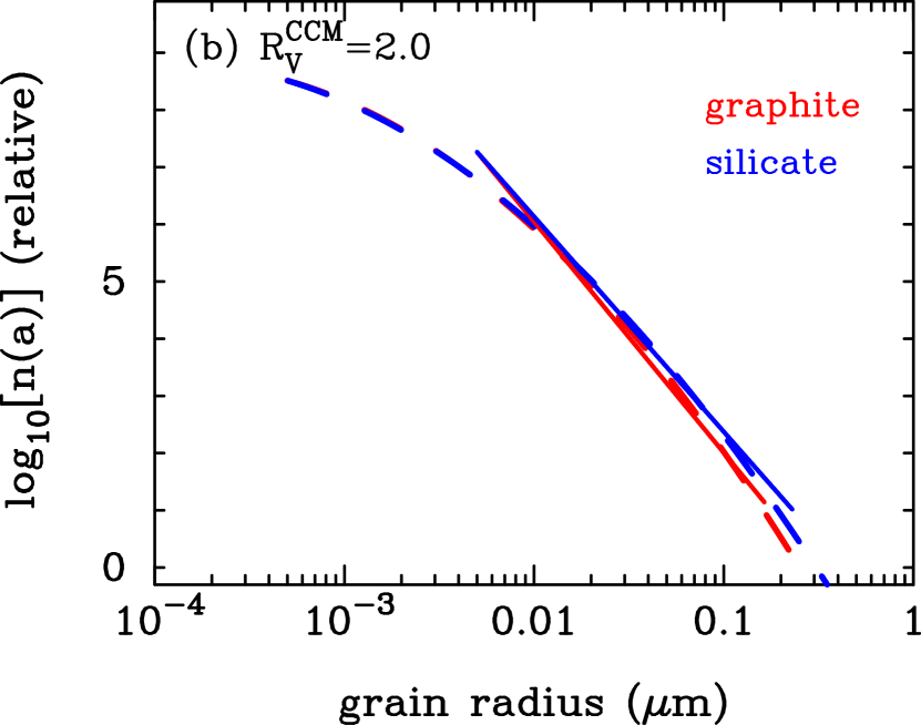
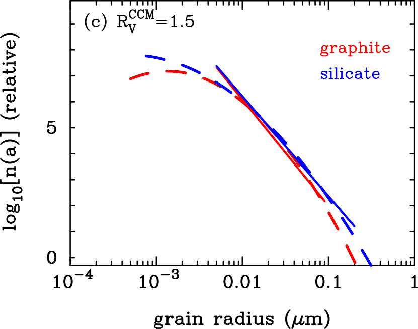
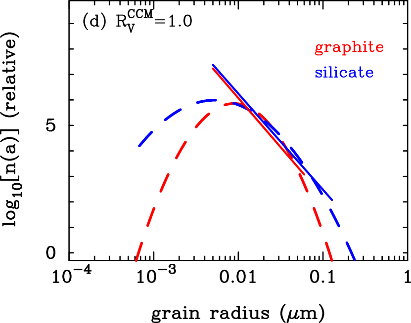
Figure 3: Grain size distributions that lead to the best-fit to the extinction curves with (a) $R_{V}^{\rm CCM}=3.1$ (b) $2.0$, (c) $1.5$, and (d) $1.0$. In each panel, the solid lines show the power-law size distributions obtained from Model 5, while the dashed lines indicate the results from lognormal size distributions from Model 5s. Graphite and silicate are drawn in red and blue, respectively.

Table 6: Average radii $\langle a_{{\rm ave},j}^{m}\rangle$ of graphite and silicate grains in units of $\mu$m for Models 1 and 5 in Table 2 and for Model 5s in Table 3.

Dust model		graphite			silicate
	$m=1$	$m=2$	$m=3$	$m=1$	$m=2$	$m=3$
$R_{V}^{\rm CCM}=3.1$
Model 1	0.0083	0.0103	0.0155	0.0083	0.0103	0.0155
Model 2	0.0082	0.0102	0.0152	0.0082	0.0102	0.0152
Model 4	0.0082	0.0100	0.0150	0.0082	0.0100	0.0150
Model 5	0.0078	0.0093	0.0139	0.0085	0.0109	0.0171
Model 5s	0.0022	0.0041	0.0087	0.0022	0.0043	0.0095
$R_{V}^{\rm CCM}=2.0$
Model 1	0.0083	0.0100	0.0138	0.0083	0.0100	0.0138
Model 2	0.0074	0.0085	0.0111	0.0074	0.0085	0.0111
Model 4	0.0077	0.0090	0.0119	0.0077	0.0090	0.0119
Model 5	0.0074	0.0084	0.0110	0.0078	0.0093	0.0129
Model 5s	0.0019	0.0031	0.0056	0.0020	0.0034	0.0066
$R_{V}^{\rm CCM}=1.5$
Model 1	0.0082	0.0098	0.0128	0.0082	0.0098	0.0128
Model 2	0.0071	0.0078	0.0094	0.0071	0.0078	0.0094
Model 4	0.0079	0.0093	0.0120	0.0079	0.0093	0.0120
Model 5	0.0074	0.0082	0.0099	0.0077	0.0090	0.0121
Model 5s	0.0042	0.0060	0.0087	0.0030	0.0049	0.0084
$R_{V}^{\rm CCM}=1.0$
Model 1	0.0081	0.0094	0.0114	0.0081	0.0094	0.114
Model 2	0.0066	0.0070	0.0077	0.0066	0.0070	0.0077
Model 4	0.0085	0.0100	0.0122	0.0085	0.0100	0.0122
Model 5	0.0076	0.0086	0.0102	0.0078	0.0091	0.0119
Model 5s	0.0129	0.0146	0.0166	0.0111	0.0143	0.0184

3.3 Allowed ranges of $a_{\rm max}$, $q$ and $f_{\rm gs}$ for power-law size distribution

In Section 3.1, we have shown that the CCM extinction curves with $R_{V}^{\rm CCM}=$ 1.0–3.1 can be reasonably fitted by the simplest power-law dust model with $q=3.5$ through taking an appropriate set of $a_{\rm max}$ and $f_{\rm gs}$. We found that, for Model 1, the optimum maximum cut-off radius $a_{\rm max}$ decreases from $a_{\rm max}=0.24$ $\mu$m for $R_{V}=3.1$ down to $a_{\rm max}=0.057$ $\mu$m for $R_{V}=1.0$, with a range of $f_{\rm gs}=$ 0.45–0.6. However, the best-fit value is not a unique solution; there should be other combinations of $a_{\rm max}$ and $f_{\rm gs}$ that still yield reasonable fits to the extinction data. Therefore, given that there are some uncertainties on the data of extinction curves, it should be inspected what extent of the change in $a_{\rm max}$ and $f_{\rm gs}$ is allowable.

In order to quantify the allowed ranges of $a_{\rm max}$ and $f_{\rm gs}$, we introduce the average extinction uncertainty $\tilde{\sigma}$, defined as $\tilde{\sigma}=\sum\sigma_{i}/N_{\rm data}$, where $\sigma_{i}$ are the uncertainties of extinction data at the reference wavelengths $\lambda_{i}$. Then, if the dispersion $\chi_{1}$ calculated for a given combination of $a_{\rm max}$ and $f_{\rm gs}$ is smaller than $\tilde{\sigma}$, we consider it as reproducing the extinction curves within the 1$\sigma$ errors. Using the values of $\sigma_{i}$ in Table 1 leads to the average uncertainty of $\tilde{\sigma}=0.115$. It should be kept in mind that some of $\sigma_{i}$ in Table 1 are inferred from those at the closest reference wavelengths, so the absolute value of $\tilde{\sigma}$ is quite arbitrary. Nevertheless, the introduction of such a criterion for the dispersion would give a meaningiful indication for the allowed range of $a_{\rm max}$ and $f_{\rm gs}$.

Figure 4 shows the contours within which the combinations of $a_{\rm max}$ and $f_{\rm gs}$ satisfy the 1$\sigma$ condition $\chi_{1}\leq\tilde{\sigma}$ for $R_{V}^{\rm CCM}=$ 3.1, 2.0, and 1.5. For $R_{V}^{\rm CCM}=1.0$, there is no combination of $a_{\rm max}$ and $f_{\rm gs}$ within the 1$\sigma$ error. Thus, we plot the 2$\sigma$ range (that is, combinations of $a_{\rm max}$ and $f_{\rm gs}$ with $\chi_{1}\leq 2\tilde{\sigma}$) for $R_{V}^{\rm CCM}=1.0$ (we also show the 2$\sigma$ contours for $R_{V}^{\rm CCM}=$ 2.0 and 1.5). We observe that, for each $R_{V}^{\rm CCM}$, a higher $f_{\rm gs}$ is needed for a lower $a_{\rm max}$ to produce fits within the 1$\sigma$ errors for $R_{V}^{\rm CCM}=$1.5–3.1. For $R_{V}^{\rm CCM}=3.1$, the 1$\sigma$ ranges of $a_{\rm max}$ and $f_{\rm gs}$ are 0.199 $\mu$m $\leq a_{\rm max}\leq$ 0.294 $\mu$m and 0.31 $\leq f_{\rm gs}\leq$ 1.07, whereas the allowed ranges of $a_{\rm max}$ lie just around its optimum values for $R_{V}^{\rm CCM}\leq 2.0$, keeping the trend that $a_{\rm max}$ decreases with decreasing $R_{V}^{\rm CCM}$. On the other hand, $f_{\rm gs}$ is relatively uniform with the values of $\simeq$0.4–0.6, regardless of $R_{V}^{\rm CCM}$. This means that the fraction of graphite mass of the total dust mass is in a narrow range of $f_{\rm gs}/(1+f_{\rm gs})\simeq$ 0.3–0.4.

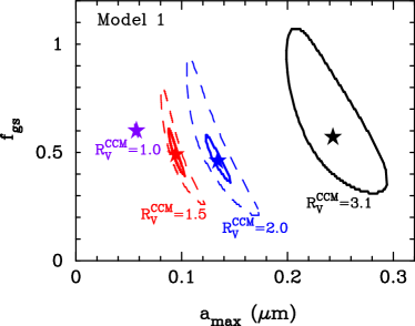
Figure 4: Contour plots showing the allowed regions of $a_{\rm max}$ and $f_{\rm gs}$ with which Model 1 can yield fits to the CCM extinction curves within the 1$\sigma$ errors (solid lines) for $R_{V}^{\rm CCM}=$ 1.5, 2.0, and 3.1. For $R_{V}^{\rm CCM}=$ 1.0, 1.5, and 2.0, the contours within the 2$\sigma$ errors are also drawn by the dashed lines. The best-fit combination of $a_{\rm max}$ and $f_{\rm gs}$ is marked by the filled star for each $R_{V}^{\rm CCM}$. Note that the size of 2$\sigma$ contour for $R_{V}^{\rm CCM}=$ 1.0 is comparable with that of the star symbol.

Next we consider the variation of the power-law index $q$. As demonstrated in Section 3.1, Model 2, in which $a_{\rm max}$ is fixed as 0.25 $\mu$m, cannot reproduce the CCM curves with $R_{V}^{\rm CCM}=$ 1.5, and 1.0; in these cases, the dispersion $\chi_{1}$ is larger than $2\tilde{\sigma}=0.23$ even for their best-fit combinations of $q$ and $f_{\rm gs}$ (see Table 4). This implies that the change in $a_{\rm max}$ must be essential for the reproduction of the steep extinction curves with $R_{V}^{\rm CCM}\leq 1.5$. Figure 5 presents the $1\sigma$ ($2\sigma$) ranges of combination of $a_{\rm max}$ and $q$ for $R_{V}^{\rm CCM}=$ 3.1, 2.0, and 1.5 ($R_{V}^{\rm CCM}=$ 1.0) under the assumption that graphite and silicate have the same size distribution (i.e., $a_{\rm max}=a_{\rm max,gra}=a_{\rm max,sil}$ and $q=q_{\rm gra}=q_{\rm sil}$ which corresponds to Model 4). The contours show that, for a given value of $R_{V}^{\rm CCM}$, a higher $q$ is needed for a higher $a_{\rm max}$. However, the power index does not increase with going from $R_{V}^{\rm CCM}=2.0$ down to 1.0; $q$ is confined within the range of $q=$ 3–4 for any value of $R_{V}^{\rm CCM}$ considered in this work, while there is a clear tendency that $a_{\rm max}$ decreases with decreasing $R_{V}^{\rm CCM}$. This indicates that the reduction in $a_{\rm max}$ is preferable to the enhancement in $q$ for describing the highly steep extinction curves. We also note that, for the cases of $R_{V}^{\rm CCM}=$ 2.0, 1.5, and 1.0, the best-fit combinations of $a_{\rm max}$ and $q$ in Model 4 lead to the similar average radii of $\langle a_{{\rm ave},j}^{3}\rangle\simeq 0.012$ $\mu$m. This is an additional indication that the average radius is not a good measure of size distributions that feature the extinction curves.

In summary, the variation of the extinction curves is mostly described by the change in $a_{\rm max}$ in the context of the power-law size distribution. For $R_{V}^{\rm CCM}=$ 1.0–3.1, the range of $q=$ 3–4 reasonably fits to the CCM curves. The mass ratio of graphite to silicate is constrained to be $0.4\leq f_{\rm gs}\leq 0.6$, which interestingly well agrees with the range $0.3\leq f_{\rm gs}\leq 0.7$ estimated from the analysis of the average extinction curve and abundance constraints in the MW (Nozawa & Fukugita, 2013). This suggests that the composition of dust toward lines of sight with $R_{V}^{\rm CCM}\leq 2.0$ would not be largely different from that in the MW.

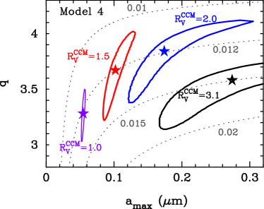
Figure 5: Contour plots showing the allowed regions of $a_{\rm max}$ and $q$ with which Model 4 can yield fits to the CCM extinction curves within the 1$\sigma$ errors for $R_{V}^{\rm CCM}=$ 1.5, 2.0, and 3.1 (thick solid lines). For $R_{V}^{\rm CCM}=$ 1.0, the contour within the 2$\sigma$ errors is drawn by thin solid line. The best-fit combination of $a_{\rm max}$ and $q$ is marked by the filled star for each $R_{V}^{\rm CCM}$. The dotted curves indicate the trajectories of specific average radii $\langle a_{{\rm ave}j}^{3}\rangle$ calculated from Equation (8) adopting $m=3$: $\langle a_{{\rm ave}j}^{3}\rangle=$ 0.01, 0.012, 0.015, and 0.02 $\mu$m from top to bottom.

4 Discussions

4.1 Dependence of $R_{V}$ on $a_{\rm max}$

We have demonstrated that the two-component model of graphite and silicate with power-law size distributions is a competent dust model that can explain the systematic behaviors of extinction curves for a wide variety of $R_{V}^{\rm CCM}$. However, the $R_{V}^{\rm mod}$ calculated from our dust models does not match the $R_{V}^{\rm CCM}$ that is referred to in deriving the data of the extinction curve; for all the power-law dust models considered in this study, $R_{V}^{\rm mod}$ is higher than $R_{V}^{\rm CCM}$ as seen from Table 4. This indicates that our dust model can account for the overall shape of extinction curves but cannot accurately reproduce the extinction ratio between specific wavelengths.

Figure 6 depicts the $R_{V}^{\rm mod}$ calculated from Model 1 as a function of $a_{\rm max}$ for $f_{\rm gs}=$ 0.4, 0.6, and 1.0. We can see that the dependence of $R_{V}^{\rm mod}$ on $f_{\rm gs}$ is weak, although there appears slight difference at $a_{\rm max}=$ 0.1–0.4 $\mu$m. More importantly, as $a_{\rm max}$ increases, $R_{V}^{\rm mod}$ decreases at $a_{\rm max}\leq 0.06$ $\mu$m and increases at $a_{\rm max}\geq 0.07$ $\mu$m, having the minimum value of $R_{V}^{\rm mod}\simeq 1.46$ at $a_{\rm max}\simeq 0.065$ $\mu$m for any value of $f_{\rm gs}$. We have confirmed that this dependence of $R_{V}^{\rm mod}$ on $a_{\rm max}$ is not sensititve to the minimum cut-off radius $a_{\rm min}$ as long as $a_{\rm min}\leq 0.01$ $\mu$m. Thus, if the measured values of $R_{V}<1.4$ are real, they could not be interpreted by the simple dust model considered here. The unfeasibility of such low $R_{V}$, as well as the descrepancy between $R_{V}^{\rm mod}$ and $R_{V}^{\rm CCM}$, implies that more sophisticated dust models which adopt more fine-tuned size distribution function and involve additional components other than graphite and silicate are necessary for consistently explaining the shape of extinction curve and the value of $R_{V}$.

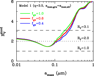
Figure 6: Dependence of $R_{V}^{\rm mod}$ on $a_{\rm max}$ calculated from Model 1 with $q=3.5$ and $a_{\rm max}=a_{\rm max,gra}=a_{\rm max,sil}$ for $f_{\rm gs}=$ 0.4, 0.6, and 1.0. The minimum cut-off radii are fixed to $a_{\rm min}=$ 0.005 $\mu$m. The two dashed horizontal lines represent $R_{V}=$ 3.1 and 1.0, and the dotted line exhibits $R_{V}=$ 2.0.

We also note that the measured value of $R_{V}$ is unlikely to be a good probe for constraining the properties of interstellar dust. For example, as seen in Figure 6, there are two possible values of $a_{\rm max}$ ($a_{\rm max}\simeq$ 0.026 $\mu$m and 0.11 $\mu$m) that realize $R_{V}=2.0$. This suggests that the properties of dust cannot be necessarily determined uniquely only from $R_{V}$ being the ratio of extinction in $V$ and $B$ bands, unless $R_{V}$ is an extremely low or high value. In order to extract the information on the properties of interstellar dust, the extinction data over a broad range of wavelengths are essential, which is demonstrated in more details in the next subsection.

4.2 Necessity of UV extinction data

So far, we have performed the fitting to the extinction data at all the reference wavelengths covering UV to near-infrared. However, the data at UV wavelengths cannot be always acquired, and in most cases, we have to derive the extinction law by relying only on the data at optical to near-infrared wavelengths. In addition, the extinction curves in external galaxies such as Large and Small Magellanic Clouds do not show a remarkable 2175 Å bump (Gordon et al., 2003) and cannot be described as the CCM curves. Thus, it would be interesting to see how the results of fitting can be changed in the cases that the UV extinction data are not taken into account, especially in the absence of data around the 2175 Å bump.

Table 7: A set of the best-fit parameters obtained for some dust models that do not consider the UV extinction data.

Dust model$\,{}^{a}$	$q_{\rm gra}$	$a_{\rm max,gra}$	$q_{\rm sil}$	$a_{\rm max,sil}$	$f_{\rm gs}$	$\chi_{1}$	$R_{V}^{\rm cal}$
		($\mu$m)		($\mu$m)
$R_{V}^{\rm CCM}=3.1$
Model 1nb	3.50	0.259	3.50	0.259	0.50	0.0224	3.41
Model 1nu	3.50	0.266	3.50	0.266	0.41	0.0234	3.42
$R_{V}^{\rm CCM}=2.0$
Model 1nb	3.50	0.128	3.50	0.128	0.50	0.0605	2.12
Model 5nb	1.50	0.0729	3.94	0.441	0.18	0.0286	2.11
Model 1nu	3.50	0.201	3.50	0.201	0.16	0.0354	2.30
$R_{V}^{\rm CCM}=1.5$
Model 1nb	3.50	0.0896	3.50	0.0896	0.55	0.0553	1.68
Model 5nb	2.00	0.0741	2.31	0.0358	0.63	0.0322	1.53
Model 1nu	3.50	0.0830	3.50	0.0830	4.00	0.0458	1.65
$R_{V}^{\rm CCM}=1.0$
Model 1nb	3.50	0.0618	3.50	0.0618	0.53	0.215	1.46
Model 1nu	3.50	0.149	3.50	0.149	0.00	0.115	1.18

^aModel 1nb and Model 1nu are the same as Model 1 in Table 2 but do not take into account, respectively, the five data around the 2175 Å bump at $1/\lambda=$ 3.0–5.2 $\mu$m^-1 and the seven UV data at $1/\lambda<$ 3.0 $\mu$m^-1 for the fitting calculations. Model 5nb is the same dust model as Model 5 in Table 2 but does not take the data around the UV bump in consideration.

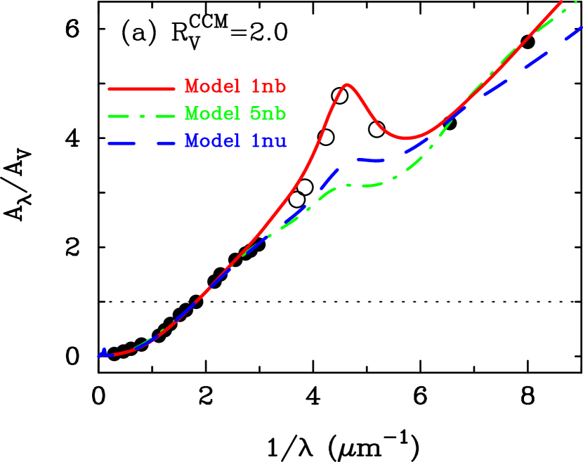
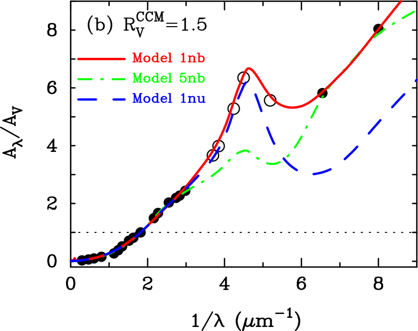
Figure 7: Extinction curves for (a) $R_{V}^{\rm CCM}=2.0$ and (b) $R_{V}^{\rm CCM}=1.5$, calculated from the best-fit combonations of $a_{\rm max}$ and $f_{\rm gs}$ for Model 1nb (solid) and Model 1nu (dashed) with $q=3.5$ and $a_{\rm max,gra}=a_{\rm max,sil}$. Model 1nb performs the fitting to the data of the extinction curves in which the five data around the UV bump at $1/\lambda=$ 3.0–5.2 $\mu$m^-1 are excluded, while Model 1nu does not include the UV data at $1/\lambda<$ 3.0 $\mu$m^-1 for the fitting calculations. The dot-dashed line depicts the extinction curves from Model 5nb, which uses the same extinction data as Model 1nb but parameterizes all of the five quantities relevant to the power-law distribution. The circles are the extinction data at the reference wavelengths, derived from the CCM formula for each $R_{V}^{\rm CCM}$ value, where the open symbols signify the data disregarded for Model 1nb and Model 5nb.

From this motivation, we do the fitting calculations for the data sets that do not include the wavelengths ($1/\lambda=$ 3.0–5.2 $\mu$m^-1) around the 2175 Å bump (but still include the two far-UV wavelengths at $1/\lambda=$ 6.5 and 8.0 $\mu$m^-1). For purposes of illustration, we here focus on the dust models with power-law size distributions. As been done before, we evaluate the goodness of fitting with Equation (7), for which $N_{\rm data}=17$ with the five data around the UV bump being excluded.

Table 7 presents the best-fit parameters obtained from the fitting calculations that do not take account of the data around the UV bump for some dust models considered in this study. The corresponding extinction curves are shown in Figure 7(a) and 7(b) for $R_{V}^{\rm CCM}=2.0$ and 1.5, respectively. We can see that, when we assume $q=3.5$ and $a_{\rm max,gra}=a_{\rm max,sil}$ (referred to as Model 1nb), the best-fit combinations of $a_{\rm max}$ and $f_{\rm gs}$, even if the UV-bump data are not considered, are chosen so that the resulting extinction curves have a prominent 2175 Å bump like those from Model 1, which do not neglect the UV-bump data. This seems that the data near 2175 Å may be insignificant in extracting the properties of dust from the measured extinction curves. However, this is not true; when we parameterize all of the five quantities ($q_{\rm gra}$, $a_{\rm max,gra}$, $q_{\rm sil}$, $a_{\rm max,sil}$, and $f_{\rm gs}$) relevant to the power-law size distribution (referred to as Model 5nb), the best-fit models yield a much weaker 2175 Å bump for both $R_{V}^{\rm CCM}=2.0$ and 1.5. In particular, the result without the UV-bump data for $R_{V}^{\rm CCM}=2.0$ prefers a highly silicate-dominated dust composition ($f_{\rm gs}=0.18$, compared to the nominal range of $f_{\rm gs}=$ 0.4–0.6), indicating that the data around the 2175 Å bump are essential for determining the mass fraction of graphite.

In addition, if we do not include the data at UV wavelengths shorter than 0.3 $\mu$m, distinct extinction curves appear even in the case of $q=3.5$ and $a_{\rm max,gra}=a_{\rm max,sil}$ (referred to as Model 1nu for which $N_{\rm data}=15$ without the seven data in UV regions). As seen from Figure 7, the extinction curves from Model 1nu for $R_{V}^{\rm CCM}=$ 2.0 and 1.5 well reproduce the extinction data at $1/\lambda\leq$ 3.0 $\mu$m^-1. However, at $1/\lambda\geq 3.0$ $\mu$m^-1, these extinction curves do not resemble to their corresponding ones from Model 1; the UV extinction curve for $R_{V}^{\rm CCM}=$ 2.0 shows a less prominent 2175 Å bump because of a smaller abundance of graphite ($f_{\rm gs}=0.16$), whereas the best fit for $R_{V}^{\rm CCM}=$ 1.5 requires a very high abundance of graphite ($f_{\rm gs}\geq 4.0$), resulting in an extremely conspicuous UV bump.

These analyses clearly demonstrate that, despite using the same extinction data at optical to near-infrared wavelengths, the different results come out depending on whether the UV extinction data are taken into account or not. Therefore, we conclude that the extinction data at UV wavelengths are crucial for reliablely assessing the composition and size distribution of interstellar dust from the measured extinction curves.

5 Conclusion

We have investigated the properties of interstellar dust responsible for the peculiar extinction laws with $R_{V}=$ 1.0–2.0 measured toward Type Ia supernovae (SNe Ia). We perform the fitting calculations to the measured extinction curves, for which we adopt the extinction values at the reference wavelengths derived with the empirical one-parameter formula by Cardelli et al. (1989). As a dust model for calculating the extinction curves, we consider a two-component model composed of graphite and silicate with power-law and lognormal size distributions.

We first confirm that our dust model can reproduce the extinction curves with $R_{V}^{\rm CCM}=3.1$ that is taken to be a typical value in the Milky Way (MW). Then, we find that even the simplest dust model with the power index of $q=3.5$ can account for the entire shapes of steep extinction curves described by $R_{V}^{\rm CCM}=2.0$, $1.5$, and $1.0$ with appropriate combinations of the maximum cut-off radius $a_{\rm max}$ and mass ratio of graphite to silicate $f_{\rm gs}$. In particular, $a_{\rm max}$ is found to be an important quantity to describe the variety of extinction curves, and decreases from $\simeq$0.24 $\mu$m for $R_{V}^{\rm CCM}=3.1$ down to $\simeq$0.06 $\mu$m for $R_{V}^{\rm CCM}=1.0$. On the other hand, $f_{\rm gs}$ takes a relatively narrow range of $\simeq$0.4–0.6, indicating the mass ratio of graphite to silicate is not changed dramatically for different $R_{V}^{\rm CCM}$.

We have demonstrated that the lognormal grain size distribution can also work well in reproducing the CCM curves with $R_{V}^{\rm CCM}=$ 1.0–3.1 by taking the very small characteristic radius $a_{0,j}$ and relatively large standard deviation $\gamma_{j}$ of the distribution. Furthermore, from the comparison of the average grain radii between the best-fit power-law and lognormal size distributions, we suggest that the average radius is not a proper quantity as representing the properties of dust that explains the extinction curves. Finally, we point out that the extinction data at a limited range of wavelengths, such as a single value of $R_{V}$, do not allow us to uniquely determine the properties of dust, and that the extinction data over a wide range of wavelengths including the UV data are essential for constraining the composition and size distribution of interstellar dust.

Our main conclusion is that, in order to explain the steep extinction curves suggested for SNe Ia, the size distribution of interstellar dust in their host galaxies is biased to small sizes, compared to that in the MW. Since SNe Ia are known to happen in any types of galaxies, this implies that large grains ($a\geq$ $\sim$ 0.1 $\mu$m) are lacking in galaxies other than the MW. Why are the sizes of interstellar dust so small in external galaxies? This may presuppose that the evolution history of the MW is somehow different from the other galaxies so that the interstellar dust in the MW has the exceptional properties. There is also a possibility that the measured extinction curves do not reflect pure extinction but are distorted by other effects such as contamination of scattered lights at shorter wavelengths. Nagao et al. (2016) showed that small silicate grains and/or polycyclic aromatic hydrocarbons (PAHs) are needed for producing a low $R_{V}$ through multiple scattering. Hence, this possibility may require that the host galaxies of SNe Ia contain abundant small silicate grains and PAHs. Another possibility is that something is amiss in the process of extracting the extinction curves from the observations of SNe Ia. Given that SNe Ia are ideal objects to measure the extinction curves in external galaxies, these subjects should be addressed from both observational and theoretical points of view.

References

- Amanullah et al. (2014) Amanullah, R., et al., 2014, The peculiar extinction law of SN 2014J measured with the Hubble Space Telescope, Astrophys. J., 788, L21 (6pp).
- Amanullah & Goobar (2011) Amanullah, R., Goobar, A., 2011, Perturbations of SNe Ia light curves, colors, and spectral features by circumstellar dust, Astrophys. J., 735, 20 (10pp).
- Asano et al. (2013) Asano, R. S., Takeuchim T. T., Hirashita, H., Nozawa, T., 2013, What determines the grain size distribution in galaxies? Mon. Not. R. Astron. Soc., 432, 637–652.
- Biermann & Harwit (1980) Biermann, P., Harwit, M., 1980, On the origin of the grain-size spectrum of interstellar dust, Astrophys. J., 241, L105–L107.
- Brown et al. (2015) Brown, P. J., et al., 2015, SWIFT ultraviolet observations of supernova 2014J in M82: large extinction from interstellar dust, Astrophys. J., 805, 74 (13pp).
- Cardelli et al. (1989) Cardelli, J. A., Clayton, G. C., Mathis, J. S., 1989, The relationship between infrared, optical, and ultraviolet extinction, Astrophys. J., 345, 245–256.
- Clayton et al. (2003) Clayton, G. C., Wolff, M. J., Sofia, U., Gordon, K. D., Misselt, K. A., 2003, Dust grain size distributions from MRN to MEM, Astrophys. J., 588, 871–880.
- Conley et al. (2007) Conley, A., Carlberg, R. G., Guv, J., Howell, D. A., Jha, S., Ruess, A. G., Sullivan, M., Is there evidence for a Hubble bubble? The nature of Type Ia supernova colors and dust in external galaxies, Astrophys. J., 664, L13–L16.
- Dalcanton et al. (2009) Dalcanton, J. J., et al., 2009, The ACS nearby galaxies survey treasury, Astrophys. J. Suppl., 183, 67–108.
- Doi et al. (2010) Doi, M., et al., 2010, Photometric response functions of the Sloan Digital Sky Survey imager, Astronom. J., 139, 1628–1648.
- Draine (2003) Draine, B. T., 2003, Scattering by interstellar dust grains. II. X-ray, Astrophys. J., 598, 1026–1037.
- Draine & Lee (1984) Draine, B. T., Lee, H. M., 1984, Optical properties of interstellar graphite and silicate grains, Astrophys. J., 285, 89–108.
- Draine & Malhotra (1993) Draine, B. T., Malhotra, S., 1993, On graphite and the 2175 Å extinction profile, Astrophys. J., 414, 632–645.
- Dressel (2016) Dressel, L., 2016, Wide Field Camera 3 Instrument Handbook, Version 8.0, (Baltimore: STScI).
- Folatelli et al. (2010) Folatelli, G., et al., 2010, The Carnegie supernova project: Analysis of the first sample of low-redshift Type-Ia supernovae, Astronom. J., 139, 120–144.
- Foley et al. (2014) Foley, R. J. , et al., 2014, Extensive HST ultraviolet spectra and multiwavelength observations of SN 2014J in M82 indicate reddening and circumstellar scattering by typical dust, Type-Ia supernovae, Mon. Not. R. Astron. Soc., 443, 2887–2906.
- Gao et al. (2015) Gao, J., Jiang, B. W., Li, A., Li, J., Wang, X., 2015, Physical dust models for the extinction toward supernova 2014J in M82, Astrophys. J., 807, L26 (6pp).
- Goobar (2008) Goobar, A., 2008, Low from circumstellar dust around supernovae, Astrophys. J., 686, L103–L106.
- Goobar et al. (2014) Goobar, A., et al., 2014, The rise of SN 2014J in the nearby galaxy M82, Astrophys. J., 784, L12 (6pp).
- Gordon et al. (2003) Gordon, K. D., Clayton, G. C., Misselt, K. A., Landolt, A. U., Wolff, M. J., 2003, A quantitative comparison of the Small Magellanic Cloud, Large Magellanic Cloud, and Milky Way ultraviolet to near-infrared extinction curves, Astrophys. J., 594, 279–293.
- Hirashita et al. (2008) Hirashita, H., Nozawa, T., Takeuchi, T. T., Kozasa, T., 2008, Extinction curves flattened by reverse shocks in supernovae, Mon. Not. R. Astron. Soc., 384, 1725–1732.
- Hirashita & Nozawa (2013) Hirashita, H., Nozawa, T., 2013, Synthesized grain size distribution in the interstellar medium, Earth, Planets, and Space, 65, 183–192.
- Hirashita et al. (2015) Hirashita, H., Nozawa, T., Villaume, A., Srinivasan, S., 2015, Dust processing in elliptical galaxies, Mon. Not. R. Astron. Soc., 454, 1620–1633.
- Hoang (2015) Hoang, T., 2015, Properties and alignment of interstellar dust grains toward Type Ia supernovae with anomalous polarization curves, Mon. Not. R. Astron. Soc., submitted, arXiv:1510.01822.
- Howell (2011) Howell, D. A., 2011, Type Ia supernovae as stellar endpoints and cosmological tools, Nat. Commun., 2, 350 (10pp).
- Johansson et al. (2013) Johansson, J., Amanullah, R., Goobar, A., 2013, Herschel limits on far-infrared emission from circumstellar dust around three nearby Type Ia supernovae, Mon. Not. R. Astron. Soc., 431, L43–L47.
- Johansson et al. (2014) Johansson, J., et al., 2014, Spitzer observations of SN 2014J and properties of mid-IR emission in Type Ia supernovae, Mon. Not. R. Astron. Soc., submitted, arXiv:1411.3332.
- Jones et al. (2013) Jones, A. P., Fanciullo, L., Köhler, M., Verstraete, L., Guillet, V., Bocchio, M., Ysard, N., The evolution of amorphous hydrocarbons in the ISM: dust modelling from a new vantage point, Astronom. Astrophys. J., 558, A62 (22pp).
- Kawabata et al. (2014) Kawabata, K. S., et al., 2014, Optical and near-infrared polarimetry of highly reddened Type Ia supernovae 2014J: peculiar properties of dust in M82, Astrophys. J., 795, L4 (5pp).
- Lampeitl et al. (2010) Lampeitl, H., et al., 2010, The effect of host galaxies on Type Ia supernovae in the SDSS-II supernova survey, Astrophys. J., 722, 566–576.
- Maeda et al. (2015) Maeda, K., Nozawa, T., Nagao, T., Motohara, K., 2015, Constraining the amount of circumstellar matter and dust around Type Ia supernovae through near-infrared echoes, Mon. Not. R. Astron. Soc., 452, 3281–3292.
- Marion et al. (2015) Marion, G. H., et al., 2015, Early observations and analysis of the Type Ia SN 2014J in M82, Astrophys. J., 798, 39 (12pp).
- Mathis et al. (1977) Mathis, J. S., Rumpl, W., Nordsieck, K. H., 1977, The size distribution of interstellar grains, Astrophys. J., 217, 425–433.
- Morrissey et al. (2005) Morrissey, P., et al., 2005, The on-orbit performance of the Galaxy Evolution Explorer, Astrophys. J., 619, L7–L10.
- Nagao et al. (2016) Nagao, T., Maeda, K., Nozawa, T., 2016, Extinction laws toward stellar sources within a dusty circumstellar medium and implications for Type Ia supernovae, Astrophys. J., 823, 104 (10pp).
- Nordin et al. (2008) Nordin, J., Goobar, A., Jakob, J., 2008, Quantifying systematic uncertainties in supernova cosmology, Journal of Cosmology and Astroparticle Phys., 02, 008 (21pp).
- Nozawa & Fukugita (2013) Nozawa, T., Fukugita, M., 2013, Properties of dust grains probed with extinction curves, Astrophys. J., 770, 27 (13pp).
- Nozawa et al. (2007) Nozawa, T., Kozasa, T., Habe, A., Dwek, E., Umeda, H., Tominaga, N., Maeda, K., Nomoto, K., 2007, Evolution of dust in primordial supernova remnants: can dust grains formed in the ejecta survive and be injected into the early interstellar medium? Astrophys. J., 666, 955–966.
- Patet et al. (2015) Patat, F., et al., 2015 Properties of extragalactic dust inferred from linear polarimetry of Type Ia supernovae, Astron. Astrophys. J., 577, A53 (10pp).
- Poole et al. (2008) Poole, T. S., et al., 2008, Photometric calibration of the Swift ultraviolet/optical telescope, Mon. Not. R. Astron. Soc., 383, 627–645.
- Skrutskie et al. (2006) Skrutskie, M. F., et al., 2006, The two micron all sky survey (2MASS), Astronom. J., 131, 1163–1183.
- Sullivan (2010) Sullivan, M., et al., 2010, The dependence of Type Ia supernovae luminosities on their host galaxies, Mon. Not. R. Astron. Soc., 406, 782–802.
- Telesco et al. (2015) Telesco, C. M., et al., 2015 Mid-IR spectra of Type Ia SN 2014J in M82 spanning the first 4 months, Astrophys. J., 798, 93 (9pp).
- Wang (2005) Wang, L., 2005, Dust around Type Ia supernovae, Astrophys. J., 635, L33–L36.
- Weingartner & Draine (2001) Weingartner, J. C., Draine, B. T., 2001, Dust grain-size distributions and extinction in the Milky Way, Large Magellanic Cloud, and Small Magellanic Cloud, Astrophys. J., 548, 296–309.
- Yasuda & Kozasa (2012) Yasuda, Y., Kozasa, T., 2012, Formation of SiC grains in pulsation-enhanced dust-driven wind around carbon-rich asymptotic giant branch stars, Astrophys. J., 745, 159 (14pp).
- Zubko et al. (2004) Zubko, V., Dwek, E., Arendt, R. G., 2004, Interstellar dust models consistent with extinction, emission, and abundance constraints, Astrophys. J. Suppl., 152, 211–249.