Emergence of low noise frustrated states in E/I balanced neural networks

Abstract

We study emerging phenomena in binary neural networks where, with a probability $c$ synaptic intensities are chosen according with a Hebbian prescription, and with probability $(1-c)$ there is an extra random contribution to synaptic weights. This new term, randomly taken from a Gaussian bimodal distribution, balances the synaptic population in the network so that one has $80\%-20\%$ relation in E/I population ratio, mimicking the balance observed in mammals cortex. For some regions of the relevant parameters, our system depicts standard memory (at low temperature) and non-memory attractors (at high temperature). However, as $c$ decreases and the level of the underlying noise also decreases below a certain temperature $T_{t}$, a kind of memory-frustrated state, which resembles spin-glass behavior, sharply emerges. Contrary to what occurs in Hopfield-like neural networks, the frustrated state appears here even in the limit of the loading parameter $\alpha\rightarrow 0$. Moreover, we observed that the frustrated state in fact corresponds to two states of non-vanishing activity uncorrelated with stored memories, associated, respectively, to a high activity or Up state and to a low activity or Down state. Using a linear stability analysis, we found regions in the space of relevant parameters for locally stable steady states and demonstrated that frustrated states coexist with memory attractors below $T_{t}$. Then, multistability between memory and frustrated states is present for relatively small $c,$ and metastability of memory attractors can emerge as $c$ decreases even more. We studied our system using standard mean-field techniques and with Monte Carlo simulations, obtaining a perfect agreement between theory and simulations. Our study can be useful to explain the role of synapse heterogeneity on the emergence of stable Up and Down states not associated to memory attractors, and to explore the conditions to induce transitions among them, as in sleep-wake transitions.

Keywords: Balanced neural networks, frustrated activity states, Up/Down neural states

Department of Electromagnetism and Physics of the Matter and Institute “Carlos I” for Theoretical and Computational Physics, University of Granada, Granada, Spain, E-18071.

1 Introduction

Traditional Hopfield-like networks [1], which assume a Hebbian learning rule [2, 3] for synaptic intensities, have been widely tested to be convenient for recall of learned memories. In these networks, one can train the system to learn some predefined patterns of neural activity (e. g., related with some sensory information) through their storage at the synaptic intensities. After the learning process, and due to the synaptic modification it implies, each neuron in the network can be more or less excitable according with the strength of the synaptic intensities it receives. In this way, a Hopfield-like network is able to retrieve one of these stored patterns if the network receives an input similar to it by means the associative memory mechanism. Under a mathematical point of view, this recall of learned patterns occurs since synaptic modifications during learning make the stored patterns to become attractors of the underlying dynamics of the system [4, 5]. Then, if the input pattern puts the network activity within the basin of attraction of a given memory, the system can retrieve it.

The brain of mammals is able to recognize visual information or other sensory patterns by means of this associative memory mechanism [6, 7]. When information received through the senses reaches the brain sensory areas, neurons become firing or silent according to some information coding scheme [8]. It is well established, that this information activates these neuronal areas in such a way that when an excitatory neuron fires it induces the firing of neighboring neurons. To achieve this, some modifications on the synaptic weights has to be done any time neighboring neurons are active or inactive during the processing of sensory information [9, 10]. One of the most common used paradigms for learning is the so called Hebbian learning rule [2], which is often summarized as "Cells that fire together, wire together". Attending to this rule, the group of neurons related, for instance, to the green color and those to the smell of the field grass would fire together, and their connections would become stronger so that both feelings will activate correlated areas inside our brains [11]. Hebbian learning paradigm has been widely described to be present in different biological systems including brain mammals as in the traditional experiments of long-term potentation (LTP) [12] but also in invertebrates as in the honeybee antennal lobe [13] (where it serves as an olfactory sensory memory). Those two pieces of the same puzzle, namely a Hopfield like network – which provides the structure and the dynamic of a neural network – and Hebbian learning that is responsible of creating the optimal synaptic weights in order to retrieve predefined stored patterns of activity, works properly and they constitute the basics elements when trying to model and simulate auto-associative tasks in the brain.

On the other hand, it has been long observed that in mammals cortex there exists a balance between excitatory and inhibitory neurons [14, 15, 16] which seems important to regulate the activity in actual neural systems [17]. Traditionally Hopfield-like models do not account properly for this balance (although, as it is shown below, the Hebbian learning rule implies for random patterns the same amount of excitation and inhibition in these networks). In this work, we analyzed the implications that result from including a biophysically motivated balance of excitation and inhibition in autoassociative neural networks. We introduced this balance by adding a new random term with probability $(1-c)$ to Hebbian synaptic intensities – which occurs then with probability $c$ – drawn from a bimodal distribution. In order to mimic the experimental findings, the excitatory mode in this distribution has a probability which is four times larger than the inhibitory one but where its strength is four times lower. The resulting synaptic intensities satisfy the excitation/inhibition balance found in actual neural systems, and due to the presence of the Hebbian term with probability $c$, the model preserves the associative memory property for some regions of the relevant parameters.

Additionally, our system presents new intriguing features at low temperatures, even in the limit of the loading parameter $\alpha=\lim_{N\rightarrow\infty}P/N\rightarrow 0,$ with $P$ and $N$ being, respectively, the number of stored patterns and the network size. This includes the appearance at low temperatures of new type of stable sates where the associative memory property is lost, and which are embedded among the (also stable) traditional memory states. This multistable phase is such that the low-noise non-memory or frustrated states have largest basin of attractions than the traditional memory attractors. Moreover, for values of $c$ below some given value, the memory attractors become metastable so the frustrated states turn into the global attractor of the dynamics of the system. Besides, the frustrated attractors are not correlated with memory ones and are characterized by other type of order so that, depending on initial conditions, these states can correspond to a high activity or Up state, or to a low activity or Down state. Moreover, these frustrated states can not be the same as the traditional spin-glass states appearing in the Hopfield model at low temperature, since in this last case these type of states appear only for $\alpha>0.$

Future extension of our study here could be useful to understand how synapse heterogeneity can lead to the appearance, for instance, of Up/Down states in the mammalian cortex not correlated with memory attractors, and to explore the appearance of transitions among these states – as those observed during the sleep-wake transitions or anesthesia [18] – when some attractor destabilizing mechanisms, as for instance dynamic synapses [19, 20, 21] or hyperpolarizing potassium slow currents [22], are incorporated in the neural network model.

2 Models and Methods

Our starting point is a network of $N$ binary neurons whose possible states $s_{i}=0,1;\,\forall i=1,\ldots,N$ represent neurons in a silent or firing state, respectively. We then define a state evolution for the network, where each neuron obeys the following probabilistic, parallel and synchronous dynamics [5]:

$$P[s_{i}(t+1)=1]=\frac{1}{2}\left\{1+\tanh\left[2\beta\left(h_{i}(\mathbf{s},t)-\theta_{i}\right)\right]\right\}\quad\forall i=1,\ldots,N,$$ (1)

where $h_{i}(\mathbf{s},t)$ is the local field or the total input synaptic current arriving to neuron $i$, and which is defined as

$$h_{i}(\mathbf{s\mathrm{,t}})=\sum_{j\neq i}\omega_{ij}s_{j}(t)\varepsilon_{ij}.$$ (2)

Here $\varepsilon_{ij}$ is the connectivity matrix, that for simplicity we shall assume here to be that of a fully connected network, i.e. $\varepsilon_{ij}=1\forall i\neq j$ and $\epsilon_{ii}=0$ to avoid self-connections. The variable $s_{j}(t)$ represents the current sate of the $j^{th}$ presynaptic neuron and $\omega_{ij}$ is the matrix of synaptic weights where each element specifies the strength of the connection between the $i^{th}$ and $j^{th}$neurons. We denote also $\beta\equiv T^{-1}$ as the inverse of a temperature parameter $T$ – controlling the level of thermal noise in the system – such that $\beta\rightarrow\infty$ ($T=0$) implies a deterministic dynamics whereas for $\beta=0$ ($T\rightarrow\infty$) the network evolves fully randomly.

In our model, we assume that synaptic intensities or weights are given as

$$\omega_{ij}=c\omega_{ij}^{H}+\left(1-c\right)\omega_{ij}^{B}$$ (3)

$$\omega_{ii}=0$$

with $0\leq c\leq 1,$ and where we avoid self connections. The first term of the right-hand side of (3) refers to synaptic modifications due to learning. We assume that this term is given by the standard Hebbian learning rule that memorizes $P$ prescribed patterns of neural activity in the form [23, 4]

$$\omega_{ij}^{H}=\frac{1}{a(1-a)N}\sum_{\mu}\left(\xi_{i}^{\mu}-a\right)\left(\xi_{j}^{\mu}-a\right).$$ (4)

Here, $\left\{\xi_{i}^{\mu}=0,1\,;\,i=1,\ldots,N\right\}$ represents the $P$ stored random patterns with probability distribution [23, 4]

$$p\left(\xi_{i}^{\mu}\right)=a\delta\left(\xi_{i}^{\mu}-1\right)+\left(1-a\right)\delta\left(\xi_{i}^{\mu}\right)$$ (5)

where $a=\left\langle\xi_{i}^{\mu}\right\rangle$ is the mean level of neural activity in the pattern and $\delta(x)$ is the Dirac delta function. On the other hand, $\omega_{ij}^{B}$ in (3) accounts for a random contribution to the synaptic weights not directly associated to learning, as for instance synaptogenesis, synapse remodeling and homeostatic synaptic plasticity during life brain development [24], synaptic pruning during early stages of brain development [25, 26, 27], etc. Here, we consider $\omega_{ij}^{B}$ to be a random number drawn from the Gaussian bimodal distribution

$$p\left(\omega_{ij}^{B}\right)=\eta\mathcal{N}\left(\kappa\alpha,\sigma^{2}\right)+\left(1-\eta\right)\mathcal{N}\left(-4\kappa\alpha,\sigma^{2}\right)$$ (6)

with a main synaptic mode being excitatory (positive) and the other inhibitory (negative), where $0\leq\eta\leq 1$ is a parameter controlling the probability of each synaptic mode, and $\sigma^{2}$ is the variance of each distribution mode. Note that in this way $\omega_{ij}^{B}$ and $\omega_{ji}^{B}$ are random numbers not necessary equal but following the same distribution. Also in (6) $\alpha\equiv P/N$ is the loading parameter that measures the amount of patterns stored in the network relative to its size, and $\kappa>0$ is a arbitrary constant that controls the synaptic strength separation between the two modes. For a large number $P$ of independent unbiased random patterns and due to the “Central Limit Theorem”, the Hebbian variable $\omega_{ij}^{H}$ becomes approximatively Gaussian [28]. Moreover it can be analytically proof that with the choice (6) the model reproduces a balance between excitatory synapses $\left(\omega_{ij}>0\right)$ and inhibitory synapses $\left(\omega_{ij}<0\right)$ in the network, and that the strength of inhibitory synapses is four times the strength of the excitatory ones. More precisely, the resulting total synaptic weights $\omega_{ij}$ in (3) are also bimodal distributed as it is depicted in figure 1 preserving the balance introduced by $p(\omega_{ij}^{B}).$

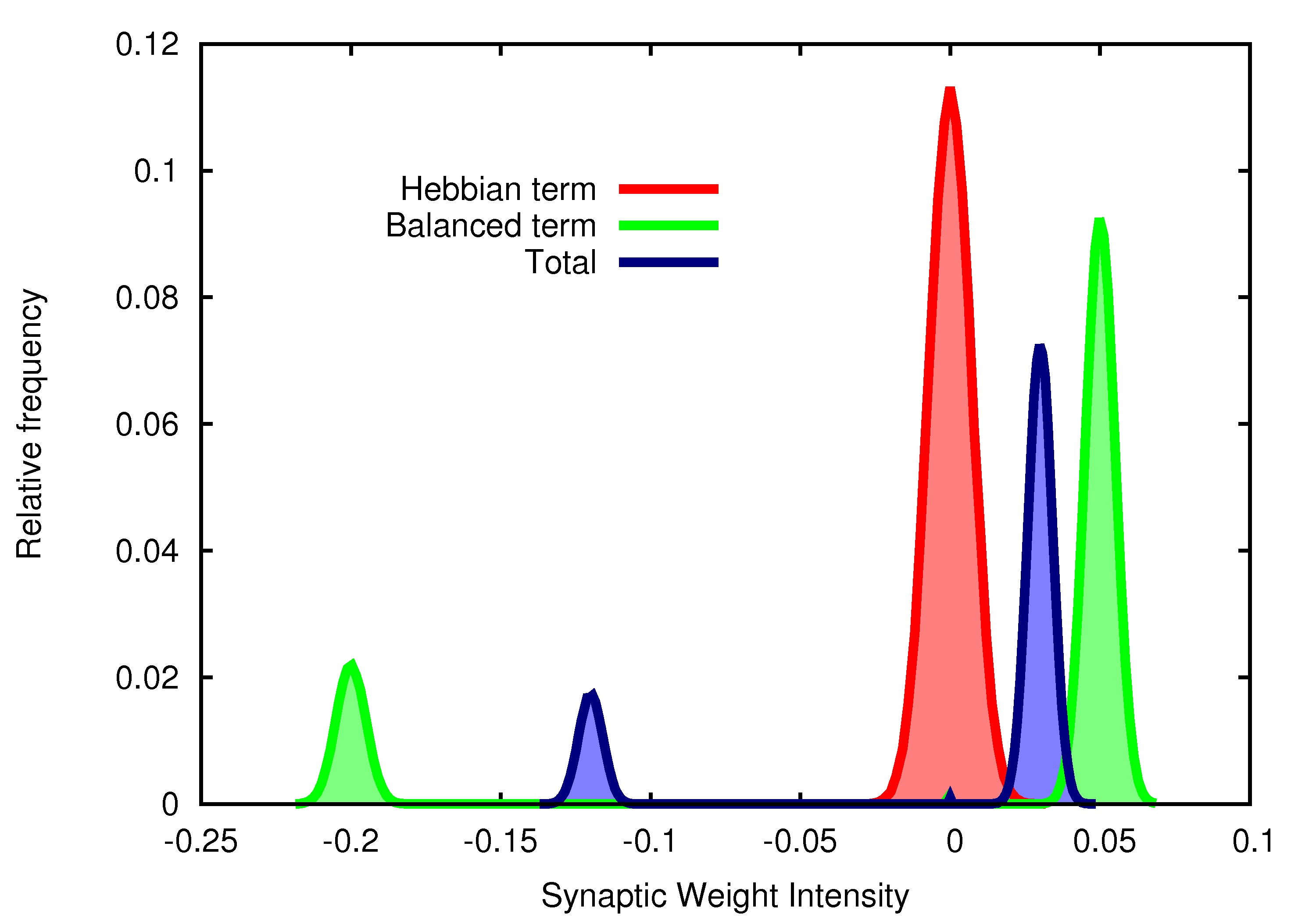
Figure 1: Generation of balanced I/E synaptic weight distributions including a Hebbian term. The red solid curve is the distribution of the synaptic weights $\omega_{ij}^{H}$ considering only a Hebbian term, which turns out to be approximatively a Gaussian distribution for a large number $P$ of unbiased random patterns [28]. On the other hand, the green solid curve represents a bimodal or balanced E/I non-Hebbian Gaussian distribution. We build this balanced distribution such that excitatory (positive) synaptic weights are more likely to occur (four times more) than inhibitory (negative) synaptic weights, and their strength (on average) is four times lower than the intensity of inhibitory synapses. Using these two distributions, we can build a balanced Hebbian distribution for a random variable which is the sum of a Hebbian random synaptic weight and a non-Hebbian random balanced synaptic weight according to (3). This final distribution (blue curve) still preserves the balance I/E and other features of the original non-Hebbian balanced distribution, whereas it includes Hebbian features that allow for associative memory tasks. Parameter values used to obtain different histograms were $N=1000,\,P=50,\,\kappa=1,\,\sigma=0.1$ and $c=0.4.$

The parameter $\eta$ measures the relative abundance of excitatory synapses compared with inhibitory ones. Although a complete study of the behavior of the system can be done as a function of this parameter (see next section), we consider in most of our analysis appropriate values of $\eta$ which can mimic actual conditions. For instance, for $\eta=0.8$ one obtains a balance between excitation and inhibition similar to that reported to be present in the cortex of human brain [14, 16, 15]. With this choice there is a $80\%$ of excitatory synapses and a $20\%$ inhibitory ones. The factor $\alpha$ in (6) has been included to impede the total synaptic current $h_{i}=\sum_{j}\omega_{ij}s_{j}\varepsilon_{ij}$ to diverge in the thermodynamic limit $(N\rightarrow\infty)$ (in some situations of interest this choice has to be done carefully, see for instance [29, 30] for a discussion concerning this issue). Finally, we define the threshold term appearing in equation (1) as $\theta_{i}=\frac{1}{2}\sum_{j}\omega_{ij}$, to recover in the limit of $c=1$ the standard Hopfield model in the $\{1,-1\}$ code (see for instance [31]).

We can calculate how well a stored pattern is retrieved by the network dynamics by means of the overlap function defined as

$$m^{\mu}(\mathbf{s})\equiv\frac{1}{Na(1-a)}\sum_{i}\left(\xi_{i}^{\mu}-a\right)\left(s_{i}-a\right).$$ (7)

Due to the symmetry pattern-antipattern inherent in the present model, a given memory $\mu$ will be retrieved during the dynamics of the system when $|m^{\mu}(\mathbf{s})|=1.$ We can also measure the activity of the neural network, that is, how many neurons are firing together at the same time, monitoring the order parameter

$$m(\mathbf{s})\equiv\frac{1}{N}\sum_{j}\left(2s_{j}-1\right).$$ (8)

This measure can be easily related with the mean network activity or mean firing rate $\nu(\mathbf{s})=\frac{1}{N}\sum_{i}s_{i}=\frac{m(s)+1}{2},$ in such a way that a solution with $m(\mathbf{s})=1$, corresponds to a neuron population with a high mean firing rate ($\nu=1$) (Up state) and $m(\mathbf{s})=-1$ corresponds with a silent neural population ($\nu=0$) (Down state).

In the next section we will report the main results of our study for the case of a single stored pattern ($P=1$) which allow for a simple mean-field theoretical treatment due to the lack of effects produced by the interference of a number of stored patterns scaling with $N.$

3 Results

3.1 Mean-field analysis

In order to develop a theoretical treatment of the model presented above, we have to note that the total synaptic weights (3) are intrinsically asymmetric due to the balanced term $\omega_{ij}^{B}$, so one can not use typical theoretical techniques from equilibrium statistical mechanics to derive self-consistent equations for the order parameters (see for instance [5]). However, since our system involves a fully connected network, we still can derive a standard mean-field description to find these self-consistent equations that will allow to monitor the behavior of the system as relevant control parameters change. We can start by computing the quenched and canonical ensemble average of some magnitudes of interest in their steady state using the thermodynamic limit $\left(N\rightarrow\infty\right)$. For example, for a given realization of the quenched disorder $\{\xi_{i}^{\mu},w_{ij}^{B}\}$ and from equation (7) the mean overlap function becomes

$$m^{\mu}\equiv\langle m^{\mu}(\mathbf{s})\rangle=\frac{1}{Na(1-a)}\sum_{i}\left(\xi_{i}^{\mu}-a\right)\left(\left\langle s_{i}\right\rangle-a\right),$$ (9)

where using (1) one obtains

$$\left\langle s_{i}\right\rangle=\frac{1}{2}\left[1+\tanh\left[2\beta\left(h_{i}-\theta_{i}\right)\right]\right].$$ (10)

For simplicity, in the following we will consider the case of a single stored random pattern $(P=1)$ with equal probability of having $1$ or $0$ for its elements, i.e. $p\left(\xi_{i}^{\mu}\right)=\frac{1}{2}\delta\left(\xi_{i}^{\mu}-1\right)+\frac{1}{2}\delta\left(\xi_{i}^{\mu}\right),$ which implies $a\equiv\langle\xi_{i}^{\mu}\rangle=\frac{1}{2}$, and then is straightforward to obtain

$$\begin{array}[]{c}2\left(h_{i}-\theta_{i}\right)=\frac{c}{N}\sum_{j}\left(2\xi_{i}^{\mu}-1\right)\left(2\xi_{j}^{\mu}-1\right)\left(2\left\langle s_{i}\right\rangle-1\right)+\left(1-c\right)\sum_{j}\omega_{ij}^{B}\left(2\left\langle s_{i}\right\rangle-1\right)\\ \\ =c\epsilon_{i}^{\mu}m^{\mu}+\left(1-c\right)Nm\omega_{i}^{B},\end{array}$$

where $\epsilon_{i}^{\mu}\equiv(2\xi_{i}^{\mu}-1)$ and

$$m\equiv\langle m(\mathbf{s})\rangle=\frac{1}{N}\sum_{j}\left(2\langle s_{j}\rangle-1\right).$$ (11)

In the last, we also assumed the particular case that $\omega_{ij}^{B}=\omega_{i}^{B}\;\forall j$, that is, the random contribution to all synapses toward a given postsynaptic neuron $i$ is of the same type (either excitatory or inhibitory) and has the same random value or strength. Note additionally that $\epsilon_{i}^{\mu}$ is also a random variable with probability $p(\epsilon_{i}^{\mu})=\frac{1}{2}\delta(\epsilon_{i}^{\mu}-1)+\frac{1}{2}\delta(\epsilon_{i}^{\mu}+1).$ We then finally can obtain the fixed point equations

$$\begin{array}[]{l}m^{\mu}=\frac{1}{N}\sum_{i}\epsilon_{i}^{\mu}\tanh\beta[c\epsilon_{i}^{\mu}m^{\mu}+(1-c)Nm\omega_{i}^{B}]\\ \\ m=\frac{1}{N}\sum_{i}\tanh\beta[c\epsilon_{i}^{\mu}m^{\mu}+(1-c)Nm\omega_{i}^{B}].\end{array}$$ (12)

In the thermodynamic limit $N\rightarrow\infty,$ one can assume self-averaging of both order parameters and, therefore, the sums $\frac{1}{N}\sum$ appearing in (12) can be replaced by averages over the joint distribution of quenched disorder $P(\epsilon,\omega^{B})=p(\epsilon)p(\omega^{B}),$ leading to

$$\begin{array}[]{l}m^{\mu}=\langle\langle\epsilon_{i}^{\mu}\tanh\beta[c\epsilon_{i}^{\mu}m^{\mu}+(1-c)Nm\omega_{i}^{B}]\rangle\rangle\\ \\ m=\langle\langle\tanh\beta[c\epsilon_{i}^{\mu}m^{\mu}+(1-c)Nm\omega_{i}^{B}]\rangle\rangle\end{array}$$ (13)

where $\langle\langle\cdot\rangle\rangle$ means average over $P(\epsilon,\omega^{B})$. Assuming moreover the case of small $\sigma$ ($\sigma\rightarrow 0$), the Gaussian distributions in (6) can be approached to delta distributions, that is

$$p(\omega_{i}^{B})\approx\eta\delta(\omega_{i}^{B}-\kappa/N)+(1-\eta)\delta(\omega_{i}^{B}+4\kappa/N).$$

We have checked in simulations other possible non-zero but small values of $\sigma$ and the main results presented in this work (see below) are not dramatically affected by this choice as long as the synaptic intensities are sharply distributed around the two main modes of (6). Note moreover that for $P=1$ one has $\alpha=1/N.$ Then, after computing the double angle averages, the system (13) becomes

$$\begin{array}[]{l}m^{\mu}=\frac{\eta}{2}\tanh\beta(cm^{\mu}+(1-c)\kappa m)+\frac{1-\eta}{2}\tanh\beta(cm^{\mu}-(1-c)4\kappa m)\\ \\ +\frac{\eta}{2}\tanh\beta(cm^{\mu}-(1-c)\kappa m)+\frac{1-\eta}{2}\tanh\beta(cm^{\mu}+(1-c)4\kappa m),\\ \\ m=\frac{\eta}{2}\tanh\beta(cm^{\mu}+(1-c)\kappa m)+\frac{1-\eta}{2}\tanh\beta(cm^{\mu}-(1-c)4\kappa m)\\ \\ -\frac{\eta}{2}\tanh\beta(cm^{\mu}-(1-c)\kappa m)-\frac{1-\eta}{2}\tanh\beta(cm^{\mu}+(1-c)4\kappa m),\end{array}$$ (14)

which in a more compact form can be written as

$$\begin{array}[]{c}m^{\mu}+m=\eta\tanh\beta(cm^{\mu}+(1-c)\kappa m)+(1-\eta)\tanh\beta(cm^{\mu}-(1-c)4\kappa m)\\ \\ m^{\mu}-m=\eta\tanh\beta(cm^{\mu}-(1-c)\kappa m)+(1-\eta)\tanh\beta(cm^{\mu}+(1-c)4\kappa m).\end{array}$$

One can solve numerically the steady-state equations (14) and find fixed point solutions for $m^{\mu}$ and $m$ as a function of the temperature parameter $T$ and for several values of the parameter $c$ (see below). However, one can analytically study some limits of interest. For example, let us consider the limiting case $c=1.$ In this situation, one recovers the mean field equation for the standard Mattis states of the Hopfield model [31]

$$\begin{array}[]{l}m^{\mu}=\tanh\beta m^{\mu}\\ \\ m=0.\end{array}$$

The first equation of the last expression has the trivial solution $m^{\mu}=0,$ which is the only one for large $T.$ For lower values of $T,$ this equation can be developed for small $m^{\mu}$ given a critical temperature $T_{cr}=1$ for the appearance of memory Mattis states ($m^{\mu}\neq 0$). On the other hand, for the limit $c=0$ one has

$$\begin{array}[]{l}m^{\mu}=0\\ \\ m=\eta\tanh\beta\kappa m-(1-\eta)\tanh 4\beta\kappa m.\end{array}$$ (15)

Then, for $c=0,$ there are not Mattis states (since $m^{\mu}=0$), so memories states are not present. However, other type of network activity states (not yet described in the literature) can emerge, namely the non-trivial solutions with $m\neq 0$ of the second equation of (15).

One easily can visualize that $m=0$ is a trivial solution of the second equation of (15), which is the only one present for very large $T.$ On the other hand, for $T=0$, one has that the equation for $m$ becomes $m=(2\eta-1)\mbox{sign}(m)$. Then, e.g, for the case of $\eta=0.8$, this gives a nontrivial Up state with $m=0.6\,(i.e.,\,\nu=0.8),$ and a Down state with $m=-0.6\,(i.e.,\,\nu=0.2).$ The critical temperature for the appearance of non-trivial solutions with $m\neq 0$ can be easily computed developing the second equation of (15) for small $m$ which gives

$$\overline{T}_{cr}=5\eta\kappa-4\kappa.$$

This results in a real critical temperature only when $\eta>4/5$ (independently of $\kappa$), and non-trivial solutions ($m\neq 0$) appear below such $\overline{T}_{cr}$ as in a continuous second order phase transition. Note that $\eta=0.8=4/5$ marks the limit for the appearance of this second order phase transition. That is, for larger values of the population of excitatory synapses, i.e, $\eta>0.8,$ the transition for the appearance of this non-trivial network activity states is second order. On the other hand, for $\eta\leq 0.8$ there is not such critical temperature, which implies a sharp first-order phase transition for the appearance of these non-trivial network activity states.

For $0<c<1,$ both type of solutions, that is Mattis memory states and the Up and Down activity states not correlated with stored memories, can also appear for different values of the temperature parameter $T,$ and can coexist as we will illustrate in the next section. In this more general scenario, one can derive also some analytic results as follows. By a simple inspection of equations (14) one can easily check that $m^{\mu}=0$ and $m=0$ is a trivial solution of the these steady-state equations, and that such solution appears for large $T,$ i. e. small $\beta,$ above some critical temperature. Making a Taylor expansion of equations (14) around this trivial solution one finds:

$$\begin{array}[]{l}m^{\mu}\approx\beta cm^{\mu}\\ \\ m\approx\beta(5\kappa\eta-4\kappa)(1-c)m.\\ \\ \end{array}$$

This gives again a critical temperature $T_{cr}=c$ for the appearance of memory Mattis states, and $\overline{T}_{cr}=(1-c)(5\kappa\eta-4\kappa)$ for the appearance of nontrivial states with $m\neq 0.$ Note that $T_{cr}\neq\overline{T}_{cr}$ which implies that states with $m^{\mu}\neq 0$, in general, do not correspond to states with $m\neq 0,$ or that states with $m^{\mu}=0$ are not usually associated with states with $m=0.$ Additionally, since the stored patterns have $\langle\xi_{i}^{\mu}\rangle=a=0.5,$ any time one reaches a steady state with $m^{\mu}\neq 0$, it will correspond to $m\approx 0$ and viceversa. It is worth noting to say that the cases $c=1$ and $c=0$ recover our previous findings above in these limits of interest. In particular, that $\overline{T}_{cr}$ is a true critical temperature only for $\eta>0.8$. It is important also to note that all results reported in next sections have been obtained for $\eta=0.8,$ so there is not such critical temperature $\overline{T}_{cr}.$ In this situation, the transition between states with $m\neq 0$ and states with $m=0$ occurs as in a first order transition at a temperature that we denote as $T_{t}$ (see next section).

3.2 Linear stability analysis and phase diagram

The dynamics of our system can be easily derived from equation (1) yielding to

$$\langle s_{i}\rangle_{t+1}=\frac{1}{2}\left[1+\tanh\left[2\beta\left(h_{i}(t)-\theta_{i}\right)\right]\right].$$

After using the same analysis and approaches done in section 3.1, this dynamics results in the coupled iterative map:

$$\begin{array}[]{l}m^{\mu}(t+1)=\frac{\eta}{2}\tanh\beta(cm^{\mu}(t)+(1-c)\kappa m(t))+\frac{1-\eta}{2}\tanh\beta(cm^{\mu}(t)-(1-c)4\kappa m(t))\\ \\ +\frac{\eta}{2}\tanh\beta(cm^{\mu}(t)-(1-c)\kappa m(t))+\frac{1-\eta}{2}\tanh\beta(cm^{\mu}(t)+(1-c)4\kappa m(t)),\\ \\ m(t+1)=\frac{\eta}{2}\tanh\beta(cm^{\mu}(t)+(1-c)\kappa m(t))+\frac{1-\eta}{2}\tanh\beta(cm^{\mu}(t)-(1-c)4\kappa m(t))\\ \\ -\frac{\eta}{2}\tanh\beta(cm^{\mu}(t)-(1-c)\kappa m(t))-\frac{1-\eta}{2}\tanh\beta(cm^{\mu}(t)+(1-c)4\kappa m(t)),\end{array}$$ (16)

which can be analyzed using standard techniques.

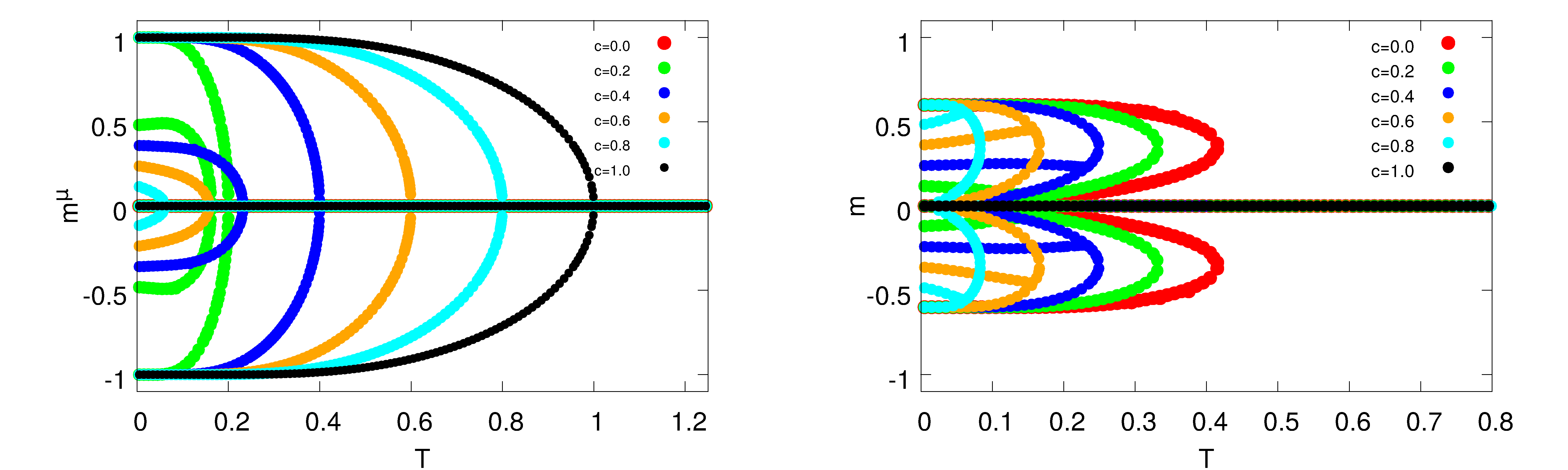
Figure 2: Mean-field fixed point solutions for the overlap (left) and for the mean network activity measured with $m$ (right) for different values of $c$. Each colored curve represents the behavior as a function of $T$ of all possible steady-state solutions (locally stable and unstable) for a given $c$ value. Note the symmetry between positive and negative solutions in both $m^{\mu}$(corresponding to pattern and antipattern solutions) and $m$ (corresponding to Up and Down activity states not correlated with a given stored pattern). Parameter values were $\kappa=1,\,\eta=0.8$ and $\sigma=0.$

Fixed point solutions of such map, as a function of the relevant parameters $T$ and $c$ are plotted in figure 2, which illustrates the complex and rich attractor structure of our system. However, not all of these fixed point solutions are stable so in simulations of the system some of them will no be reached in stationary conditions. To see the stability of these solutions and the bifurcation structure of our system in terms of $T$ and $c,$ we can perform, e.g., a standard linear stability analysis of the fixed point solutions. This implies that we have to diagonalize the resulting Jacobian Matrix $\mathbf{A}=(A_{ij})$ of the previous iterative map (16), that is

$$\begin{array}[]{l}A_{11}=\eta\beta c(\mathcal{B}_{+}^{\mu}+\mathcal{B}_{-}^{\mu})+(1-\eta)\beta c(\mathcal{C}_{+}^{\mu}+\mathcal{C}_{-}^{\mu})\\ \\ A_{12}=\eta\beta(1-c)\kappa(\mathcal{B}_{+}^{\mu}-\mathcal{B}_{-}^{\mu})+4(1-\eta)\beta(1-c)\kappa(\mathcal{C}_{+}^{\mu}-\mathcal{C}_{-}^{\mu})\\ \\ A_{21}=\eta\beta c(\mathcal{B}_{+}^{\mu}-\mathcal{B}_{-}^{\mu})-(1-\eta)\beta c(\mathcal{C}_{+}^{\mu}-\mathcal{C}_{-}^{\mu})\\ \\ A_{22}=\eta\beta(1-c)\kappa(\mathcal{B}_{+}^{\mu}+\mathcal{B}_{-}^{\mu})-4(1-\eta)\beta(1-c)\kappa(\mathcal{C}_{+}^{\mu}+\mathcal{C}_{-}^{\mu})\\ \\ \mathcal{B}_{\pm}^{\mu}=\frac{1}{2}[1-\tanh^{2}\beta(cm^{\mu}\pm(1-c)\kappa m)];\,\mathcal{C}_{\pm}^{\mu}=\frac{1}{2}[1-\tanh^{2}\beta(cm^{\mu}\pm(1-c)4\kappa m)].\end{array}$$

The local stability criterion for a given steady state solution, let say ($(m^{\mu})^{*},m^{*}$), then is $|\lambda|_{max}=max_{i}|\lambda_{i}|<1,$ where $\lambda_{i}$ are the eigenvalues of $\mathbf{A}$ evaluated in the solution ($(m^{\mu})^{*},m^{*}$). Using this criterion we depict with different colors in figure 3 and 4, the stability of the steady-state solutions previously illustrated in figure 2. Blue colors corresponds to unstable solutions, that is, solutions such that $|\lambda|_{max}\geqslant 1,$ whereas red, orange and green solutions are locally stables, that is, for these solutions one has $|\lambda|_{max}<1.$ Both figures show that below certain transition temperature $T_{t}$ and for certain range of $c$ values, metastability or multistability can emerge in the system (there are more than one fixed-point solution which are locally stable for the same value of temperature). Metastable solutions are depicted, for instance, in top panels of figures 3 and 4, whereas multistability is shown in middle panels and left bottom panel of these figures. More precisely, the stable memory attractors (red solutions) – that have $m^{\mu}\neq 0$ and $m=0$ – remain stable or metastable (orange or green solutions in figure 3) below $T_{t}$ and, additionally, a stable non-memory solution emerges also below $T_{t}$. These correspond to the orange and red solutions with $m^{\mu}=0$ and $m\neq 0$ appearing for $T<T_{t}$ in figure 3 (see also figure 4).

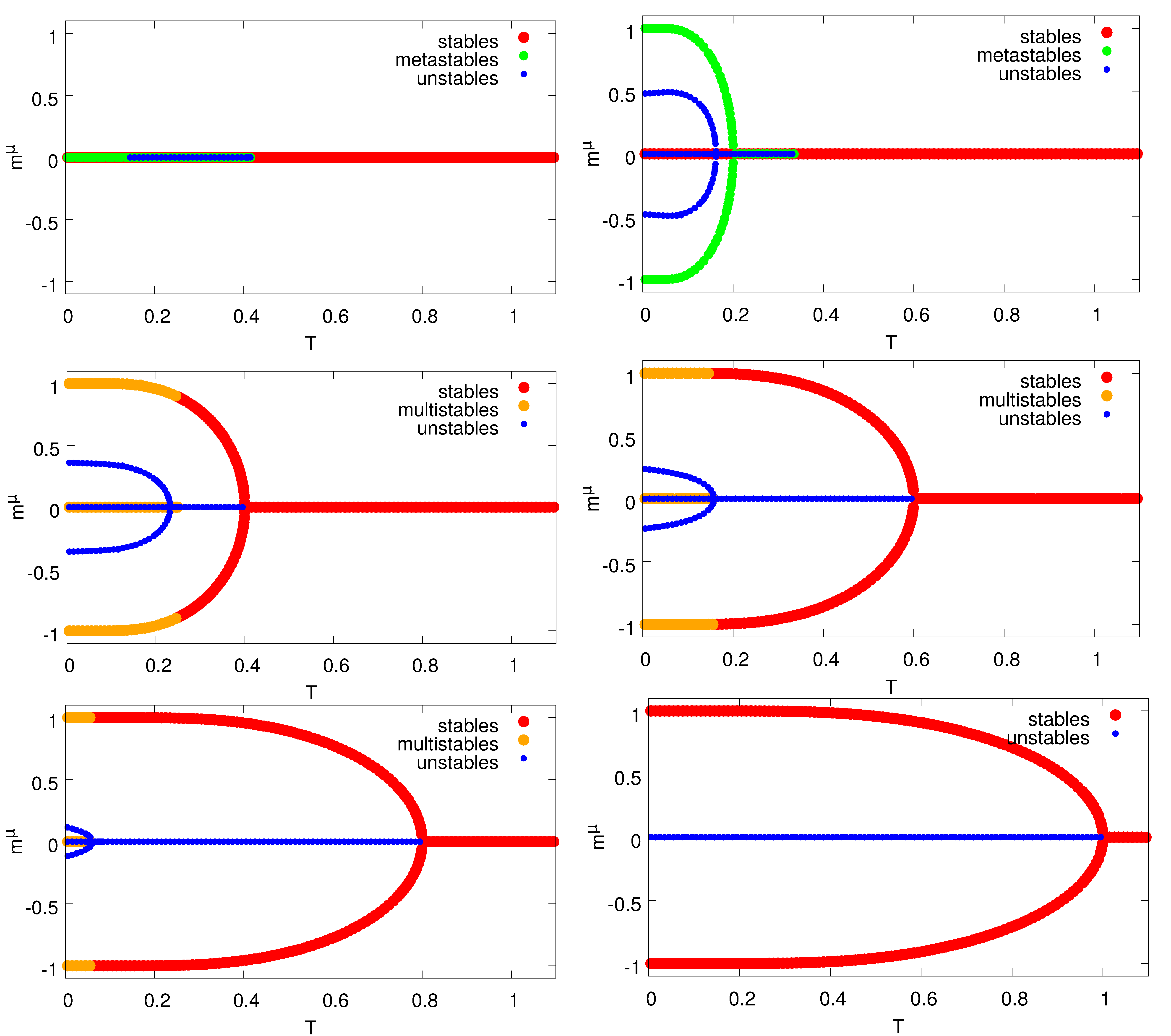
Figure 3: Description of the local-stability of the overlap fixed point solutions. Different steady solutions of the overlap function $m^{\mu}$ for different values of $c$ are depicted. The values of $c$ used, starting from top left to bottom right panels, are $c=0.0\>c=0.2\>c=0.4\>c=0.6\>c=0.8\>c=1.0$. Bottom right figure shows the fixed-point solutions and their stability for the standard Hopfield case $c=1$. Other panels corresponds to the case in which balanced contribution to the synaptic weights is present with probability $c.$ Parameter values have been taken as in figure 2.

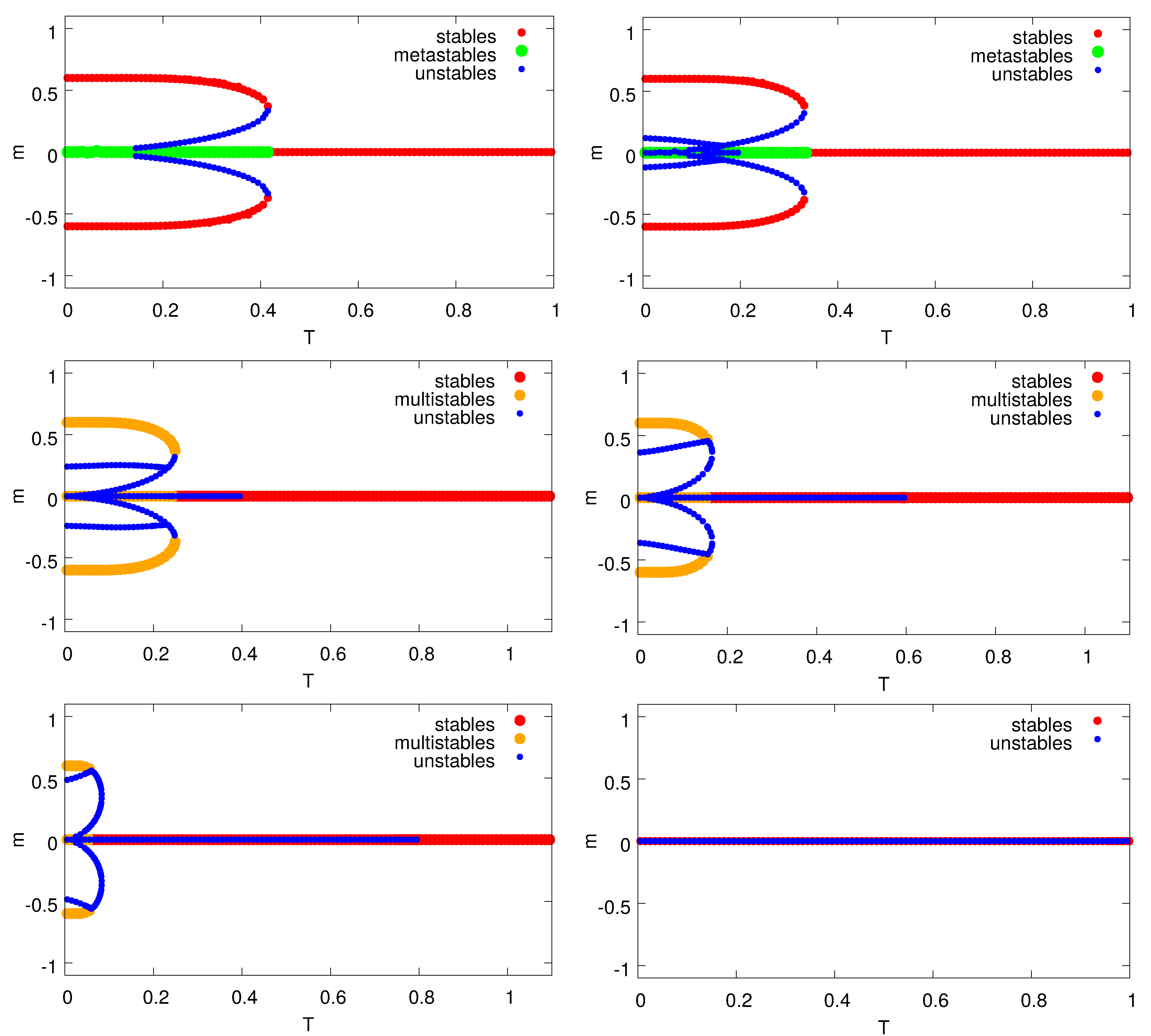
Figure 4: Stability of mean network activity fixed-point solutions. Each panel illustrates different steady-state solutions of the mean network activity $m$ for different values of $c$. The values of $c$ used starting from top-left to bottom-right panels are $\left[c=0.0\>c=0.2\>c=0.4\>c=0.6\>c=0.8\>c=1.0\right]$. Bottom right panel shows the traditional Hopfield model solution where the synaptic weights are computed according to Hebb rule $(c=1)$. The figures clearly depict that in addition to a locally stable zero $m$ solution, others locally stable non-zero fixed-point solutions of $m$ emerge at very low temperatures below certain transition temperature $T_{t},$ as in a first order phase transition. This fact results in multistability or metastability in the system just below $T_{t}.$

Figure 5: Phase diagram depicting different phases in our system. For $T<T_{cr}=c$ (solid and dotted line) stable memory states appear as in a second order phase transition. For $T<T_{t}$ (dashed line) frustrated states emerge that are the only present in the system for $T>T_{cr}$ and that can coexist with the memory states for $T<T_{cr}.$ Parameter values have been taken as in figure 2.

Using the stability criterion explained above we have computed the whole phase diagram ($T,c$) of our system for $\kappa=1$ and $\eta=0.8,$ which is depicted in figure 5. This shows a paramagnetic or non-memory phase (gray color) at high temperature for the whole range of $c.$ As $T$ decreases a memory phase (dark green color) emerges as in a second order phase transition at the critical temperature $T_{cr}=c$, (solid and dotted lines). In addition, also for low values of temperature a frustrated phase with non-memory attractors emerges as in a sharp first-order transition below some transition temperature $T_{t}=f(c)$ for all values of $c$ (dashed line). For $T<T_{t}$ and $T<T_{cr}$ (dark blue region) frustrated solutions coexist with the memory ones, in such a way that for $c\apprle 0.3$ frustrated solutions are the global minima of the dynamics, being memory solutions metastable, whereas for $c\apprge 0.3$ multistability among frustrated and memory states is present. Note that for $T<T_{t}$ and $T>T_{cr}$ , the frustrated phase is the only present in the system (light blue color region). This type of non-memory attractors differ from paramagnetic phase because of its high and low mean network activities. As will be show in the next section, all these mean-field results are confirmed by Monte Carlo simulations of our system.

3.3 Monte Carlo simulations versus mean-field results

Monte Carlo simulations of our system are in agreement with the mean field results described above for the whole range of the parameters $T$ and $c$ we can consider, as the figures 6 and 7 clearly depict. In these figures we only represent the positive solutions for $m^{\mu}$ and $m$ as a function of $T$ and $c,$ but it is worth noting to say that due to the symmetry $1,0$ for the state variables $s_{i}$ and stored patterns $\xi_{i}^{\mu},$ exact symmetric negative solutions for $m^{\mu}$ and $m$ are also present in the steady state of the system not only in the mean-field results reported above but also in simulations. In both figures, the blue solid lines correspond to the steady-states obtained using the analytic treatment (mean-field approach) described in the previous section, while the red data points are the steady-state solutions obtained from the Monte Carlo simulations for a network with $N=1600$ neurons. For a given value of $T$ and $c,$ these points have been obtained for 50 realizations of the system, after averaging time-series data points during a time window $\Delta t=500$ Monte Carlo steps (MCS) in the final steady-state. On the other hand, the solid green curves has been calculated averaging the resulting steady states (red points) over the 50 realizations of the simulated system, where error bars represent the corresponding standard deviations.

The figure 6 shows the behavior of the steady-state overlap function $m^{\mu}$ as a function of the temperature $T$ for different values of the parameter $c$. It clearly illustrates the appearance of frustrated states at low temperature where memory is lost ($m^{\mu}=0$) for $T<T_{t}$ and where a new phase with Up and Down activity states can emerge (see also 7). As in the mean-field results described in the previous section, in simulations these frustrated states appears for any $c<1,$ and are the only stable states for $c\lesssim 0.3$ (see for instance the two top panels in figure 6 and the inset in the top-right panel). The bottom-right panel of figure 6 corresponds to the traditional behavior of the Hopfield model ($c=1)$, where there is no contribution of the synaptic balanced term. In this case, one observes the expected memory retrieval curve as a function of $T$, where memory recall becomes less effective as $T$ increases below the critical temperature $T_{cr}=1$. As the parameter $c$ decreases, the term due to the balanced synaptic distribution becomes more important and the critical temperature $T_{cr}$ goes down – in fact as $T_{cr}=c$ – since these synaptic balanced terms act like a noise affecting the associative memory property. The range of $T$ at which the associative memory emerges is also narrower as $c$ decreases until it disappears for $c\lesssim 0.3.$ In this situation, in fact, memory attractors become metastable and the final steady-state is a frustrated one (see inset in the top-right panel). Thus, e.g., for the other limit $c=0$, the associative memory property is completely lost – even metastable memory attractors are not present – since there is no contribution of the distribution governed by the Hebbian rule.

On the other hand, figure 6 also depicts that the averaged steady-state positive overlap over different system realizations (green solid line) has a reentrant behavior as a function of $T$ for $0.3<c<1.$ More precisely, for large $T$ the system falls into the paramagnetic or non-memory phase so this averaged overlap is zero. For values of $T<T_{cr},$ the averaged overlap follows the memory recall curve that tries to saturate to its maximum value $1$ as $T$ decreases. This occurs until $T<T_{t}$ where the averaged overlap again goes toward a small value near zero. This is due to the existence of many frustrated states (with $m^{\mu}\approx 0$) compared with the number of steady-states that reach the stored pattern (with $m^{\mu}\approx 1$). Moreover, the number of realizations that put the system in the basin of attraction of the memory state decreases as $T$ is lowered which is an indication that the basin of attraction of the memory states diminishes below $T_{t}$ when $T\rightarrow 0.$ As soon as the relevance of the balanced term is more important this quasi-reentrant transition becomes more prominent (see the left-middle panel of figure 6 for $c=0.4$).

Figure 6: Overlap vs Temperature. Each panel shows the behavior of the overlap function $m^{\mu}$ for different values of $c=0,\,0.2,\,0.4,\,0.6,\,0.8,\,1$ (increasing from top-left to bottom-right). The top left figure $(c=0)$ is the situation where the Hebbian term in absent, while the bottom right figure $(c=1)$ is the opposite situation, where only the Hebbian term rules the synaptic strength. Blue solid line represent the mean-field steady-state of the system. Red points corresponds to the final time-averaged steady-state of the system for 50 realizations of the simulated systems with $N=1600$ neurons, whereas the green solid line is the averaged steady-state over these 50 realizations of the system (error bars correspond to the standard deviations of the 50 data points).

The above mean-field and simulation findings can be easily understand since we are introducing a random contribution, with probability $(1-c),$ to the synaptic weights which does not depend on the stored patterns. It is expected, therefore, that memory retrieval capacity of the system decreases as $c\rightarrow 0.$ The reason is that the mechanism involved to achieve the recall of memories in auto-associative networks is due to the correlation between the stored patterns $\xi_{i}^{\mu}$ and the current network activity $s_{i}$ state, and the information content of memories is only present in the Hebbian term. Memory recall capacity then decreases in a way that the critical temperature for the appearance of Mattis states gets smaller as the random disorder introduced by the bimodal contribution increases. This is clearly depicted in the left-top panels of figures 3 and 6, where it can be observed how the total absence of Hebbian contribution in the learning rule, turns into memory frustration due to the total lack of correlation between the patterns and the synaptic weights.

As described above, simulations, in agreement with mean-field results, shows the existence of a new intriguing region at low temperatures (for $c<1$ below $T_{t}$) where the memory is frustrated (that is, $m^{\text{$\mu$}}=0$) and where other type of order is present (with $m\neq 0$) as it is depicted in figures 4 and 7. Note that in the memory phase one has $m=0$ since we have chosen the learned pattern such that $\langle\xi_{i}^{\mu}\rangle=1/2$. This new frustrated phase emerges sharply lowering the $T$ from the stable memory phase as in a first order phase transition. One could interpret this transition as a re-entrant phase transition from a memory phase to a non-memory phase at low temperatures as in traditional equilibrium and non-equilibrium spin-glass models [32, 33, 34, 35], which in our case is of first order type. An important difference with respect to previous studies, as in the traditional (equilibrium) Hopfield model, is that the SG frustrated behavior is achieved for infinitely large number of stored patterns, i.e. $\alpha>0$. Our results here shows that frustrated states can be achieved also in the case of $\alpha\rightarrow 0$ for our model, when one assumed a balance condition for synaptic weights and certain homogeneity among the synaptic intensities of the afferents for a given postsynaptic neuron.

Figure 7: Mean Network Activity vs Temperature for the same cases depicted in figure 6. Each figure shows the behavior of the mean network activity, as measured with the order parameter $m,$ for different values of $c$. Again, from top to bottom, the figure depicts the steady state solutions that the system reaches both in simulations (red data points) and within our mean field theory (blue solid lines) as a function of $T,$ for increasing values of the parameter $c.$

Also in agreement with mean-field results above is the finding in simulations that in this new phase, $m$ increases (decreases in the case of the negative solution) as $T$ decreases until a value of $m\approx 0.6$ (or $-0.6$ in the case of the negative solution) at $T=0.$ Moreover, simulations depict that this frustrated phase gets wider in the temperature range for $c\rightarrow 0$ and, therefore $T_{t}$ rises from zero as $c$ decreases reaching the value of $T_{t}\simeq 0.42$ at $c=0$ – see also the dashed line in figure 5. In terms of the mean firing rate $\nu,$ as we already mentioned, the positive solution for $m$ corresponds with an Up state that has a larger mean network activity (around $\nu\approx 0.8$) which indicates a state with a large population of firing neurons, whereas the symmetric negative solution corresponds to a Down or silent state with very low network activity (around $\nu\approx 0.2$). On the other hand, it is worth noting that memory states corresponds to a state with average network activity around $0.5,$ i.e., a steady state with approximately the same number of firing and silent neurons.

In order to describe how frustration arises in these low-temperature non-memory states, first we have checked if the steady-state averaged overlap depends of the initial conditions. For a given realization “$k$” of synaptic intensities, namely $\mathbf{\omega}^{k}=\left\{\omega_{ij}^{k}\right\}$, and given values of the parameters $T$ and $c,$ we found that overlap mean-value of the frustrated state remains the same for different simulation initial conditions (data not shown). This indicates that the system has only a minimum attractor associated to this frustrate state. However, when one chooses different realizations of the synaptic disorder one finds different values of the overlap mean value in the frustrated state as it is depicted in figure 8Left. This is an indication that the particular choice of the configuration of synapses determines the features of the reached frustrated state as in traditional spin-glass states. Due to the homeostatic balance (more excitatory synapses, but stronger inhibitory synapses) the synaptic intensities obey a constraint of the type, $\langle\omega_{ij}\rangle\equiv\frac{1}{N^{2}}\sum_{i,j}\omega_{ij}=0$. However, in our simulations $\langle\omega_{ij}\rangle$ is not exactly zero consequence of the network finite-size, and the variability found in the steady-state overlap mean-value of the frustrated solutions is not correlated with the dispersion of $\langle\omega_{ij}\rangle$ from zero as figure 8Left clearly depicts. This demonstrates that dispersion of reached frustrated states has not its origin in this finite-size effect and only is consequence of the intrinsic synaptic disorder introduced by the balanced term.

Secondly, we have computed the size of fluctuations over different realizations of synaptic disorder, for both memory and frustrated states in the multistable region, for $c=0.4$ and different temperature values, as it is shown in figure 8Right. More precisely, we computed

$$\begin{array}[]{l}{\displaystyle\Sigma^{2}=\frac{1}{N_{r}}\sum_{k=1}^{N_{r}}\left(m_{k}^{\mu}-\overline{m^{\mu}}\right)^{2}}\end{array}$$

where $N_{r}$ is the number of realizations, $m_{k}^{\mu}$ is the time-averaged overlap in the steady-state for a given synaptic disorder realization “$k$”, $\overline{m^{\mu}}\equiv\frac{1}{N_{r}}\sum_{k=1}^{N_{r}}m_{k}^{\mu}$ is the average of $m_{k}^{\mu}$ over different realizations of the synaptic disorder, and $\Sigma^{2}$ is the variance of $m_{k}^{\mu}$ also over different realizations of the synaptic disorder. This figure illustrates how fluctuations in the frustrate state are less sensible to temperature and remains even for very low temperature. The figure also depicts that $\Sigma$ mainly depends on network size. Moreover, there is a tendency to saturate the intensity of fluctuations toward a non-zero value for very large $N$ (see blue curves in figure 8Right and in its inset). In the case of memory states, however, fluctuations intensity decreases quickly with temperature until a zero value (see red curves in figure 8Right and in the inset). These findings indicate that the frustrated state fluctuations might also appear also in absence of thermal noise and in the thermodynamic limit and, therefore, are only due to the synaptic heterogeneity introduced by the balanced synaptic term.

Figure 8: Frustrated vs memory state fluctuations. Left panel depicts differences in the final frustrated state (measured in terms of the overlap $m^{\mu}$) over different realizations of the synaptic intensities, where $|\langle\omega_{ij}\rangle|$ is the absolute value of the mean synaptic strength of a given realization of synaptic intensities through the whole network. Right panel depicts the total size of the fluctuations of the steady state as a function of the network size and different values for the temperature (different symbols) for both, frustrated states (blue solid lines) and for memory states (red solid lines). The inset shows a zoom of the large $N$ behavior of different lines which illustrates the saturation of the size of the fluctuations for the frustrated states. Temperature values considered were $T=10^{-3}(\CIRCLE),\,0.05(\blacksquare),\,0.1(\blacklozenge),\,0.15(\blacktriangle),\,0.2\,(\bigstar),$$0.25$(✚),$0.3$(✖).

4 Conclusion

In traditional autoassociative neural networks, as the Hopfield model, the associative memory property is achieved by storing in the synaptic weights the information to be learned by means of a Hebbian learning prescription. In these models, each synaptic weight connects two different neurons and its strength reflect the correlation between the activity of those neurons during the activation of the learned pattern configuration. It can be easily demonstrated that when the number of stored patterns is very large, and these patterns are random and unbiased, the probability to have a given synaptic strength value becomes Gaussian centered around zero. This fact implies that in these models one has the same probability to have excitatory and inhibitory synapses, contrary with what is observed in nature, and that excitatory (or inhibitory) synapses with a large strength are rare, that is, almost all synapses have, in absolute value, a small value around zero.

In the present study, we have introduced a more realistic balanced synaptic term – with probability ($1-c$) – in addition to the standard Hebbian one (which then occurs with probability $c$). The resulting probability distribution for the synaptic weights $\omega_{ij}$ has more actual features, including an appropriate balance 4:1 between excitation and inhibition, and large synaptic strengths of the inhibitory synapses compared with the excitatory ones, as it has been described in actual neural systems [16, 15]. In addition, we consider that the introduced balanced term does not include information nor correlation with the stored patterns, so it acts as a “balanced synaptic noise” against the memory order induced by the Hebbian term.

As a consequence, the resulting model has new intriguing emerging phenomena not observed in the standard Hopfield model. For instance, for any value of $c<1,$ at low temperatures, a regime of memory frustration arises as in a first order phase transition below some transition temperature $T_{t}$. This kind of frustration resembles to that of a spin glass (SG) state, where due to the randomness of the $\omega_{ij}$ and the absence of significant thermal fluctuations, the network state can not retrieve any pattern and memory vanishes. However, the appearance of SG like solutions in the standard Hopfield model is restricted to the pattern saturation limit (that is $P\rightarrow\infty$ in the thermodynamic limit $N\rightarrow\infty$) which is not the case in our study, since frustrated states appears even for $\alpha=P/N=0$ ($P$ finite in the thermodynamic limit). It is worth noting to say here that SG solutions can appear also in Hopfield like models for $\alpha\rightarrow 0$ when the number of stored patterns scale with $N$ as $P\sim N^{k}$ with $k<1$ [36, 37] (which is not the case either in our system).

At large temperature, the system undergoes a standard second-order phase transition from the ferromagnetic (or memory) solutions to paramagnetic (no-memory) ones at a critical temperature $T_{cr}=c$. This means that the non-memory phase appears at lower temperatures as $c\rightarrow 0$. That is, the importance of the “balanced synaptic noise” diminishes the memories attractor stability, so that thermal agitation needs lower temperatures to destroy the memory and enter the system in a paramagnetic phase.

Our main findings in this work observed by means of the Monte Carlo simulations can be also be understand within a standard mean-field approach of the model. In fact, a simple linear stability analysis of the resulting mean-field dynamical equations demonstrated the existence of a locally stable non-memory phase at large temperature above $T_{cr},$ a locally stable memory phase below this critical temperature and multistability between memory and frustrated states at low temperature below $T_{t}$ and intermediate values of $c$. On the other hand, for low $c$, our analysis depicts that this multistable region transform in another where the stable memory attractor becomes metastable in such a way that the frustrated state becomes the global attractor of the dynamics.

Although we only present results concerning the case of $\alpha\rightarrow 0,$ possible generalizations of the present study for $\alpha\neq 0$ could be thought using replica-like formalisms as in [38, 39]. In this case, an important point to address is the relation between the frustrated states we found in our work and different type of spin-glass solutions emerging from the interference among many stored patterns [40]. Also interesting is the possible relation of the frustrated states we found in our system with the so called elusive spin-glass states recently reported in [41]. These states correspond only to a true spin-glass phase when the system is prepared in an out of equilibrium state. In fact, our frustrated states only appear for $c<1$ that correspond to the case of asymmetric weights and therefore no Hamiltonian description is possible.

Other important point in the present study is that the observed frustrated states appearing at low temperature are associated with two different levels of non-zero neuronal activity which is not correlated to that of the stored patterns (since when the patterns are retrieved the network activity becomes almost zero). These states, with relative high and low activity, could be associated to the well known “Up” and “Down” states previously described in simple models of interacting E/I neuron populations [42] and widely observed in the cortical activity of the mammals [43, 44]. Our theoretical framework in this work could be easily extended to include some destabilizing mechanisms of these states – as for instance including features of the hyperpolarizing potassium slow currents or dynamic synapses – which can induce transitions among then similar to those observed in actual neural systems [19, 45, 46, 21, 22].

Finally, some of the results and conclusions reported in the present work could be used to design new paradigms of artificial neural networks with possible applications in many fields such as robotics, artificial intelligence, optimization methods, etc (see for instance [47] and references therein).

5 Acknowledgments

The present work has been done under project FIS2013-43201-P which is funded by the Spanish Ministry of Economy and Competitiveness (MINECO) and by the European Regional Development’s Founds (FEDER). The authors also thank J. Marro, P. L. Garrido and P. I. Hurtado for valuable comments and suggestions.

References

- [1] J. J. Hopfield. Neural networks and physical systems with emergent collective computational abilities. Proc. Natl. Acad. Sci. USA, 79:2554–2558, 1982.
- [2] D. O. Hebb. The Organization of Behavior: A Neuropsychological Theory. Wiley, 1949.
- [3] M.V. Tsodyks. Associative memory in neural networks with the hebbian learning rule. Modern Physics Letters B, 03(07):555–560, 1989.
- [4] D. J. Amit. Modeling brain function: the world of attractor neural network. Cambridge University Press, 1989.
- [5] P. Peretto. An Introduction to the modeling of neural networks. Cambridge University Press, 1992.
- [6] S. E. Bosch, J. F. M. Jehee, G. Fernández, and Ch. F. Doeller. Reinstatement of associative memories in early visual cortex is signaled by the hippocampus. J. Neurosci., 34(24):7493–7500, 2014.
- [7] J. X. Wang, L. M. Rogers, E. Z. Gross, A. J. Ryals, M. E. Dokucu, K. L. Brandstatt, M. S. Hermiller, and J. L. Voss. Targeted enhancement of cortical-hippocampal brain networks and associative memory. Science, 345(6200):1054–1057, 2014.
- [8] D. A. Gutnisky and V. Dragoi. Adaptive coding of visual information in neural populations. Nature, 452(7184):220–224, 2008.
- [9] M.A. Castro-Alamancos, J.P. Donoghue, and B.W. Connors. Different forms of synaptic plasticity in somatosensory and motor areas of the neocortex. J. Neurosci., 15(7 Pt 2):5324–5333, 1995.
- [10] T. Takeuchi, A. J. Duszkiewicz, and R. G. M. Morris. The synaptic plasticity and memory hypothesis: encoding, storage and persistence. Phil. Trans. Roy. Soc. Lond. B: Biol. Sci., 369(1633), 2013.
- [11] E.T. Rolls and L.L. Baylis. Gustatory, olfactory, and visual convergence within the primate orbitofrontal cortex. J. Neurosci., 14(9):5437–5452, 1994.
- [12] N. N. Urban and G. Barrionuevo. Induction of hebbian and non-hebbian mossy fiber long-term potentiation by distinct patterns of high-frequency stimulation. J. Neurosci., 16(13):4293–4299, 1996.
- [13] R. F. Galán, M. Weidert, R. Menzel, A. V. M. Herz, and C. G. Galizia. Sensory memory for odors is encoded in spontaneous correlated activity between olfactory glomeruli. Neural Computation, 18(1):10–25, 2006.
- [14] Yousheng Shu, Andrea Hasenstaub, and David A. McCormick. Turning on and off recurrent balanced cortical activity. Nature, 423(6937):288–293, May 2003.
- [15] M. Okun and I. Lampl. Balance of excitation and inhibition. Scholarpedia, 4(8):7467, 2009.
- [16] J. E. Heiss, Y. Katz, E. Ganmor, and I. Lamp. Shift in the balance between excitation and inhibition during sensory adaptation of s1 neurons. J. Neurosci., 28:13320–13330, 2008.
- [17] V.S. Dani, Q. Chang, A. Maffei, G.G. Turrigiano, R. Jaenisch, and S.B. Nelson. Reduced cortical activity due to a shift in the balance between excitation and inhibition in a mouse model of rett syndrome. Proc. Nat. Acad. Sci. USA, 102(35):12560–12565, 2005.
- [18] A. Destexhe, S. W. Hughes, M. Rudolph, and V. Crunelli. Are corticothalamic ’up’ states fragments of wakefulness? Trends in Neurosciences, 30(7):334–342, 2007.
- [19] L. Pantic, J. J. Torres, H. J. Kappen, and S. C. A. M. Gielen. Associative memmory with dynamic synapses. Neural Comput., 14:2903–2923, 2002.
- [20] J. M. Cortes, J. J. Torres, J. Marro, P. L. Garrido, and H. J. Kappen. Effects of fast presynaptic noise in attractor neural networks. Neural Comput., 18:614–633, 2006.
- [21] J. F. Mejias, H. J. Kappen, and J. J. Torres. Irregular dynamics in up and down cortical states. PLoS ONE, 5(11):e13651, 2010.
- [22] J.M. Benita, A. Guillamon, G. Deco, and M. V. Sanchez-Vives. Synaptic depression and slow oscillatory activity in a biophysical network model of the cerebral cortex. Frontiers in Computational Neuroscience, 6(64), 2012.
- [23] M. V. Tsodyks and M. V. Feigel’man. The enhanced storage capacity in neural networks with low activity level. EPL (Europhysics Letters), 6(2):101, 1988.
- [24] G. G. Turrigiano and S. B. Nelson. Homeostatic plasticity in the developing nervous system. Nat. Rev. Neurosci., 5(2):97–107, Feb 2004.
- [25] P. R. Huttenlocher and C. de Courten. The development of synapses in striate cortex of man. Hum. Neurobiol., 6(1):1–9, 1987.
- [26] G. Chechik, I. Meilijson, and Eytan E. Ruppin. Synaptic pruning in development: A computational account. Neural Computation, 10(7):1759–1777, Oct 1998.
- [27] N.-J. Xu and M. Henkemeyer. Ephrin-b3 reverse signaling through grb4 and cytoskeletal regulators mediates axon pruning. Nat. Neurosci., 12(3):268–276, Mar 2009.
- [28] W. Feller. An Introduction to Probability Theory and Its Applications, Vol. 2, 2nd Edition. John Wiley & Sons, Inc.; 2nd edition, 1971.
- [29] E. Agliari, A. Barra, A. Galluzzi, D. Tantari, and F. Tavani. A walk in the statistical mechanical formulation of neural networks. arXiv:1407.5300v1 [cond-mat.dis-nn], 2014.
- [30] F. Guerra and L.F. Toninelli. The thermodynamic limit in mean field spin glass models. Communications in Mathematical Physics, 230(1):71–79, 2002.
- [31] D. J Amit, H. Gutfreund, and H Sompolinsky. Statistical mechanics of neural networks near saturation. Annals of Physics, 173(1):30–67, 1987.
- [32] S. F. Edwards and P. W. Anderson. Theory of spin glasses. Journal of Physics F: Metal Physics, 5(5):965–974, 1975.
- [33] D. Sherrington and S. Kirkpatrick. Solvable model of a spin-glass. Phys. Rev. Lett., 35:1792–1796, Dec 1975.
- [34] J. J. Torres, P. L. Garrido, and J. Marro. Modeling ionic diffusion in magnetic systems. Phys. Rev. B, 58:11488–11492, Nov 1998.
- [35] J. Marro and R. Dickman. Nonequilibrium Phase Transitions in Lattice Models. Cambridge University Press, 1999.
- [36] E. Agliari, A. Annibale, A. Barra, A. C. C. Coolen, and D. Tantari. Immune networks: multi-tasking capabilities at medium load. Journal of Physics A: Mathematical and Theoretical, 46(33):335101, 2013.
- [37] E. Agliari, A. Annibale, A. Barra, A. C. C. Coolen, and D. Tantari. Immune networks: multitasking capabilities near saturation. Journal of Physics A: Mathematical and Theoretical, 46(41):415003, 2013.
- [38] A. Barra, G. Genovese, F. Guerra, and D. Tantari. How glassy are neural networks? Journal of Statistical Mechanics: Theory and Experiment, 2012(07):P07009, 2012.
- [39] A. Barra, G. Genovese, and F. Guerra. The replica symmetric approximation of the analogical neural network. Journal of Statistical Physics, 140(4):784–796, 2010.
- [40] A. Barra, G. Genovese, and F. Guerra. Equilibrium statistical mechanics of bipartite spin systems. Journal of Physics A: Mathematical and Theoretical, 44(24):245002, 2011.
- [41] F. Krzakala, F. Ricci-Tersenghi, and L. Zdeborová. Elusive spin-glass phase in the random field ising model. Phys. Rev. Lett., 104:207208, 2010.
- [42] H. R. Wilson and J. D. Cowan. Excitatory and inhibitory interactions in localized populations of model neurons. Biophys. J., 12(1):1–24, 1972.
- [43] M. V. Sanchez-Vives and D. A. McCormick. Cellular and network mechanisms of rhythmic recurrent activity in neocortex. Nat. Neurosci., 3:1027–1034, 2000.
- [44] I. Timofeev, F. Grenier, M. Bazhenov, T. J. Sejnowski, and M. Steriade. Origin of slow cortical oscillations in deafferented cortical slabs. Cerebral Cortex, 10(12):1185–1199, 2000.
- [45] D. Holcman and M. Tsodyks. The emergence of up and down states in cortical networks. PLoS Comput. Biol., 2(3):174–181, 2006.
- [46] J. J. Torres, J.M. Cortes, J. Marro, and H.J. Kappen. Competition between synaptic depression and facilitation in attractor neural networks. Neural Comp., 19(10):2739–2755, 2007.
- [47] Pandian Vasant. Handbook of Research on Artificial Intelligence Techniques and Algorithms. IGI Global, 2016.