UV/IR Mixing In Non-Fermi Liquids: Higher-Loop Corrections In Different Energy Ranges

Abstract

We revisit the Ising-nematic quantum critical point with an $m$-dimensional Fermi surface by applying a dimensional regularization scheme, introduced in Phys. Rev. B 92, 035141 (2015). We compute the contribution from two-loop and three-loop diagrams in the intermediate energy range controlled by a crossover scale. We find that for $m=2$, the corrections continue to be one-loop exact for both the infrared and intermediate energy regimes.

I Introduction

Unconventional metallic states lying outside the framework of Laudau Fermi liquid theory have been the subject of intensive studies Holstein et al. (1973); Reizer (1989); Lee and Nagaosa (1992); Halperin et al. (1993); Polchinski (1994); Altshuler et al. (1994); Kim et al. (2008); Nayak and Wilczek (1994); Lee (2009); Sur and Lee (2014); Metlitski and Sachdev (2010a, b); Abanov and Chubukov (2004, 2000); Mross et al. (2010); Jiang et al. (2013); Dalidovich and Lee (2013); Sur and Lee (2015); Lawler et al. (2006); Mandal and Lee (2015); Eberlein et al. (2016); Chung et al. (2013); Wang et al. (2014) in the recent times. From the point of view of condensed matter systems, we want to construct minimal field theories that can capture universal low-energy physics, thus enabling us to understand the dynamics in controlled ways.

Non-Fermi liquids arise when a gapless boson is coupled with a Fermi surface. Depending on the system, the critical boson can carry zero momentum or some finite momentum. In the former case, examples include the Ising-nematic critical point Metlitski and Sachdev (2010a); Oganesyan et al. (2001); Metzner et al. (2003); Dell’Anna and Metzner (2006); Kee et al. (2003); Lawler et al. (2006); Lawler and Fradkin (2007); Rech et al. (2006); Wölfle and Rosch (2007); Maslov and Chubukov (2010); Quintanilla and Schofield (2006); Yamase and Kohno (2000); Yamase et al. (2005); Halboth and Metzner (2000); Jakubczyk et al. (2008); Zacharias et al. (2009); Kim et al. (2008); Huh and Sachdev (2008); Mandal and Lee (2015); Eberlein et al. (2016) and the Fermi surface coupled with an emergent gauge field Motrunich (2005); Lee and Lee (2005); Lee et al. (2006); Motrunich and Fisher (2007); Chung et al. (2013); Wang et al. (2014), when the fermions lose coherence across the entire Fermi surface. The latter scenario is realised in systems like the spin density wave (SDW) or charge density wave (CDW) critical points Metlitski and Sachdev (2010b); Abanov and Chubukov (2004, 2000); Sur and Lee (2015, 2016); Mandal (2016), where electrons on hot spots (or hot lines) play a special role because these are the ones which remain strongly coupled with the critical boson in the low energy limit. The above systems are examples of critical Fermi surfaces where the Fermi surfaces are well-defined through weaker non-analyticities (such as power-law singularities) of the electron spectral function Yin and Chakravarty (1996); Senthil (2008), although there is no finite jump or discontinuity in the electron occupation number as is seen in Fermi liquids. The Fermi surface at the quantum critical point is thus identified from a non-analyticity of the spectral function. The latter is inherited from that of the underlying Fermi liquid before the coupling with a gapless boson is turned on right at the quantum phase transition point. The effect of such coupling of the Fermi surface with critical bosons on potential pairing instability is another topic which has been examined carefully Chung et al. (2013); Wang et al. (2014); Metlitski et al. (2015); Mandal (2016).

In this paper, we will focus on the Ising-nematic quatum critical point. This system is worthy of investigation because there has been considerable experimental evidence that a nodal nematic phase occurs in certain cuprate superconductors in the underdoped regime, and probably a quantum phase transition occurs from this anisotropic state to an isotropic one. Measurements of strongly temperature-dependent transport anisotropies Ando et al. (2002) and neutron scattering experiments Hinkov et al. (2008) performed on such materials provide such evidence. Let us first review the dimensional regularization scheme that has been devised to study such critical points Dalidovich and Lee (2013); Mandal and Lee (2015). Denoting the dimension of Fermi surface by $m$ and the space dimensions by $d$, the number of spatial dimensions perpendicular to the Fermi surface is given by $(d-m)$. while $d$ controls the strength of quantum fluctuations, the $m$ tangential directions control the extensiveness of gapless modes. Tuning $d$, we can compute the upper critical dimension $d_{c}(m)$ as a function of $m$, such that theories below upper critical dimensions flow to interacting non-Fermi liquids at low energies, whereas systems above upper critical dimensions are expected to be described by Fermi liquids. In our earlier work in Ref. Mandal and Lee (2015), we have shown that theories with $m=1$ are fundamentally different from those with $m>1$. This is due to an emergent locality in momentum space that is present for $m=1$ Lee (2009). On the other hand, for non-Fermi liquids with $m>1$, any naive scaling based on the patch description is bound to break down as the size of Fermi surface ($k_{F}$) qualitatively modifies the scaling. This is the result of a UV/IR mixing, where low-energy physics is affected by gapless modes on the entire Fermi surface in a way that their effects cannot be incorporated within the patch description Mandal and Lee (2015).

In Ref. Mandal and Lee (2015), we identified the upper critical dimension $d_{c}(m)$ at which the one-loop fermion self-energy diverges logarithmically. Using $\epsilon=d_{c}(m)-d$ as an expansion parameter, we could perturbatively access the stable non-Fermi liquid states that arise in $d<d_{c}(m)$. While computing two-loop corrections, we found that there exists a crossover scale defined by the dimensionless quantity,

$$\lambda_{\text{cross}}\equiv\tilde{e}^{2}\,\left(\frac{k_{F}}{\Lambda}\right)^{m-1}\,,$$ (1)

where $\tilde{e}$ is the effective coupling constant which remains small during perturbative expansions and $\Lambda$ is the Wilsonian cut-off for energy scales and momenta away from the Fermi surface. For $m=1$, the $k_{F}$-dependence drops out from everywhere. Since $\tilde{e}\sim\mathcal{O}(\epsilon)$ within the perturbative window, one always deals with the limit

$$\lambda_{\text{cross}}<<1\quad\mbox{for}\,\,m=1\,.$$ (2)

The $m>1$ case is quite different. In the $\lambda_{\text{cross}}>>1$ limit for $m>1$, the higher-loop corrections have been shown to be suppressed by positive powers of $\tilde{e}$ and $\Lambda/k_{F}$. Due to this suppression by $1/k_{F}$, there is no logarithmic or higher-order divergence at the critical dimension. As a result, the critical exponents are not modified by the two-loop diagrams in the $k_{F}\rightarrow\infty$ limit. However, there exists a large energy window for small $\epsilon$ and $(m-1)$, before the theory enters into the low-energy limit controlled by $\lambda_{cross}>>1$. In this paper, we will carry out two-loop and three-loop calculations in this intermediate energy scale characterized by $\lambda_{cross}<<1$, in order to examine whether there are non-trivial quantum corrections from higher-loop diagrams for $m>1$. We will also compute those three-loop diagrams in the $\lambda_{\text{cross}}>>1$ limit and confirm that the $\Lambda/k_{F}$-suppression continues to hold as predicted in Ref. Mandal and Lee (2015).

The paper is organized as follows: In Sec. II, we revisit the action which describes the Ising-nematic quantum critical point for a system with an $m$-dimensional Fermi surface embedded in $d$ spatial dimensions, providing a way for achieving perturbative control by dimensional regularization. In Sec. III, we continue to review the renormalization group scheme applied for locating the infrared fixed point. In Sec. IV, we explain the crossover scale that governs the transition from infrared to intermediate energy scales. The counterterms obtained from two-loop diagrams are discussed in Sec. V, followed by a computation of the critical exponents in Sec. VI. We conclude with a summary and some outlook in Sec. VII. Details on the computation of the Feynman diagrams at two-loop and three-loop orders can be found in Appendices A and B respectively.

II Model

In the patch coordinate system used in Ref. Mandal and Lee (2015), the action for the Ising-nematic critical point involving an $m$-dimensional Fermi surface embedded in $d$ spatial dimensions, can be written as

$$S = \sum_{j}\int dk\bar{\Psi}_{j}(k)\Bigl{[}i{\mathbf{\Gamma}}\cdot{\mathbf{K}}+i\gamma_{d-m}\,\delta_{k}\Bigr{]}\Psi_{j}(k)\,\exp\Big{\{}\frac{{{\mathbf{L}}}_{(k)}^{2}}{\mu\,{\tilde{k}}_{F}}\Big{\}}+\frac{1}{2}\int dk~{}{{\mathbf{L}}}_{(k)}^{2}\,\phi(-k)\,\phi(k)$$ (3)

$$+\frac{i\,e\,\mu^{x/2}}{\sqrt{N}}\sum_{j}\int dkdq\,\phi(q)\,\bar{\Psi}_{j}(k+q)\,\gamma_{d-m}\Psi_{j}(k)\,.$$

Here, ${\mathbf{K}}~{}\equiv~{}(k_{0},k_{1},\ldots,k_{d-m-1})$ includes the frequency and the first $(d-m-1)$ components of the $d$-dimensional momentum vector, ${{\mathbf{L}}}_{(k)}~{}\equiv~{}(k_{d-m+1},\ldots,k_{d})$ and $\delta_{k}=k_{d-m}+{{\mathbf{L}}}_{(k)}^{2}$. In the $d$-dimensional momentum space, $k_{1},..,k_{d-m}$ (${{\mathbf{L}}}_{(k)}$) represent(s) the $(d-m)$ ($m$) directions perpendicular (tangential) to the Fermi surface. The spinor $\Psi_{j}^{T}(k)=\left(\psi_{+,j}(k),\psi_{-,j}^{\dagger}(-k)\right)$ includes the right and left moving fermion fields $\psi_{+,j}(k)$ and $\left(\psi_{-,j}(k)\right)$ with flavour $j=1,2,..,N$. ${\mathbf{\Gamma}}\equiv(\gamma_{0},\gamma_{1},\ldots,\gamma_{d-m-1})$ represents the gamma matrices associated with ${\mathbf{K}}$. Since we are ultimately interested in the physical situations when co-dimension $1\leq d-m\leq 2$, we consider only $2\times 2$ gamma matrices with $\gamma_{0}=\sigma_{y},\,\gamma_{d-m}=\sigma_{x}$ and $\bar{\Psi}\equiv\Psi^{\dagger}\gamma_{0}$. The theory has an implicit UV cut-off for ${\mathbf{K}}$ and $k_{d-m}$, which we denote as $\Lambda$ and we are interested in the limit $\Lambda\ll k_{F}$ corresponding to the low energy effective action. Here the dispersion is kept parabolic, while the exponential factor effectively makes the size of the Fermi surface finite by damping the propagation of fermions with $|{{\mathbf{L}}}_{(k)}|>k_{F}^{1/2}$ as the bare fermion propagator is given by $G_{0}(k)=\frac{1}{i}\,\frac{{\mathbf{\Gamma}}\cdot{\mathbf{K}}+\gamma_{d-m}\delta_{k}}{{\mathbf{K}}^{2}+\delta_{k}^{2}}\exp\Big{\{}-\frac{{{\mathbf{L}}}_{(k)}^{2}}{\mu\,{\tilde{k}}_{F}}\Big{\}}$.

(a)

(b)

(c)

Figure 1: The one-loop diagrams for (a) the boson self-energy, (b) the fermion self-energy, and (c) the vertex correction (c). Solid lines represent the bare fermion propagator, whereas wiggly lines in (b) and (c) represent the dressed boson propagator which includes the one-loop bosonic self-energy correction computed from (a).

Let us review the results found from the one-loop diagrams in Fig. 1 for the above action. The dressed boson propagator, which includes the one-loop self-energy is given by

$$D_{1}(k)=\frac{1}{{{\mathbf{L}}}_{(k)}^{2}+\beta_{d}\,e^{2}\,\mu^{x}\displaystyle\frac{(\mu\,{\tilde{k}}_{F})^{\frac{m-1}{2}}\,|{\mathbf{K}}|^{d-m}}{|{\mathbf{L}}_{(k)}|}}\,,$$ (4)

to the leading order in $k/k_{F}$, for $|{\mathbf{K}}|^{2}/|{\mathbf{L}}_{(k)}|^{2},~{}\delta_{k}^{2}/|{\mathbf{L}}_{(k)}|^{2}<<k_{F}$. Here

$$\beta_{d}=\frac{\Gamma^{2}(\frac{d-m+1}{2})}{2^{\frac{2d+m-1}{2}}\pi^{\frac{d-1}{2}}|\cos\{\frac{\pi(d-m+1)}{2}\}|\Gamma(\frac{d-m}{2})\Gamma(d-m+1)}$$

is a parameter of the theory that depends on the shape of the Fermi surface. The one-loop fermion self-energy $\Sigma_{1}(q)$ blows up logarithmically in $\Lambda$ at the critical dimension

$$d_{c}(m)=m+\frac{3}{m+1}\,.$$ (6)

Now we consider the space dimension $d=d_{c}(m)-\epsilon$. In the dimensional regularization scheme, the logarithmic divergence in $\Lambda$ turns into a pole in $1/\epsilon$:

$$\Sigma_{1}(q)=\left(-\frac{e^{2(m+1)/3}}{{\tilde{k}}_{F}^{\frac{(m-1)(2-m)}{6}}N}\frac{u_{1}}{\epsilon}+\mbox{ finite terms}\right)(i{\mathbf{\Gamma}}\cdot{\mathbf{Q}})\,,$$ (7)

to the leading order in $q/k_{F}$, where

$$u_{1} = \frac{1}{\pi^{\frac{m-2}{2}}(4\pi)^{\frac{3}{2(m+1)}}2^{m-1}|\sin\{(m+1)\pi/3\}|\beta_{d}^{\frac{2-m}{3}}(m+1)}\times\frac{\Gamma(\frac{m+4}{2(m+1)})}{\Gamma{(m/2)}\Gamma(\frac{2-m}{2(m+1)})\Gamma(\frac{2m+5}{2(m+1)})}\,.$$ (8)

The one-loop vertex correction vanishes due to a Ward identity Dalidovich and Lee (2013).

III Renormalization Group Equations

To remove the UV divergences in the $\epsilon\rightarrow 0$ limit, we add counterterms using the minimal subtraction scheme, such that the renormalized action is given by:

$$S_{ren} = \sum_{j}\int dk_{B}\,\bar{\Psi}_{Bj}(k_{B})\Bigl{[}i{\mathbf{\Gamma}}\cdot{\mathbf{K}}_{B}+i\gamma_{d-m}\delta_{k_{B}}\Bigr{]}\Psi_{Bj}(k_{B})\,\exp\Big{\{}\frac{{{\mathbf{L}}}_{(k),B}^{2}}{k_{F,B}}\Big{\}}+\frac{1}{2}\int{dk_{B}}~{}{{\mathbf{L}}}_{(k)}^{2}\,\phi_{B}(-k_{B})\,\phi_{B}(k_{B})$$ (9)

$$+\frac{i\,e_{B}}{\sqrt{N}}\sum_{j}\int dk_{B}\,dq_{B}\,\phi_{B}(q_{B})\,\bar{\Psi}_{Bj}(k_{B}+q_{B})\,\gamma_{d-m}\Psi_{Bj}(k_{B})\,,$$

where

$${\mathbf{K}} = \frac{Z_{2}}{Z_{1}}{\mathbf{K}}_{B}\,,\quad k_{d-m}=k_{B,d-m}\,,\quad{{\mathbf{L}}}_{(k)}={{\mathbf{L}}}_{(k),B}\,,$$

$$\Psi(k) = Z_{\Psi}^{-1/2}\,\Psi_{B}(k_{B})\,,\quad\phi(k)=Z_{\phi}^{-1/2}\phi_{B}(k_{B})\,,$$

$$e_{B} = Z_{3}^{-1/2}\left(\frac{Z_{2}}{Z_{1}}\right)^{(d-m)/2}\mu^{x/2}\,e\,,\quad k_{F}=\mu\,{\tilde{k}}_{F}\,,$$ (10)

with

$$Z_{\Psi}=Z_{2}\left(\frac{Z_{2}}{Z_{1}}\right)^{(d-m)}\,,\quad Z_{\phi}=Z_{3}\left(\frac{Z_{2}}{Z_{1}}\right)^{(d-m)}\,.$$ (11)

The subscript “B” denotes the bare quantitites.

The renormalized Green’s functions, defined by

$$\Bigl{<}\phi(k_{1})..\phi(k_{{n_{\phi}}})\Psi(k_{{n_{\phi}}+1})..\Psi(k_{{n_{\phi}}+n_{\psi}})\bar{\Psi}(k_{n_{\phi}+n_{\psi}+1})..\bar{\Psi}(k_{n_{\phi}+2n_{\psi}})\Bigr{>}$$

$$=G^{({n_{\psi}},{n_{\psi}},{n_{\phi}})}(\{k_{i}\};\tilde{e},\tilde{k}_{F},\mu)\delta^{d+1}\left(\sum_{i=1}^{{n_{\phi}+n_{\psi}}}k_{i}-\sum_{j={n_{\phi}}+n_{\psi}+1}^{2{n_{\psi}}+{n_{\phi}}}k_{j}\right),$$

satisfy the RG equations

$$\Bigg{\{} -\sum_{i=1}^{2{n_{\psi}}+{n_{\phi}}}\left(z\,{\mathbf{K}}_{i}\cdot\nabla_{K_{i}}+k_{i,d-m}\frac{\partial}{\partial k_{i,d-m}}+\frac{{\mathbf{L}}_{(k_{i})}}{2}\cdot\nabla_{{L}_{(k_{i})}}\right)-\frac{d\tilde{k}_{F}}{dl}\frac{\partial}{\partial\tilde{k}_{F}}-\frac{d{\tilde{e}}}{dl}\frac{\partial}{\partial{\tilde{e}}}$$ (12)

$$+2\,{n_{\psi}}\left(-\frac{2\,d_{c}-2\,\epsilon+4-m}{4}+\eta_{\psi}\right)+{n_{\phi}}\left(-\frac{2\,d_{c}-2\,\epsilon+4-m}{4}+\eta_{\phi}\right)$$

$$+d_{c}-\epsilon+1-\frac{m}{2}+(d_{c}-\epsilon-m)(z-1)\Bigg{\}}\,G^{({n_{\psi}},{n_{\psi}},{n_{\phi}})}(\{k_{i}\};{\tilde{e}},\tilde{k}_{F},\mu)=0\,.$$

Here

$${\tilde{e}}\equiv\frac{e^{2(m+1)/3}}{{\tilde{k}}_{F}^{\frac{(m-1)(2-m)}{6}}}\,,$$ (13)

$z$ is the dynamical critical exponent, and $n_{\psi}$ ($n_{\phi}$ ) is the anomalous dimensions for the fermion (boson), which can be expressed as

$$z=1+\frac{\partial\ln(Z_{2}/Z_{1})}{\partial l},\,n_{\psi}=-\frac{1}{2}\frac{\partial\ln(Z_{\psi})}{\partial l},\,n_{\phi}=-\frac{1}{2}\frac{\partial\ln(Z_{\phi})}{\partial l}\,.$$

Earlier, from the computation of one-loop beta functions Mandal and Lee (2015), it has been established that the higher order corrections are controlled not by $e$, but by the effective coupling ${\tilde{e}}$. The one-loop beta function for $\tilde{e}$ is given by

$$\frac{d{\tilde{e}}}{dl}=\frac{(m+1)\,\epsilon}{3}\,{\tilde{e}}\,-\frac{(m+1)\,u_{1}}{3N}\,{\tilde{e}}^{2}\,,$$ (15)

to order ${\tilde{e}}^{2}$, which shows that that there is an IR stable fixed point at

$${\tilde{e}}^{*}=\frac{N\epsilon}{u_{1}}+\mathcal{O}(\epsilon^{2})\,.$$ (16)

IV Crossover Scale

The interplay between $k_{F}$ and $\Lambda$ plays an important role for $m>1$ in determining the magnitudes of the higher-loop corrections Mandal and Lee (2015). Let $k=({\bf K},k_{d-m},{\mathbf{L}}_{(k)})$ be the momentum that flows through a boson propagator within a two-loop or higher-loop diagram. When $|{\bf K}|$ is of the order $\Lambda$, the typical momentum carried by a boson along the tangential direction of the Fermi surface is given by

$$|{{\mathbf{L}}}_{(k)}|^{3}\sim\tilde{\alpha}\,\Lambda^{d-m}\,,$$ (17)

where

$$\tilde{\alpha}=\beta_{d}\,e^{2}\,\mu^{x}\,(\mu\,{\tilde{k}}_{F})^{\frac{m-1}{2}},$$ (18)

as can be seen from the form of the boson propagator in Eq. (4). If $\left(\tilde{\alpha}\,\Lambda^{d-m}\right)^{1/3}>>\Lambda^{1/2}$, the momentum imparted from the boson to fermion is much larger than $\Lambda^{1/2}$, supressing the loop contributions by a power of $\Lambda/k_{F}$ at low energies. On the contrary, no such suppression arises if $\left(\tilde{\alpha}\,\Lambda^{d-m}\right)^{1/3}<<\Lambda^{1/2}$. The crossover is controlled by the dimensionless quantity,defined in Eq. (1), which determines whether $\left(\tilde{\alpha}\,\Lambda^{d-m}\right)^{1/3}>>\Lambda^{1/2}$ or $\left(\tilde{\alpha}\,\Lambda^{d-m}\right)^{1/3}<<\Lambda^{1/2}$.

V Counterterms at two-loop level

It has been demonstrated earlier Mandal and Lee (2015) that all loop corrections beyond one-loop level are expected to be suppressed by positive powers of $\tilde{e}$ and $\Lambda/k_{F}$ in the $\lambda_{\text{cross}}>>1$ limit for $m>1$. Here we focus on the two-loop corrections for the $\lambda_{cross}<<1$ limit, which includes the $m=1$ case. The details of the computation can be found in Appendix A. We have used $\Pi_{2}(q)$ to denote the two-loop boson self-energy obtained from Fig. 2(a). $\Sigma_{2a}(q)$ and $\Sigma_{2b}(q)$ are the fermion self-energy corrections computed from Fig. 3(a), which are proportional to $\gamma_{d-m}\,\delta_{q}$ and $({\mathbf{\Gamma}}\cdot{\mathbf{Q}})$ respectively. Other diagrams in Figs. 2(b)-(e) and 3(b)-(c) do not contribute Dalidovich and Lee (2013). From the Ward identity, the vertex correction at the two-loop level can be obtained from the two-loop fermion self-energy correction.

Being UV-finite, the diagram in Fig. 2(a) renormalizes $\beta_{d}$ in the boson propagator by a finite amount, $\beta_{d}^{a}\sim O(\tilde{e}/N)$, where

$$\Pi_{2}(k)=\beta_{d}^{a}\,e^{2}\,\mu^{x}\,k_{F}^{\frac{m-1}{2}}\,.$$ (19)

The numerical factor $\beta_{d}^{a}$ can be computed for the desired values of $d$ and $m$ from the expressions in Appendix A.1. Once this correction is fed back to the one-loop fermion self-energy in Eq. (7), we obtain a correction to the UV-divergent fermion-self energy given by:

$$\Sigma^{ba}_{2}(k) = \frac{\beta_{d}^{\frac{2-m}{3}}}{\left(\beta_{d}-\beta_{d}^{a}\right)^{\frac{2-m}{3}}}\Sigma_{1}(k)-\Sigma_{1}(k)=\frac{(2-m)\,\beta_{d}^{a}}{3\,\beta_{d}}\Sigma_{1}(k)=\left(-\frac{\tilde{e}^{2}}{N^{2}}\frac{u^{\prime}_{2}}{\epsilon}+\mbox{finite terms}\right)(i{\mathbf{\Gamma}}\cdot{\mathbf{K}}),$$

where

$$u^{\prime}_{2}=-\frac{(2-m)\,\beta_{d}^{a}}{3\,\beta_{d}}\frac{N^{2}\,\Sigma_{1}(k)}{\tilde{e}^{2}\,(i{\mathbf{\Gamma}}\cdot{\mathbf{K}})}$$ (21)

is a number independent of $\tilde{e}$, $k$ and $N$.

The two-loop fermion self-energy in Fig. 3(a) is given by

$$\Sigma_{2}(q)=\frac{(i\,e)^{4}\mu^{2\,x}}{N^{2}}\int{dp\,dl}D_{1}(p)\,D_{1}(l)\gamma_{d-m}\,G_{0}(p+q)\,\gamma_{d-m}G_{0}(p+l+q)\,\gamma_{d-m}\,G_{0}(l+q)\,\gamma_{d-m}.$$

The computation described in Appendix A.2 gives

$$\Sigma_{2}(q)=-\frac{\tilde{e}^{2}\,u_{2}}{N^{2}\,\epsilon}(i\,{\mathbf{\Gamma}}\cdot{\mathbf{K}})-\frac{\tilde{e}^{2}\,v_{2}}{N^{2}\,\epsilon}(i\,\gamma_{d-m}\delta_{k})+\mbox{ finite terms},$$ (23)

where $u_{2}$ and $v_{2}$ are obtained from the expressions there.

The counterterms that are necessary to cancel the UV divergences upto two-loop level are given by

$$S_{CT}^{(2loop)} = \sum_{j}\int dk\,\bar{\Psi}_{j}(k)\,[iA_{1}^{(2)}({\mathbf{\Gamma}}\cdot{\mathbf{K}})+iA_{2}^{(2)}\gamma_{d-m}\delta_{k}]\,\Psi_{j}(k)$$

$$+\,A_{2}^{(2)}\frac{i\,e\,\mu^{x/2}}{\sqrt{N}}\sum_{j}\int dk\,dq\,\phi(q)\bar{\Psi}_{j}(k+q)\,\gamma_{d-m}\Psi_{j}(k)\,,$$

where

$$A_{1}^{(2)}=-\frac{\tilde{e}^{2}}{N^{2}}(u_{2}+u^{\prime}_{2})\,,\quad A_{2}^{(2)}=-\frac{\tilde{e}^{2}}{N^{2}}v_{2}\,.$$ (25)

We have also computed some relevant three-loop diagrams in Appendix B, both for the $\lambda_{cross}\gg 1$ and $\lambda_{cross}\ll 1$ limits. It is found that none of these diagrams produce a divergent contribution in either limit and the one-loop exactness for $m=2$ continues to hold even in the intermediate energy range characterized by $\lambda_{cross}\ll 1$.

VI Critical exponents

The counter terms up to the two-loop level are given by

$$Z_{1,1}=-\frac{\tilde{e}}{N}u_{1}-\frac{\tilde{e}^{2}}{N^{2}}(u_{2}+u^{\prime}_{2})\,,\quad Z_{2,1}=-\frac{\tilde{e}^{2}}{N^{2}}\,v_{2}\,,\quad Z_{3,1} = 0\,.$$ (26)

The beta function for $\tilde{e}$ is then given by

$$\beta=\frac{(m+1)\,\epsilon}{2}\tilde{e}-\frac{(m+1)^{2}\left(\frac{3}{m+1}-\epsilon\right)\,u_{1}}{9\,N}\tilde{e}^{2}-\frac{(m+1)^{3}\,\left(\frac{3}{m+1}-\epsilon\right)\{u_{1}^{2}+\frac{6\,(u_{2}+u_{2}^{\prime}-v_{2})}{m+1}\}}{27\,N^{2}}\tilde{e}^{3}\,,$$

which has a stable interacting fixed point at

$$\frac{\tilde{e}^{*}}{N} = \frac{\epsilon}{u_{1}}-\frac{u_{2}+u_{2}^{\prime}-v_{2}}{u_{1}^{3}}\epsilon^{2}\,.$$ (28)

To the two-loop order, the dynamical critical exponent and the anomalous dimensions at the critical point are given by

$$z=1+\frac{m+1}{3}\epsilon+\frac{(m+1)^{2}}{9}\epsilon^{2}\,,\quad\eta_{\psi}=-\frac{\epsilon}{2}+\frac{(m+1)\,v_{2}}{3\,u_{1}^{2}}\epsilon^{2}\,,\quad\eta_{\phi}=-\frac{\epsilon}{2}\,.$$ (29)

For $m=2$, we have found that $u_{2}=v_{2}=u_{2}^{\prime}=0$ for both $\lambda_{cross}\gg 1$ and $\lambda_{cross}\ll 1$. The answers for the $m=1$ case reduce to those found in Ref. Dalidovich and Lee (2013).

VII Conclusion

To summarize, we have revisited the Ising-nematic quantum critical point with an $m$-dimensional Fermi surface by applying a dimensional regularization scheme. We have considered the behaviour of two-loop and three-loop diagrams in the intermediate energy range controlled by a crossover scale determined by the dimensionless parameter $\lambda_{cross}$. We have found that for $m=2$, the results continue to be one-loop exact for both the infrared and intermediate energy regimes. We have thus shown that the critical exponents at the low-energy fixed point are not modified by these higher-loop diagrams, due to the UV/IR mixing for $m>1$. This is likely to be the case for all other higher-loop diagrams as well.

A few comments are in order. We would like to stress that UV/IR mixing is not an artifact of the chosen RG scheme, as of course no physical observable should. This is not observed in relativistic field theories where we do not have a finite-density electron-system and hence no concept of Fermi surface or $k_{F}$. The reason that $k_{F}$ becomes a “naked” scaled for $m>1$ is that the massless boson affects the low-energy physics by inducing strong interactions between the fermionic modes on the entire Fermi surface. We expect such behaviour to also emerge in systems with finite-density electrons interacting with massless transverse gauge bosons.

Appendix A Computation of the Feynman diagrams at two-loop Level

Figure 2: The diagrams for two-loop boson self-energy.

Figure 3: The diagrams for two-loop fermion self-energy.

Figure 4: The diagrams for two-loop vertex corrections.

All the two-loop diagrams are shown in Figs. 2, 3 and 4. The black circles in Figs. 2 (d)-(e), 3(c) and 4(i)-(j) denote the one-loop counterterm for the fermion self-energy,

$$i\,A_{1}^{(1)}\bar{\Psi}({\mathbf{\Gamma}}\cdot{\mathbf{Q}})\Psi.$$ (30)

Among the self-energy diagrams, only Figs. 2(a) and 3(a) contribute Dalidovich and Lee (2013). The vertex correction can be obtained from the fermion self-energy correction through the Ward identity.

Here we consider the energy limit $\lambda_{\text{cross}}<<1$, which includes the case with $m=1$.

A.1 Two-loop contribution to boson self-energy

We compute the two-loop boson self-energy shown in Fig. 2 (a):

$$\Pi_{2}(q)=-\frac{e^{4}\mu^{2\,x}\,N}{N^{2}}\int{dl\,dp}\,D_{1}(l)\,{\rm Tr}\{\gamma_{d-m}\,G_{0}(p)\,\gamma_{d-m}\,G_{0}(p+l)\,\gamma_{d-m}\,G_{0}(p+l+q)\,\gamma_{d-m}\,G_{0}(p+q)\}\,.$$ (31)

Taking the trace, we obtain

$$\Pi_{2}(q)=-\frac{e^{4}\mu^{2\,x}}{N}\,\int{dl\,dp}\,D_{1}(l)\,\frac{{\cal B}_{1}}{{\cal D}_{1}}\,\exp\left({-\frac{{{\mathbf{L}}}_{(p)}^{2}+{{\mathbf{L}}}_{(p+q)}^{2}+{{\mathbf{L}}}_{(p+l)}^{2}+{{\mathbf{L}}}_{(p+l+q)}^{2}}{k_{F}}}\right)\,,$$ (32)

where

$${\cal B}_{1} = 2\,[\,\delta_{p+l}\,\delta_{p+q+l}-({\mathbf{P}}+{\mathbf{L}})\cdot({\mathbf{P}}+{\mathbf{L}}+{\mathbf{Q}})\,]\,\,[\,\delta_{p+q}\,\delta_{p}-({\mathbf{P}}+{\mathbf{Q}})\cdot{\mathbf{P}}\,]$$

$$-\,2\,[\,({\mathbf{P}}+{\mathbf{L}})\cdot({\mathbf{P}}+{\mathbf{Q}})\,]\,[\,({\mathbf{P}}+{\mathbf{L}}+{\mathbf{Q}})\cdot{\mathbf{P}}]$$

$$+\,2\,[\,({\mathbf{P}}+{\mathbf{L}})\cdot{\mathbf{P}}]\,[\,({\mathbf{P}}+{\mathbf{L}}+{\mathbf{Q}})\cdot({\mathbf{P}}+{\mathbf{Q}})\,]$$

$$-\,2\,[\,\delta_{p+l}\,({\mathbf{P}}+{\mathbf{L}}+{\mathbf{Q}})+\delta_{p+l+q}\,({\mathbf{P}}+{\mathbf{L}})\,]\cdot[\,\delta_{p+q}\,{\mathbf{P}}+\delta_{p}\,({\mathbf{P}}+{\mathbf{Q}})\,]\,,$$

$${\cal D}_{1} = [\,\delta_{p}^{2}+{\mathbf{P}}^{2}]\,[\,\delta_{p+q}^{2}+({\mathbf{P}}+{\mathbf{Q}})^{2}\,]\,[\,\delta_{p+l}^{2}+({\mathbf{P}}+{\mathbf{L}})^{2}]\,[\,\delta_{p+l+q}^{2}+({\mathbf{P}}+{\mathbf{L}}+{\mathbf{Q}})^{2}]\,.$$ (33)

Shifting the variables as

$$p_{d-m}\rightarrow p_{d-m}-{\mathbf{L}}_{(p)}^{2}\,,\qquad l_{d-m}\rightarrow l_{d-m}-p_{d-m}-{\mathbf{L}}_{(p+l)}^{2}\,,$$

we can substitute

$$\delta_{p}\rightarrow p_{d-m}\,,\quad\delta_{p+q}\rightarrow p_{d-m}+2\,{\mathbf{L}}_{(p)}\cdot{\mathbf{L}}_{(q)}+\delta_{q}\,,\quad\delta_{l+p}\rightarrow l_{d-m}\,,\quad\delta_{p+l+q}\rightarrow l_{d-m}+2\,{\mathbf{L}}_{(p+l)}\cdot{\mathbf{L}}_{(q)}+\delta_{q}\,.$$

Integration over $p_{d-m}$ and $l_{d-m}$ gives us

$$\Pi_{2}(q)=-\frac{e^{4}\mu^{2\,x}}{N}\int\frac{d{\mathbf{L}}_{(l)}\,d{\mathbf{L}}\,d{\mathbf{L}}_{(p)}\,d{\mathbf{P}}}{(2\pi)^{2\,d}}\,D_{1}(l)\,\frac{{\cal B}_{2}}{{\cal D}_{2}}\,\exp\left({-\frac{{{\mathbf{L}}}_{(p)}^{2}+{{\mathbf{L}}}_{(p+q)}^{2}+{{\mathbf{L}}}_{(p+l)}^{2}+{{\mathbf{L}}}_{(p+l+q)}^{2}}{k_{F}}}\right)\,,$$ (34)

where

$${\cal B}_{2} = 2\,\left(\,|{\mathbf{P}}+{\mathbf{L}}|+|{\mathbf{P}}+{\mathbf{L}}+{\mathbf{Q}}|\,\right)\left(\,|{\mathbf{P}}+{\mathbf{Q}}|+|{\mathbf{P}}|\,\right)$$ (35)

$$\quad\times\,\left.\Bigl{\{}\left[\,|{\mathbf{P}}+{\mathbf{L}}|\,|{\mathbf{P}}+{\mathbf{L}}+{\mathbf{Q}}|-({\mathbf{P}}+{\mathbf{L}})\cdot({\mathbf{P}}+{\mathbf{L}}+{\mathbf{Q}})\,\right]\left[\,|{\mathbf{P}}+{\mathbf{Q}}|\,|{\mathbf{P}}|-({\mathbf{P}}+{\mathbf{Q}})\cdot{\mathbf{P}}\,\right]\right.$$

$$\quad\quad\quad-\left.[\,({\mathbf{P}}+{\mathbf{L}})\cdot({\mathbf{P}}+{\mathbf{Q}})\,]\,[\,({\mathbf{P}}+{\mathbf{L}}+{\mathbf{Q}})\cdot{\mathbf{P}}\,]+[\,({\mathbf{P}}+{\mathbf{L}})\cdot{\mathbf{P}}\,]\,[\,({\mathbf{P}}+{\mathbf{L}}+{\mathbf{Q}})\cdot({\mathbf{P}}+{\mathbf{Q}})\,]\right.\Bigr{\}}$$

$$-2\,\left(\,2\,{\mathbf{L}}_{(p+l)}\cdot{\mathbf{L}}_{(q)}+\delta_{q}\right)\left(\,2\,{\mathbf{L}}_{(p)}\cdot{\mathbf{L}}_{(q)}+\delta_{q}\,\right)$$

$$\quad\times\,\left[\,|{\mathbf{P}}+{\mathbf{L}}+{\mathbf{Q}}|\,({\mathbf{P}}+{\mathbf{L}})-|{\mathbf{P}}+{\mathbf{L}}|({\mathbf{P}}+{\mathbf{L}}+{\mathbf{Q}})\right]\cdot\left[\,|{\mathbf{P}}+{\mathbf{Q}}|\,{\mathbf{P}}-|{\mathbf{P}}|\,({\mathbf{P}}+{\mathbf{Q}})\,\right],$$

$${\cal D}_{2} = 4\,|{\mathbf{P}}|\,|{\mathbf{P}}+{\mathbf{Q}}|\,|{\mathbf{P}}+{\mathbf{L}}|\,|{\mathbf{P}}+{\mathbf{Q}}+{\mathbf{L}}|\,\left[\left(\,2\,{\mathbf{L}}_{(p+l)}\cdot{\mathbf{L}}_{(q)}+\delta_{q}\,\right)^{2}+\left(|{\mathbf{P}}+{\mathbf{L}}|+|{\mathbf{P}}+{\mathbf{Q}}+{\mathbf{L}}|\right)^{2}\,\right]$$ (36)

$$\times\,\left[\,\left(\,2\,{\mathbf{L}}_{(p)}\cdot{\mathbf{L}}_{(q)}+\delta_{q}\right)^{2}+\left(|{\mathbf{P}}|+|{\mathbf{P}}+{\mathbf{Q}}|\right)^{2}\right].$$

Without loss of generality, we can choose the coordinate system such that ${{\mathbf{L}}}_{(q)}=(q_{d-m+1},0,0,\ldots,0)$ with $q_{d-m+1}>0$. After making a further change of variables as

$${\mathbf{L}}\rightarrow{\mathbf{L}}-{\mathbf{P}},\quad{\mathbf{P}}\rightarrow{\mathbf{P}}-\frac{{\mathbf{Q}}}{2}\,,\quad 2\,|{\mathbf{L}}_{(q)}|\,p_{d-m+1}+\,\delta_{q}\rightarrow p_{d-m+1}\,,$$ (37)

and integrating over $p_{d-m+1}$ (neglecting the corresponding exponential damping part), we obtain:

$$\Pi_{2}(q) \simeq -\frac{e^{4}\mu^{2\,x}}{N}\,\int\frac{d{\mathbf{L}}_{(l)}\,d{\mathbf{L}}}{(2\pi)^{d}}\frac{{d{\mathbf{u}}}_{(p)}\,d{\mathbf{P}}}{(2\pi)^{d-1}}\,D_{1}({\mathbf{L}}_{(l)},|{\mathbf{L}}-{\mathbf{P}}|)\,\frac{{\cal B}_{3}({\mathbf{L}},{\mathbf{P}},{\mathbf{Q}})}{{\cal D}_{3}(l,{\mathbf{P}},q)}\,\exp\left({-\frac{3\,{{\mathbf{u}}}_{(p)}^{2}}{k_{F}}}\right)$$

$$\simeq -\frac{e^{4}\mu^{2\,x}}{N}\,\left(\frac{k_{F}}{12\,\pi}\right)^{\frac{m-1}{2}}\int\frac{d{\mathbf{L}}_{(l)}\,d{\mathbf{L}}}{(2\pi)^{d}}\frac{d{\mathbf{P}}}{(2\pi)^{d-m}}\,D_{1}({\mathbf{L}}_{(l)},|{\mathbf{L}}-{\mathbf{P}}|)\,\frac{{\cal B}_{3}({\mathbf{L}},{\mathbf{P}},{\mathbf{Q}})}{{\cal D}_{3}(l,{\mathbf{P}},q)}\,,$$

where

$${{\mathbf{u}}}_{(k)} = (k_{d-m+2},\ldots,k_{d})\,,$$

$${\cal B}_{3}({\mathbf{L}},{\mathbf{P}},{\mathbf{Q}}) = {\cal B}_{4}({\mathbf{L}},{\mathbf{P}},{\mathbf{Q}})\,\bar{\cal D}({\mathbf{L}},{\mathbf{P}},{\mathbf{Q}})\,,$$ (39)

$${\cal D}_{3}(l,{\mathbf{P}},q) = 8\,|{\mathbf{L}}_{(q)}|\,{\cal D}_{4}({\mathbf{L}},{\mathbf{P}},{\mathbf{Q}})\,\Bigl{\{}\bar{\cal D}^{2}({\mathbf{L}},{\mathbf{P}},{\mathbf{Q}})+4({\mathbf{L}}_{(q)}\cdot{\mathbf{L}}_{(l)}\,)^{2}\Bigr{\}}\,,$$

$${\cal B}_{4}({\mathbf{L}},{\mathbf{P}},{\mathbf{Q}}) = \left(\,|{\mathbf{L}}-{\mathbf{Q}}/2|\,|{\mathbf{L}}+{\mathbf{Q}}/2|-{\mathbf{L}}^{2}+{\mathbf{Q}}^{2}/4\,\right)\left(\,|{\mathbf{P}}-{\mathbf{Q}}/2|\,|{\mathbf{P}}+{\mathbf{Q}}/2|-{\mathbf{P}}^{2}+{\mathbf{Q}}^{2}/4\,\right)$$ (40)

$$\quad-\left.\left[\,({\mathbf{L}}-{\mathbf{Q}}/2)\cdot({\mathbf{P}}+{\mathbf{Q}}/2)\,\right]\left[\,({\mathbf{L}}+{\mathbf{Q}}/2)\cdot({\mathbf{P}}-{\mathbf{Q}}/2)\,\right]\right.$$

$$\quad+\left.\left[\,({\mathbf{L}}-{\mathbf{Q}}/2)\cdot({\mathbf{P}}-{\mathbf{Q}}/2)\,\right]\left[\,({\mathbf{L}}+{\mathbf{Q}}/2)\cdot({\mathbf{P}}+{\mathbf{Q}}/2)\,\right]\right.$$

$$\quad-\left.|{\mathbf{L}}+{\mathbf{Q}}/2|\,|{\mathbf{P}}+{\mathbf{Q}}/2|\,[\,({\mathbf{L}}-{\mathbf{Q}}/2)\cdot({\mathbf{P}}-{\mathbf{Q}}/2)\,]\right.$$

$$\quad+\left.|{\mathbf{L}}+{\mathbf{Q}}/2|\,|{\mathbf{P}}-{\mathbf{Q}}/2|\,[\,({\mathbf{L}}-{\mathbf{Q}}/2)\cdot({\mathbf{P}}+{\mathbf{Q}}/2)\,]\right.$$

$$\quad+\left.|{\mathbf{L}}-{\mathbf{Q}}/2|\,|{\mathbf{P}}+{\mathbf{Q}}/2|\,[({\mathbf{L}}+{\mathbf{Q}}/2)\cdot({\mathbf{P}}-{\mathbf{Q}}/2)\,]\right.$$

$$\quad-|{\mathbf{L}}-{\mathbf{Q}}/2|\,|{\mathbf{P}}-{\mathbf{Q}}/2|\,[\,({\mathbf{L}}+{\mathbf{Q}}/2)\cdot({\mathbf{P}}+{\mathbf{Q}}/2)\,]\,,$$

$${\cal D}_{4}({\mathbf{L}},{\mathbf{P}},{\mathbf{Q}}) = |{\mathbf{L}}-{\mathbf{Q}}/2|\,|{\mathbf{L}}+{\mathbf{Q}}/2|\,|{\mathbf{P}}-{\mathbf{Q}}/2|\,|{\mathbf{P}}+{\mathbf{Q}}/2|\,,$$ (41)

$$\bar{\cal D}({\mathbf{L}},{\mathbf{P}},{\mathbf{Q}}) = |{\mathbf{L}}-{\mathbf{Q}}/2|+|{\mathbf{L}}+{\mathbf{Q}}/2|+|{\mathbf{P}}-{\mathbf{Q}}/2|+|{\mathbf{P}}+{\mathbf{Q}}/2|\,.$$ (42)

Note that we can ignore the exponential damping part for ${\mathbf{L}}_{(l)}$.

For $\lambda_{\text{cross}}<<1$, the angular integrals along the Fermi surface directions give a factor proportional to

$$\int d\Omega_{m-1}\int_{0}^{\pi}d\theta\,\frac{{\bar{\cal D}}({\mathbf{L}},{\mathbf{P}},{\mathbf{Q}})\,\sin^{m-2}\theta}{{\bar{\cal D}}^{2}({\mathbf{L}},{\mathbf{P}},{\mathbf{Q}})+4(|{\mathbf{L}}_{(l)}|\,|{\mathbf{L}}_{(q)}|\,\cos\theta)^{2}}\simeq\int_{0}^{\pi}\frac{d\theta\,\sin^{m-2}\theta}{{\bar{\cal D}}({\mathbf{L}},{\mathbf{P}},{\mathbf{Q}})}=\frac{2\,\pi^{m/2}}{{\bar{\cal D}}({\mathbf{L}},{\mathbf{P}},{\mathbf{Q}})\,\Gamma\left(\frac{m}{2}\right)}$$

in the limit $\frac{{\bar{\cal D}}({\mathbf{L}},{\mathbf{P}},{\mathbf{Q}})}{2\,|{\mathbf{L}}_{(l)}|\,|{\mathbf{L}}_{(q)}|}>>1$, which is valid when $|{\mathbf{L}}_{(q)}|^{2}<<\frac{\Lambda}{\left(\lambda_{\text{cross}}\right)^{\frac{1}{m+1}}}$. This follows from the fact that the main contribution to the integral over $|{\mathbf{L}}_{(l)}|$ comes from $|{\mathbf{L}}_{(l)}|\sim\tilde{\alpha}^{\frac{1}{3}}\,|{\mathbf{L}}-{\mathbf{P}}|^{\frac{d-m}{3}}$ (see also Eqs. (1) and (17) ).

Integrating $|{\mathbf{L}}_{(l)}|$, we get

$$\Pi_{2}(q) \sim -\frac{e^{4}\mu^{2\,x}\,\pi\,\left(\frac{k_{F}}{12\,\pi}\right)^{\frac{m-1}{2}}}{24\,N\,|{\mathbf{L}}_{(q)}|\,\tilde{\alpha}^{\frac{(2-m)}{3}}\sin\left(\frac{(m+1)\,\pi}{3}\right)}\int\frac{d{\mathbf{L}}\,d{\mathbf{P}}}{(2\pi)^{2d-2m}}\,\frac{{\cal B}_{4}({\mathbf{L}},{\mathbf{P}},{\mathbf{Q}})}{{\bar{\cal D}}({\mathbf{L}},{\mathbf{P}},{\mathbf{Q}})\,{\cal D}_{4}({\mathbf{L}},{\mathbf{P}},{\mathbf{Q}})\,|{\mathbf{L}}-{\mathbf{P}}|^{\frac{(d-m)\,(2-m)}{3}}}\,.$$

If we work in the the $(d-m)$-dimensional spherical coordinate system such that

$${\mathbf{P}}\cdot{\mathbf{Q}}=|{\mathbf{P}}|\,|{\mathbf{Q}}|\,\cos\theta_{p}\,,\quad{\mathbf{L}}\cdot{\mathbf{Q}}=|{\mathbf{P}}|\,|{\mathbf{Q}}|\,\cos\theta_{l}\,,\quad{\mathbf{P}}\cdot{\mathbf{L}}=|{\mathbf{P}}|\,|{\mathbf{L}}|(\cos\theta_{p}\cos\theta_{l}+\sin\theta_{p}\sin\theta_{l}\cos\phi_{l})\,,$$

the integration measures are given by

$$d{\mathbf{P}}=\frac{2\pi^{\frac{d-m-1}{2}}}{\Gamma\left(\frac{d-m-1}{2}\right)}|{\mathbf{P}}|^{d-m-1}\,\sin^{d-m-2}\theta_{p}\,d|{\mathbf{P}}|\,~{}d\theta_{p}\,,$$

$$d{\mathbf{L}}=\frac{2\pi^{\frac{d-m-2}{2}}}{\Gamma\left(\frac{d-m-2}{2}\right)}|{\mathbf{L}}|^{d-m-1}\sin^{d-m-2}\theta_{l}\sin^{d-m-3}\phi_{l}\,d|{\mathbf{L}}|\,d\theta_{l}\,d\phi_{l}\,.$$

The factor $\frac{1}{\Gamma\left(\frac{d-m-1}{2}\right)}$ from these integration measures then clearly cancels out the apparent divergence from the $\frac{1}{\sin\left(\frac{(m+1)\,\pi}{3}\right)}$ factor in Eq. (A.1) for $m=2$.

In order to extract the leading order dependence on $|{\mathbf{Q}}|$, we write ${\mathbf{Q}}=|{\mathbf{Q}}|\,{\mathbf{n}}$, where ${\mathbf{n}}$ is the unit vector along ${\mathbf{Q}}$, and redefine variables as

$${\mathbf{L}}=\tilde{{\mathbf{L}}}\,|{\mathbf{Q}}|\,,\quad{\mathbf{P}}=\tilde{{\mathbf{P}}}\,|{\mathbf{Q}}|\,.$$ (47)

For $d=d_{c}-\epsilon$, the total powers of $e$ come out out to be $2+\frac{2\,(m+1)}{3}$. Hence we find that

$$\Pi_{2}(q)\sim-\frac{e^{2}\,k_{F}^{\frac{m-1}{2}}\,|{\mathbf{Q}}|^{\frac{3}{m+1}}}{N\,|{\mathbf{L}}_{(q)}|}\tilde{e}\int\frac{d\tilde{{\mathbf{L}}}\,d\tilde{{\mathbf{P}}}}{(2\pi)^{2d-2m}}\,\frac{{\cal B}_{4}(\tilde{{\mathbf{L}}},\tilde{{\mathbf{P}}},{\mathbf{n}})}{{\bar{\cal D}}(\tilde{{\mathbf{L}}},\tilde{{\mathbf{P}}},{\mathbf{n}})\,{\cal D}_{4}(\tilde{{\mathbf{L}}},\tilde{{\mathbf{P}}},{\mathbf{n}})\,|\tilde{{\mathbf{L}}}-\tilde{{\mathbf{P}}}|^{\frac{(d-m)\,(2-m)}{3}}}\,.$$ (48)

The UV-divergent behaviour will be dictated by the form of the integrand for $|\tilde{{\mathbf{L}}}|\gg 1$ and $|\tilde{{\mathbf{P}}}|\gg 1$. In this limit,

$$|\tilde{{\mathbf{L}}}\pm{\mathbf{n}}/2|\approx|\tilde{{\mathbf{L}}}|\pm\frac{\tilde{{\mathbf{L}}}\cdot{\mathbf{n}}}{2\,|\tilde{{\mathbf{L}}}|}+\frac{1}{8\,|\tilde{{\mathbf{L}}}|}-\frac{({\mathbf{n}}\cdot\tilde{{\mathbf{L}}})^{2}}{8\,|\tilde{{\mathbf{L}}}|^{3}}\,,\quad|\tilde{{\mathbf{P}}}\pm{\mathbf{n}}/2|\approx|\tilde{{\mathbf{P}}}|\pm\frac{\tilde{{\mathbf{P}}}\cdot{\mathbf{n}}}{2\,|\tilde{{\mathbf{P}}}|}+\frac{1}{8\,|\tilde{{\mathbf{P}}}|}-\frac{({\mathbf{n}}\cdot\tilde{{\mathbf{L}}})^{2}}{8\,|\tilde{{\mathbf{P}}}|^{3}}\,,$$ (49)

so that

$$\frac{{\cal B}_{4}(\tilde{{\mathbf{L}}},\tilde{{\mathbf{P}}},{\mathbf{n}})}{{\bar{\cal D}}(\tilde{{\mathbf{L}}},\tilde{{\mathbf{P}}},{\mathbf{n}})\,{\cal D}_{4}(\tilde{{\mathbf{L}}},\tilde{{\mathbf{P}}},{\mathbf{n}})}$$

$$\approx \frac{-\tilde{{\mathbf{L}}}^{2}\,\tilde{{\mathbf{P}}}^{2}+(\tilde{{\mathbf{L}}}\cdot\tilde{{\mathbf{P}}})\,|\tilde{{\mathbf{L}}}|\,|\tilde{{\mathbf{P}}}|+(\tilde{{\mathbf{L}}}\cdot{{\mathbf{n}}})^{2}\,\tilde{{\mathbf{P}}}^{2}+(\tilde{{\mathbf{P}}}\cdot{{\mathbf{n}}})^{2}\,\tilde{{\mathbf{L}}}^{2}-|\tilde{{\mathbf{L}}}|\,|\tilde{{\mathbf{P}}}|\,(\tilde{{\mathbf{L}}}\cdot{{\mathbf{n}}})\,(\tilde{{\mathbf{P}}}\cdot{{\mathbf{n}}})-(\tilde{{\mathbf{L}}}\cdot\tilde{{\mathbf{P}}})\,(\tilde{{\mathbf{L}}}\cdot{{\mathbf{n}}})\,(\tilde{{\mathbf{P}}}\cdot{{\mathbf{n}}})}{2\,|\tilde{{\mathbf{L}}}|^{3}\,|\tilde{{\mathbf{P}}}|^{3}\left(|\tilde{{\mathbf{L}}}|+|\tilde{{\mathbf{P}}}|\right)}\,,$$

which shows that the degree of divergence for the $\tilde{{\mathbf{L}}}$ and $\tilde{{\mathbf{P}}}$ integrals is $\frac{1-2\,m}{m+1}$ at $d=d_{c}$. This means that the integrals are convergent and there is no UV divergence. We get a finite correction

$$\Pi_{2}(q)\sim\frac{\tilde{e}}{N}\,\Pi_{1}(q)\,,$$ (51)

which is suppressed by $\frac{\tilde{e}}{N}$ compared to the one-loop result. However, the overall coefficient of this correction vanishes at $d-m=1$, as can be clearly seen from Eq. (A.1).

A.2 Two-loop contribution to fermion self-energy

The two-loop fermion self-energy in Fig. 3(a) is given by

$$\Sigma_{2}(q)=\frac{(ie)^{4}\mu^{2\,x}}{N^{2}}\int{dp\,dl}\,D_{1}(p)\,D_{1}(l)\,\gamma_{d-m}\,G_{0}(p+q)\,\gamma_{d-m}\,G_{0}(p+l+q)\,\gamma_{d-m}\,G_{0}(l+q)\,\gamma_{d-m}\,.$$

Using the gamma matrix algebra, we find that the self-energy can be divided into two parts:

$$\Sigma_{2}(q)=\Sigma_{2a}(q)+\Sigma_{2b}(q)\,,$$ (52)

where

$$\Sigma_{2a,2b}(q) = \frac{i\,e^{4}\,\mu^{2\,x}}{N^{2}}\int{dp\,dl}\,D_{1}(p)\,D_{1}(l)\frac{{\cal C}_{a,b}}{[({\mathbf{P}}+{\mathbf{Q}})^{2}+\delta_{p+q}^{2}]\,[({\mathbf{P}}+{\mathbf{L}}+{\mathbf{Q}})^{2}+\delta_{p+l+q}^{2}]\,[({\mathbf{L}}+{\mathbf{Q}})^{2}+\delta_{l+q}^{2}]}\,,$$

with

$${\cal C}_{a}=\, \gamma_{d-m} \,\Big{[}\delta_{p+q}\,\delta_{p+l+q}\,\delta_{l+q}-\delta_{p+l+q}\,\{\,{\mathbf{\Gamma}}\cdot({\mathbf{P}}+{\mathbf{Q}})\}\,\{\,{\mathbf{\Gamma}}\cdot({\mathbf{L}}+{\mathbf{Q}})\,\}$$

$$-\,\delta_{l+q}\,\{\,{\mathbf{\Gamma}}\cdot({\mathbf{P}}+{\mathbf{Q}})\}\,\{\,{\mathbf{\Gamma}}\cdot({\mathbf{P}}+{\mathbf{L}}+{\mathbf{Q}})\}-\delta_{p+q}\,\{\,{\mathbf{\Gamma}}\cdot({\mathbf{P}}+{\mathbf{L}}+{\mathbf{Q}})\}\,\{\,{\mathbf{\Gamma}}\cdot({\mathbf{L}}+{\mathbf{Q}})\}\Big{]}\,,$$

$${\cal C}_{b} = [\,{\mathbf{\Gamma}}\cdot({\mathbf{P}}+{\mathbf{Q}})\,]\,[\,{\mathbf{\Gamma}}\cdot({\mathbf{P}}+{\mathbf{L}}+{\mathbf{Q}})\,]\,[\,{\mathbf{\Gamma}}\cdot({\mathbf{L}}+{\mathbf{Q}})\,]\,-\delta_{p+q}\,\delta_{l+q}\,[{\mathbf{\Gamma}}\cdot({\mathbf{P}}+{\mathbf{L}}+{\mathbf{Q}})]$$ (54)

$$-\delta_{p+l+q}\,\delta_{l+q}\,[\,{\mathbf{\Gamma}}\cdot({\mathbf{P}}+{\mathbf{Q}})\,]\,\,-\delta_{p+q}\,\delta_{p+l+q}\,[\,{\mathbf{\Gamma}}\cdot({\mathbf{L}}+{\mathbf{Q}})\,]\,.$$

Shifting the variables as

$$p_{d-m}\rightarrow p_{d-m}-\delta_{q}-2\,{\mathbf{L}}_{(p)}\cdot{\mathbf{L}}_{(q)}-{\mathbf{L}}_{(p)}^{2}\,,\quad l_{d-m}\rightarrow l_{d-m}-\delta_{q}-2\,{\mathbf{L}}_{(l)}\cdot{\mathbf{L}}_{(q)}-{\mathbf{L}}_{(l)}^{2}\,,$$

and integrating over $p_{d-m}$ and $l_{d-m}$, we obtain

$$\Sigma_{2a}(q) = \frac{i\,e^{4}\,\mu^{2\,x}}{4\,N^{2}}\int\frac{d{\mathbf{P}}d{\mathbf{L}}}{(2\pi)^{2d-2m}}\frac{d{\mathbf{L}}_{(p)}\,d{\mathbf{L}}_{(l)}}{(2\pi)^{2m}}\,\frac{\gamma_{d-m}\,(\delta_{q}-2\,{\mathbf{L}}_{(l)}\cdot{\mathbf{L}}_{(p)})\,{\bar{\cal C}}_{a}({\mathbf{L}},{\mathbf{P}},{\mathbf{Q}})\,D_{1}(p)\,D_{1}(l)}{(\delta_{q}-2\,{\mathbf{L}}_{(l)}\cdot{\mathbf{L}}_{(p)})^{2}+{\bar{\cal C}}({\mathbf{L}},{\mathbf{P}},{\mathbf{Q}})^{2}}\,,$$

$$\Sigma_{2b}(q) = \frac{i\,e^{4}\,\mu^{2\,x}}{4\,N^{2}}\int\frac{d{\mathbf{P}}d{\mathbf{L}}}{(2\pi)^{2d-2m}}\frac{d{\mathbf{L}}_{(p)}\,d{\mathbf{L}}_{(l)}}{(2\pi)^{2m}}\,\frac{{\bar{\cal C}}({\mathbf{L}},{\mathbf{P}},{\mathbf{Q}})\,{\bar{\cal C}}_{b}({\mathbf{L}},{\mathbf{P}},{\mathbf{Q}})\,D_{1}(p)\,D_{1}(l)}{(\delta_{q}-2\,{\mathbf{L}}_{(l)}\cdot{\mathbf{L}}_{(p)})^{2}+{\bar{\cal C}}({\mathbf{L}},{\mathbf{P}},{\mathbf{Q}})^{2}}\,,$$ (55)

where

$${\bar{\cal C}}({\mathbf{L}},{\mathbf{P}},{\mathbf{Q}}) = |{\mathbf{P}}+{\mathbf{Q}}|+|{\mathbf{L}}+{\mathbf{Q}}|+|{\mathbf{P}}+{\mathbf{L}}+{\mathbf{Q}}|\,,$$

$${\bar{\cal C}}_{a}({\mathbf{L}},{\mathbf{P}},{\mathbf{Q}}) = 1-\frac{[{\mathbf{\Gamma}}\cdot({\mathbf{P}}+{\mathbf{Q}})]\,[{\mathbf{\Gamma}}\cdot({\mathbf{P}}+{\mathbf{L}}+{\mathbf{Q}})]}{|{\mathbf{P}}+{\mathbf{Q}}|\,|{\mathbf{P}}+{\mathbf{L}}+{\mathbf{Q}}|}-\frac{[{\mathbf{\Gamma}}\cdot({\mathbf{P}}+{\mathbf{L}}+{\mathbf{Q}})]\,[{\mathbf{\Gamma}}\cdot({\mathbf{L}}+{\mathbf{Q}})]}{|{\mathbf{P}}+{\mathbf{L}}+{\mathbf{Q}}|\,|{\mathbf{L}}+{\mathbf{Q}}|}$$

$$+\,\frac{[{\mathbf{\Gamma}}\cdot({\mathbf{P}}+{\mathbf{Q}})]\,[{\mathbf{\Gamma}}\cdot({\mathbf{L}}+{\mathbf{Q}})]}{|{\mathbf{P}}+{\mathbf{Q}}|\,|{\mathbf{L}}+{\mathbf{Q}}|}\,,$$

$${\bar{\cal C}}_{b}({\mathbf{L}},{\mathbf{P}},{\mathbf{Q}}) = \frac{[{\mathbf{\Gamma}}\cdot({\mathbf{P}}+{\mathbf{Q}})]\,[{\mathbf{\Gamma}}\cdot({\mathbf{P}}+{\mathbf{L}}+{\mathbf{Q}})]\,[{\mathbf{\Gamma}}\cdot({\mathbf{L}}+{\mathbf{Q}})]}{|{\mathbf{P}}+{\mathbf{Q}}|\,|{\mathbf{P}}+{\mathbf{L}}+{\mathbf{Q}}|\,|{\mathbf{L}}+{\mathbf{Q}}|}-\frac{[{\mathbf{\Gamma}}\cdot({\mathbf{L}}+{\mathbf{Q}})]}{|{\mathbf{L}}+{\mathbf{Q}}|}+\frac{[{\mathbf{\Gamma}}\cdot({\mathbf{L}}+{\mathbf{P}}+{\mathbf{Q}})]}{|{\mathbf{L}}+{\mathbf{P}}+{\mathbf{Q}}|}$$

$$-\,\frac{[{\mathbf{\Gamma}}\cdot({\mathbf{P}}+{\mathbf{Q}})]}{|{\mathbf{P}}+{\mathbf{Q}}|}\,.$$

A.2.1 For $2-m$ away from zero

The angular integrals along the Fermi surface directions give a factor proportional to

$$\int d\Omega_{m}\,d\Omega_{m-1}\int_{0}^{\pi}d\tilde{\theta}\,\frac{\delta_{q}-2\,|{\mathbf{L}}_{(l)}|\,|{\mathbf{L}}_{(p)}|\,\cos\tilde{\theta}}{\Big{\{}{\bar{\cal C}}({\mathbf{L}},{\mathbf{P}},{\mathbf{Q}})^{2}+(\delta_{q}-2\,|{\mathbf{L}}_{(l)}|\,|{\mathbf{L}}_{(p)}|\,\cos\tilde{\theta})^{2}\Big{\}}^{2}}\sin^{m-2}\tilde{\theta}$$

$$\simeq\frac{4\,\pi^{m}\,\delta_{q}}{\Big{\{}\delta_{q}^{2}+{\bar{\cal C}}({\mathbf{L}},{\mathbf{P}},{\mathbf{Q}})^{2}\Big{\}}\,\Gamma^{2}\left(\frac{m}{2}\right)}\,,$$ (57)

for $\Sigma_{2a}$; and

$$\int d\Omega_{m}\,d\Omega_{m-1}\int_{0}^{\pi}d\tilde{\theta}\,\frac{\sin^{m-2}\tilde{\theta}}{\Big{\{}{\bar{\cal C}}({\mathbf{L}},{\mathbf{P}},{\mathbf{Q}})^{2}+(\delta_{q}-2\,|{\mathbf{L}}_{(l)}|\,|{\mathbf{L}}_{(p)}|\,\cos\tilde{\theta})^{2}\Big{\}}^{2}}$$ (58)

$$\simeq \frac{4\,\pi^{m}}{\Big{\{}\delta_{q}^{2}+{\bar{\cal C}}({\mathbf{L}},{\mathbf{P}},{\mathbf{Q}})^{2}\Big{\}}\,\Gamma^{2}\left(\frac{m}{2}\right)}\,,$$

for $\Sigma_{2b}$, when $\frac{{\bar{\cal C}}({\mathbf{L}},{\mathbf{P}},{\mathbf{Q}})}{2\,|{\mathbf{L}}_{(l)}|\,|{\mathbf{L}}_{(p)}|}>>1$ is satisfied. For $\lambda_{\text{cross}}<<1$, the terms only from the limit $\frac{{\bar{\cal C}}({\mathbf{L}},{\mathbf{P}},{\mathbf{Q}})}{2\,|{\mathbf{L}}_{(l)}|\,|{\mathbf{L}}_{(p)}|}>>1$ are important. This follows from the fact that the main contribution to the integrals over $|{\mathbf{L}}_{(l)}|$ and $|{\mathbf{L}}_{(p)}|$ come from $|{\mathbf{L}}_{(l)}|\sim\tilde{\alpha}^{\frac{1}{3}}\,|{\mathbf{L}}|^{\frac{d-m}{3}}$ and $|{\mathbf{L}}_{(p)}|\sim\tilde{\alpha}^{\frac{1}{3}}\,|{\mathbf{P}}|^{\frac{d-m}{3}}$ respectively.

We can extract the UV divergent pieces by setting ${\mathbf{Q}}=0$ for $\Sigma_{2a}(q)$ and expanding the integrand for small $|{\mathbf{Q}}|$ for $\Sigma_{2b}(q)$. Integrating over $|{\mathbf{L}}_{(l)}|$ and $|{\mathbf{L}}_{(p)}|$, we get

$$\Sigma_{2a}(q) \sim \frac{i\,e^{4}\,\mu^{2\,x}\,\gamma_{d-m}\,\delta_{q}}{\tilde{\alpha}^{\frac{2\,(2-m)}{3}}\,N^{2}\,\sin^{2}\left(\frac{(m+1)\,\pi}{3}\right)}\int\frac{d{\mathbf{P}}\,d{\mathbf{L}}}{(2\pi)^{2d-2m}}\,\frac{{\bar{\cal C}}_{a}({\mathbf{L}},{\mathbf{P}},0)}{\left(\,|{\mathbf{L}}|\,|{\mathbf{P}}|\,\right)^{\frac{(d-m)\,(2-m)}{3}}\,\{\delta_{q}^{2}+\left(\,P+L+|{\mathbf{P}}+{\mathbf{L}}|\,\right)^{2}\}}\,,$$

$$\Sigma_{2b}(q) \sim \frac{i\left({\mathbf{\Gamma}}\cdot{\mathbf{Q}}\right)e^{4}\,\mu^{2\,x}}{\tilde{\alpha}^{\frac{2\,(2-m)}{3}}\,N^{2}\,\sin^{2}\left(\frac{(m+1)\,\pi}{3}\right)}\int\frac{d{\mathbf{P}}\,d{\mathbf{L}}}{(2\pi)^{2d-2m}}\,\frac{{\cal C}^{\prime}_{b}({\mathbf{L}},{\mathbf{P}},\delta_{q})}{\left(\,|{\mathbf{L}}|\,|{\mathbf{P}}|\,\right)^{\frac{(d-m)\,(2-m)}{3}}\{\delta_{q}^{2}+\left(\,P+L+|{\mathbf{P}}+{\mathbf{L}}|\,\right)^{2}\}}\,,$$

where

$${\cal C}_{b}^{\prime}({\mathbf{L}},{\mathbf{P}},\delta_{q})$$

$$= \frac{P+L+|{\mathbf{P}}+{\mathbf{L}}|}{PL\,|{\mathbf{P}}+{\mathbf{L}}|\,(d-m)}$$

$$\times\,\Big{[}(d-m-1)\,\big{\{}\,L^{2}+P^{2}+({\mathbf{P}}\cdot{\mathbf{L}})+PL-(P+L)|{\mathbf{P}}+{\mathbf{L}}|\,\big{\}}+\,\frac{2P^{2}L^{2}-2({\mathbf{P}}\cdot{\mathbf{L}})^{2}}{|{\mathbf{P}}+{\mathbf{L}}|^{2}}\Big{]}$$

$$+\left[\frac{\delta_{q}^{2}-\left(\,P+L+|{\mathbf{P}}+{\mathbf{L}}|\,\right)^{2}}{\delta_{q}^{2}+\left(\,P+L+|{\mathbf{P}}+{\mathbf{L}}|\,\right)^{2}}\right]\left(1+\frac{({\mathbf{P}}\cdot{\mathbf{L}})}{PL}\right)\frac{(\,P+L-|{\mathbf{P}}+{\mathbf{L}}|\,)\,(\,P+L+2|{\mathbf{P}}+{\mathbf{L}}|\,)}{|{\mathbf{P}}+{\mathbf{L}}|^{2}}.$$

In Eq. (A.2.1), we have used the equality $({\mathbf{P}}\cdot{\mathbf{Q}})({\mathbf{\Gamma}}\cdot{\mathbf{L}})=({\mathbf{P}}\cdot{\mathbf{L}})({\mathbf{\Gamma}}\cdot{\mathbf{Q}})/(d-m)$. This holds inside the integration because the denominator in Eq. (A.2.1) is invariant under $(d-m)$-dimensional rotation, and the transformations $P_{\nu}\rightarrow-P_{\nu}$, $L_{\nu}\rightarrow-L_{\nu}$ for each $\nu$. We then perform the rescaling

$$P_{\nu}\rightarrow P_{\nu}\,|\delta_{q}|\,,\qquad L_{\nu}\rightarrow L_{\nu}\,|\delta_{q}|\,,$$ (62)

and for $d-m>1$, introduce the spherical coordinate in $(d-m)$ dimensions to integrate over ${\mathbf{L}}$ and ${\mathbf{P}}$. Let $\theta$ be the angle between ${\mathbf{L}}$ and ${\mathbf{P}}$. Making a change of variables

$$L\rightarrow P\,l\quad(0<l<\infty),\qquad P\rightarrow P,$$ (63)

for $d_{c}-d=\epsilon\,,$ we obtain

$$\Sigma_{2a}(q) \sim \frac{i\,\tilde{e}^{2}\,\,\gamma_{d-m}\,\delta_{q}}{N^{2}\,|\delta_{q}|^{2\,(m+1)\epsilon/3}}\int d\Omega_{d-m}\,\int d\Omega_{d-m-1}$$ (64)

$$\times\,\int_{0}^{\infty}\int_{0}^{\infty}dl\,dP\,P^{1-\frac{2\,(m+1)\,\epsilon}{3}}\,l^{-\frac{m+1}{3}\epsilon}\int_{0}^{\pi}d\theta\,\frac{\left(\,\sin\theta\right)^{\frac{1-2\,m}{m+1}-\epsilon}\,\left(\,1+\cos\theta\,\right)}{1+P^{2}\,[\,1+l+\eta\,]^{2}}\left(1-\frac{1+l}{\eta}\right),$$

$$\Sigma_{2b}(q) \sim \frac{i\,\left({\mathbf{\Gamma}}\cdot{\mathbf{Q}}\right)\,\tilde{e}^{2}}{N^{2}\,|\delta_{q}|^{2\,(m+1)\epsilon/3}\,(d-m)}\int d\Omega_{d-m}\,\int d\Omega_{d-m-1}\int_{0}^{\infty}\int_{0}^{\infty}dl\,dP\,P^{1-\frac{2\,(m+1)\,\epsilon}{3}}\,l^{-\frac{m+1}{3}\epsilon}$$

$$\times\,\int_{0}^{\pi}d\theta\,\left(\,\sin\theta\right)^{\frac{1-2\,m}{m+1}-\epsilon}\,\Big{[}\frac{1-P^{2}(1+l+\eta)^{2}}{\{\,1+P^{2}(1+l+\eta)^{2}\,\}^{2}}\,\frac{(1+l-\eta)(1+\cos\theta)(1+l+2\eta)}{\eta^{2}}$$

$$\quad+\,\frac{1+l+\eta}{1+P^{2}\,(1+l+\eta)^{2}}\frac{1}{l\,\eta}\Big{\{}\left(\,\frac{2-m}{m+1}-\epsilon\,\right)\left(1+l^{2}+l\,(1+\cos\theta)-(1+l)\,\eta\right)+\frac{2\,l^{2}\sin^{2}\theta}{\eta^{2}}\Big{\}}\Big{]},$$

where $\eta\equiv\eta(l,\theta)\equiv\sqrt{1+l^{2}+2l\cos\theta}\,.$ In order to extract the leading $1/\epsilon$ contribution in Eqs. (64)-(LABEL:2loosigb2), we use

$$\int_{0}^{\infty}\frac{dP\,P^{1-\frac{2\,(m+1)\,\epsilon}{3}}}{1+P^{2}\,(1+l+\eta)^{2}}=\frac{\pi}{2\,\sin\left(\frac{(m+1)\,\pi\,\epsilon}{3}\right)}\frac{1}{(1+l+\eta)^{2-\frac{2\,(m+1)\,\epsilon}{3}}}\,,$$

$$\int_{0}^{\infty}\frac{dP\,P^{1-\frac{2\,(m+1)\,\epsilon}{3}}\,[\,1-P^{2}\,(1+l+\eta)^{2}\,]}{[\,1+P^{2}\,(1+l+\eta)^{2}\,]^{2}}=-\frac{(1-\frac{2\,(m+1)}{3}\epsilon\,)\,\pi}{2\,\sin\left(\frac{(m+1)\,\pi\,\epsilon}{3}\right)}\frac{1}{(1+l+\eta)^{2-\frac{2\,(m+1)\,\epsilon}{3}}}\,.$$ (66)

Let us also compute the residue when $d-m$ is away from $1$. In that case,

$$\Sigma_{2a}(q) \sim \frac{3\,i\,\tilde{e}^{2}\,\,\gamma_{d-m}\,\delta_{q}}{2\,(m+1)\,\epsilon\,N^{2}}\frac{4\,\pi^{d-m-1/2}}{\sin^{2}\left(\frac{(m+1)\,\pi}{3}\right)\,\Gamma\left(\frac{d-m}{2}\right)\,\Gamma\left(\frac{d-m-1}{2}\right)}$$

$$\times\,\int_{0}^{\infty}dl\int_{0}^{\pi}d\theta\,\frac{\left(\,\sin\theta\right)^{\frac{1-2\,m}{m+1}}\,\left(\,1+\cos\theta\,\right)}{[\,1+l+\eta\,]^{2}}\left(1-\frac{1+l}{\eta}\right)$$

$$= \frac{3\,i\,\tilde{e}^{2}\,\,\gamma_{d-m}\,\delta_{q}}{2\,(m+1)\,\epsilon\,N^{2}}\frac{4\,\pi^{d-m-1/2}}{\sin^{2}\left(\frac{(2-m)\,\pi}{3}\right)\,\Gamma\left(\frac{3}{2\,(m+1)}-\frac{\epsilon}{2}\right)\,\Gamma\left(\frac{2-m}{2\,(m+1)}-\frac{\epsilon}{2}\right)}$$

$$\times\,\int_{0}^{\pi}d\theta\,\frac{\left(\,\sin\theta\right)^{\frac{1-2\,m}{m+1}}\,\left(\,1+\cos\theta\,\right)}{8\,\sin^{4}\left(\frac{\theta}{2}\right)}\Big{[}4-\cos\theta\,\Big{\{}4-2\,\ln\left(\cos^{2}(\theta/2)\right)\Big{\}}+6\ln\left(\cos^{2}(\theta/2)\right)\Big{]}$$

$$= \frac{3\,i\,\tilde{e}^{2}\,\,\gamma_{d-m}\,\delta_{q}}{(m+1)\,\epsilon\,N^{2}}\frac{\pi^{d-m-1/2}}{\sin^{2}\left(\frac{(2-m)\,\pi}{3}\right)\,\Gamma\left(\frac{3}{2\,(m+1)}\right)\,\Gamma\left(\frac{2-m}{2\,(m+1)}-\frac{\epsilon}{2}\right)}$$

$$\times\,\int_{0}^{\pi}d\theta\,\frac{\left(\,\sin\theta\right)^{\frac{1-2\,m}{m+1}}\,\left(1+\cos\theta\right)}{\left(1-\cos\theta\right)^{2}}\Big{[}4-\cos\theta\,\Big{\{}4-2\,\ln\left(\frac{1+\cos\theta}{2}\right)\Big{\}}+6\ln\left(\frac{1+\cos\theta}{2}\right)\Big{]}$$

$$= \frac{3\,i\,\tilde{e}^{2}\,\,\gamma_{d-m}\,\delta_{q}}{(m+1)\,\epsilon\,N^{2}}\frac{\pi^{d-m-1/2}}{\sin^{2}\left(\frac{(2-m)\,\pi}{3}\right)\,\Gamma\left(\frac{3}{2\,(m+1)}\right)\,\Gamma\left(\frac{2-m}{2\,(m+1)}-\frac{\epsilon}{2}\right)}\,\times\,I_{ua}\,,$$

$$I_{ua} = \int_{-1}^{1}du\,\frac{\left(\sqrt{1-u^{2}}\right)^{\frac{-3\,m}{m+1}}\,\left(\,1+u\,\right)}{\left(1-u\right)^{2}}\Big{[}4-u\,\Big{\{}4-2\,\ln\left(\frac{1+u}{2}\right)\Big{\}}+6\ln\left(\frac{1+u}{2}\right)\Big{]}\,.$$

Also,

$$\Sigma_{2b}(q) \sim \frac{3\,i\,\left({\mathbf{\Gamma}}\cdot{\mathbf{Q}}\right)\,\tilde{e}^{2}}{(m+1)\,(d-m)\,\epsilon\,N^{2}}\frac{2\,\pi^{d-m-1/2}}{\sin^{2}\left(\frac{(2-m)\,\pi}{3}\right)\,\Gamma\left(\frac{3}{2\,(m+1)}\right)\,\Gamma\left(\frac{2-m}{2\,(m+1)}-\frac{\epsilon}{2}\right)}\,\times\,I_{\theta b}\,,$$

$$I_{\theta b} = \int_{0}^{\infty}dl\int_{0}^{\pi}d\theta\frac{\left(\,\sin\theta\right)^{\frac{1-2\,m}{m+1}}}{[\,1+l+\eta\,]^{2}}\Big{[}-\frac{(1+l-\eta)(1+\cos\theta)(1+l+2\eta)}{\eta^{2}}$$ (68)

$$+\,\frac{1+l+\eta}{l\,\eta}\,\Big{\{}\,\frac{2-m}{m+1}\left(1+l^{2}+l\,(1+\cos\theta)-(1+l)\,\eta\,\right)+\frac{2l^{2}\sin^{2}\theta}{\eta^{2}}\Big{\}}\Big{]}\,.$$

(a)

(b)

Figure 5: (a) Plot of $I_{ua}$ versus $m$. (b) Plot of $I_{\theta a}$ versus $m$.

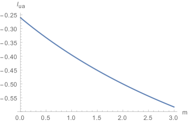
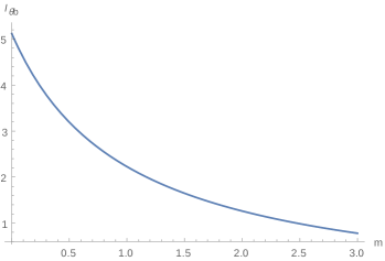
Fig. 5 shows the plots of the integrals $I_{ua}$ and $I_{tb}$ as functions of $m$. Clearly, they are perfectly well-behaved functions in our range of interest for $m$. The residues thus can be read off from these functions at the desired value of $m$. We also note that overall coefficients vanish at $d-m=1$, again indicating that there is no fermion self-energy correction at two-loop order for $d=3$ and $m=2$.

Appendix B Computation of the Feynman diagrams at three-loop level

Since the number of diagrams increases dramatically at higher loops, it is extremely hard to go beyond the two-loop level systematically. Nevertheless, we will consider some three-loop diagrams which can potentially contribute to the anomalous dimension of the boson through a non-trivial correction to $Z_{3}$, given that $Z_{3}=1$ up to the two-loop order. Here we will consider both the $\lambda_{\text{cross}}>>1$ and $\lambda_{\text{cross}}<<1$ limits.

Let us first evaluate the function

$$f_{t}(l,q)=-\frac{(i\,e)^{3}\mu^{3x/2}}{N^{3/2}}\,N\int{dp}\,{\rm Tr}\{\gamma_{d-m}\,G_{0}(p+l)\,\gamma_{d-m}\,G_{0}(p+q)\,\gamma_{d-m}\,G_{0}(p)\}\,,$$ (69)

which is formed by a fermion loop with three external boson propagators. This will be useful for all our three-loop calculations. Taking the trace in Eq. (69), we obtain

$$f_{t}(l,q) = -\frac{2e^{3}\mu^{3x/2}}{\sqrt{N}}\int\frac{d{\mathbf{P}}\,dp_{d-m+2}\ldots dp_{d}}{(2\pi)^{d-2}}\,\sum_{i=1}^{4}\kappa_{i}\,,$$ (70)

where

$$\kappa_{1} = \int\frac{dp_{d-m}\,dp_{d-m+1}}{(2\pi)^{2}}\frac{\delta_{p}\,\delta_{p+q}\,\delta_{p+l}}{den_{\kappa}}\exp\left({-\frac{{{\mathbf{L}}}_{(p)}^{2}+{{\mathbf{L}}}_{(p+q)}^{2}+{{\mathbf{L}}}_{(p+l)}^{2}}{\mu\,{\tilde{k}}_{F}}}\right)\,,$$

$$\kappa_{2} = -\int\frac{dp_{d-m}\,dp_{d-m+1}}{(2\pi)^{2}}\frac{\delta_{p}\,({\mathbf{P}}+{\mathbf{Q}})\cdot({\mathbf{P}}+{\mathbf{L}})}{den_{\kappa}}\exp\left({-\frac{{{\mathbf{L}}}_{(p)}^{2}+{{\mathbf{L}}}_{(p+q)}^{2}+{{\mathbf{L}}}_{(p+l)}^{2}}{\mu\,{\tilde{k}}_{F}}}\right)\,,$$

$$\kappa_{3} = -\int\frac{dp_{d-m}\,dp_{d-m+1}}{(2\pi)^{2}}\frac{\delta_{p+q}\,({\mathbf{P}}+{\mathbf{L}})\cdot{\mathbf{P}}}{den_{\kappa}}\exp\left({-\frac{{{\mathbf{L}}}_{(p)}^{2}+{{\mathbf{L}}}_{(p+q)}^{2}+{{\mathbf{L}}}_{(p+l)}^{2}}{\mu\,{\tilde{k}}_{F}}}\right)\,,$$

$$\kappa_{4} = -\int\frac{dp_{d-m}\,dp_{d-m+1}}{(2\pi)^{2}}\frac{\delta_{p+l}\,({\mathbf{P}}+{\mathbf{Q}})\cdot{\mathbf{P}}}{den_{\kappa}}\exp\left({-\frac{{{\mathbf{L}}}_{(p)}^{2}+{{\mathbf{L}}}_{(p+q)}^{2}+{{\mathbf{L}}}_{(p+l)}^{2}}{\mu\,{\tilde{k}}_{F}}}\right)\,,$$ (71)

$$den_{\kappa} = [\,\delta_{p}^{2}+P^{2}\,]\,[\,\delta_{p+q}^{2}+({\mathbf{P}}+{\mathbf{Q}})^{2}\,]\,[\,\delta_{p+l}^{2}+({\mathbf{P}}+{\mathbf{L}})^{2}\,]\,.$$ (72)

We assume that we are in the region $\frac{|q_{d-m}|}{|{\mathbf{L}}_{(q)}|\sqrt{2k_{F}}},\frac{|{\mathbf{P}}|+|{\mathbf{P}}+{\mathbf{Q}}|}{|{\mathbf{L}}_{(q)}|\sqrt{2k_{F}}},\frac{|{\mathbf{P}}|+|{\mathbf{P}}+{\mathbf{L}}|}{|{\mathbf{L}}_{(q)}|\sqrt{2k_{F}}}<<1$ and choose the coordinate system such that ${{\mathbf{L}}}_{(q)}=(q_{d-m+1},0,0,\ldots,0)$, without any loss of generality. We then redefine some variables as:

$$x_{1}=p_{d-m}+{{\mathbf{L}}}_{(p)}^{2}\,,\qquad x_{2}=\delta_{q}+2\,p_{d-m+1}\,|{{\mathbf{L}}}_{(q)}|\,,\quad dp_{d-m}\,dp_{d-m+1}=\frac{dx_{1}\,dx_{2}}{|q_{d-m+1}|}\,,$$

so that

$$\delta_{p}=x_{1}\,,\quad\delta_{p+q}=x_{1}+x_{2}\,,\quad\delta_{p+l}=\delta_{p}+\delta_{l}+2\,p_{d-m+1}\,l_{d-m+1}+2\,{{\mathbf{u}}}_{(p)}\cdot{{\mathbf{u}}}_{(l)}=x_{1}+\frac{l_{d-m+1}}{q_{d-m+1}}x_{2}+\Delta_{t}(p,l,q)\,,$$

with

$$\Delta_{t}(p,l,q)=\delta_{l}-\frac{l_{d-m+1}}{q_{d-m+1}}\,\delta_{q}+2\,{{\mathbf{u}}}_{(p)}\cdot{{\mathbf{u}}}_{(l)}\,,\quad{{\mathbf{u}}}_{(k)}=(k_{d-m+2},\ldots,k_{d})\,.$$ (73)

Here the vector ${{\mathbf{u}}}_{(k)}$ consists of the last $(m-1)$ components of ${{\mathbf{L}}}_{(k)}$. Neglecting the exponential damping factors for $x_{2}$, we get

$$\tilde{\kappa}_{1}$$ (74)

$$\equiv\frac{1}{2\,|q_{d-m+1}|}\int\frac{dx_{1}\,dx_{2}}{(2\pi)^{2}}\frac{x_{1}\,(x_{1}+x_{2})\,\left(x_{1}+\frac{l_{d-m+1}}{q_{d-m+1}}x_{2}+\Delta_{t}(p,l,q)\right)}{\Big{\{}x_{1}^{2}+{\mathbf{P}}^{2}\Big{\}}\Big{\{}\left(x_{1}+x_{2}\right)^{2}+({\mathbf{P}}+{\mathbf{Q}})^{2}\Big{\}}\Big{\{}\left(x_{1}+\frac{l_{d-m+1}}{q_{d-m+1}}x_{2}+\Delta_{t}(p,l,q)\right)^{2}+({\mathbf{P}}+{\mathbf{L}})^{2}\Big{\}}}$$

$$=\frac{1}{4}\int\frac{dx_{1}}{2\pi}\frac{x_{1}\,\Big{[}|l_{d-m+1}|\,|{\mathbf{P}}+{\mathbf{Q}}|+|q_{d-m+1}||{\mathbf{P}}+{\mathbf{L}}|\Big{]}\,sgn\left(q_{d-m+1}\right)}{\Big{\{}x_{1}^{2}+{\mathbf{P}}^{2}\Big{\}}\Big{\{}\left(l_{d-m+1}\,x_{1}-q_{d-m+1}(x_{1}+\Delta_{t})\right)^{2}+(\,|l_{d-m+1}|\,|{\mathbf{P}}+{\mathbf{Q}}|+|q_{d-m+1}||{\mathbf{P}}+{\mathbf{L}}|\,)^{2}\Big{\}}}$$

$$=\frac{\Delta_{t}}{8\,|q_{d-m+1}|}\frac{sgn\left(l_{d-m+1}-q_{d-m+1}\right)\,sgn\left(l_{d-m+1}\right)}{\Delta_{t}^{2}+\frac{\Big{[}|l_{d-m+1}-q_{d-m+1}|\,|{\mathbf{P}}|+|l_{d-m+1}|\,|{\mathbf{P}}+{\mathbf{Q}}|+|q_{d-m+1}|\,|{\mathbf{P}}+{\mathbf{L}}|\Big{]}^{2}}{q_{d-m+1}^{2}}}\,.$$

$$\tilde{\kappa}_{2}$$

$$\equiv\frac{1}{2\,|q_{d-m+1}|}\int\frac{dx_{1}\,dx_{2}}{(2\pi)^{2}}\frac{-x_{1}\,({\mathbf{P}}+{\mathbf{Q}})\cdot({\mathbf{P}}+{\mathbf{L}})}{\Big{\{}x_{1}^{2}+{\mathbf{P}}^{2}\Big{\}}\Big{\{}\left(x_{1}+x_{2}\right)^{2}+({\mathbf{P}}+{\mathbf{Q}})^{2}\Big{\}}\Big{\{}\left(x_{1}+\frac{l_{d-m+1}}{q_{d-m+1}}x_{2}+\Delta_{t}(p,l,q)\right)^{2}+({\mathbf{P}}+{\mathbf{L}})^{2}\Big{\}}}$$

$$=\frac{1}{4\left(l_{d-m+1}-q_{d-m+1}\right)^{2}}\int\frac{dx_{1}}{2\pi}\frac{-x_{1}\,\frac{({\mathbf{P}}+{\mathbf{Q}})\cdot({\mathbf{P}}+{\mathbf{L}})}{|{\mathbf{P}}+{\mathbf{Q}}|\,|{\mathbf{P}}+{\mathbf{L}}|}\left(\,|l_{d-m+1}|\,|{\mathbf{P}}+{\mathbf{Q}}|+|q_{d-m+1}|\,|{\mathbf{P}}+{\mathbf{L}}|\,\right)}{\Big{\{}x_{1}^{2}+{\mathbf{P}}^{2}\Big{\}}\Big{[}\Big{\{}x_{1}-\frac{q_{d-m+1}\,\Delta_{t}}{\left(l_{d-m+1}-q_{d-m+1}\right)}\Big{\}}^{2}+\left(\frac{|l_{d-m+1}|\,|{\mathbf{P}}+{\mathbf{Q}}|+|q_{d-m+1}|\,|{\mathbf{P}}+{\mathbf{L}}|}{|l_{d-m+1}-q_{d-m+1}|}\right)^{2}\Big{]}}$$

$$\Rightarrow\kappa_{2}=-\frac{({\mathbf{P}}+{\mathbf{Q}})\cdot({\mathbf{P}}+{\mathbf{L}})}{|{\mathbf{P}}+{\mathbf{Q}}|\,|{\mathbf{P}}+{\mathbf{L}}|}\,\frac{sgn\left(q_{d-m+1}\right)}{sgn\left(l_{d-m+1}\right)}\,\kappa_{1}\,.$$ (75)

$$\tilde{\kappa}_{3}$$

$$\equiv\frac{1}{2\,|q_{d-m+1}|}\int\frac{dx_{1}\,dx_{2}}{(2\pi)^{2}}\frac{-(x_{2}+x_{1})\,({\mathbf{P}}+{\mathbf{L}})\cdot{\mathbf{P}}}{\Big{\{}x_{1}^{2}+{\mathbf{P}}^{2}\Big{\}}\Big{\{}\left(x_{1}+x_{2}\right)^{2}+({\mathbf{P}}+{\mathbf{Q}})^{2}\Big{\}}\Big{\{}\left(x_{1}+\frac{l_{d-m+1}}{q_{d-m+1}}x_{2}+\Delta_{t}(p,l,q)\right)^{2}+({\mathbf{P}}+{\mathbf{L}})^{2}\Big{\}}}$$

$$=\frac{-\frac{({\mathbf{P}}+{\mathbf{L}})\cdot{\mathbf{P}}}{|{\mathbf{P}}+{\mathbf{L}}|}\,sgn\left(l_{d-m+1}\right)}{8\,\left(l_{d-m+1}-q_{d-m+1}\right)^{2}}\times\,\frac{-q_{d-m+1}\,\Delta_{t}}{|{\mathbf{P}}|}\times\,\frac{1}{\frac{q_{d-m+1}^{2}}{\left(l_{d-m+1}-q_{d-m+1}\right)^{2}}\Delta_{t}^{2}+\Big{[}|{\mathbf{P}}|+\frac{|l_{d-m+1}|\,|{\mathbf{P}}+{\mathbf{Q}}|+|q_{d-m+1}|\,|{\mathbf{P}}+{\mathbf{L}}|}{|l_{d-m+1}-q_{d-m+1}|}\Big{]}^{2}}$$

$$\Rightarrow\kappa_{3}=\frac{({\mathbf{P}}+{\mathbf{L}})\cdot{\mathbf{P}}}{|{\mathbf{P}}+{\mathbf{L}}|\,|{\mathbf{P}}|}\,\frac{sgn\left(q_{d-m+1}\right)}{sgn\left(l_{d-m+1}-q_{d-m+1}\right)}\,\kappa_{1}\,.$$ (76)

$$\tilde{\kappa}_{4}$$

$$\equiv\frac{1}{2\,|q_{d-m+1}|}\int\frac{dx_{1}\,dx_{2}}{(2\pi)^{2}}\frac{-\left(x_{1}+\frac{l_{d-m+1}}{q_{d-m+1}}x_{2}+\Delta_{t}(p,l,q)\right)\,({\mathbf{P}}+{\mathbf{Q}})\cdot{\mathbf{P}}}{\Big{\{}x_{1}^{2}+{\mathbf{P}}^{2}\Big{\}}\Big{\{}\left(x_{1}+x_{2}\right)^{2}+({\mathbf{P}}+{\mathbf{Q}})^{2}\Big{\}}\Big{\{}\left(x_{1}+\frac{l_{d-m+1}}{q_{d-m+1}}x_{2}+\Delta_{t}(p,l,q)\right)^{2}+({\mathbf{P}}+{\mathbf{L}})^{2}\Big{\}}}$$

$$=\frac{sgn\left(q_{d-m+1}\right)\,\frac{({\mathbf{P}}+{\mathbf{Q}})\cdot{\mathbf{P}}}{|{\mathbf{P}}+{\mathbf{Q}}|}}{8\left(l_{d-m+1}-q_{d-m+1}\right)^{2}}\frac{-q_{d-m+1}\,\Delta_{t}}{|{\mathbf{P}}|}\frac{1}{\frac{q_{d-m+1}^{2}}{\left(l_{d-m+1}-q_{d-m+1}\right)^{2}}\Delta_{t}^{2}+\Big{[}|{\mathbf{P}}|+\frac{|l_{d-m+1}|\,|{\mathbf{P}}+{\mathbf{Q}}|+|q_{d-m+1}|\,|{\mathbf{P}}+{\mathbf{L}}|}{|l_{d-m+1}-q_{d-m+1}|}\Big{]}^{2}}$$

$$\Rightarrow\kappa_{4}=-\frac{({\mathbf{P}}+{\mathbf{Q}})\cdot{\mathbf{P}}}{|{\mathbf{P}}+{\mathbf{Q}}|\,|{\mathbf{P}}|}\,\frac{\kappa_{1}}{sgn\left(l_{d-m+1}-q_{d-m+1}\right)\,sgn\left(l_{d-m+1}\right)\,}\,.$$ (77)

For ${\mathbf{Q}}=0$,

$$\sum_{i=1}^{4}\kappa_{i}\Big{|}_{{\mathbf{Q}}=0}=\frac{\Delta_{t}}{4\,q_{d-m+1}}\frac{{\mathbf{P}}\cdot({\mathbf{P}}+{\mathbf{L}})-|{\mathbf{P}}|\,|{\mathbf{P}}+{\mathbf{L}}|}{|{\mathbf{P}}|\,|{\mathbf{P}}+{\mathbf{L}}|}\frac{\Theta\left(l_{d-m+1}\right)-\Theta\left(l_{d-m+1}-q_{d-m+1}\right)}{\Delta_{t}^{2}+\Big{[}|{\mathbf{P}}|+|{\mathbf{P}}+{\mathbf{L}}|\Big{]}^{2}}\,.$$ (78)

We now choose ${{\mathbf{u}}}_{(l)}=(l_{d-m+2},0,0,\ldots,0)$, with $l_{d-m+2}>0$, since $f_{t}(l,q)$ can depend only on $|{{\mathbf{u}}}_{(l)}|$. Define $\quad x_{3}=2\,|{{\mathbf{u}}}_{(l)}|\,p_{d-m+2}\,,\,{{\mathbf{v}}}_{(k)}=(k_{d-m+3},\ldots,k_{d}),\,\tilde{\Delta}_{t}(l,q)=\delta_{l}-\frac{l_{d-m+1}}{q_{d-m+1}}\,\delta_{q}$ we get

$$\int\frac{dp_{d-m+2}}{2\pi}\tilde{\kappa}_{1}\,\exp\left({-\frac{3\,p_{d-m+2}^{2}+2\,|{{\mathbf{u}}}_{(l)}|\,p_{d-m+2}}{k_{F}}}\right)$$

$$=\frac{\,sgn\left(l_{d-m+1}-q_{d-m+1}\right)\,sgn\left(l_{d-m+1}\right)\,\exp\Big{[}\frac{2\,{\mathbf{u}}_{(l)}^{2}}{3\,k_{F}}\Big{]}}{16\,|{\mathbf{u}}_{(l)}|\,|q_{d-m+1}|}\int_{-\infty}^{\infty}\frac{dz_{3}}{2\pi}\frac{\left(z_{3}+u_{3}\right)\,\exp\left(-\frac{3z_{3}^{2}}{4}\right)}{\left(z_{3}+u_{3}\right)^{2}+y_{3}^{2}}\,,$$

where

$$u_{3}=\frac{-\frac{2}{3}|{{\mathbf{u}}}_{(l)}|^{2}+\tilde{\Delta}_{t}}{|{{\mathbf{u}}}_{(l)}|\,\sqrt{k_{F}}}\,,\quad y_{3}=\frac{1}{|{{\mathbf{u}}}_{(l)}|\,\sqrt{k_{F}}}\,\frac{|l_{d-m+1}-q_{d-m+1}|\,|{\mathbf{P}}|+|l_{d-m+1}|\,|{\mathbf{P}}+{\mathbf{Q}}|+|q_{d-m+1}|\,|{\mathbf{P}}+{\mathbf{L}}|}{|q_{d-m+1}|}\,.$$ (80)

1. In the limit $u_{3},\,y_{3}<<1$, we have

   $$\int_{-\infty}^{\infty}\frac{dz_{3}}{2\pi}\frac{\left(z_{3}+u_{3}\right)\,\exp\left(-\frac{3z_{3}^{2}}{4}\right)}{\left(z_{3}+u_{3}\right)^{2}+y_{3}^{2}}\simeq\sqrt{\frac{3}{4\,\pi}}\,u_{3}=\frac{1}{2\,|{\mathbf{u}}_{(l)}|^{2}}\frac{\tilde{\Delta}_{t}-\frac{2\,{\mathbf{u}}_{(l)}^{2}}{3}}{\sqrt{\pi\,k_{F}/3}}\,.$$ (81)

   Integrating the above over ${{\mathbf{v}}}_{(p)}$, we get

   $$\int\frac{d{{\mathbf{v}}}_{(p)}\,dp_{d-m+2}}{(2\pi)^{m-1}}\,\kappa_{1}$$

   $$=\int\frac{d{\mathbf{v}}_{(p)}\,dp_{d-m+2}}{(2\pi)^{m-1}}\,\tilde{\kappa}_{1}\,\exp\left({-\frac{3\,{\mathbf{v}}_{(p)}^{2}+3\,p_{d-m+2}^{2}+2\,|{{\mathbf{u}}}_{(l)}|\,p_{d-m+2}}{k_{F}}}\right)$$

   $$=sgn\left(l_{d-m+1}-q_{d-m+1}\right)\,sgn\left(l_{d-m+1}\right)\frac{\delta_{l}-\frac{l_{d-m+1}}{q_{d-m+1}}\,\delta_{q}-\frac{2\,{\mathbf{u}}_{(l)}^{2}}{3}}{2^{m+3}\,\pi\,|{\mathbf{u}}_{(l)}|^{2}\,|q_{d-m+1}|}\left(\sqrt{\frac{k_{F}}{3\pi}}\right)^{m-3}+\mathcal{O}\left(\frac{1}{k_{F}^{\frac{4-m}{2}}}\right)\,.$$

   Hence, as long as $m>1$,

   $$f_{t}(l,q) \propto e^{3}\,k_{F}^{\frac{m-3}{2}},\quad\mbox{for}\quad u_{3},\,y_{3}<<1\,\mbox{and}\,m>1.$$ (83)

2. In the limit $u_{3},\,y_{3}>>1$, we have

   $$\int_{-\infty}^{\infty}\frac{dz_{3}}{2\pi}\frac{\left(z_{3}+u_{3}\right)\,\exp\left(-\frac{3z_{3}^{2}}{4}\right)}{\left(z_{3}+u_{3}\right)^{2}+y_{3}^{2}}\simeq\frac{u_{3}}{u_{3}^{2}+y_{3}^{2}}\int_{-\infty}^{\infty}\frac{dz_{3}}{2\pi}\exp\left(-\frac{3z_{3}^{2}}{4}\right)=\frac{u_{3}}{u_{3}^{2}+y_{3}^{2}}\,\frac{1}{\sqrt{3\,\pi}}$$ (84)

   Hence we get

   $$\int\frac{d{{\mathbf{v}}}_{(p)}\,dp_{d-m+2}}{(2\pi)^{m-1}}\,\kappa_{1}$$

   $$=\frac{\left(\sqrt{\frac{k_{F}}{3\pi}}\right)^{m-1}\,sgn\left(l_{d-m+1}-q_{d-m+1}\right)\,sgn\left(l_{d-m+1}\right)}{2^{m+2}\,|q_{d-m+1}|}$$

   $$\times\,\frac{\delta_{l}-\frac{l_{d-m+1}}{q_{d-m+1}}\,\delta_{q}-\frac{2\,{\mathbf{u}}_{(l)}^{2}}{3}}{\left(\delta_{l}-\frac{l_{d-m+1}}{q_{d-m+1}}\,\delta_{q}-\frac{2\,{\mathbf{u}}_{(l)}^{2}}{3}\right)^{2}+\frac{\Big{[}|l_{d-m+1}-q_{d-m+1}|\,|{\mathbf{P}}|+|l_{d-m+1}|\,|{\mathbf{P}}+{\mathbf{Q}}|+|q_{d-m+1}|\,|{\mathbf{P}}+{\mathbf{L}}|\Big{]}^{2}}{q_{d-m+1}^{2}}}+\,\mathcal{O}\left(\frac{1}{k_{F}^{\frac{2-m}{2}}}\right)\,.$$

   Hence,

   $$f_{t}(l,q)\propto e^{3}\,k_{F}^{\frac{m-1}{2}},\quad\mbox{for}\,u_{3},\,y_{3}>>1\,.$$ (86)

   This also corresponds to the case of $m=1$. The case of $m=1$ has of course been discussed thoroughly in Dalidovich and Lee (2013).

For simplicity, we have shown the final expressions for $\kappa_{1}$ only in the appropriate limits.

B.1 Three-loop fermion self-energy diagrams with one fermion loop

(a)

(b)

(c)

Figure 6: Three-loop fermion self-energy diagrams each with one fermion loop.

Fig. 6 shows three-loop fermion self-energy diagrams each containing one fermion loop. From the computation of Fig. 2(a), it is clear that Fig. 6(c) does not contribute for $m>1$. Hence we calculate the contribution coming from the diagrams in Figs. 6(a) and  6(b). The integrals involve the function $f_{t}(l,q)$ coming from the fermion loop. Their total contribution can be written as

$$\Sigma_{3}(k) \sim \frac{(i\,e)^{3}\,\mu^{3x/2}}{N^{3/2}}\int{dq\,dl}\,\{f_{t}(l,q)+f_{t}(q-l,q)\}$$ (87)

$$\qquad\qquad\qquad\times\,\,D_{1}(l-q)\,D_{1}(q)\,D_{1}(l)\,\gamma_{d-m}\,G_{0}(k+l-q)\,\gamma_{d-m}\,G_{0}(k+l)\,\gamma_{d-m}$$

$$= \frac{i\,e^{3}\,\mu^{3x/2}}{N^{3/2}}\int dq\,dl\,\big{\{}f_{t}(l,q)+f_{t}(q-l,q)\big{\}}\,D_{1}(l-q)\,D_{1}(q)\,D_{1}(l)\,\frac{num_{30}}{den_{30}}\,,$$

where

$$num_{30} = \Big{[}\{\,{\mathbf{\Gamma}}\cdot{\mathbf{Q}}\,\}\,\{\,{\mathbf{\Gamma}}\cdot\left(\,{\mathbf{K}}\,+\,{\mathbf{L}}\,\right)\,\}\,-\,\left(\,{\mathbf{K}}\,+\,{\mathbf{L}}\,\right)^{2}\,+\,\delta_{k+l}\,\delta_{k+l-\,q}\,\Big{]}\,\gamma_{d-m}$$

$$+\,\Big{[}\{\,{\mathbf{\Gamma}}\cdot{\mathbf{Q}}\,\}\,-\,\{\,{\mathbf{\Gamma}}\cdot\left(\,{\mathbf{K}}\,+\,{\mathbf{L}}\,\right)\,\}\,\Big{]}\,\delta_{k+l}-\,\{\,{\mathbf{\Gamma}}\cdot\left(\,{\mathbf{K}}\,+\,{\mathbf{L}}\,\right)\,\}\,\delta_{k+l-q}\,,$$

$$den_{30} = \Big{[}\,\delta_{k+l}^{2}+\left(\,{\mathbf{K}}\,+\,{\mathbf{L}}\,\right)^{2}\Big{]}\,\Big{[}\,\delta_{k+l-q}^{2}+\left(\,{\mathbf{K}}\,+\,{\mathbf{L}}\,-\,{\mathbf{Q}}\,\right)^{2}\Big{]}\,,$$ (88)

and $f_{t}(l,q)$ is obtained by using Eq. (116) for $m>1$ or Eq. (2) for $m=1$. However, we must use these formulas with ${\mathbf{u}}_{l}^{2}={\mathbf{L}}_{(l)}^{2}-\frac{\left({\mathbf{L}}_{(q)}\cdot{\mathbf{L}}_{(l)}\right)^{2}}{{\mathbf{L}}_{(q)}^{2}}$ and $l_{d-m+1}=\frac{{\mathbf{L}}_{(q)}\cdot{\mathbf{L}}_{(l)}}{|{\mathbf{L}}_{(q)}|}$. Let $\theta_{ql}$ be the angle between ${\mathbf{L}}_{(q)}$ and ${\mathbf{L}}_{(l)}$. Then we can write $|{\mathbf{L}}_{(q)}|$, $|{\mathbf{L}}_{(l)}|\,\cos\theta_{ql}$ and $|{\mathbf{L}}_{(l)}|\,\sin\theta_{ql}$ in place of $q_{d-m+1}$, $l_{d-m+1}$ and $|{\mathbf{u}}_{(l)}|$ respectively.

We redefine the variables as:

$$y_{1}=\delta_{k+l}\,,\quad y_{2}=\delta_{-q}-2\,{\mathbf{L}}_{(q)}\cdot{\mathbf{L}}_{(k+l)}\,,$$ (89)

so that

$$\delta_{k+l-q}=y_{1}+y_{2}\,,\quad\delta_{q}=2\,{\mathbf{L}}_{(q)}^{2}-y_{2}-2\,{\mathbf{L}}_{(q)}\cdot{\mathbf{L}}_{(k+l)}\,,\quad\delta_{l}=y_{1}-\delta_{k}-2\,{\mathbf{L}}_{(k)}\cdot{\mathbf{L}}_{(l)}\,.$$ (90)

Using Eq. (116), which is possible for $m>1$, we have:

$$\int_{-\infty}^{\infty}\frac{d{{\mathbf{v}}}_{(p)}\,dp_{d-m+2}}{(2\pi)^{m-1}}\,\{\kappa_{1}(l,q)+\kappa_{1}(q-l,q)\}$$

$$\simeq\frac{\frac{1}{{\mathbf{u}}_{(l)}^{2}}\left(\delta_{l}-\frac{|{\mathbf{L}}_{(l)}|\,\cos\theta_{ql}}{|{\mathbf{L}}_{(q)}|}\,\delta_{q}-\frac{2\,{\mathbf{u}}_{(l)}^{2}}{3}\right)+\frac{1}{{\mathbf{u}}_{(q-l)}^{2}}\left(\delta_{q-l}-\frac{|{\mathbf{L}}_{(q)}|-|{\mathbf{L}}_{(l)}|\,\cos\theta_{ql}}{|{\mathbf{L}}_{(q)}|}\,\delta_{q}-\frac{2\,{\mathbf{u}}_{(l)}^{2}}{3}\right)}{2^{m+3}\,\pi\,|{\mathbf{L}}_{(q)}|}$$

$$\quad\times\,\left(\sqrt{\frac{k_{F}}{3\pi}}\right)^{m-3}sgn\left(|{\mathbf{L}}_{(l)}|\,\cos\theta_{ql}\right)\,sgn\left(|{\mathbf{L}}_{(q)}|-|{\mathbf{L}}_{(l)}|\,\cos\theta_{ql}\right)$$

$$= \frac{\left(\frac{k_{F}}{3\pi}\right)^{\frac{m-3}{2}}}{2^{m+3}\,\pi}sgn\left(|{\mathbf{L}}_{(l)}|\,\cos\theta_{ql}\right)\,sgn\left(|{\mathbf{L}}_{(q)}|-|{\mathbf{L}}_{(l)}|\,\cos\theta_{ql}\right)\frac{\frac{\tilde{t}_{1}}{{\mathbf{u}}_{(l)}^{2}}+\frac{\tilde{t}_{2}}{{\mathbf{u}}_{(q-l)}^{2}}}{|{\mathbf{L}}_{(q)}|}\,,$$

where

$$\tilde{t}_{1}=y_{1}+\frac{{\mathbf{L}}_{(q)}\cdot{\mathbf{L}}_{(l)}}{{\mathbf{L}}_{(q)}^{2}}\,y_{2}-\delta_{k}-2\,{\mathbf{L}}_{(k)}\cdot{\mathbf{L}}_{(l)}-\frac{2\,{\mathbf{u}}_{(l)}^{2}}{3}+2\left({\mathbf{L}}_{(q)}\cdot{\mathbf{L}}_{(l)}\right)\left(\frac{{\mathbf{L}}_{(q)}\cdot{\mathbf{L}}_{(k+l)}}{{\mathbf{L}}_{(q)}^{2}}-1\right)\,,$$

$$\tilde{t}_{2}=-\left(y_{1}+\frac{{\mathbf{L}}_{(q)}\cdot{\mathbf{L}}_{(l)}}{{\mathbf{L}}_{(q)}^{2}}\,y_{2}-\delta_{k}\right)-\frac{2\,{\mathbf{u}}_{(l)}^{2}}{3}+2\,{\mathbf{L}}_{(l)}^{2}\,.$$ (92)

There will be similar terms for the other $\kappa_{i}$’s.

One can find out the $e$ and $k_{F}$ dependence of the final answer by solving the following integrals, which appear for the various terms of the complete integrand:

$$I_{1\Sigma}=\int{dy_{1}\,dy_{2}}\,\frac{1}{\Big{[}\,y_{1}^{2}+A^{2}\Big{]}\,\Big{[}\left(y_{1}+y_{2}\right)^{2}+B^{2}\Big{]}}=\frac{\pi^{2}}{|A|\,|B|}\,.$$ (93)

$$I_{2\Sigma}=\int{dy_{1}\,dy_{2}}\,\frac{y_{1}}{\Big{[}\,y_{1}^{2}+A^{2}\Big{]}\,\Big{[}\left(y_{1}+y_{2}\right)^{2}+B^{2}\Big{]}}=0\,.$$ (94)

$$I_{3\Sigma}=\int{dy_{1}\,dy_{2}}\,\frac{y_{1}+y_{2}}{\Big{[}\,y_{1}^{2}+A^{2}\Big{]}\,\Big{[}\left(y_{1}+y_{2}\right)^{2}+B^{2}\Big{]}}=0\,.$$ (95)

$$I_{4\Sigma}=\int{dy_{1}\,dy_{2}}\,\frac{y_{1}\,\left(y_{1}+y_{2}\right)}{\Big{[}\,y_{1}^{2}+A^{2}\Big{]}\,\Big{[}\left(y_{1}+y_{2}\right)^{2}+B^{2}\Big{]}}=\pi^{2}\,.$$ (96)

$$I_{11\Sigma}=\int{dy_{1}\,dy_{2}}\,\frac{y_{1}+\frac{|{\mathbf{L}}_{(q)}\cdot{\mathbf{L}}_{(l)}|}{{\mathbf{L}}_{(q)}^{2}}\,y_{2}}{\Big{[}\,y_{1}^{2}+A^{2}\Big{]}\,\Big{[}\left(y_{1}+y_{2}\right)^{2}+B^{2}\Big{]}}=0\,.$$ (97)

$$I_{21\Sigma}=\int{dy_{1}\,dy_{2}}\,\frac{y_{1}\,\left(y_{1}+\frac{|{\mathbf{L}}_{(q)}\cdot{\mathbf{L}}_{(l)}|}{{\mathbf{L}}_{(q)}^{2}}\,y_{2}\right)}{\Big{[}\,y_{1}^{2}+A^{2}\Big{]}\,\Big{[}\left(y_{1}+y_{2}\right)^{2}+B^{2}\Big{]}}=g_{1}\left(A,B,\frac{|{\mathbf{L}}_{(q)}\cdot{\mathbf{L}}_{(l)}|}{{\mathbf{L}}_{(q)}^{2}}\right)\,.$$ (98)

$$I_{31\Sigma}=\int{dy_{1}\,dy_{2}}\,\frac{\left(y_{1}+y_{2}\right)\,\left(y_{1}+\frac{|{\mathbf{L}}_{(q)}\cdot{\mathbf{L}}_{(l)}|}{{\mathbf{L}}_{(q)}^{2}}\,y_{2}\right)}{\Big{[}\,y_{1}^{2}+A^{2}\Big{]}\,\Big{[}\left(y_{1}+y_{2}\right)^{2}+B^{2}\Big{]}}=g_{2}\left(A,B,\frac{|{\mathbf{L}}_{(q)}\cdot{\mathbf{L}}_{(l)}|}{{\mathbf{L}}_{(q)}^{2}}\right)\,.$$ (99)

$$I_{41\Sigma}=\int{dy_{1}\,dy_{2}}\,\frac{y_{1}\,\left(y_{1}+y_{2}\right)\,\left(y_{1}+\frac{|{\mathbf{L}}_{(q)}\cdot{\mathbf{L}}_{(l)}|}{{\mathbf{L}}_{(q)}^{2}}\,y_{2}\right)}{\Big{[}\,y_{1}^{2}+A^{2}\Big{]}\,\Big{[}\left(y_{1}+y_{2}\right)^{2}+B^{2}\Big{]}}=0\,.$$ (100)

To calculate the overall powers of $\tilde{e}$, $k_{F}$ and $\Lambda$, we scale out $\tilde{\alpha}$ appearing in the boson propagators by redefining variables as:

$${\mathbf{L}}_{(q)}=\left(\tilde{\alpha}\,|{\mathbf{P}}|^{d-m}\right)^{\frac{1}{3}}\,\tilde{{\mathbf{L}}}_{(q)}\,,\quad{\mathbf{L}}_{(l)}=\left(\tilde{\alpha}\,|{\mathbf{P}}|^{d-m}\right)^{\frac{1}{3}}\,\,\tilde{{\mathbf{L}}}_{(l)}\,.$$ (101)

Then we have terms proportional to:

$$\left(\frac{\tilde{e}\,\Lambda}{k_{F}}\right)^{\frac{2\,m}{m+1}}\delta_{k}=\left(\frac{\tilde{e}}{\lambda_{\text{cross}}^{\frac{1}{m+1}}}\right)^{\frac{2\,m}{m-1}}\delta_{k}\,,\quad\left(\frac{\tilde{e}\,\Lambda}{k_{F}}\right)^{\frac{2\,m}{m+1}}i\,\left({\mathbf{\Gamma}}\cdot{\mathbf{K}}\right)\sim\frac{\Lambda}{k_{F}}\,\Sigma_{2b}=\left(\frac{\tilde{e}^{2}}{\lambda_{\text{cross}}}\right)^{\frac{1}{m-1}}\,\Sigma_{2b}\,,$$

$$\frac{\tilde{e}^{2}\,\Lambda}{k_{F}}\,\delta_{k}=\left(\frac{\tilde{e}^{2\,m}}{\lambda_{\text{cross}}}\right)^{\frac{1}{m-1}}\delta_{k}\,,\quad\frac{\tilde{e}^{2}\,\Lambda}{k_{F}}\,i\,\left({\mathbf{\Gamma}}\cdot{\mathbf{K}}\right)\sim\left(\frac{\tilde{e}\,\Lambda}{k_{F}}\right)^{\frac{2\,m}{m+1}}\Sigma_{2b}=\left(\frac{\tilde{e}}{\lambda_{\text{cross}}^{\frac{1}{m+1}}}\right)^{\frac{2\,m}{m-1}}\Sigma_{2b}\,,$$ (102)

to leading order in $k$, for $m>1$. There will be similar terms for the other $\kappa_{i}$’s. Hence we conclude that for $m>1$, the three-loop terms are suppressed compared to the the one-loop terms for $\lambda_{\text{cross}}>>1$.

For $\lambda_{\text{cross}}<<1$, which includes the case of $m=1$, we have:

$$\int\frac{d{{\mathbf{v}}}_{(p)}\,dp_{d-m+2}}{(2\pi)^{m-1}}\,\{\kappa_{1}(l,q)+\kappa_{1}(-l,-q)\}$$

$$=\frac{\left(\sqrt{\frac{k_{F}}{3\pi}}\right)^{m-1}\,sgn\left(|{\mathbf{L}}_{(l)}|\,\cos\theta_{ql}-|{\mathbf{L}}_{(q)}|\right)\,sgn\left(|{\mathbf{L}}_{(l)}|\,\cos\theta_{ql}\right)}{2^{m+2}\,|{\mathbf{L}}_{(q)}|}\,\left(\frac{\tilde{t}_{1}}{\tilde{t}_{1}^{2}+\tilde{p}^{2}}+\frac{\tilde{t}_{2}}{\tilde{t}_{2}^{2}+\tilde{p}^{2}}\right)\,,$$

where $\tilde{t}_{1,2}$ has been defined in Eq. (B.1) and

$$\tilde{p}=\frac{|\,|{\mathbf{L}}_{(l)}|\,\cos\theta_{ql}-|{\mathbf{L}}_{(q)}|\,|\times\,\,|{\mathbf{P}}|+|{\mathbf{L}}_{(l)}|\,|\cos\theta_{ql}|\,|{\mathbf{P}}+{\mathbf{Q}}|+|{\mathbf{L}}_{(q)}|\,|{\mathbf{P}}+{\mathbf{L}}|}{|{\mathbf{L}}_{(q)}|}\,.$$ (104)

For the term proportional to $\gamma_{d-m}$, we need integrals of the following form:

$$I_{5\Sigma} = \int\frac{dy_{1}\,dy_{2}}{(2\,\pi)^{2}}\frac{1}{\Big{[}\,y_{1}^{2}+|{\mathbf{K}}+{\mathbf{L}}|^{2}\Big{]}\,\Big{[}\left(y_{1}+y_{2}\right)^{2}+|{\mathbf{K}}+{\mathbf{L}}-{\mathbf{Q}}|^{2}\Big{]}}\,\frac{y_{1}+\frac{l_{d-m+1}}{q_{d-m+1}}\,y_{2}-\tilde{a}}{\left(y_{1}+\frac{l_{d-m+1}}{q_{d-m+1}}\,y_{2}-\tilde{a}\right)^{2}+\tilde{p}^{2}}$$ (105)

$$= \frac{q_{d-m+1}}{l_{d-m+1}}\int\frac{dy_{1}\,dy_{2}}{(2\,\pi)^{2}}\frac{1}{\Big{[}\,y_{1}^{2}+|{\mathbf{K}}+{\mathbf{L}}|^{2}\Big{]}\,\Big{[}\left(y_{2}+y_{1}\right)^{2}+|{\mathbf{K}}+{\mathbf{L}}-{\mathbf{Q}}|^{2}\Big{]}}\,\frac{y_{2}+\frac{q_{d-m+1}}{l_{d-m+1}}\left(y_{1}-\tilde{a}\right)}{\{y_{2}+\frac{q_{d-m+1}}{l_{d-m+1}}\left(y_{1}-\tilde{a}\right)\}^{2}+\frac{q_{d-m+1}^{2}}{l_{d-m+1}^{2}}\,\tilde{p}^{2}}$$

$$= \frac{q_{d-m+1}}{2\,l_{d-m+1}\,|{\mathbf{K}}+{\mathbf{L}}-{\mathbf{Q}}|}$$

$$\times\,\int\frac{dy_{1}}{2\,\pi}\frac{\frac{q_{d-m+1}}{l_{d-m+1}}\left(y_{1}-\tilde{a}\right)-y_{1}}{\Big{[}\,y_{1}^{2}+|{\mathbf{K}}+{\mathbf{L}}|^{2}\Big{]}\,\Big{[}\{\,\frac{q_{d-m+1}}{l_{d-m+1}}\left(y_{1}-\tilde{a}\right)-y_{1}\}^{2}+\{\,|\frac{q_{d-m+1}}{l_{d-m+1}}|\,\tilde{p}+|{\mathbf{K}}+{\mathbf{L}}-{\mathbf{Q}}|\,\}^{2}\Big{]}}$$

$$= \frac{q_{d-m+1}}{2\,\left(q_{d-m+1}-l_{d-m+1}\right)\,|{\mathbf{K}}+{\mathbf{L}}-{\mathbf{Q}}|}$$

$$\times\,\int\frac{dy_{1}}{2\,\pi}\frac{y_{1}-\frac{q_{d-m+1}}{q_{d-m+1}-l_{d-m+1}}\,\tilde{a}}{\Big{[}\,y_{1}^{2}+|{\mathbf{K}}+{\mathbf{L}}|^{2}\Big{]}\,\Big{[}\{\,y_{1}-\frac{q_{d-m+1}}{q_{d-m+1}-l_{d-m+1}}\,\tilde{a}\,\}^{2}+\{\,\frac{|q_{d-m+1}|\,\tilde{p}+|l_{d-m+1}|\,|{\mathbf{K}}+{\mathbf{L}}-{\mathbf{Q}}|}{|q_{d-m+1}-l_{d-m+1}|}\,\}^{2}\Big{]}}$$

$$= \frac{-\tilde{a}}{4\,|{\mathbf{K}}+{\mathbf{L}}|\,|{\mathbf{K}}+{\mathbf{L}}-{\mathbf{Q}}|\,\Big{[}\tilde{a}^{2}+\,\{\,|1-\frac{l_{d-m+1}}{q_{d-m+1}}|\,|{\mathbf{K}}+{\mathbf{L}}|+|\frac{l_{d-m+1}}{q_{d-m+1}}|\,|{\mathbf{K}}+{\mathbf{L}}-{\mathbf{Q}}|+\tilde{p}\,\}^{2}\Big{]}}\,,$$

and

$$I_{6\Sigma} = \int\frac{dy_{1}\,dy_{2}}{(2\,\pi)^{2}}\frac{y_{1}\left(y_{1}+y_{2}\right)}{\Big{[}\,y_{1}^{2}+|{\mathbf{K}}+{\mathbf{L}}|^{2}\Big{]}\,\Big{[}\left(y_{1}+y_{2}\right)^{2}+|{\mathbf{K}}+{\mathbf{L}}-{\mathbf{Q}}|^{2}\Big{]}}\,\frac{y_{1}+\frac{l_{d-m+1}}{q_{d-m+1}}\,y_{2}-\tilde{a}}{\left(y_{1}+\frac{l_{d-m+1}}{q_{d-m+1}}\,y_{2}-\tilde{a}\right)^{2}+\tilde{p}^{2}}$$ (106)

$$= \frac{q_{d-m+1}}{l_{d-m+1}}\int\frac{dy_{1}\,dy_{2}}{(2\,\pi)^{2}}\frac{y_{1}\left(y_{2}+y_{1}\right)}{\Big{[}\,y_{1}^{2}+|{\mathbf{K}}+{\mathbf{L}}|^{2}\Big{]}\,\Big{[}\left(y_{2}+y_{1}\right)^{2}+|{\mathbf{K}}+{\mathbf{L}}-{\mathbf{Q}}|^{2}\Big{]}}\,\frac{y_{2}+\frac{q_{d-m+1}}{l_{d-m+1}}\left(y_{1}-\tilde{a}\right)}{\{y_{2}+\frac{q_{d-m+1}}{l_{d-m+1}}\left(y_{1}-\tilde{a}\right)\}^{2}+\frac{q_{d-m+1}^{2}}{l_{d-m+1}^{2}}\,\tilde{p}^{2}}$$

$$= \frac{q_{d-m+1}}{2\,l_{d-m+1}}\int\frac{dy_{1}}{2\,\pi}\,y_{1}\frac{|\frac{q_{d-m+1}}{l_{d-m+1}}|\,\tilde{p}+|{\mathbf{K}}+{\mathbf{L}}-{\mathbf{Q}}|}{\Big{[}\,y_{1}^{2}+|{\mathbf{K}}+{\mathbf{L}}|^{2}\Big{]}\,\Big{[}\{\,\frac{q_{d-m+1}}{l_{d-m+1}}\left(y_{1}-\tilde{a}\right)-y_{1}\}^{2}+\{\,|\frac{q_{d-m+1}}{l_{d-m+1}}|\,\tilde{p}+|{\mathbf{K}}+{\mathbf{L}}-{\mathbf{Q}}|\,\}^{2}\Big{]}}$$

$$= \frac{q_{d-m+1}\,l_{d-m+1}\,\left(|\frac{q_{d-m+1}}{l_{d-m+1}}|\,\tilde{p}+|{\mathbf{K}}+{\mathbf{L}}-{\mathbf{Q}}|\right)}{2\,\left(q_{d-m+1}-l_{d-m+1}\right)^{2}}$$

$$\times\,\int\frac{dy_{1}}{2\,\pi}\frac{y_{1}}{\Big{[}\,y_{1}^{2}+|{\mathbf{K}}+{\mathbf{L}}|^{2}\Big{]}\,\Big{[}\{\,y_{1}-\frac{q_{d-m+1}}{q_{d-m+1}-l_{d-m+1}}\,\tilde{a}\,\}^{2}+\{\,\frac{|q_{d-m+1}|\,\tilde{p}+|l_{d-m+1}|\,|{\mathbf{K}}+{\mathbf{L}}-{\mathbf{Q}}|}{|q_{d-m+1}-l_{d-m+1}|}\,\}^{2}\Big{]}}$$

$$= \frac{-\tilde{a}\,sgn\left(l_{d-m+1}-q_{d-m+1}\right)\,sgn\left(l_{d-m+1}\right)}{4\,\Big{[}\tilde{a}^{2}+\,\{\,|1-\frac{l_{d-m+1}}{q_{d-m+1}}|\,|{\mathbf{K}}+{\mathbf{L}}|+|\frac{l_{d-m+1}}{q_{d-m+1}}|\,|{\mathbf{K}}+{\mathbf{L}}-{\mathbf{Q}}|+\tilde{p}\,\}^{2}\Big{]}}\,.$$

Setting ${\mathbf{K}}={\mathbf{L}}_{(k)}=0$, we have then terms as:

$$\frac{\delta_{k}+\sum\limits_{\begin{subarray}{c}s_{1},s_{2}=q,l\\ j=1,\ldots,m\end{subarray}}c_{s_{1}s_{2}\,j}\,L_{(s_{1})}^{j}\,L_{(s_{2})}^{j}}{\left(\delta_{k}+\sum\limits_{\begin{subarray}{c}s_{1},s_{2}=q,l\\ j=1,\ldots,m\end{subarray}}c_{s_{1}s_{2}\,j}\,L_{(s_{1})}^{j}\,L_{(s_{2})}^{j}\right)^{2}+\{\,|1-\frac{|{\mathbf{L}}_{l}|\,\cos\theta_{ql}}{|{\mathbf{L}}_{q}|}|\,|{\mathbf{L}}|+\frac{|{\mathbf{L}}_{l}|\,|\cos\theta_{ql}|}{|{\mathbf{L}}_{q}|}\,|{\mathbf{L}}-{\mathbf{Q}}|+\tilde{p}\,\}^{2}}$$

$$+\frac{-\delta_{k}+\sum\limits_{\begin{subarray}{c}s_{1},s_{2}=q,l\\ j=1,\ldots,m\end{subarray}}\tilde{c}_{s_{1}s_{2}\,j}\,L_{(s_{1})}^{j}\,L_{(s_{2})}^{j}}{\left(-\delta_{k}+\sum\limits_{\begin{subarray}{c}s_{1},s_{2}=q,l\\ j=1,\ldots,m\end{subarray}}\tilde{c}_{s_{1}s_{2}\,j}\,L_{(s_{1})}^{j}\,L_{(s_{2})}^{j}\right)^{2}+\{\,|1-\frac{|{\mathbf{L}}_{l}|\,\cos\theta_{ql}}{|{\mathbf{L}}_{q}|}|\,|{\mathbf{L}}|+\frac{|{\mathbf{L}}_{l}|\,|\cos\theta_{ql}|}{|{\mathbf{L}}_{q}|}\,|{\mathbf{L}}-{\mathbf{Q}}|+\tilde{p}\,\}^{2}}\,.$$ (107)

We can expand to leading order in $\delta_{k}$. Furthermore, in the limit $\lambda_{\text{cross}}<<1$, the main contribution to the integral over ${\mathbf{L}}_{(q)}$ and ${\mathbf{L}}_{(l)}$ will come from $|L_{(q)}^{j}|,|L_{(l)}^{j^{\prime}}|\sim\tilde{\alpha}^{1/3}\Lambda^{\frac{d-m}{3}}<<\Lambda$. So, we can also expand in small $c_{s_{1}s_{2}\,j}\,L_{(q)}^{j}\,L_{(l)}^{j}$ and $\tilde{c}_{s_{1}s_{2}\,j}\,L_{(q)}^{j}\,L_{(l)}^{j}$, such that the leading order term proportional to $\delta_{k}$ can be extracted, which is:

$$\frac{\delta_{k}\,\left(\sum\limits_{\begin{subarray}{c}s_{1},s_{2}=q,l\\ j=1,\ldots,m\end{subarray}}\tilde{d}_{abj}\,L_{(s_{1})}^{j}\,L_{(s_{2})}^{j}\right)^{2}}{\{\,|1-\frac{|{\mathbf{L}}_{l}|\,\cos\theta_{ql}}{|{\mathbf{L}}_{q}|}|\,|{\mathbf{L}}|+\frac{|{\mathbf{L}}_{l}|\,|\cos\theta_{ql}|}{|{\mathbf{L}}_{q}|}\,|{\mathbf{L}}-{\mathbf{Q}}|+\tilde{p}\,\}^{4}}\,.$$ (108)

For the term proportional to ${\mathbf{\Gamma}}\cdot{\mathbf{K}}$, we need the following integrals:

$$I_{7\Sigma} = \int\frac{dy_{1}\,dy_{2}}{(2\,\pi)^{2}}\frac{y_{1}}{\Big{[}\,y_{1}^{2}+|{\mathbf{K}}+{\mathbf{L}}|^{2}\Big{]}\,\Big{[}\left(y_{1}+y_{2}\right)^{2}+|{\mathbf{K}}+{\mathbf{L}}-{\mathbf{Q}}|^{2}\Big{]}}\,\frac{y_{1}+\frac{l_{d-m+1}}{q_{d-m+1}}\,y_{2}-\tilde{a}}{\left(y_{1}+\frac{l_{d-m+1}}{q_{d-m+1}}\,y_{2}-\tilde{a}\right)^{2}+\tilde{p}^{2}}$$

$$= \frac{-\,sgn\left(l_{d-m+1}-q_{d-m+1}\right)\,sgn\left(l_{d-m+1}\right)\,\left(|1-\frac{l_{d-m+1}}{q_{d-m+1}}|\,|{\mathbf{K}}+{\mathbf{L}}|+|\frac{l_{d-m+1}}{q_{d-m+1}}|\,|{\mathbf{K}}+{\mathbf{L}}-{\mathbf{Q}}|+\tilde{p}\right)}{4\,|{\mathbf{K}}+{\mathbf{L}}-{\mathbf{Q}}|\,\Big{[}\tilde{a}^{2}+\,\{\,|1-\frac{l_{d-m+1}}{q_{d-m+1}}|\,|{\mathbf{K}}+{\mathbf{L}}|+|\frac{l_{d-m+1}}{q_{d-m+1}}|\,|{\mathbf{K}}+{\mathbf{L}}-{\mathbf{Q}}|+\tilde{p}\,\}^{2}\Big{]}}\,,$$

and

$$I_{8\Sigma} = \int\frac{dy_{1}\,dy_{2}}{(2\,\pi)^{2}}\frac{\left(y_{1}+y_{2}\right)}{\Big{[}\,y_{1}^{2}+|{\mathbf{K}}+{\mathbf{L}}|^{2}\Big{]}\,\Big{[}\left(y_{1}+y_{2}\right)^{2}+|{\mathbf{K}}+{\mathbf{L}}-{\mathbf{Q}}|^{2}\Big{]}}\,\frac{y_{1}+\frac{l_{d-m+1}}{q_{d-m+1}}\,y_{2}-\tilde{a}}{\left(y_{1}+\frac{l_{d-m+1}}{q_{d-m+1}}\,y_{2}-\tilde{a}\right)^{2}+\tilde{p}^{2}}$$ (110)

$$= \frac{\,sgn\left(q_{d-m+1}\right)\,sgn\left(l_{d-m+1}\right)\,\{\,|1-\frac{l_{d-m+1}}{q_{d-m+1}}|\,|{\mathbf{K}}+{\mathbf{L}}|+|\frac{l_{d-m+1}}{q_{d-m+1}}|\,|{\mathbf{K}}+{\mathbf{L}}-{\mathbf{Q}}|+\tilde{p}\,\}}{4\,|{\mathbf{K}}+{\mathbf{L}}|\,\Big{[}\tilde{a}^{2}+\,\{\,|1-\frac{l_{d-m+1}}{q_{d-m+1}}|\,|{\mathbf{K}}+{\mathbf{L}}|+|\frac{l_{d-m+1}}{q_{d-m+1}}|\,|{\mathbf{K}}+{\mathbf{L}}-{\mathbf{Q}}|+\tilde{p}\,\}^{2}\Big{]}}\,.$$

Setting $\delta_{k}={\mathbf{L}}_{(k)}=0$, now we have terms as:

$$\frac{1}{\left(\sum\limits_{\begin{subarray}{c}s_{1},s_{2}=q,l\\ j=1,\ldots,m\end{subarray}}c_{s_{1}s_{2}\,j}\,L_{(s_{1})}^{j}\,L_{(s_{2})}^{j}\right)^{2}+\{\,|1-\frac{|{\mathbf{L}}_{l}|\,\cos\theta_{ql}}{|{\mathbf{L}}_{q}|}|\,|{\mathbf{L}}|+\frac{|{\mathbf{L}}_{l}|\,|\cos\theta_{ql}|}{|{\mathbf{L}}_{q}|}\,|{\mathbf{L}}-{\mathbf{Q}}|+\tilde{p}\,\}^{2}}$$

$$+\frac{1}{\left(\sum\limits_{\begin{subarray}{c}s_{1},s_{2}=q,l\\ j=1,\ldots,m\end{subarray}}\tilde{c}_{s_{1}s_{2}\,j}\,L_{(s_{1})}^{j}\,L_{(s_{2})}^{j}\right)^{2}+\{\,|1-\frac{|{\mathbf{L}}_{l}|\,\cos\theta_{ql}}{|{\mathbf{L}}_{q}|}|\,|{\mathbf{L}}|+\frac{|{\mathbf{L}}_{l}|\,|\cos\theta_{ql}|}{|{\mathbf{L}}_{q}|}\,|{\mathbf{L}}-{\mathbf{Q}}|+\tilde{p}\,\}^{2}}\,,$$ (111)

which can be expanded to leading order in small $c_{s_{1}s_{2}\,j}\,L_{(q)}^{j}\,L_{(l)}^{j}$ and $\tilde{c}_{s_{1}s_{2}\,j}\,L_{(q)}^{j}\,L_{(l)}^{j}$. The leading order term proportional to ${\mathbf{\Gamma}}\cdot{\mathbf{K}}$ can now be extracted, which is:

$$\frac{{\mathbf{\Gamma}}\cdot{\mathbf{K}}\,\left(\sum\limits_{\begin{subarray}{c}s_{1},s_{2}=q,l\\ j=1,\ldots,m\end{subarray}}\tilde{g}_{s_{1}s_{2}\,j}\,L_{(s_{1})}^{j}\,L_{(s_{2})}^{j}\right)^{2}}{\{\,|1-\frac{|{\mathbf{L}}_{l}|\,\cos\theta_{ql}}{|{\mathbf{L}}_{q}|}|\,|{\mathbf{L}}|+\frac{|{\mathbf{L}}_{l}|\,|\cos\theta_{ql}|}{|{\mathbf{L}}_{q}|}\,|{\mathbf{L}}-{\mathbf{Q}}|+\tilde{p}\,\}^{4}}\,.$$ (112)

Again, to calculate the overall powers of ${\tilde{e}}$, $k_{F}$ and $\Lambda$, we scale out $\tilde{\alpha}$ appearing in the boson propagators by redefining variables as:

$${\mathbf{L}}_{(q)}=\left(\tilde{\alpha}\,|{\mathbf{P}}|^{d-m}\right)^{\frac{1}{3}}\,\tilde{{\mathbf{L}}}_{(q)}\,,\quad{\mathbf{L}}_{(l)}=\left(\tilde{\alpha}\,|{\mathbf{P}}|^{d-m}\right)^{\frac{1}{3}}\,\,\tilde{{\mathbf{L}}}_{(l)}\,.$$ (113)

Then the overall dependence is

$$\Sigma_{3a}(q) \sim {\tilde{e}}^{\frac{2\,(m+3)}{m+1}}\left(\frac{k_{F}}{\Lambda}\right)^{\frac{2\,(m-1)}{m+1}}\gamma_{d-m}\,\delta_{q}={\lambda_{\text{cross}}}^{\frac{m+3}{m+1}}\left(\frac{\Lambda}{k_{F}}\right)^{m-1}\gamma_{d-m}\,\delta_{q}\,,$$

$$\Sigma_{3b}(q) \sim {\tilde{e}}^{\frac{2\,(m+3)}{m+1}}\left(\frac{k_{F}}{\Lambda}\right)^{\frac{2\,(m-1)}{m+1}}\left({\mathbf{\Gamma}}\cdot{\mathbf{Q}}\right)={\lambda_{\text{cross}}}^{\frac{m+3}{m+1}}\left(\frac{\Lambda}{k_{F}}\right)^{m-1}\left({\mathbf{\Gamma}}\cdot{\mathbf{Q}}\right).$$ (114)

This shows that there is a logarithmic divergence at $m=1$. However, for $m>1$, in the limit $\lambda_{\text{cross}}\ll 1$, the integral is not divergent, a behaviour which is also seen for the $\lambda_{\text{cross}}\gg 1$ limit.

B.2 Three-loop Aslamazov-Larkin-type contribution to boson self-energy

Figure 7: Aslamazov-Larkin type contributions to boson self-energy. Diagrams (a) and (b) correspond to the particle-particle and particle-hole channels respectively.

The Aslamazov-Larkin (AL) type diagrams shown in Fig. 7 are the lowest order diagrams that can renormalize the boson kinetic term Metlitski and Sachdev (2010a); Mross et al. (2010). These give a three-loop contribution to boson self-energy as

$$\Pi_{AL}(q)=\Pi_{pp}(q)+\Pi_{ph}(q)=\int dl\,D_{1}(l)\,D_{1}(l-q)\,f_{t}(l,q)\,[\,f_{t}(l,q)+f_{t}(-l,-q)\,]\,.$$ (115)

We will consider ${\mathbf{Q}}=0$ for simplicity, which is enough to examine the divergences. Also, the coordinate system is oriented such that ${\mathbf{L}}_{(q)}=\left(q_{d-m+1},0,\ldots,0\right)$ .

For $\lambda_{\text{cross}}>>1$, we have

$$f_{t}(l,q;{\mathbf{Q}}=0) = \frac{e^{3}\mu^{3\,x/2}}{\sqrt{N}}\int\frac{d{\mathbf{P}}}{(2\,\pi)^{d-m}}\frac{\Big{[}{\mathbf{P}}\cdot({\mathbf{P}}+{\mathbf{L}})-|{\mathbf{P}}|\,|{\mathbf{P}}+{\mathbf{L}}|\Big{]}\,\Big{[}\Theta\left(l_{d-m+1}\right)-\Theta\left(l_{d-m+1}-q_{d-m+1}\right)\Big{]}}{|{\mathbf{P}}|\,|{\mathbf{P}}+{\mathbf{L}}|}$$ (116)

$$\times\,\frac{\delta_{l}-\frac{l_{d-m+1}}{q_{d-m+1}}\,\delta_{q}-\frac{2\,{\mathbf{u}}_{(l)}^{2}}{3}}{2^{m+3}\,\pi\,|{\mathbf{u}}_{(l)}|^{2}\,q_{d-m+1}}\left(\sqrt{\frac{k_{F}}{3\pi}}\right)^{m-3}\,.$$

For $\lambda_{\text{cross}}<<1$, which includes the case $m=1$, we have

$$f_{t}(l,q;{\mathbf{Q}}=0) = \frac{e^{3}\mu^{3\,x/2}}{\sqrt{N}}\int\frac{d{\mathbf{P}}}{(2\,\pi)^{d-m}}\frac{\Big{[}{\mathbf{P}}\cdot({\mathbf{P}}+{\mathbf{L}})-|{\mathbf{P}}|\,|{\mathbf{P}}+{\mathbf{L}}|\Big{]}\,\Big{[}\Theta\left(l_{d-m+1}\right)-\Theta\left(l_{d-m+1}-q_{d-m+1}\right)\Big{]}}{|{\mathbf{P}}|\,|{\mathbf{P}}+{\mathbf{L}}|}$$ (117)

$$\qquad\qquad\times\,\frac{\left(\sqrt{\frac{k_{F}}{3\pi}}\right)^{m-1}}{2^{m+2}\,q_{d-m+1}}\frac{\delta_{l}-\frac{l_{d-m+1}}{q_{d-m+1}}\,\delta_{q}-\frac{2\,{\mathbf{u}}_{(l)}^{2}}{3}}{\left(\delta_{l}-\frac{l_{d-m+1}}{q_{d-m+1}}\,\delta_{q}-\frac{2\,{\mathbf{u}}_{(l)}^{2}}{3}\right)^{2}+\Big{[}|{\mathbf{P}}|+|{\mathbf{P}}+{\mathbf{L}}|\Big{]}^{2}}\,.$$

First, let us focus on this limit of $\lambda_{\text{cross}}<<1$ in order to see if $Z_{3}$ gets a correction from the AL terms for this range. For the particle-hole channel containing $f(l,q)\,f(l,q)$, we redefine variables as $y=\delta_{l}-\frac{l_{d-m+1}}{q_{d-m+1}}\,\delta_{q}-\frac{2\,{\mathbf{u}}_{(l)}^{2}}{3}$, and integrate over $l_{d-m}$ to obtain

$$\Pi_{ph}(q;{\mathbf{Q}}=0) = \frac{e^{6}\mu^{3\,x}}{N\,q_{d-m+1}^{2}}\int\frac{d{\mathbf{P}}\,d{\mathbf{K}}\,d{\mathbf{L}}\,d{\mathbf{L}}_{l}}{(2\pi)^{3d+1-2m}}D_{1}(l)D_{1}(l-q)\Big{[}\Theta\left(l_{d-m+1}\right)-\Theta\left(l_{d-m+1}-q_{d-m+1}\right)\Big{]}^{2}$$ (118)

$$\qquad\qquad\times\frac{\left(\,[{\mathbf{P}}\cdot({\mathbf{P}}+{\mathbf{L}})]-|{\mathbf{P}}|\,|{\mathbf{P}}+{\mathbf{L}}|\,\right)\left(\,[{\mathbf{K}}\cdot({\mathbf{K}}+{\mathbf{L}})]-|{\mathbf{K}}|\,|{\mathbf{K}}+{\mathbf{L}}|\,\right)}{8\,|{\mathbf{P}}|\,|{\mathbf{K}}|\,|{\mathbf{P}}+{\mathbf{L}}|\,|{\mathbf{K}}+{\mathbf{L}}|\left[\,|{\mathbf{P}}|+|{\mathbf{P}}+{\mathbf{L}}|+|{\mathbf{K}}|+|{\mathbf{K}}+{\mathbf{L}}|\,\right]}.$$

To calculate the contribution in the particle-particle channel containing $f(l,q)f(-l,-q)$, we define $\tilde{y}=l_{d-m}-\frac{l_{d-m+1}}{q_{d-m+1}}\,q_{d-m}$, and integrate over $l_{d-m}$ to get

$$\Pi_{pp}(q;{\mathbf{Q}}=0) = -\frac{e^{6}\mu^{3\,x}}{N\,q_{d-m+1}^{2}}\int\frac{d{\mathbf{P}}\,d{\mathbf{K}}\,d{\mathbf{L}}\,d{\mathbf{L}}_{l}}{(2\pi)^{3d+1-2m}}D_{1}(l)\,D_{1}(l-q)\Big{[}\Theta\left(l_{d-m+1}\right)-\Theta\left(l_{d-m+1}-q_{d-m+1}\right)\Big{]}^{2}$$

$$\qquad\qquad\times\,\frac{\left([{\mathbf{P}}\cdot({\mathbf{P}}+{\mathbf{L}})]-|{\mathbf{P}}|\,|{\mathbf{P}}+{\mathbf{L}}|\right)\left([{\mathbf{K}}\cdot({\mathbf{K}}+{\mathbf{L}})]-|{\mathbf{K}}|\,|{\mathbf{K}}+{\mathbf{L}}|\right)}{8\,|{\mathbf{P}}|\,|{\mathbf{K}}|\,|{\mathbf{P}}+{\mathbf{L}}|\,|{\mathbf{K}}+{\mathbf{L}}|}$$

$$\qquad\qquad\times\,\frac{|{\mathbf{P}}|+|{\mathbf{P}}+{\mathbf{L}}|+|{\mathbf{K}}|+|{\mathbf{K}}+{\mathbf{L}}|}{\left[\,|{\mathbf{P}}|+|{\mathbf{P}}+{\mathbf{L}}|+|{\mathbf{K}}|+|{\mathbf{K}}+{\mathbf{L}}|\,\right]^{2}+4\,\left(l_{d-m+1}^{2}-l_{d-m+1}\,q_{d-m+1}+\frac{{\mathbf{u}}_{(l)}^{2}}{3}\right)^{2}}$$

$$= -\frac{4\,e^{6}\mu^{3\,x}}{N\,q_{d-m+1}^{2}}\int\frac{d{\mathbf{P}}\,d{\mathbf{K}}\,d{\mathbf{L}}\,d{\mathbf{u}}_{l}}{(2\pi)^{3d+1-2m}}\int_{0}^{|q_{d-m+1}|}dl_{d-m+1}\,D_{1}(l)\,D_{1}(l-q;q_{d-m+1}\rightarrow|q_{d-m+1}|)$$

$$\qquad\qquad\times\,\frac{\left([{\mathbf{P}}\cdot({\mathbf{P}}+{\mathbf{L}})]-|{\mathbf{P}}|\,|{\mathbf{P}}+{\mathbf{L}}|\right)\left([{\mathbf{K}}\cdot({\mathbf{K}}+{\mathbf{L}})]-|{\mathbf{K}}|\,|{\mathbf{K}}+{\mathbf{L}}|\right)}{8\,|{\mathbf{P}}|\,|{\mathbf{K}}|\,|{\mathbf{P}}+{\mathbf{L}}|\,|{\mathbf{K}}+{\mathbf{L}}|}$$

$$\qquad\qquad\times\,\frac{|{\mathbf{P}}|+|{\mathbf{P}}+{\mathbf{L}}|+|{\mathbf{K}}|+|{\mathbf{K}}+{\mathbf{L}}|}{\left[\,|{\mathbf{P}}|+|{\mathbf{P}}+{\mathbf{L}}|+|{\mathbf{K}}|+|{\mathbf{K}}+{\mathbf{L}}|\,\right]^{2}+4\,\left(l_{d-m+1}^{2}-l_{d-m+1}\,|q_{d-m+1}|+\frac{{\mathbf{u}}_{(l)}^{2}}{3}\right)^{2}}\,.$$

Although $\Pi_{pp}(q)$ and $\Pi_{ph}(q)$ are individually UV divergent, their sum results in a UV finite correction. Rescaling $l_{d-m+1}$ as

$$l_{d}\rightarrow l_{d-m+1}\,|q_{d-m+1}|$$ (120)

to make the integral over $l_{d-m+1}$ run from $0$ to $1$, and rescaling

$${\mathbf{L}}\rightarrow 2\,q_{d-m+1}^{2}\,l_{d-m+1}\,(1-l_{d-m+1})\,{\mathbf{L}}\,,\,{\mathbf{P}}\rightarrow 2\,q_{d-m+1}^{2}\,l_{d-m+1}\,(1-l_{d-m+1})\,{\mathbf{P}}\,,$$

$${\mathbf{K}}\rightarrow 2\,q_{d-m+1}^{2}\,l_{d-m+1}\,(1-l_{d-m+1})\,{\mathbf{K}}\,,$$ (121)

we arrive at the expression:

$$\Pi_{AL}(q;{\mathbf{Q}}=0) = \frac{e^{6}\,\mu^{3\,x}\,|{\mathbf{L}}_{q}|^{6\,(d-m-1)-m}}{N}\int\frac{d{\mathbf{P}}d{\mathbf{K}}d{\mathbf{L}}}{(2\pi)^{3\,(d-m)}}\frac{{\cal J}_{m}(|{\mathbf{L}}|)}{\left(\,|{\mathbf{P}}|+|{\mathbf{P}}+{\mathbf{L}}|+|{\mathbf{K}}|+|{\mathbf{K}}+{\mathbf{L}}|\,\right)^{2}+1}$$ (122)

$$\cdot \frac{\left([{\mathbf{K}}\cdot({\mathbf{K}}+{\mathbf{L}})]-|{\mathbf{K}}|\,|{\mathbf{K}}+{\mathbf{L}}|\right)\,\left([{\mathbf{P}}\cdot({\mathbf{P}}+{\mathbf{L}})]-|{\mathbf{P}}|\,|{\mathbf{P}}+{\mathbf{L}}|\right)}{2\,|{\mathbf{P}}|\,|{\mathbf{K}}|\,|{\mathbf{P}}+{\mathbf{L}}|\,|{\mathbf{K}}+{\mathbf{L}}|\left[\,|{\mathbf{P}}|+|{\mathbf{P}}+{\mathbf{L}}|+|{\mathbf{K}}|+|{\mathbf{K}}+{\mathbf{L}}|\,\right]},$$

where

$${\cal J}_{m}(|{\mathbf{L}}|) \sim \int_{0}^{1}\frac{dl_{d-m+1}}{2\,\pi}\frac{2^{3d-6}\,[\,l_{d-m+1}\,(1-l_{d-m+1})\,]^{2\,(d-m)}}{l_{d-m+1}^{3-d+m}+\tilde{\alpha}\,[\,2\,(1-l_{d-m+1})\,|{\mathbf{L}}|\,]^{d-m}}\frac{1}{(1-l_{d-m+1})^{3-d+m}+\tilde{\alpha}\,\left(\,2\,l_{d-m+1}\,|{\mathbf{L}}|\,\right)^{d-m}}\,.$$

Here ${\mathbf{P}},{\mathbf{K}}$ and ${\mathbf{L}}$ have been rescaled to be dimensionless in the unit of $q_{d-m+1}^{2}$. Since ${\cal J}_{m}(|{\mathbf{L}}|)$ decays as $|{\mathbf{L}}|^{-2\,(d-m)}$ in the $|{\mathbf{L}}|\rightarrow\infty$ limit, the overall degree of divergence of the ${\mathbf{P}},{\mathbf{L}}$ and ${\mathbf{K}}$ integrals is $-3+d-m$, which is UV-finite. To estimate the dependence on $\tilde{e}$ and $k_{F}$, we note that ${\cal J}_{m}(|{\mathbf{L}}|)$ has a non-trivial dependence on $\tilde{\alpha}$, and behaves differently depending on whether $|{\mathbf{L}}|$ is large or small compared to $L_{*}=\tilde{\alpha}^{-\frac{1}{d-m}}$ (in the unit of $q_{d-m+1}^{2}$) :

$${\cal J}_{m}(L)\approx\left\{\begin{array}[]{cl}C_{1},&\quad|{\mathbf{L}}|\ll L_{*}\\ \displaystyle\frac{C_{2}}{\tilde{\alpha}^{2}\,|{\mathbf{L}}|^{2\,(d-m)}},&\quad|{\mathbf{L}}|\gg L_{*}\end{array}\right\}\,,$$ (126)

where $C_{1}$ and $C_{2}$ are constants which are independent of $\tilde{e}$ and $k_{F}$. Thus the Aslamazov-Larkin diagrams contribute only a finite renormalization to the boson kinetic term and the $m=2$ case in the $\lambda_{\text{cross}}<<1$ limit still has $Z_{3}=1$ even at this three-loop order.

For the sake of completeness, let us also enumerate the behaviour of the AL terms in some other specific limits.

For $\frac{|q_{d-m}|}{|{\mathbf{L}}_{(q)}|\sqrt{2k_{F}}},\frac{|{\mathbf{Q}}|}{|{\mathbf{L}}_{(q)}|\sqrt{2k_{F}}}<<1$:

1. For $\frac{|l_{d-m}|}{|{\mathbf{L}}_{(l)}|\sqrt{2k_{F}}},\frac{|{\mathbf{L}}|}{|{\mathbf{L}}_{(l)}|\sqrt{2k_{F}}}<<1$ and $m>1$, we use Eq. (83) to get

   $$\big{[}\mbox{Integral for }|{{\mathbf{L}}}_{(l)}|>\frac{\Lambda}{\sqrt{k_{F}}}\mbox{ contributing to }\Pi_{AL}(q)\big{]}$$

   $$\propto \frac{e^{6}\,\mu^{3x}\,k_{F}^{m-3}}{|{\mathbf{L}}_{(q)}|^{4}}\int_{|{{\mathbf{L}}}_{(l)}|>\frac{\Lambda}{\sqrt{k_{F}}}}\frac{dl}{(2\pi)^{d+1}}\frac{|{{\mathbf{L}}}_{(l)}|}{|{\mathbf{L}}_{(l)}|^{3}+\tilde{\alpha}\,|{\mathbf{L}}|^{d-m}}\frac{|{{\mathbf{L}}}_{(l-q)}|}{|{\mathbf{L}}_{(l-q)}|^{3}+\tilde{\alpha}\,|{\mathbf{L}}-{\mathbf{Q}}|^{d-m}}\times fn(q,l)\,.$$

   The positive powers of $k_{F}$ in the denominator of the boson propagator will further suppress the final expression by overall negative powers of $k_{F}$. But let us estimate the overall powers by ignoring these. Then the factors go as

   $$e^{2}\,k_{F}^{\frac{m-1}{2}}\times\frac{{\tilde{e}}^{\frac{6}{(m+1)}}}{k_{F}^{\frac{9-2m+m^{2}}{2\,(m+1)}}}\,.$$ (128)

2. In the limit $\frac{|q_{d-m}|}{|{\mathbf{L}}_{(q)}|\sqrt{2k_{F}}},\frac{|{\mathbf{P}}|+|{\mathbf{P}}+{\mathbf{Q}}|}{|{\mathbf{L}}_{(q)}|\sqrt{2k_{F}}},\frac{|{\mathbf{P}}|+|{\mathbf{P}}+{\mathbf{L}}|}{|{\mathbf{L}}_{(q)}|\sqrt{2k_{F}}}<<1$ and $\frac{|l_{d-m}|}{|{\mathbf{L}}_{(l)}|\sqrt{2k_{F}}},\frac{|{\mathbf{L}}|}{|{\mathbf{L}}_{(l)}|\sqrt{2k_{F}}}>>1$, we have

   $$\kappa_{1} \simeq \frac{1}{2\,|{{\mathbf{L}}}_{(q)}|}\int\frac{dx_{1}}{2\pi}\frac{x_{1}\,\left(x_{1}+l_{d-m}\right)\exp\left({-\frac{3{{\mathbf{u}}}_{(p)}^{2}+{{\mathbf{L}}}_{(q)}^{2}}{k_{F}}}\right)}{\Big{\{}x_{1}^{2}+{\mathbf{P}}^{2}\Big{\}}\Big{\{}\left(x_{1}+l_{d-m}\right)^{2}+({\mathbf{P}}+{\mathbf{L}})^{2}\Big{\}}}$$ (129)

   $$\times\,\int\frac{dx_{2}}{2\pi}\frac{\left(x_{1}+x_{2}+\delta_{q}\right)\exp\left({-\frac{3x_{2}^{2}\,+\,4\,{\mathbf{L}}_{(q)}^{2}\,x_{2}}{4\,{\mathbf{L}}_{(q)}^{2}\,k_{F}}}\right)}{\left(x_{1}+x_{2}+\delta_{q}\right)^{2}+({\mathbf{P}}+{\mathbf{Q}})^{2}}$$

   $$= \frac{1}{2\,|{{\mathbf{L}}}_{(q)}|}\int\frac{dx_{1}}{2\pi}\frac{x_{1}\,\left(x_{1}+l_{d-m}\right)\exp\left({-\frac{3{{\mathbf{u}}}_{(p)}^{2}+\frac{2}{3}{{\mathbf{L}}}_{(q)}^{2}}{k_{F}}}\right)}{\Big{\{}x_{1}^{2}+{\mathbf{P}}^{2}\Big{\}}\Big{\{}\left(x_{1}+l_{d-m}\right)^{2}+({\mathbf{P}}+{\mathbf{L}})^{2}\Big{\}}}$$

   $$\qquad\quad\times\,\int\frac{dx_{2}}{2\pi}\frac{\left(x_{1}+x_{2}+\delta_{q}-\frac{2}{3}{\mathbf{L}}_{(q)}^{2}\right)\exp\left({-\frac{3x_{2}^{2}}{4\,{\mathbf{L}}_{(q)}^{2}\,k_{F}}}\right)}{\left(x_{1}+x_{2}+\delta_{q}-\frac{2}{3}{\mathbf{L}}_{(q)}^{2}\right)^{2}+({\mathbf{P}}+{\mathbf{Q}})^{2}}\,.$$

   This implies that

   $$f_{t}(l,q)=\frac{e^{3}\,k_{F}^{\frac{m-2}{2}}}{2\,|{{\mathbf{L}}}_{(q)}|}\times fn({\mathbf{L}},q,l_{d-m})$$ (130)

   in these limits.

   Hence, for $\frac{|l_{d-m}|}{|{\mathbf{L}}_{(l)}|\sqrt{2k_{F}}},\frac{|{\mathbf{L}}|}{|{\mathbf{L}}_{(l)}|\sqrt{2k_{F}}}>>1$ and $m>1$, Eqs. (130) and Eq. (A15) of Ref. Mandal and Lee (2015) give us:

   $$\big{[}\mbox{Integral for }|{{\mathbf{L}}}_{(l)}|<\frac{\Lambda}{\sqrt{k_{F}}}\mbox{ contributing to }\Pi_{AL}(q)\big{]}$$

   $$\propto \frac{e^{6}\,k_{F}^{m-2}}{|{\mathbf{L}}_{(q)}|^{2}}\int_{|{{\mathbf{L}}}_{(l)}|<\frac{\Lambda}{\sqrt{k_{F}}}}\frac{dl}{(2\pi)^{d+1}}\frac{fn({\mathbf{L}},l_{d-m},q)}{{{\mathbf{L}}}_{(l)}^{2}+e^{2}\,\mu^{x}\,J^{m-1}\sqrt{k_{F}}\,\,\tilde{f}\left(|{\mathbf{L}}|,l_{d-m}\right)}\frac{|{{\mathbf{L}}}_{(q)}|}{|{\mathbf{L}}_{(q)}|^{3}+\tilde{\alpha}\,|{\mathbf{L}}-{\mathbf{Q}}|^{d-m}}$$

   $$\propto \frac{e^{4}\,\Lambda^{m}}{|{\mathbf{L}}_{(q)}|^{2}\,k_{F}^{2}}\int\frac{d{\mathbf{L}}\,dl_{d-m}}{(2\pi)^{d-m+1}}\frac{fn({\mathbf{L}},l_{d-m},q)}{|{\mathbf{L}}_{(q)}|^{3}+\tilde{\alpha}\,|{\mathbf{L}}-{\mathbf{Q}}|^{d-m}}\,.$$

   Again, ignoring the negative powers of $k_{F}$ coming from $\tilde{\alpha}$, we get the factors as

   $$e^{2}\,k_{F}^{\frac{m}{2}}\times\frac{{\tilde{e}}^{\frac{3}{(m+1)}}}{k_{F}^{\frac{m^{2}+m+3}{(m+1)}}}\,.$$ (132)

For $\frac{|q_{d-m}|}{|{\mathbf{L}}_{(q)}|\sqrt{2k_{F}}},\frac{|{\mathbf{Q}}|}{|{\mathbf{L}}_{(q)}|\sqrt{2k_{F}}}>>1$:

1. In the limit $\frac{|l_{d-m}|}{{\mathbf{L}}_{(l)}\sqrt{2k_{F}}}<<1$, we get

   $$\kappa_{1} \simeq \exp\left({-\frac{{{\mathbf{L}}}_{(q)}^{2}+{{\mathbf{L}}}_{(l)}^{2}}{3\,k_{F}}}\right)\int\frac{dx_{1}\,dp_{d-m+1}}{(2\pi)^{2}}\frac{\exp\left({-\frac{3\left({{\mathbf{L}}}_{(p)}+\frac{1}{3}{{\mathbf{L}}}_{(q)}+\frac{1}{3}{{\mathbf{L}}}_{(l)}\right)^{2}}{k_{F}}}\right)}{\Big{\{}x_{1}^{2}+{\mathbf{P}}^{2}\Big{\}}\Big{\{}\left(x_{1}+q_{d-m}\right)^{2}+({\mathbf{P}}+{\mathbf{Q}})^{2}\Big{\}}}$$

   $$\qquad\qquad\qquad\qquad\qquad\qquad\qquad\times\frac{x_{1}\,(x_{1}+q_{d-m})\,\Big{\{}x_{1}+{{\mathbf{L}}}_{(l)}^{2}+2{{\mathbf{L}}}_{(p)}\cdot{{\mathbf{L}}}_{(l)}\Big{\}}}{\Big{\{}x_{1}+{{\mathbf{L}}}_{(l)}^{2}+2{{\mathbf{L}}}_{(p)}\cdot{{\mathbf{L}}}_{(l)}\Big{\}}^{2}+({\mathbf{P}}+{\mathbf{L}})^{2}}$$

   $$\implies \int\frac{d{\mathbf{u}}_{(p)}}{(2\pi)^{m-1}}\,\kappa_{1}$$

   $$= \exp\left({-\frac{{{\mathbf{L}}}_{(q)}^{2}+{{\mathbf{L}}}_{(l)}^{2}}{3\,k_{F}}}\right)\left(\frac{k_{F}}{12\pi}\right)^{\frac{m-1}{2}}\sqrt{\frac{3}{\pi k_{F}}}\int\frac{dx_{1}}{2\pi}\frac{x_{1}\,(x_{1}+q_{d-m})\,(x_{1}+\frac{1}{3}{{\mathbf{L}}}_{(l)}^{2}-\frac{2}{3}{{\mathbf{L}}}_{(l)}\cdot{{\mathbf{L}}}_{(q)})}{\Big{\{}x_{1}^{2}+{\mathbf{P}}^{2}\Big{\}}\Big{\{}\left(x_{1}+q_{d-m}\right)^{2}+({\mathbf{P}}+{\mathbf{Q}})^{2}\Big{\}}}\,.$$

   This implies

   $$f_{t}(l,q)\propto e^{3}\,k_{F}^{\frac{m-2}{2}}$$ (134)

   in the above limits.

   Therefore, for $\frac{|l_{d-m}|}{|{\mathbf{L}}_{(l)}|\sqrt{2k_{F}}},\frac{|{\mathbf{L}}|}{|{\mathbf{L}}_{(l)}|\sqrt{2k_{F}}}<<1$ and $m>1$, we use Eq. (134) to get

   $$\big{[}\mbox{Integral for }|{{\mathbf{L}}}_{(l)}|>\frac{\Lambda}{\sqrt{k_{F}}}\mbox{ contributing to }\Pi_{AL}(q)\big{]}$$

   $$\propto e^{6}\,k_{F}^{m-2}\int_{|{{\mathbf{L}}}_{(l)}|>\frac{\Lambda}{\sqrt{k_{F}}}}\frac{dl}{(2\pi)^{d+1}}\frac{|{{\mathbf{L}}}_{(l)}|}{|{\mathbf{L}}_{(l)}|^{3}+\tilde{\alpha}\,|{\mathbf{L}}|^{d-m}}\frac{|{{\mathbf{L}}}_{(l-q)}|}{|{\mathbf{L}}_{(l-q)}|^{3}+\tilde{\alpha}\,|{\mathbf{L}}-{\mathbf{Q}}|^{d-m}}\times fn({\mathbf{L}},{\mathbf{L}}_{(l)},q)\,.$$

   The positive powers of $k_{F}$ in the denominator of the boson propagator will further suppress the final expression by overall negative powers of $k_{F}$. Again, let us estimate the overall powers by ignoring these. The factors go as

   $$e^{2}\,k_{F}^{\frac{m}{2}}\times\frac{{\tilde{e}}^{\frac{6}{(m+1)}}}{k_{F}^{\frac{8-3m+m^{2}}{2\,(m+1)}}}\,.$$ (136)

2. In the limit $\frac{|l_{d-m}|}{{\mathbf{L}}_{(l)}\sqrt{2k_{F}}}>>1$, we get

   $$\kappa_{1} \simeq \exp\left({-\frac{3{{\mathbf{u}}}_{(p)}^{2}+2{{\mathbf{u}}}_{(p)}\cdot{{\mathbf{u}}}_{(l)}+{{\mathbf{L}}}_{(q)}^{2}+{{\mathbf{L}}}_{(l)}^{2}}{k_{F}}}\right)$$

   $$\times\int\frac{dx_{1}\,dp_{d-m+1}}{(2\pi)^{2}}\frac{\exp\left({-\frac{3p_{d-m+1}^{2}+2(\,l_{d-m+1}+|{{\mathbf{L}}}_{(q)}|\,)\,p_{d-m+1}}{k_{F}}}\right)}{\Big{\{}x_{1}^{2}+{\mathbf{P}}^{2}\Big{\}}\Big{\{}\left(x_{1}+q_{d-m}\right)^{2}+({\mathbf{P}}+{\mathbf{Q}})^{2}\Big{\}}}\frac{x_{1}\,(x_{1}+q_{d-m})\,(x_{1}+l_{d-m})}{\Big{\{}\left(x_{1}+l_{d-m}\right)^{2}+({\mathbf{P}}+{\mathbf{L}})^{2}\Big{\}}}$$

   $$= \exp\left({-\frac{3{{\mathbf{u}}}_{(p)}^{2}+2{{\mathbf{u}}}_{(p)}\cdot{{\mathbf{u}}}_{(l)}+{{\mathbf{L}}}_{(q)}^{2}+{{\mathbf{L}}}_{(l)}^{2}}{k_{F}}}\right)\exp\left({\frac{l_{d-m+1}^{2}+|{{\mathbf{L}}}_{(q)}|^{2}}{3\,k_{F}}}\right)\sqrt{\frac{k_{F}}{12\,\pi}}$$

   $$\times\int\frac{dx_{1}}{2\pi}\frac{x_{1}\,(x_{1}+q_{d-m})\,(x_{1}+l_{d-m})}{\Big{\{}x_{1}^{2}+{\mathbf{P}}^{2}\Big{\}}\Big{\{}\left(x_{1}+q_{d-m}\right)^{2}+({\mathbf{P}}+{\mathbf{Q}})^{2}\Big{\}}\Big{\{}\left(x_{1}+l_{d-m}\right)^{2}+({\mathbf{P}}+{\mathbf{L}})^{2}\Big{\}}}$$

   $$\implies \int\frac{d{\mathbf{u}}_{(p)}}{(2\pi)^{m-1}}\,\kappa_{1}=\exp\left({-\frac{2\,{{\mathbf{L}}}_{(q)}^{2}+2\,{{\mathbf{L}}}_{(l)}^{2}}{3\,k_{F}}}\right)\left(\frac{k_{F}}{12\,\pi}\right)^{m/2}f_{tt}\left(l_{d-m},\,q_{d-m},P,|{\mathbf{P}}+{\mathbf{Q}}|,|{\mathbf{P}}+{\mathbf{L}}|\right),$$

   where the function $f_{tt}$ is of mass dimension $-2$. This leads to

   $$f_{t}(l,q)\propto e^{3}\,k_{F}^{\frac{m}{2}}\,.$$ (137)

   Thus for $\frac{|l_{d-m}|}{|{\mathbf{L}}_{(l)}|\sqrt{2k_{F}}},\frac{|{\mathbf{L}}|}{|{\mathbf{L}}_{(l)}|\sqrt{2k_{F}}}>>1$ and $m>1$, Eqs. (137) and Eq. (A15) of Ref. Mandal and Lee (2015) give us

   $$\big{[}\mbox{Integral for }|{{\mathbf{L}}}_{(l)}|<\frac{\Lambda}{\sqrt{k_{F}}}\mbox{ contributing to }\Pi_{AL}(q)\big{]}$$

   $$\propto e^{6}\,k_{F}^{m}\int_{|{{\mathbf{L}}}_{(l)}|<\frac{\Lambda}{\sqrt{k_{F}}}}\frac{dl}{(2\pi)^{d+1}}\frac{fn({\mathbf{L}},l_{d-m},q)}{{{\mathbf{L}}}_{(l)}^{2}+e^{2}\,\mu^{x}\,J^{m-1}\sqrt{k_{F}}\,\,\tilde{f}\left(|{\mathbf{L}}|,l_{d-m}\right)}$$

   $$\qquad\qquad\qquad\times\,\frac{1}{|{\mathbf{L}}_{(l-q)}|^{2}+e^{2}\,\mu^{x}\,J^{m-1}\sqrt{k_{F}}\,\,\tilde{f}\left(|{\mathbf{L}}-{\mathbf{Q}}|,l_{d-m}-q_{d-m}\right)}$$

   $$\propto \frac{e^{2}\,\Lambda^{m}}{k_{F}^{m/2}}\int\frac{d{\mathbf{L}}\,dl_{d-m}}{(2\pi)^{d-m+1}}\,fn({\mathbf{L}},l_{d-m},q)\,.$$

   This results in the factors

   $$e^{2}\,k_{F}^{\frac{m}{2}}\times\frac{1}{k_{F}^{m}}\,.$$ (138)

From the behaviour of the AL terms in all the above limits, we conclude that for $\frac{|q_{d-m}|}{|{\mathbf{L}}_{(q)}|\sqrt{2k_{F}}},\frac{|{\mathbf{Q}}|}{|{\mathbf{L}}_{(q)}|\sqrt{2k_{F}}}<<1$ as well as$\frac{|q_{d-m}|}{|{\mathbf{L}}_{(q)}|\sqrt{2k_{F}}},\frac{|{\mathbf{Q}}|}{|{\mathbf{L}}_{(q)}|\sqrt{2k_{F}}}>>1$, $\Pi_{AL}(q)$ is suppressed by positive powers of $k_{F}$ compared to the one-loop result.

References

- Holstein et al. (1973) T. Holstein, R. E. Norton, and P. Pincus, Phys. Rev. B 8, 2649 (1973).
- Reizer (1989) M. Y. Reizer, Phys. Rev. B 40, 11571 (1989).
- Lee and Nagaosa (1992) P. A. Lee and N. Nagaosa, Phys. Rev. B 46, 5621 (1992).
- Halperin et al. (1993) B. I. Halperin, P. A. Lee, and N. Read, Phys. Rev. B 47, 7312 (1993).
- Polchinski (1994) J. Polchinski, Nuclear Physics B 422, 617 (1994).
- Altshuler et al. (1994) B. L. Altshuler, L. B. Ioffe, and A. J. Millis, Phys. Rev. B 50, 14048 (1994).
- Kim et al. (2008) E.-A. Kim, M. J. Lawler, P. Oreto, S. Sachdev, E. Fradkin, and S. A. Kivelson, Phys. Rev. B 77, 184514 (2008).
- Nayak and Wilczek (1994) C. Nayak and F. Wilczek, Nuclear Physics B 430, 534 (1994).
- Lee (2009) S.-S. Lee, Phys. Rev. B 80, 165102 (2009).
- Sur and Lee (2014) S. Sur and S.-S. Lee, Phys. Rev. B 90, 045121 (2014).
- Metlitski and Sachdev (2010a) M. A. Metlitski and S. Sachdev, Phys. Rev. B 82, 075127 (2010a).
- Metlitski and Sachdev (2010b) M. A. Metlitski and S. Sachdev, Phys. Rev. B 82, 075128 (2010b).
- Abanov and Chubukov (2004) A. Abanov and A. Chubukov, Physical Review Letters 93, 255702 (2004).
- Abanov and Chubukov (2000) A. Abanov and A. V. Chubukov, Physical Review Letters 84, 5608 (2000).
- Mross et al. (2010) D. F. Mross, J. McGreevy, H. Liu, and T. Senthil, Phys. Rev. B 82, 045121 (2010).
- Jiang et al. (2013) H.-C. Jiang, M. S. Block, R. V. Mishmash, J. R. Garrison, D. N. Sheng, O. I. Motrunich, and M. P. A. Fisher, Nature (London) 493, 39 (2013).
- Dalidovich and Lee (2013) D. Dalidovich and S.-S. Lee, Phys. Rev. B 88, 245106 (2013).
- Sur and Lee (2015) S. Sur and S.-S. Lee, Phys. Rev. B 91, 125136 (2015).
- Lawler et al. (2006) M. J. Lawler, D. G. Barci, V. Fernández, E. Fradkin, and L. Oxman, Phys. Rev. B 73, 085101 (2006).
- Mandal and Lee (2015) I. Mandal and S.-S. Lee, Phys. Rev. B 92, 035141 (2015).
- Eberlein et al. (2016) A. Eberlein, I. Mandal, and S. Sachdev, Phys. Rev. B 94, 045133 (2016).
- Chung et al. (2013) S. B. Chung, I. Mandal, S. Raghu, and S. Chakravarty, Phys. Rev. B 88, 045127 (2013).
- Wang et al. (2014) Z. Wang, I. Mandal, S. B. Chung, and S. Chakravarty, Annals of Physics 351, 727 (2014).
- Oganesyan et al. (2001) V. Oganesyan, S. A. Kivelson, and E. Fradkin, Phys. Rev. B 64, 195109 (2001).
- Metzner et al. (2003) W. Metzner, D. Rohe, and S. Andergassen, Phys. Rev. Lett. 91, 066402 (2003).
- Dell’Anna and Metzner (2006) L. Dell’Anna and W. Metzner, Phys. Rev. B 73, 045127 (2006).
- Kee et al. (2003) H.-Y. Kee, E. H. Kim, and C.-H. Chung, Phys. Rev. B 68, 245109 (2003).
- Lawler and Fradkin (2007) M. J. Lawler and E. Fradkin, Phys. Rev. B 75, 033304 (2007).
- Rech et al. (2006) J. Rech, C. Pépin, and A. V. Chubukov, Phys. Rev. B 74, 195126 (2006).
- Wölfle and Rosch (2007) P. Wölfle and A. Rosch, Journal of Low Temperature Physics 147, 165 (2007).
- Maslov and Chubukov (2010) D. L. Maslov and A. V. Chubukov, Phys. Rev. B 81, 045110 (2010).
- Quintanilla and Schofield (2006) J. Quintanilla and A. J. Schofield, Phys. Rev. B 74, 115126 (2006).
- Yamase and Kohno (2000) H. Yamase and H. Kohno, Journal of the Physical Society of Japan 69, 2151 (2000).
- Yamase et al. (2005) H. Yamase, V. Oganesyan, and W. Metzner, Phys. Rev. B 72, 035114 (2005).
- Halboth and Metzner (2000) C. J. Halboth and W. Metzner, Phys. Rev. Lett. 85, 5162 (2000).
- Jakubczyk et al. (2008) P. Jakubczyk, P. Strack, A. A. Katanin, and W. Metzner, Phys. Rev. B 77, 195120 (2008).
- Zacharias et al. (2009) M. Zacharias, P. Wölfle, and M. Garst, Phys. Rev. B 80, 165116 (2009).
- Huh and Sachdev (2008) Y. Huh and S. Sachdev, Phys. Rev. B 78, 064512 (2008).
- Motrunich (2005) O. I. Motrunich, Phys. Rev. B 72, 045105 (2005).
- Lee and Lee (2005) S.-S. Lee and P. A. Lee, Phys. Rev. Lett. 95, 036403 (2005).
- Lee et al. (2006) P. A. Lee, N. Nagaosa, and X.-G. Wen, Reviews of Modern Physics 78, 17 (2006).
- Motrunich and Fisher (2007) O. I. Motrunich and M. P. A. Fisher, Phys. Rev. B 75, 235116 (2007).
- Sur and Lee (2016) S. Sur and S.-S. Lee, ArXiv e-prints (2016), arXiv:1606.06694 [cond-mat.str-el] .
- Mandal (2016) I. Mandal, ArXiv e-prints (2016), arXiv:1609.00020 [cond-mat.str-el] .
- Yin and Chakravarty (1996) L. Yin and S. Chakravarty, International Journal of Modern Physics B 10, 805 (1996).
- Senthil (2008) T. Senthil, Phys. Rev. B 78, 035103 (2008).
- Metlitski et al. (2015) M. A. Metlitski, D. F. Mross, S. Sachdev, and T. Senthil, Phys. Rev. B 91, 115111 (2015).
- Mandal (2016) I. Mandal, Phys. Rev. B 94, 115138 (2016).
- Ando et al. (2002) Y. Ando, K. Segawa, S. Komiya, and A. N. Lavrov, Phys. Rev. Lett. 88, 137005 (2002).
- Hinkov et al. (2008) V. Hinkov, D. Haug, B. Fauqué, P. Bourges, Y. Sidis, A. Ivanov, C. Bernhard, C. T. Lin, and B. Keimer, Science 319, 597 (2008).