Matter neutrino oscillations, an approximation in a parametrization-free framework

Abstract

Neutrino oscillations are one of the most studied and successful phenomena since the establishment of the solar neutrino problem in late 1960’s. In this work we discuss the exact expressions for the probability $P_{\alpha\beta}$ in a constant density medium, in terms of the standard vacuum parameters and the medium density. Besides of being compact, these expressions are independent of any particular parametrization, which could be helpful in the application of unitary tests of the mixing matrix. In addition, we introduce a new approximation on $P_{\alpha\beta}$ and compare it with the most commonly used, discussing their main differences.

1 Introduction

Since the confirmation of the oscillation of neutrinos in 1998 by the Super-Kamiokande collaboration [1], a considerable amount of analysis has been made concerning the measurement of the parameters involved in the oscillation [2]. In the standard three families oscillation scheme, four parameters appear in the mixing matrix: three mixing angles and a CP violation phase. The former have been measured with great accuracy; however, the later had not been properly constrained. Several parameterizations for the leptonic mixing matrix exist in the literature [3, 4, 5, 6, 7]. They are suited for different purposes; for example, to investigate the nature of the neutrino (Dirac or Majorana), or to probe extra neutrino states in oscillation experiments [5, 6]. Most of the analyses have been done with the Particle Data Group parametrization [7], but if we are looking to perform a unitary test [8], it is desirable to use a formulation as independent of the parametrization as possible. Moreover, to obtain precise results, it is necessary to take into account the matter effects on the oscillation [9]. The next generation of experiments is looking to use this effect in future analysis. Therefore, the analysis gets more complicated, requesting the use of computational solutions or approximated expressions [10, 11, 12, 13, 14, 15, 16].
In the first section of this work we give exact expressions for the oscillation probability $P_{\alpha\beta}$ in a constant density medium, which are formulated without a particular parametrization; these will come in handy for future unitary tests. Additionally, in the second section we introduce new approximated and simple expressions, which can be defined to a desired degree of accuracy due to their series expansion nature. Finally, we compare this approximation with the most currently used and other two found in the literature. It is important to notice that this work is based on [17].

2 The exact case

The evolution equation for a neutrino $\nu_{j}$ with definite mass is given by

$$i\frac{d}{dt}\nu_{j}=\frac{m_{j}^{2}}{2E}\nu_{j}.$$ (1)

These mass states are related to the flavor states $\nu_{\alpha}$ through the leptonic mixing matrix, $U$, via $\nu_{\alpha}=U_{\alpha j}\nu_{j}$, where a sum over $j$ is understood. The mixing matrix can be parametrized depending on the context of the study. From (1) one can calculate the known vacuum oscillation probability, from $\nu_{\alpha}$ to $\nu_{\beta}$. If extra heavy neutrinos exist, they can not participate in the oscillation because the energy will not be sufficient, but the unitarity of $U$ will be clearly affected. The $3\times 3$ mixing matrix responsible of the oscillation is now just a block of the whole $n\times n$ matrix $U$. This effect changes the usual $3\times 3$ expression into

$$P_{\nu_{\alpha}\rightarrow\nu_{\beta}}=\sum^{3}_{\ell,j}U^{*}_{\alpha\ell}U_{\beta\ell}U_{\alpha j}U^{*}_{\beta j}-4\displaystyle\sum^{3}_{\ell>j}\operatorname{Re}\left[U_{\alpha\ell}^{*}U_{\beta\ell}U_{\alpha j}U_{\beta j}^{*}\right]\sin^{2}\left(\frac{\Delta m^{2}_{\ell j}L}{4E}\right)$$

$$+2\displaystyle\sum^{3}_{\ell>j}\operatorname{Im}\left[U_{\alpha\ell}^{*}U_{\beta\ell}U_{\alpha j}U_{\beta j}^{*}\right]\sin\left(\frac{\Delta m^{2}_{\ell j}L}{2E}\right)\,.$$ (2)

Notice that now there is zero distance effect due to the non-unitary mixing matrix. Additionally, if matter effects are to be considered, we need to add the charge-current potential $V_{CC}$ to the evolution equation in (1) in the form of $A=2EV_{CC}$:

$$i\frac{d}{dt}\nu_{j}=\frac{1}{2E}\left(m_{j}^{2}\nu_{j}+\displaystyle\sum_{k}AU_{ej}^{*}U_{ek}\nu_{k}\right).$$ (3)

As usual, if we consider unitarity in $U$, the expression for the probability in matter holds the same functional form as in vacuum; with the replacement of $\Delta m^{2}_{\ell j}$ by the effective mass difference, $\Delta M^{2}_{\ell j}$, and the replacement of $U$ by the effective mixing, V, that is related to the vacuum expression through

$$V=UW^{T},$$ (4)

where $W$ is the unitary matrix diagonalizing the Hamiltonian in the right-hand side of equation (3). One of the purposes of this work is to express the matter probability as a function entirely of the vacuum parameters and the potential. Therefore our problem reduces to find the matrix $W$. This can be done following the procedure of [11] but with the difference that we are leaving explicitly the elements $U_{\alpha i}$, in other words, without a specific parametrization. The Hamiltonian

$$H_{M}=\left(\begin{array}[]{ccc}A|U_{e1}|^{2}&AU_{e1}^{*}U_{e2}&AU_{e1}^{*}U_{e3}\\ AU_{e2}^{*}U_{e1}&\Delta m^{2}_{21}+A|U_{e2}|^{2}&AU_{e2}^{*}U_{e3}\\ AU_{e3}^{*}U_{e1}&AU_{e3}^{*}U_{e2}&\Delta m^{2}_{31}+A|U_{e3}|^{2}\\ \end{array}\right),$$ (5)

has the characteristic polynomial form

$$\lambda^{3}-\alpha\lambda^{2}+\beta\lambda-\gamma=0,$$ (6)

with

$$\alpha = \Delta m^{2}_{21}+\Delta m^{2}_{31}+A(|U_{e1}|^{2}+|U_{e2}|^{2}+|U_{e3}|^{2})$$

$$\beta = \Delta m^{2}_{31}\Delta m^{2}_{21}+A\Delta m^{2}_{21}(|U_{e1}|^{2}+|U_{e3}|^{2})+A\Delta m^{2}_{31}(|U_{e1}|^{2}+|U_{e2}|^{2})$$

$$\gamma = A\Delta m^{2}_{21}\Delta m^{2}_{31}|U_{e1}|^{2}$$ (7)

$$\eta = \cos\left[\frac{1}{3}\arccos\left(\frac{2\alpha^{3}-9\alpha\beta+27\gamma}{2\sqrt{(\alpha^{2}-3\beta)^{3}}}\right)\right].$$

Here we have left indicated on purpose the expressions involving the condition of $U$ been unitary, to show how these expressions can be easily changed in the case of a non-unitary study. Now we can write the squared effective masses in terms of the previous coefficients

$$M_{1}^{2}\equiv\lambda_{1} = \frac{\alpha}{3}-\frac{1}{3}\sqrt{\alpha^{2}-3\beta}\eta-\frac{\sqrt{3}}{3}\sqrt{\alpha^{2}-3\beta}\sqrt{1-\eta^{2}},$$

$$M_{2}^{2}\equiv\lambda_{2} = \frac{\alpha}{3}-\frac{1}{3}\sqrt{\alpha^{2}-3\beta}\eta+\frac{\sqrt{3}}{3}\sqrt{\alpha^{2}-3\beta}\sqrt{1-\eta^{2}},$$ (8)

$$M_{3}^{2}\equiv\lambda_{3} = \frac{\alpha}{3}+\frac{2}{3}\sqrt{\alpha^{2}-3\beta}\eta.$$

The columns that constitute the diagonalizing matrix $W$ correspond to the eigenvectors of $H_{M}$. A suitable choice of them gives us

$$(W^{T})_{kj}=\frac{\Lambda_{k}}{C_{k}}\delta_{kj}+(1-\delta_{kj})A\frac{U_{ek}U_{ej}^{*}\left(M_{k}^{2}-\sum_{i}[\Delta m^{2}_{i1}\epsilon^{2}_{ijk}]\right)}{C_{k}}\,,$$ (9)

where we have defined

$$\Lambda_{j}=M_{j}^{4}-\displaystyle\sum_{i\neq j}\left[M_{j}^{2}\left(\Delta m^{2}_{i1}+A|U_{ei}|^{2}\right)-A\Delta m^{2}_{i1}|U_{ek}|^{2}-\frac{1}{2}\Delta m^{2}_{i1}\Delta m^{2}_{k1}\right],\quad\mbox{for}\quad k\neq i,$$ (10)

and a normalization constant, $C_{j}$, as

$$C_{j}=\sqrt{\Lambda_{j}^{2}+A^{2}|U_{ej}|^{2}\displaystyle\sum_{i\neq j}|U_{ei}|^{2}(M_{j}^{2}-\Delta m^{2}_{k1})^{2}},\quad\mbox{for}\quad k\neq i.$$ (11)

With the help of the relation (4) we are able to write down a compact expression, relating the entries of the effective matter mixing matrix $V$:

$$V_{\beta j}=\frac{\Lambda_{j}}{C_{j}}U_{\beta j}+A\displaystyle\sum_{k\neq j}\frac{U_{\beta k}U_{ei}U_{ej}^{*}\left(M_{k}^{2}-\sum_{i}[\Delta m^{2}_{i1}\epsilon^{2}_{ijk}]\right)}{C_{k}}.$$ (12)

It is easy to note that this expression reduces to the vacuum case when $A=0$. This relation is useful in the description of neutrino matter oscillation probabilities as a function of the vacuum parameters, without a particular choice of parametrization for the leptonic mixing matrix. The unitarity of $U$ is not assumed. That makes it useful in case a unitary test would be implemented.

3 Approximated expressions

Now that we have presented the exact formula for the neutrino oscillation probability, free of any parametrization, we will start with the process of deducing an approximated formula. Although there exist several approximations in the literature, our expression will stick to the purpose of a formulation without parametrization. To accomplish this, we are looking to approximate the effective masses appearing in (2).
First, we notice that $\Delta m^{2}_{21}=0$ implies $\gamma=0$, and the polynomial in (6) reduces to a quadratic form. If this is the case, we have:

$$\eta=\cos\left[\frac{1}{3}\arccos\left(\frac{2\alpha^{3}-9\alpha\beta}{2\sqrt{(\alpha^{2}-3\beta)^{3}}}\right)\right]\,,$$ (13)

which reduces to

$$\eta=\cos\theta=\frac{-\frac{1}{2}\alpha}{\sqrt{\alpha^{2}-3\beta}}.$$ (14)

Now we go to the real case: it is well known that $\Delta m^{2}_{21}\ll\Delta m^{2}_{31}$, therefore, $\gamma$ is different from zero and $\gamma\ll\alpha\beta$. We suggest a correction $\varepsilon$ that needs to fulfill

$$\cos\theta=\frac{-\frac{1}{2}\alpha+\varepsilon}{\sqrt{\alpha^{2}-3\beta}}$$ (15)

and

$$\cos 3\theta=4\cos^{3}\theta-3\cos\theta\simeq\frac{2\alpha^{3}-9\alpha\beta+27\gamma}{2\sqrt{(\alpha^{2}-3\beta)^{3}}}.$$ (16)

Working up to first-order terms in $\gamma/\beta$ is easy to find that $\varepsilon=\frac{3\gamma}{2\beta}$ fulfills both conditions (15) and (16). The eigenvalues in (2) are then approximated to

$$M_{1}^{2}\equiv\lambda_{3} \simeq \frac{2}{3}\varepsilon.$$

$$M_{2}^{2}\equiv\lambda_{1} \simeq \frac{1}{2}\left(\alpha-\frac{2}{3}\varepsilon\right)-\frac{1}{2}\sqrt{\left(\alpha+\frac{2}{3}\varepsilon\right)^{2}-4\left[\beta+\left(\frac{2}{3}\varepsilon\right)^{2}\right]},$$ (17)

$$M_{3}^{2}\equiv\lambda_{2} \simeq \frac{1}{2}\left(\alpha-\frac{2}{3}\varepsilon\right)+\frac{1}{2}\sqrt{\left(\alpha+\frac{2}{3}\varepsilon\right)^{2}-4\left[\beta+\left(\frac{2}{3}\varepsilon\right)^{2}\right]},$$

If we substitute these back in the polynomial in (6), it takes the form:

$$\lambda^{3}-\alpha\lambda^{2}+\beta\lambda-\left(\frac{2}{3}\beta\varepsilon-\frac{4}{9}\alpha\varepsilon^{2}+\frac{8}{27}\varepsilon^{3}\right)=0.$$ (18)

We want to go beyond this and find an expression for $\varepsilon$ at second order in $\gamma/\beta$. Therefore, we propose

$$\varepsilon=\frac{3\gamma}{2\beta}+a_{2}\left(\frac{\gamma}{\beta}\right)^{2}\,.$$ (19)

Substituting this in (18), and demanding that returns to the form in (6) up to second-order terms, throws the result $a_{2}=\frac{3}{2}\frac{\alpha}{\beta}$. Hence, we have

$$\varepsilon=\frac{3\gamma}{2\beta}+\frac{3\alpha}{2\beta}\frac{\gamma^{2}}{\beta^{2}}.$$ (20)

We can go further with this method and find the coefficients $a_{k}$ in a recursive way. This states that we can write the correction $\varepsilon$ as an infinite series in powers of $\gamma/\beta$ and, in principle, obtain the exact case again. The correction then takes the form

$$\varepsilon=\sum_{k=1}^{\infty}a_{k}(\alpha,\beta)\left[\frac{\gamma}{\beta}\right]^{k}$$ (21)

with

$$a_{1}=\frac{3}{2},\quad\phantom{...}a_{k}(\alpha,\beta)=\frac{3}{2\beta}\left(\frac{4\alpha}{9}\sum_{\begin{subarray}{c}i,j\\ i+j=k\end{subarray}}a_{i}a_{j}-\frac{8}{27}\sum_{\begin{subarray}{c}i,j,l\\ i+j+l=k\end{subarray}}a_{i}a_{j}a_{l}\right);\,\,\,k\geq 2.$$ (22)

Now that we have defined the approximation, we would like to test its accuracy by comparing it against the exact formula and also to other known approximations: by Akhmedov [14] and Minakata & Parke [15]. To do so, we first assume unitarity in the mixing matrix and adopt the standard parametrization. The central values for the mixing parameters are the reported ones in [2] ($\sin^{2}\theta_{12}=0.320$, $\sin^{2}\theta_{23}=0.613$, $\sin^{2}\theta_{13}=0.0246$) along with the squared mass differences ($\Delta m^{2}_{21}=7.62\times 10^{-5}$ eV², $\Delta m^{2}_{31}=2.55\times 10^{-3}$ eV²). We have taken $\delta=3\pi/2$ as the value of the CP phase. We computed the oscillation probabilities $P_{ee}$ and $P_{\mu e}$ as function of the baseline at an energy of $1$ GeV. In Fig. (1) we compare our result with two other approximations from [14, 15]; we can see that our result is competitive with the others, in particular for a small distance (short-baseline experiments). The precision between different orders of our approximation is shown in Fig. (2). Let us notice that, at first order approximation, our result works well, especially for a short baseline and a great development is achieved for higher orders.

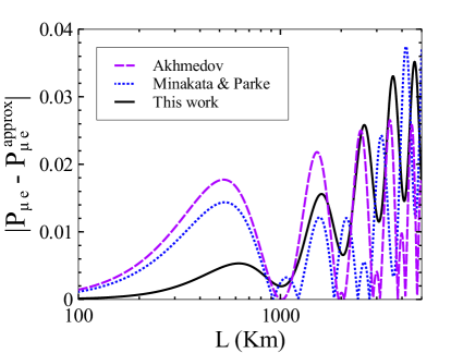
Figure 1: Comparison between the exact neutrino oscillation probability in matter and some approximations. The absolute difference for the electron neutrino survival probability $P_{ee}$ (left panel) and the the muon to electron probability $P_{\mu e}$ (right panel) are plotted against the distance $L$ at an energy of $E_{\nu}=1$ GeV. The central values of the mixing matrix parameters and the square mass differences are taken from [2] and an electron density of $N_{e}=5.92\times 10^{9}$ eV³ has been assumed. The dashed magenta curve accounts for the approximation by Akhmedov [14] as well as the dotted blue curve stands for the expression from Minakata & Parke [15]. The solid curve represents the difference with our approximation at first order.

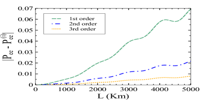
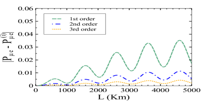
Figure 2: Comparison between the exact formula and our approximation for the neutrino oscillation probability. The absolute differences for $P_{ee}$ (left panel) and $P_{\mu e}$ (right panel) are plotted against the distance $L$, at an energy of $E_{\nu}=1$ GeV. The dashed, dash-dotted and dotted line correspond to the first, second and third order approximation, respectively.

4 Conclusions

In this work, we studied the scenario of the oscillation of three neutrino families propagating through a constant potential caused by matter. First we reconsidered the exact expressions for the oscillation probability, but without any parametrization. Additionally, we found an approximation for these expressions, using the fact that $\Delta m^{2}_{21}\ll\Delta m^{2}_{31}$ and keeping thus the parametrization-free scheme. We found that this result could be expanded to any order in a series expansion, making simple the choice of required precision. Our result is competitive with the ones found in the literature, and its value goes closer to the exact case for short baselines.

References

References

• [1] Y. Fukuda et al. [Super-Kamiokande Collaboration], Phys. Rev. Lett.  81, 1562 (1998) doi:10.1103/PhysRevLett.81.1562 [hep-ex/9807003].
• [2] D. V. Forero, M. Tortola and J. W. F. Valle, Phys. Rev. D 90, 093006 (2014) [arXiv:1405.7540 [hep-ph]].
• [3] J. Schechter and J. W. F. Valle, Phys. Rev. D 22, 2227 (1980).
• [4] W. Rodejohann and J. W. F. Valle, Phys. Rev. D 84, 073011 (2011) [arXiv:1108.3484 [hep-ph]].
• [5] F. J. Escrihuela, D. V. Forero, O. G. Miranda, M. Tortola and J. W. F. Valle, Phys. Rev. D 92, 053009 (2015) doi:10.1103/PhysRevD.92.053009 arXiv:1503.08879 [hep-ph].
• [6] A. de Gouvêa and A. Kobach, arXiv:1511.00683 [hep-ph].
• [7] K. A. Olive et al. [Particle Data Group Collaboration], Chin. Phys. C 38, 090001 (2014).
• [8] S. Parke and M. Ross-Lonergan, arXiv:1508.05095 [hep-ph].
• [9] L. Wolfenstein, Phys. Rev. D 17, 2369 (1978). S. P. Mikheev and A. Y. .Smirnov, Nuovo Cimento Soc. Ital. Fis. C 9, 17 (1986).
• [10] V. D. Barger, K. Whisnant, S. Pakvasa and R. J. N. Phillips, Phys. Rev. D 22, 2718 (1980).
• [11] H. W. Zaglauer and K. H. Schwarzer, Z. Phys. C 40, 273 (1988).
• [12] A. Cervera, A. Donini, M. B. Gavela, J. J. Gomez Cadenas, P. Hernandez, O. Mena and S. Rigolin, Nucl. Phys. B579, 17 (2000) [Nucl. Phys.  B593, 731 (2001)] doi:10.1016/S0550-3213(00)00221-2 [hep-ph/0002108].
• [13] M. Freund, Phys. Rev. D 64, 053003 (2001) [hep-ph/0103300].
• [14] E. K. Akhmedov, R. Johansson, M. Lindner, T. Ohlsson and T. Schwetz, J. High Energy Phys. 04 (2004) 078. [hep-ph/0402175].
• [15] H. Minakata and S. J. Parke, arXiv:1505.01826 [hep-ph].
• [16] K. Asano and H. Minakata, J. High Energy Phys. 06 (2011) 022 doi:10.1007/JHEP06(2011)022 [arXiv:1103.4387 [hep-ph]].
• [17] L. J. Flores and O. G. Miranda, Phys. Rev. D 93, no. 3, 033009 (2016) doi:10.1103/PhysRevD.93.033009 [arXiv:1511.03343 [hep-ph]].