HIFLUGCS: X-ray luminosity – dynamical mass relation and its implications for mass calibrations with the SPIDERS and 4MOST surveys

We present the X-ray luminosity versus dynamical mass relation for 63 nearby clusters of galaxies in a flux-limited sample, the HIFLUGCS (consisting of 64 clusters). The luminosity measurements are obtained based on $\sim 1.3$ Ms of clean XMM-Newton data and ROSAT pointed observations. The masses are estimated using optical spectroscopic redshifts of 13647 cluster galaxies in total. We classify clusters into disturbed and undisturbed ones, based on a combination of the X-ray luminosity concentration and the offset between the brightest cluster galaxy and X-ray flux-weighted center. Given sufficient numbers (i.e. $\geq$45) of member galaxies in computing the dynamical masses, the luminosity versus mass relations agree between the disturbed and undisturbed clusters. The cool-core clusters still dominate the scatter in the luminosity versus mass relation even when a core corrected X-ray luminosity is used, which indicates that the scatter of this scaling relation mainly reflects the structure formation history of the clusters. As shown by the clusters with a small number of spectroscopically confirmed members, the dynamical masses can be underestimated and thus lead to a biased scaling relation. To investigate the potential of spectroscopic surveys to follow up high-redshift galaxy clusters/groups observed in X-ray surveys for the identifications and mass calibrations, we carried out Monte-Carlo re-sampling of the cluster galaxy redshifts and calibrated the uncertainties of the redshift and dynamical mass estimates when only reduced numbers of galaxy redshifts per cluster are available. The re-sampling considers the SPIDERS and 4MOST configurations, designed for the follow-up of the eROSITA clusters, and was carried out for each cluster in the sample at the actual cluster redshift as well as at the assigned input cluster redshifts of 0.2, 0.4, 0.6, and 0.8. For following up very distant cluster/groups, we also carried out the mass calibration based on the re-sampling with only ten redshifts per cluster, and redshift calibration based on the re-sampling with only five and ten redshifts per cluster, respectively. Our results demonstrate the power of combining upcoming X-ray and optical spectroscopic surveys for mass calibration of clusters. The scatter in the dynamical mass estimates for the clusters with at least ten members is within 50%. osmology: observations – Methods: data analysis – Galaxies: kinematics and dynamics – Galaxies: clusters: intracluster medium – Surveys – X-rays: galaxies: clusters

1 Introduction

Galaxy clusters represent the place where astrophysics and cosmology meet: while their overall internal dynamics is dominated by gravity, the astrophysical processes taking place on galactic scales leave observable imprints on the diffuse hot gas trapped within their potential wells (Giacconi et al. 2009). Galaxy clusters (e.g. Vikhlinin et al. 2009a, 2009b; Mantz et al. 2010), in combination with supernovae (e.g. Riess et al. 2011), cosmic microwave background (e.g. Bennett et al. 2013; Hinshaw et al. 2013; Planck Collaboration et al. 2015a), baryon acoustic oscillations (e.g. Dawson et al. 2013) and cosmological weak lensing (e.g. Schrabback et al. 2010; Laureijs et al. 2011; Marian et al. 2011; Heymans et al. 2013), can constrain the dark energy equation-of-state parameter, $w$, at both late and early cosmological epochs. Upcoming experiments such as eROSITA will improve the statistical power of cluster cosmology by a few orders of magnitude (e.g. Predehl et al. 2010; Merloni et al. 2012). However, there are two major challenges in upcoming surveys for high-precision cluster cosmology: accurate mass calibrations and efficient follow-up, such as optical identifications and redshift measurements.

The cluster cosmological applications are degenerate with the mass calibrations of galaxy clusters (e.g. Zhang & Wu 2003; Stanek et al. 2010; Merloni et al. 2012). Large X-ray surveys select galaxy clusters by their observables (e.g. Ebeling et al. 2000; Böhringer et al. 2004; Clerc et al. 2012; Hilton et al. 2012; Takey et al. 2013), particularly the X-ray luminosity ($L$), rather than by their masses ($M$). The $L-M$ relation is required to recover the selection function in terms of cluster masses and predict the cluster masses, hence the cluster mass function. The bolometric X-ray luminosity versus mass relations calibrated with different samples differ significantly (e.g. Chen et al. 2007; Maughan 2007; Pacaud et al. 2007; Pratt et al. 2009; Mantz et al. 2010; Reichert et al. 2011), in which the slope varies from $\sim$1.5 to $\sim$2.0. The predicted numbers of detected clusters in the eROSITA survey based on different calibrations of the $L-M$ scaling relations differ by up to a factor of two (e.g. Pillepich et al. 2012). Apart from the luminosity segregation between cool-core (CC) and non-cool-core (NCC) clusters, merging affects the properties of both the intracluster medium (ICM) and cluster galaxies (e.g. Poole et al. 2006; Evrard et al. 2008), but on different time scales (e.g. Roettiger et al. 1997). Mass estimates from e.g. optical spectroscopy and gravitational lensing, independent of the X-ray luminosity measurement, provide an X-ray blind reference of the cluster mass to calibrate the $L-M$ relation (e.g. Kellogg et al. 1990; Wu et al. 1998, 1999; Zhang et al. 2008; Leauthaud et al. 2010; Israel et al. 2014, 2015; von der Linden et al. 2014). However, the dynamical mass estimates are sensitive to the cluster galaxy selection and member statistic, and overestimate the mass of a merging cluster when the merger axis is along the line of sight (e.g. Biviano et al. 2006; Gifford & Miller 2013; Old et al. 2013; Saro et al. 2013; Wu & Huterer 2013; Rabitz et al. submitted).

The HIghest X-ray FLUx Galaxy Cluster Sample (HIFLUGCS, Reiprich & Böhringer 2002) is a flux-limited sample of 64 clusters selected from the ROSAT All-Sky Survey (RASS; Ebeling et al. 2000; Böhringer et al. 2004). We analyze high-quality XMM-Newton and ROSAT pointed observations as well as optical spectroscopic redshifts of 13650 cluster galaxies for all 64 HIFLUGCS clusters. Excluding 2A 0335+096 with only three redshifts, we present the X-ray luminosity versus dynamical mass relation for the 63 HIFLUGCS clusters, and quantify the impact of mergers as well as CC systems on the $L-M$ relation. A simultaneous mass calibration and cosmological application procedure (e.g. Bocquet et al. 2015; Mantz et al. 2015) can break the degeneracy between them. Such an approach is promising for the use of the combined X-ray and optical surveys in the near future because a vast number of telescopes are dedicated to carry out the optical spectroscopic surveys of galaxy clusters, e.g. eBOSS/SPIDERS (Clerc et al. 2016) and 4MOST. This method, however, relies not only on independent measurements of at least two cluster quantities, e.g. X-ray luminosity and dynamical mass, but also on well understood knowledge on the uncertainties and potential biases in both measured quantities (e.g. Applegate et al. 2014; von der Linden et al. 2014; Planck collaboration 2015b).

Furthermore, efficient follow-up identifications of a large number of galaxy clusters become one of the main tasks in upcoming surveys for high-precision cluster cosmology (e.g. Merloni et al. 2012; Nandra et al. 2013; Pointecouteau et al. 2013). For optimizing the optical spectroscopy follow-up, it is invaluable to investigate in which redshift range existing and upcoming multi-wavelength surveys are suitable to identify groups and clusters of galaxies and to measure their redshifts. For further applications of the optical spectroscopic follow-up, it is worth testing in which redshift range those multi-wavelength surveys can provide accurate dynamical masses that are sufficient for the $L-M$ calibration.

In this paper, we simulate the optical spectroscopic follow-up of clusters by Monte-Carlo (MC) re-sampling of the HIFLUGCS cluster galaxy redshifts in hand according to eight optical spectroscopic setups. We calibrate the redshift and dynamical mass estimates, and quantify in which redshift range the tested optical spectroscopic setups are reliable for measuring the cluster redshifts and dynamical masses. We organize the paper as follows. In Sect. 2 we briefly describe the sample, data and analysis method. The results on the $L-M$ relation of the HIFLUGCS sample are presented in Sect. 3. The results on the redshift and dynamical mass calibrations using simulations of the re-sampled cluster galaxy redshifts are presented in Sect. 4. We summarize our conclusions in Sect. 5. Throughout the paper, we assume $\Omega_{\rm m}=0.3$, $\Omega_{\Lambda}=0.7$, $\sigma_{8}=0.81$, and $H_{0}=70$ km s^-1 Mpc^-1. We quote 68% confidence level. Unless explicitly stated otherwise, we apply the BCES bisector regression method (Akritas & Bershady 1996) taking into account measurement errors on both variables to determine the parameters and their errors in the fit.

2 Sample, data and analysis method

The HIFLUGCS is a sample of galaxy clusters with an X-ray flux limit (0.1–2.4 keV) of $2\times 10^{-11}$  erg/s/cm² and Galactic latitude $|b|>20.0$ degrees covering two thirds of the sky (Reiprich & Böhringer 2002; Hudson et al. 2010), selected from the ROSAT All-Sky Survey (RASS; Ebeling et al. 2000; Böhringer et al. 2004).

2.1 X-ray data and analysis

We analyze nearly $4$ Ms raw data from XMM-Newton for 63 clusters (Zhang et al. 2009, 2011, 2012). After cleaning and selecting the longest observation closest to the cluster center, we obtain $\sim 1.3$ Ms of XMM-Newton data for 59 clusters. We measure the X-ray properties for all 64 clusters in the HIFLUGCS combining XMM-Newton and ROSAT data. The X-ray flux-weighted centroids are listed in Zhang et al. (2011, 2012) with the method described in Sect. 2.3 of Zhang et al. (2010).

2.1.1 X-ray luminosity

The X-ray luminosity is measured within the cluster radius, $r_{500}$, derived from the dynamical mass in Sect. 2.2.2 centered on the X-ray flux-weighted centroid except for 2A 0335+096, which has three galaxy redshifts in total and of which the cluster radius $r_{500}$ is derived from the mass versus gas mass scaling relation. We note that in Zhang et al. (2011) the X-ray luminosity was measured within the $r_{500}$ derived from the gas mass using the total mass versus gas mass scaling relation in Pratt et al. (2009). To suppress the scatter of the $L-M$ relation caused by cool cores, we use the core-corrected X-ray luminosity ($L^{\rm cor}$ hereafter), which is derived from the integration of the surface brightness assuming a constant value of the surface brightness within $0.2r_{500}$ equal to the value at $0.2r_{500}$, $S_{\rm X}(R<0.2r_{500})=S_{\rm X}(0.2r_{500})$, following Zhang et al. (2007). Here $R$ is the projected cluster-centric distance. We note that this correction is only applied in determining the X-ray luminosity. We use the core-corrected bolometric X-ray luminosity (Table 1) for the luminosity versus mass relation of the HIFLUGCS throughout the paper.

Some past work used a radius larger than $r_{500}$ (e.g. Reiprich & Böhringer 2002) to derive the X-ray luminosity, and some used different methods to account for the cool cores (e.g. Pratt et al. 2009). Different methods in deriving the X-ray luminosity may lead to different normalization values of the $L-M$ relation, and also to different slopes. We therefore tabulate the ratios of the X-ray luminosity derived within different annuli for the whole HIFLUGCS of 64 clusters in Table 2. Those values help to ensure a fair comparison between our results and those in other papers. Since the X-ray luminosity varies very little with the truncation radius, the correlation introduced by using the dynamical mass-determined $r_{500}$ in deriving the X-ray luminosity to the $L^{\rm cor}-M$ relation is negligible.

2.2 Optical data and analysis

The positions of the brightest cluster galaxies (BCGs) for 63 clusters are listed in Table 1 in Zhang et al. (2011) and for RXC J1504.1$-$0248 in Zhang et al. (2012). We obtain the velocity of the cluster galaxies from the literature (updated until April 2013, including the compilation in Andernach et al. 2005 and Zhang et al. 2011, 2012). Since the individual error estimates are inhomogeneous, we decided not to weight the calculation of the average velocity. When there is more than one velocity per galaxy available, we calculate an average of the measurements, excluding discordant values and those with large errors.

We checked recent redshift surveys, and found significant ($>90$) numbers of new redshifts for Abell clusters: A2029 from Tyler et al. (2013), A2142 from Owers et al. (2011), A2255 from Tyler et al. (2014), and A2256 from Rines et al. (2016). For 2A 0335+96, NED now offers more redshifts from Huchra et al. (2012), resulting in 14 galaxies between 8400 and 13200 km/s, with a velocity dispersion of about 720 km/s. For NGC 1550, we find 42 galaxies with a velocity dispersion of about 700 km/s.

This work focuses on calibrating the uncertainties of the redshift and dynamical mass estimates when only reduced numbers of galaxy redshifts per cluster are used. The impact on our study by adding these new redshifts mentioned above is negligible. We thus decide to stay with our compilation without update. In our upcoming study, we aim to follow up those clusters with low numbers of spectroscopic members to ensure more than about 45 members for all clusters in the sample in order to derive robust mass estimates for all individual clusters, and calibrate the luminosity versus mass relation taking into account the sample selection effect, i.e. the Malmquist bias (Malmquist 1922) that arises from working with a flux-limited sample. Therefore, we will revise the dynamical mass estimates including these above new redshifts therein.

2.2.1 Cluster galaxy selection

In hierarchical structure-formation scenarios, the spherical infall model predicts a trumpet-shaped region in the diagram of line-of-sight velocity versus projected distance, the so-called caustic (e.g. Kaiser 1987). The boundary of the caustic defines galaxies inside as cluster galaxies and those outside as fore- and background galaxies. For each cluster, we plot the line-of-sight velocity of the selected galaxies as a function of their projected distance from the BCG, and locate the caustic which efficiently excludes interlopers (e.g. Diaferio 1999; Katgert et al. 2004; Rines & Diaferio 2006). We consider only the galaxies inside the caustic as cluster galaxies, and exclude the others from the subsequent analysis. We list the number of cluster galaxies ($n_{\rm gal}$) for the HIFLUGCS in Table 1. We gathered redshifts of a total of 13650 cluster galaxies after the caustic member selection. Since 2A 0355+096 has only three redshifts, we excluded it from the study involving cluster redshift and dynamical mass estimates. The median number of spectroscopic members for the remaining sample is 188 per cluster.

There are another six clusters that have fewer than 45 cluster galaxies with spectroscopic redshifts in the HIFLUGCS (i.e. 13 galaxies for A0478, 22 for NGC1550, 42 for EXO 0422$-$086, 37 for Hydra A, 20 for S1101, and 44 for A2597), which were maintained in the redshift and dynamical mass study. All six systems with $<45$ cluster galaxy redshifts are CC clusters. The reason for having $<45$ cluster galaxy redshifts is that these clusters are not covered by large spectroscopic surveys such as SDSS or 2dF/6dF. We aim to observe them with ground-based telescopes. Recently, we obtained new redshifts from VLT/VIMOS for Abell S1101 (Rabitz et al. submitted).

2.2.2 Redshift, dynamical mass and cluster radius

We apply the bi-weight estimator (e.g. Beers et al. 1990) to the cluster galaxies to measure the cluster redshift ($z$) and velocity dispersion ($\sigma$). The errors are estimated through 1000 bootstrap simulations.

The caustic method mentioned in Sect. 2.2.1 can provide an estimate of the escape velocity and thus the matter distribution for the halo according to the distribution of the caustic amplitude (e.g. Diaferio 1999). However, only with a large number of spectroscopic members, e.g. $\sim$200 members, one is likely to recover a rather complete sampling of the caustic, which yields a robust measurement of the underlying dark matter distribution of the cluster as shown by the simulations in e.g. Serra & Diaferio (2013). Their simulations also show that a lower number of members thus tends to provide a slightly reduced amplitude of the caustic due to under-sampling of the caustic, which causes underestimation of the total mass.

To optimize optical spectroscopic follow-up for galaxy clusters, particularly at high redshifts where the cluster galaxy member statistic is low, we focus on the method to derive the dynamical mass based on a small number of cluster galaxies, differing from the caustic method. There are a number of such methods calibrated by samples of simulated clusters (e.g. Biviano et al. 2006; Munari et al. 2013). We note that the difference between the dynamical masses derived with those methods is rather small which is within the uncertainties of our dynamical mass estimates. Apart from this, we focus only on the relative variation in the dynamical mass measurements that is normalized to the input dynamical mass in the investigations of the systematic bias and uncertainties of redshift and dynamical mass estimates based on MC re-sampling (Sect. 4).

Our method of mass estimation is based entirely on the velocity dispersion estimate as explained in Sect. 3 of Biviano et al. (2006, $M_{\sigma}$ therein). We follow the Navarro, Frenk & White (NFW, 1997) model used in Biviano et al. (2006) to derive $M_{500}$ from $M_{\sigma}$. The dimensionless Hubble parameter, $E(z)=\sqrt{\Omega_{\rm m}(1+z)^{3}+\Omega_{\Lambda}}$, is added to their formulation since not all our clusters are at $z\sim 0$. In this work, we use the dynamical mass at the radius within which the over-density is 500 times the critical density as the cluster mass ($M_{500}$, Table 1). We derive the cluster radius ($r_{500}$) from the dynamical mass ($M_{500}$), different from the method used by Zhang et al. (2011).

2.3 Cluster morphology

Although the cluster properties are driven by gravity, predominantly from dark matter, the baryon physics on small scales modifies the scaling relation from the self-similar prediction through cooling, merging and feedback from star formation and AGN activities. We divided the HIFLUGCS into undisturbed versus disturbed subsamples as well as CC and NCC subsamples in order to study the impact of mergers and CC clusters, respectively, on our results.

2.3.1 Undisturbed versus disturbed clusters

Many studies found that a large offset between the BCG and X-ray peak/centroid likely indicates that more merging has happened in the past (e.g. Katayama et al. 2003; Hudson et al. 2010; Zhang et al. 2010, 2011). We convert the angular separation between the X-ray flux-weighted center and BCG position into the physical separation at the cluster redshift for all 64 clusters in the HIFLUGCS. As shown in Zhang et al. (2011), the offset in projection between the X-ray flux-weighted center and BCG position scaled by the cluster radius, ${\Delta}R/r_{500}$, serves rather well to separate the disturbed from the undisturbed clusters.

The luminosity concentration is also one of the parameters suitable to separate the clusters (e.g. Santos et al. 2008). Here we set this parameter to be $c_{\rm L}=L(R\leq r_{500})/L(R\leq 0.2r_{500})$, and we integrate the surface brightness within a projected cluster-centric distance of $r_{500}$ and $0.2r_{500}$ to derive the bolometric X-ray luminosity of $L(R\leq r_{500})$ and $L(R\leq 0.2r_{500})$, respectively. All HIFLUGCS clusters have also Chandra data, but mainly in the field of the cluster cores, not even out to $0.2r_{500}$ for a number of cases. We thus prefer to rely on XMM-Newton data to compute the $c_{\rm L}$ parameter.

In the following we combine the cuts of $c_{\rm L}$ and ${\Delta}R/r_{500}$ to effectively separate the sample into undisturbed and disturbed clusters. As shown in Fig. 1 and Table 3, the histograms of both $\log_{10}c_{\rm L}$ and $\log_{10}({\Delta}R/r_{500})$ of the 64 clusters follow approximately Gaussian distributions. The best power-law fit between the two parameters for the 64 clusters is $\log_{10}c_{\rm L}=(0.593\pm 0.053)+(0.125\pm 0.028)\log_{10}({\Delta}R/r_{500})$. We divide the whole sample into disturbed and undisturbed clusters using the 1$\sigma$-clipping of the Gaussian-mean values of these two histograms. Those with low values of both $c_{\rm L}$ and ${\Delta}R/r_{500}$ are considered as undisturbed clusters (see the right panel of Fig. 1). The cuts divide the sample into 39 undisturbed clusters and 24 disturbed clusters.

2.3.2 CC versus NCC clusters

The gas mass versus total mass relation in recent work (e.g. Arnaud et al. 2005; Zhang et al. 2008) shows a slope shallower than unity, the self-similar prediction, which may be accounted for by the mass dependence of the gas mass fraction in CC and NCC systems (e.g. Eckert et al. 2012). Therefore, we also investigate our results for the subsamples of CC and NCC clusters, respectively.

The central cooling time can be accurately estimated from Chandra data because of its smaller point-spread function (PSF). We used the central cooling time calculated at $0.004r_{500}$ from Eq. (15) in Hudson et al. (2010), and divided the sample of the 64 clusters into 28 CC clusters and 36 NCC clusters as listed in Table 2 in Zhang et al. (2011).

3 X-ray luminosity versus dynamical mass

We carried out the X-ray and optical analyses independently, apart from taking the dynamical mass-determined $r_{500}$ in computing the X-ray bolometric luminosity. Since the luminosity values measured within $r_{500}$ and 2.5$r_{500}$ differ only by $\sim$15% on average as shown in Table 2, using the cluster radius, $r_{500}$, derived from the dynamical mass, in computing the X-ray bolometric luminosity shall not cause any significant bias in our result.

We fit the $L^{\rm cor}-M$ relation by a power-law,

$$\log_{10}\widetilde{L}=A\log_{10}\widetilde{M}+B\leavevmode\nobreak\ ,$$ (1)

in which $\widetilde{L}=\frac{L^{\rm cor}}{E(z)10^{44}{\rm erg/s}}$ and $\widetilde{M}=\frac{M\,E(z)}{10^{14}M_{\odot}}$. Note that the HIFLUGCS is a flux-limited sample, which consists of clusters covering a broad range of redshifts (i.e. from $z=0.0037$ to $z=0.2153$). Therefore, we include the $E(z)$ factor in the scaling relation to account for the evolution of the geometry of the Universe in this redshift range. We assume a constant standard deviation of the luminosity from this relation in logarithmic scale, and use $\sigma_{\log_{10}L}$ for the intrinsic scatter of the luminosity in logarithmic scale. We choose the relatively simple algorithm given in Akritas & Bershady (1996) to perform the fit to the relation $y=Ax+B$, in which

$$\chi^{2}=\sum_{i}\frac{(y_{i}-Ax_{i}-B)^{2}}{\sigma^{2}_{y,i}+A^{2}\sigma^{2}_{x,i}}\leavevmode\nobreak\ .$$ (2)

The scatter of $y$ consists of two components, the statistical and intrinsic scatter, which satisfy $\sigma^{2}_{y,i}=\sigma^{2}_{y,i,{\rm sta}}+\sigma^{2}_{y,i,{\rm int}}$ (e.g. Weiner et al. 2006). In Table 4, we list the best-fit parameters also including the normalization values setting the slope to the self-similar prediction, namely 4/3. Note that the data are still in agreement with a slope of 4/3 within $2\sigma$ uncertainties of the best-fit slope parameters.

3.1 $L^{\rm cor}-M$ relation for the $n_{\rm gal}\geq 45$ clusters

The dynamical masses tend to be underestimated for the clusters with too few redshift measurements according to the clusters in simulations (e.g. Biviano et al. 2006; Zhang et al. 2011). The effect becomes negligible (i.e. on a level of a few per cent) when clusters with a sufficient number of spectroscopic cluster galaxies are considered.

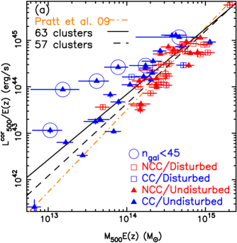
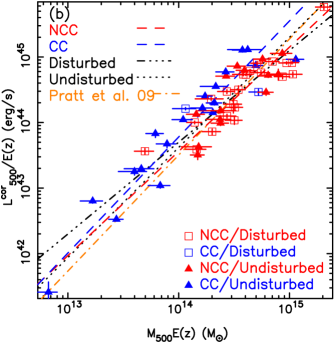
Figure 2: (a) Core-corrected bolometric X-ray luminosity versus dynamical mass for the 63 clusters with the best power-law fits for the 63 and 57 ($n_{\rm gal}\geq 45$) clusters as black solid and dashed lines, respectively. (b) Core-corrected X-ray bolometric luminosity versus dynamical mass for the 57 ($n_{\rm gal}\geq 45$) clusters with the best power-law fits for the NCC, CC, disturbed, and undisturbed clusters as red dashed, blue dashed, black dot-dot-dot-dashed, and black dotted lines, respectively.

In Zhang et al. (2011) we found that the velocity dispersion measurements, and thus the dynamical masses, may be significantly underestimated for the clusters with fewer than 45 spectroscopic member galaxies in the sample. To avoid any bias due to extreme outliers with too few cluster galaxies with spectroscopic redshifts, we show the $L^{\rm cor}-M$ relations for the 63 clusters (Fig. 2a) and for the 57 clusters that have at least 45 cluster galaxies with spectroscopic redshifts (Fig. 2b), respectively. For the 63 clusters, the slope, $1.29\pm 0.09$, agrees with the self-similar prediction. However, most recent work shows steeper slopes, e.g. $1.77\pm 0.07$ in Pratt et al. (2009). Taking a close look, the systems with very few redshifts appear to cause the shallow slope. In contrast to that of the 63 clusters, the slope of the 57 clusters is steeper. The selection effect, i.e. the Malmquist bias that should be corrected for a flux-limited sample, should lead to an even steeper slope for the 57 clusters, which tends to be in better agreement with recent X-ray calibrated $L-M$ relations (e.g. Pratt et al. 2009). At the same time, the fact that the six discarded clusters are all CC clusters may also have an impact on the total best-fit slope, although there appears little difference between the slopes of the $L-M$ relations between CC and NCC clusters.

3.2 $L^{\rm cor}-M$ relations for the CC/NCC and undisturbed/disturbed subsamples

We list the best-fit $L^{\rm cor}-M$ relations regarding cluster classification in Table 4. As shown in Fig. 2b and Fig. 3, the NCC clusters are under-sampled in the low-mass regime since the HIFLUGCS is a flux-limited sample. The slope parameters agree within 1$\sigma$ error between the undisturbed and disturbed clusters as well as between the CC and NCC clusters. Note that there is no obvious mass dependence in the scatter of the core-to-total luminosity ratio (actually $1/c_{\rm L}$) for the CC and NCC subsamples, respectively, as shown in Fig. 3. The $L^{\rm cor}-M$ relation for the disturbed clusters has smaller intrinsic scatter than that for the undisturbed clusters. Also the intrinsic scatter of the NCC clusters is smaller than that of the CC clusters even when the core-corrected luminosity is in use. Note that this partially depends on how broad the used cut is to classify the corresponding cluster subsamples. The normalization of the disturbed (NCC) clusters is in better agreement with the X-ray calibrated relation (e.g. Zhang et al. 2008, see Table 3 therein; Pratt et al. 2009). Assuming a fixed slope of 4/3, the normalization agrees between different cluster types within the uncertainties.

A comparison of the best fits for the undisturbed (CC) clusters in the samples of the 57 and 63 clusters in Fig. 2 shows clearly that the scatter for the undisturbed (CC) clusters in the sample of 57 clusters with $N_{\rm gal}>45$ is lower than that for the sample of 63 clusters. As shown in Fig. 2b for the 57 clusters, the normalization on average agrees within 17% between the undisturbed and disturbed clusters, and within 32% between the CC and NCC clusters. The slopes still agree among the subsamples. As the scatter is dominated by the CC clusters, the scatter of the $L^{\rm cor}-M$ relation may mainly be due to the integrated effect of the structure formation history instead of recent extreme merging.

4 Systematic bias and uncertainties of redshift and dynamical mass estimates based on MC re-sampling

The results from our sample show that the clusters with low numbers of spectroscopic members tend to have their dynamical masses underestimated. It is thus of prime importance to quantify any systematic bias and uncertainties of the dynamical mass estimate and their implications on mass calibrations using upcoming optical spectroscopic surveys.

Both large optical spectroscopic surveys and individual pointed observations will be used to follow up galaxy clusters detected in upcoming large X-ray surveys, e.g. eROSITA. The huge amount of optical spectroscopic follow-up data could be potentially combined with the X-ray data for mass calibrations, in particular, in different redshift ranges. This allows to constrain the evolution of the mass scaling relations, which becomes important when using high-redshift clusters for cosmology. In the following, we calculated the cluster redshift and estimated the dynamical mass using subsamples of member galaxies which we re-sampled according to eight optical spectroscopic setups, which demonstrates their ability for studying mass calibrations using the follow-up of the X-ray detected clusters. We note that the re-sampled galaxies are selected from the catalog of the caustic-bounded galaxies. Therefore, the probability of contamination from interlopers is low. The systematic uncertainties are mainly caused by statistical fluctuations in the re-sampling. Our study is also useful to assign the mass uncertainty in the stacking analysis using cluster samples with a rather clean member selection but a small number of members (e.g. Clerc et al. submitted).

4.1 Optical spectroscopic survey setups

The Extended Baryon Oscillation Spectroscopic Survey (eBOSS; e.g. Schlegel et al. 2011) is a redshift survey covering a wavelength range from 340 nm to 1060 nm, with a resolution $R=3000-4800$. This survey targets objects up to redshift 2. With the eBOSS setup, the SPectroscopic IDentification of ERosita Sources (SPIDERS; e.g. Merloni et al. 2012) survey has been designed to follow up X-ray selected active galactic nuclei (AGN) and clusters over $\sim$7500 degree² area. Before eROSITA data will be available, SPIDERS is targeting ROSAT and XMM-Newton sources (see Clerc et al. submitted; Dwelly et al. in prep.). In the later years of operations, SPIDERS will target eROSITA sources detected in the first two years of observations (see Merloni et al. 2012). The 4-metre Multi-Object Spectroscopic Telescope (4MOST, e.g. de Jong et al. 2012) is designed to obtain $>$1 million redshifts for $>$50,000 clusters in the Southern sky in the eROSITA survey. The Euclid mission can follow up high-redshift galaxies through their emission lines (e.g. Laureijs et al. 2011; Pointecouteau et al. 2013). In this study, however, we will not discuss the optimization of the follow-up of the Euclid survey since Euclid provides slitless spectroscopy, which has no fiber constraint. Euclid will rather focus on, for example, how to improve the situation due to overlapping spectra in densely populated regions for optimizing its strategy.

In practice, only a number of cluster galaxies per cluster can be targeted given a fiber spacing constraint for multi-object spectroscopic surveys. Moreover, toward the high-redshift regime, a bright limiting magnitude cut can strongly limit the number of spectroscopic members. To disentangle the two effects, we perform the investigations in two steps: (i) for the setups using the closest fiber separation alone and (ii) for the setups including constraints from both the closest fiber separation and limiting magnitude cuts. SPIDERS uses actually a minimum fiber separation of 65^′′. To demonstrate the impact of the fiber separation, we use a fiber spacing constraint of 55^′′ and 65^′′, respectively, in our MC simulations for SPIDERS. Note that the limiting magnitude is actually the fiber magnitude. Toward the very high-redshift regime, optical spectroscopy of several of the bright galaxies already requires high-sensitivity optical spectrographs, e.g. on the Very Large Telescope (VLT). We also investigate the setups with a limited number of cluster redshifts. Below are the eight setups, in which the BCG is always first selected for targeting.

1. SPIDERS_55: It has a closest fiber separation of 55^′′. Each position can be pointed only once.

2. SPIDERS_65: It has a closest fiber separation of 65^′′. Each position can be pointed only once.

3. 4MOST: It has a closest fiber separation of 20^′′. Each position can be pointed four times.

4. SPIDERS_55m: It has a closest fiber separation of 55^′′. Each position can be pointed only once. The limiting magnitude is $i_{\rm AB}=21$.

5. SPIDERS_65m: It has a closest fiber separation of 65^′′. Each position can be pointed only once. The limiting magnitude is $i_{\rm AB}=21$.

6. 4MOSTm: It has a closest fiber separation of 20^′′. Each position can be pointed four times. The limiting magnitude is $r_{\rm AB}=22$.

7. 10zs: It samples the BCG and nine randomly selected remaining member galaxies per cluster.

8. 05zs: It samples the BCG and four randomly selected remaining member galaxies per cluster.

4.2 Input cluster redshifts, $z_{\rm in}$, in the I–VI setups

Follow-up of high-redshift systems is particularly important to constrain the evolution of mass calibrations that is still poorly understood. Technically, nearby clusters can tolerate large values of the closest fiber separation in the optical spectroscopy. The angular size of a cluster decreases toward high redshift. The number of spectroscopic members decreases with redshift given a fixed value of the closest fiber separation. Therefore, we tested the I–VI setups assuming input cluster redshifts at the HIFLUGCS cluster redshifts ($z$ in Table 1) as well as placing the clusters at the redshift values of 0.2, 0.4, 0.6, and 0.8, respectively. We note that the relative rest-frame line-of-sight velocity of any member galaxy to its host cluster is not modified in this process.

4.3 Limiting magnitude cuts in the IV–VI setups

We included the limiting magnitude cuts in re-sampling the member galaxies in the IV–VI setups as follows.

4.3.1 Shape of the galaxy luminosity function (GLF)

We assume that the observed spectroscopy member galaxies are those at the bright end of the GLF. We adopted the Schechter function fit of the GLF of the bright galaxies within a projected cluster-centric distance of 2 Mpc in the $i$- and $r$-bands (Popesso et al. 2005, Table 2, local background) for the SPIDERS and 4MOST surveys, respectively. Given the results in Hansen et al. (2009), we assume that the shape of the GLF of the bright red members does not change with cluster-centric radius for simplicity.

4.3.2 Normalization of the GLF

There are a number of richness versus mass calibrations (e.g. Hansen et al. 2005, 2009; Johnston et al. 2007; Reyes et al. 2008). We take the richness versus weak-lensing mass calibration given by Eq. (10) in Hansen et al. (2009), in which the masses are measured within the radius where the mass over-density is 200 relative to the critical density, and calculate the richness from the cluster dynamical mass for each HIFLUGCS cluster.

For simplicity, we assume that the red member galaxies brighter than $(i^{\ast}+1)$ are similar to those brighter than $(r^{\ast}+1)$. Therefore, the number of the red member galaxies brighter than $(i^{\ast}+1)$ is similar to the number of the red members brighter than $(r^{\ast}+1)$. We obtain the richness by integrating the GLF down to $(i^{\ast}+1)$ magnitude for the SPIDERS survey and $(r^{\ast}+1)$ magnitude for the 4MOST survey, respectively. Assuming the richness obtained from the dynamical mass equal to the richness derived by integrating the GLF, we obtain the normalization of the GLF.

4.3.3 Galactic extinction and $K$-corrections

We correct apparent magnitudes for Galactic extinction using the maps of Schlegel et al. (1998). We assume that photometric errors at bright magnitudes are 0.05. We use typical colors and their color uncertainties of luminous red galaxies of Maraston et al. (2009), and apply $K$-correction and evolutionary correction using the luminous red galaxy template in kcorrect (v4_2, Blanton & Roweis 2007).

4.3.4 Member selection

The maximum number of member galaxies, $n_{\rm max}$, that can be spectroscopically followed-up is computed by integrating the GLF down to the limiting magnitude. In Sect. 4.3.1, we simply assumed that the observed spectroscopy member galaxies are those filling in the bright end of the GLF. Therefore, if the number of cluster members for the HIFLUGCS clusters ($n_{\rm gal}$ in Table 1) is larger than $n_{\rm max}$, the fraction of the $n_{\rm gal}$ spectroscopic members that are brighter than the limiting magnitude is $f_{\rm obs}=n_{\rm max}/n_{\rm gal}$; otherwise, all existing spectroscopic members are brighter than the limiting magnitude, $n_{\rm max}=n_{\rm gal}$.

Note that many cluster members in the observational sample have no $i$- and $r$-magnitudes from the NED. As a preliminary selection, we first take the BCG, and then randomly take $f_{\rm obs}n_{\rm gal}-1$ additional spectroscopic members using the MC method. The initially selected members are filtered further according to the values of the closest fiber separation.

4.3.5 Impact of flux loss of the aperture magnitude

The angular sizes of very bright cluster galaxies in the nearby Universe (i.e. $z<0.4$) are usually larger than the fiber aperture. The flux-loss correction may become important in deriving the apparent magnitudes from the measured flux in the fiber aperture when considering the limiting magnitude cut. Additionally, the PSF affects the measured apparent magnitudes due to convolution of galaxy images caused by the seeing. As shown by our model of the flux loss in targeting galaxies with spectroscopic fibers in Appendix A, this effect is negligible and skipped in our further analyses.

4.4 Redshift and dynamical mass measurements

To estimate the average of the systematic uncertainties, we carried out 500 re-sampling runs per cluster per setup per input cluster redshift ($z_{\rm in}=z,0.2,0.4,0.6,0.8$ for I–VI setups and $z_{\rm in}=z$ for VII–VIII setups). In each run, we measured the cluster redshift, velocity dispersion and dynamical mass following the procedure in Sect. 2.2.2 when the number of re-sampled members reach ten, $n_{{\rm gal},i}\geq 10$. Otherwise ($n_{{\rm gal},i}<10$), we only compute the cluster redshift, which is the mean of the member galaxy redshifts, but not the velocity dispersion and dynamical mass.

The Gaussian mean and bi-weight (see Sect. 2.2.2) mean values of the histograms of the redshift and dynamical mass estimates from 500 runs based on the re-sampled members agree well in all cases apart from the 10zs setup. The bi-weight mean of the histograms is in general closer to the input value than the Gaussian mean for the 10zs setup. Therefore, we use the bi-weight mean for calculating the results. The number of member redshifts used per cluster per setup per input cluster redshift, $n_{{\rm gal},MC}$, is computed as the bi-weight mean of $n_{{\rm gal},i}$ with $i=0,...,499$. As one may obtain $n_{{\rm gal},i}<10$ for some re-sampling runs, $n_{{\rm gal},MC}$ can be fewer than ten for some cases involving the dynamical mass estimates, in which the dynamical mass per cluster per setup per input cluster redshift, $M_{\rm 500,MC}$, is computed as the bi-weight mean of $M_{500,j}$ with $j=i$ if $n_{{\rm gal},i}\geq 10$. Simulated clusters with less than ten members are excluded in the mass computation.

4.5 Summary of results

4.5.1 Fraction of selected members

Using the collisional distance constraint alone (setups I–III), almost all members were selected in the 4MOST setup, and more than 95% of the members were selected in the SPIDERS_55 and SPIDERS_65 setups. In the case of ten/five redshifts per cluster, only a small fraction of the members are selected. The fraction of selected members including the limiting magnitude cut (setups IV–VI) decreases faster toward high-redshift end than that in the re-sampling assuming only the collisional distance constraint.

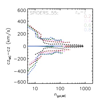
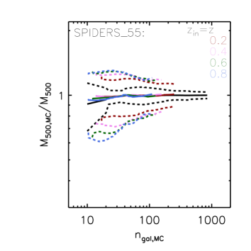
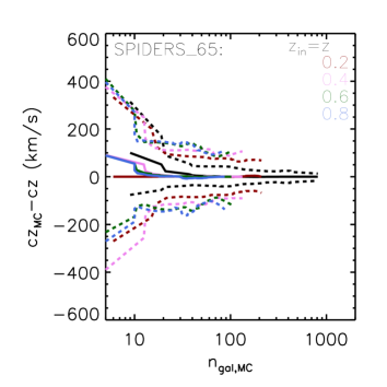
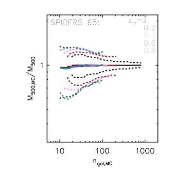
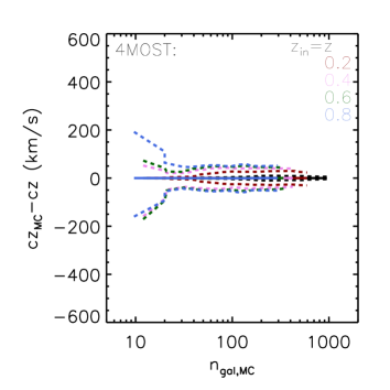
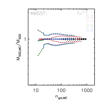
Figure 4: Bias (solid lines) and dispersion (dashed lines) of the redshift (left panels) and dynamical mass (right panels) measurements in the SPIDERS_55 (upper panels), SPIDERS_65 (middle panels) and 4MOST (lower panels) setups from the input cluster values as a function of the re-sampled number of redshifts in use. The curves are smoothed with a boxcar average of the specified width of 11 to avoid spikes due to under-sampling for a few clusters.

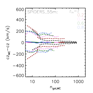
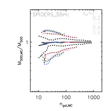
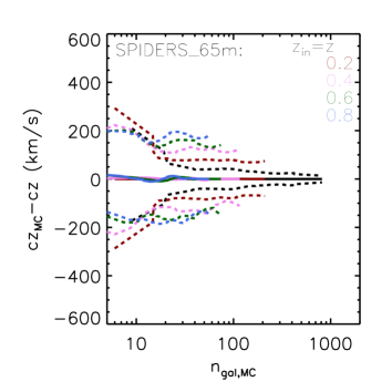
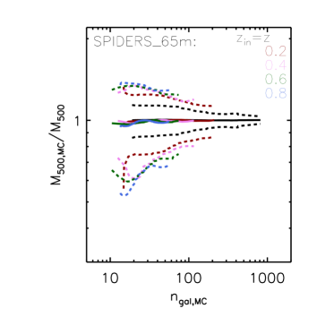
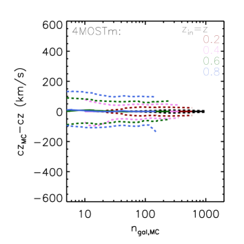
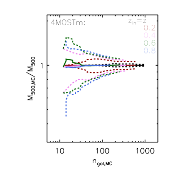
Figure 6: Bias (solid curves) and dispersion (dashed curves) of the redshift (left panels) and dynamical mass (right panels) measurements in the SPIDERS_55m (upper panels), SPIDERS_65m (middle panels) and 4MOSTm (lower panels) setups from the input cluster values as a function of the re-sampled number of redshifts in use. The curves are smoothed with a boxcar average of the specified width of 11 to avoid spikes due to under-sampling for a few clusters.

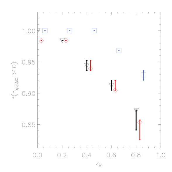
Figure 7: Fraction of the clusters with at least ten redshifts per cluster after the re-sampling using the SPIDERS_55m (black triangles), SPIDERS_65m (red diamonds, with 0.03 offset) and 4MOSTm (blue squares, with 0.06 offset) setups as a function of the assigned input cluster redshift ($z_{\rm in}$) in the re-sampling. Note that $z_{\rm in}=0$ case refers to the re-sampled clusters at the cluster redshifts $z$.

As shown in the right panels of Figs. 4–6 the scatter in the dynamical mass estimates for the clusters with at least ten members is within 50%, which is the minimum required precision for a stacking analysis for the mass calibration given the known intrinsic scatter in the mass–observable relation (e.g. Biviano et al. 2006). We thus inspect the fraction of the clusters with at least ten members. All of the 63 clusters in the SPIDERS and 4MOST cases that assume no magnitude cut have more than ten galaxy members per cluster. In the setups with the magnitude limit instead, the fraction of the clusters with at least ten members per cluster decreases with redshift as shown in Fig. 7. In the redshift bins of 0.2, 0.4, 0.6, and 0.8 in the SPIDERS_55m setup, there are one, three, eight, and 18 clusters out of 63 clusters, which have fewer than ten redshifts per cluster. The case for the SPIDERS_65m setup, which uses a larger fiber separation ($65^{\prime\prime}$), is slightly worse. In the redshift bins of 0.4, 0.6 and 0.8 using the 4MOSTm setup, there are one, two and four clusters out of 63 clusters, which have fewer than ten redshifts per cluster.

4.5.2 Redshift estimates

We considered all clusters with $n_{\rm gal,MC}>1$ in the redshift estimates. Here we do not consider $n_{\rm gal,MC}=1$ clusters because the BCG is always taken according to the selection method (Sect. 4.3.4) which leads to zero dispersion based on 500 MC realizations. The cluster redshifts are well recovered to a level of a few per cent in all cases. There is no obvious systematic dependence on the cluster redshift. The left panels of Figs. 4–6 and Fig. 8 show the bias of the redshifts obtained in the re-sampled procedure from the input cluster redshifts and its dispersion based on the 500 MC realizations. We note that the catalog of the galaxy redshifts of the HIFLUGCS is a rather clean member galaxy input catalog, likely almost free of interlopers. Uncertainties derived from the scatter in the down-sampling thus do not account for the effect of interlopers. This artificially restricts the uncertainties of the redshift estimates to less than 0.01. In Figs. 5 and 8, the scatter increases slightly with the number of the input galaxies, which may indicate that the scatter of redshift with a fixed number of spectroscopic members depends on the richness. Richness-dependent values of minimum numbers of galaxy redshifts for different richness populations may thus be required for a stacking analysis in order to ensure an equivalent scatter introduced by individual systems in the redshift estimates.

4.5.3 Dynamical mass estimates

There is no redshift or mass dependence in the systematic uncertainties of the dynamical mass estimates. The right panels of Figs. 4–6 show the bias of the dynamical mass estimates obtained in the re-sampled procedure from the cluster total mass and its dispersion based on the 500 MC realizations. Here we do not consider $n_{{\rm gal},i}<10$ realizations as noted in Sect. 4.4. Therefore, toward the low-$n_{\rm gal,MC}$ end, the bias and dispersion is slightly underestimated as not all 500 MC realizations can be used.

The dynamical mass is well recovered with less than $\sim$20% bias on average. The dispersion in Figs. 4–6 demonstrates the precision the corresponding setup can reach as a function of redshift. This information can be used for the sample selection corresponding to the required precision for the purpose of mass calibration in upcoming surveys. Given the same required accuracy, the 4MOST survey can provide mass calibration up to a higher redshift compared to the SPIDERS survey. With ten redshifts per cluster, the dynamical mass measurement can easily be biased by a factor of two for individual clusters, which would not be suitable for a robust mass calibration unless stacking them. Similar to that shown in the redshift estimates, the scatter increases again slightly with the number of the input galaxies, this may indicate a dependence on richness. Richness dependent cuts of minimum numbers of galaxy redshifts in different richness bins shall also be required for a stacking analysis to ensure an equivalent scatter introduced by individual systems in the dynamical mass estimates.

4.5.4 Limitations

The current paper describes an ideal situation of using an input member catalog almost free from contamination from interlopers for the spectroscopic follow-up that does not represent the reality in general. According to real surveys, we need to construct our input galaxy candidate sample for the spectroscopic follow-up, which can not avoid contamination from, for example, interlopers. Additionally, we need to select a number of certain member galaxies from a large catalog for the follow-up to determine the redshift and velocity dispersion, which requires knowledge of the selection effects for recovering the mass estimates robustly. The input member galaxy sample for the simulation in the current paper, however, likely contains no interlopers. We also can not quantify the selection effect as the sample is a collection of clusters from the available literature, instead of e.g. a spectroscopic follow-up of a well-defined photometric galaxy member sample. A further study based on mock data in simulations with known selection functions as well as sufficient fore- and background galaxies in the galaxy sample will help to address these questions. Another limitation is that clusters may evolve from $z=0.8$ to the present epoch, an effect that is not fully accounted for by simply shifting the HIFLUGCS clusters to higher redshifts. It is thus not obvious that the HIFLUGCS sample is the best test-case for the forecasts of the 4MOST and SPIDERS surveys at higher redshifts.

5 Conclusions

We analyzed $\sim 1.3$ Ms of clean XMM-Newton data and ROSAT pointed observations as well as optical spectroscopic redshifts of 13650 cluster member galaxies for all 64 HIFLUGCS clusters. Excluding 2A 0335+096 with only three redshifts, we present the $L^{\rm cor}-M$ relation for 63 nearby clusters of galaxies in the HIFLUGCS. For the optimal use of the optical spectroscopic surveys for high-redshift galaxy clusters and groups observed in upcoming X-ray surveys for mass calibrations, we carried out MC re-sampling of the galaxy members with spectroscopic redshifts, and calibrated the systematic uncertainties in the redshift and dynamical mass estimates. We predicted the redshift and dynamical mass estimates assuming the SPIDERS and 4MOST optical spectroscopic survey setups, respectively, using MC re-sampling of the 63 HIFLUGCS clusters by placing the sample at the actual cluster redshifts as well as at the redshifts of 0.2, 0.4, 0.6, and 0.8. Aiming for high-redshift cluster/group systems, we also predicted the redshift estimates based on five and ten spectroscopic members per cluster, respectively, and the mass estimates based on ten spectroscopic members per cluster. We list the conclusions in detail as follows.

• Given sufficient numbers (i.e. $\geq$45) of member galaxies in computing the dynamical masses, the $L^{\rm cor}-M$ relations agree between the disturbed and undisturbed clusters.

• The CC clusters still dominate the scatter in the $L^{\rm cor}-M$ relation even when the CC corrected X-ray luminosity is used. This indicates that the scatter of the $L^{\rm cor}-M$ scaling relation mainly reflects the structure formation history of the clusters.

• The dynamical masses can be measured within 10% uncertainty using the SPIDERS_55, SPIDERS_65 and 4MOST setups which is independent of cluster redshift and mass. With ten redshifts per cluster or more, the dynamical masses can be recovered with less than 20% bias on average, in which the dynamical masses are underestimated for most systems.

• The bias of the cluster dynamical mass estimates increases toward the high-redshift end. The underestimation of the cluster masses on average using the SPIDERS_65m setup, in which both the collisional distance of 65^′′ and magnitude cut are considered, is better than 19%, 28%, 34%, and 37% in the redshift bins of 0.2, 0.4, 0.6, and 0.8. The dynamical mass is recovered with less than 20% underestimation up to redshift 0.6 using the 4MOSTm setup, in which both the collisional distance and magnitude cut are considered. In the redshift bin of 0.8, the underestimation of the dynamical masses on average, according to the 4MOSTm setup, is still less than 24%. Assuming the SPIDERS_55m (4MOSTm) setup, the dynamical masses can be used as an independent reference blind to the X-ray observables to calibrate the cluster mass with less than 20% underestimation up to redshift 0.2 (0.6) with 2% (3%) catastrophic outliers (i.e. fewer than ten members per cluster) in upcoming X-ray surveys. Empirically, one can correct this bias using a complete sample from observations or a mock sample in simulations, which includes the causes of the bias such as contamination from fore- and background galaxies.

Table 1: Number of spectroscopic redshifts, velocity dispersion, dynamical mass, core-corrected X-ray bolometric luminosity, luminosity concentration and offset between the BCG and X-ray flux-weighted centroid for the whole HIFLUGCS sample of 64 clusters sorted by R.A. as shown in Table 1 in Zhang et al. (2011).

Name	$n_{\rm gal}$	$\sigma$ (km/s)	$M_{500}$ ($10^{14}M_{\odot}$)	$L^{\rm cor}_{500}$ ($10^{44}$ erg/s)	$c_{\rm L}$	${\Delta}R/r_{500}$
A0085	350	$963\pm 39$	$4.83\pm 0.76$	$7.60\pm 0.43$	2.089	0.002
A0119	339	$797\pm 38$	$2.67\pm 0.47$	$3.03\pm 0.21$	5.383	0.014
A0133	137	$725\pm 44$	$1.98\pm 0.42$	$1.45\pm 0.09$	1.809	0.027
NGC0507	110	$503\pm 33$	$0.68\pm 0.15$	$0.11\pm 0.01$	2.062	0.014
A0262	138	$527\pm 30$	$0.78\pm 0.16$	$0.48\pm 0.06$	2.705	0.006
A0400	114	$647\pm 40$	$1.44\pm 0.30$	$0.39\pm 0.03$	3.499	0.005
A0399	101	$1223\pm 75$	$10.37\pm 2.18$	$5.63\pm 0.48$	2.415	0.056
A0401	116	$1144\pm 74$	$8.32\pm 1.82$	$11.76\pm 0.91$	2.248	0.015
A3112	111	$740\pm 63$	$2.09\pm 0.57$	$3.68\pm 0.19$	1.569	0.024
NGC1339/Fornax	339	$366\pm 13$	$0.27\pm 0.04$	$0.03\pm 0.00$	2.595	0.001
2A 0335$+$096	3	—	—	$1.43\pm 0.12$	0.130	0.006
III Zw 054	45	$657\pm 62$	$1.49\pm 0.45$	$0.43\pm 0.06$	2.042	0.025
A3158	258	$1044\pm 45$	$6.25\pm 1.03$	$5.41\pm 0.41$	2.453	0.032
A0478	13	$945\pm 223$	$4.45\pm 3.20$	$12.26\pm 0.69$	1.572	0.003
NGC1550	22	$263\pm 34$	$0.11\pm 0.04$	$0.12\pm 0.02$	2.210	0.002
EXO 0422$-$086/RBS0540	42	$298\pm 59$	$0.15\pm 0.09$	$0.89\pm 0.04$	2.070	0.004
A3266	559	$1174\pm 41$	$9.15\pm 1.34$	$8.33\pm 0.34$	3.133	0.017
A0496	360	$687\pm 28$	$1.71\pm 0.27$	$2.56\pm 0.12$	2.001	0.004
A3376	165	$798\pm 46$	$2.67\pm 0.54$	$1.28\pm 0.09$	5.341	0.989
A3391	71	$716\pm 62$	$1.92\pm 0.54$	$2.35\pm 0.12$	3.801	0.043
A3395s	215	$841\pm 39$	$3.14\pm 0.54$	$1.74\pm 0.13$	4.909	0.533
A0576	237	$837\pm 39$	$3.12\pm 0.54$	$1.10\pm 0.15$	2.056	0.040
A0754	470	$928\pm 34$	$4.31\pm 0.65$	$6.30\pm 0.31$	2.426	0.644
A0780/Hydra A	37	$687\pm 82$	$1.69\pm 0.63$	$2.94\pm 0.14$	1.642	0.012
A1060	389	$652\pm 21$	$1.48\pm 0.21$	$0.32\pm 0.05$	1.932	0.001
A1367	343	$639\pm 24$	$1.38\pm 0.21$	$1.01\pm 0.05$	4.425	0.552
MKW4	145	$417\pm 37$	$0.40\pm 0.11$	$0.18\pm 0.02$	2.107	0.007
ZwCl 1215.1$+$0400	154	$889\pm 51$	$3.70\pm 0.74$	$5.61\pm 0.26$	2.872	0.015
NGC4636	115	$224\pm 12$	$0.07\pm 0.01$	$0.00\pm 0.00$	1.373	0.005
A3526/Centaurus	235	$486\pm 24$	$0.61\pm 0.11$	$0.68\pm 0.09$	2.168	0.012
A1644	307	$980\pm 48$	$5.13\pm 0.92$	$2.99\pm 0.29$	3.841	0.021
A1650	220	$794\pm 43$	$2.58\pm 0.50$	$5.30\pm 0.21$	2.019	0.019
A1651	222	$896\pm 36$	$3.77\pm 0.60$	$6.51\pm 0.46$	1.988	0.003
A1656/Coma	972	$970\pm 22$	$5.05\pm 0.62$	$8.12\pm 0.56$	3.113	0.051
NGC5044	156	$308\pm 20$	$0.17\pm 0.04$	$0.06\pm 0.00$	1.563	0.002
A1736	148	$832\pm 43$	$3.05\pm 0.57$	$1.95\pm 0.52$	5.738	0.631
A3558	509	$902\pm 27$	$3.94\pm 0.53$	$5.48\pm 0.15$	2.787	0.042
A3562	265	$1029\pm 41$	$6.01\pm 0.94$	$2.96\pm 0.29$	2.749	0.018
A3571	172	$853\pm 45$	$3.32\pm 0.63$	$7.38\pm 0.25$	2.198	0.012
A1795	179	$791\pm 41$	$2.58\pm 0.48$	$6.09\pm 0.17$	1.639	0.005
A3581	83	$439\pm 41$	$0.45\pm 0.14$	$0.20\pm 0.02$	1.617	0.018
MKW8	183	$450\pm 25$	$0.49\pm 0.10$	$0.37\pm 0.04$	4.175	0.024
RXC J1504.1$-$0248/RBS1460	208	$888\pm 47$	$3.38\pm 0.64$	$14.20\pm 0.95$	1.162	0.025
A2029	202	$1247\pm 61$	$11.00\pm 1.97$	$9.55\pm 0.61$	1.451	0.008
A2052	168	$590\pm 35$	$1.08\pm 0.22$	$1.12\pm 0.05$	1.683	0.006
MKW3S/WBL564	94	$599\pm 42$	$1.13\pm 0.27$	$1.66\pm 0.07$	1.644	0.038
A2065	204	$1146\pm 47$	$8.38\pm 1.34$	$5.19\pm 0.39$	2.134	0.039
A2063	224	$646\pm 33$	$1.42\pm 0.26$	$1.36\pm 0.06$	2.259	0.010
A2142	233	$1008\pm 46$	$5.48\pm 0.94$	$9.69\pm 0.97$	2.360	0.004
A2147	397	$859\pm 32$	$3.40\pm 0.52$	$3.21\pm 0.47$	4.296	0.009
A2163	311	$1498\pm 61$	$18.50\pm 2.95$	$63.78\pm 5.24$	2.518	0.074
A2199	374	$733\pm 29$	$2.08\pm 0.33$	$2.02\pm 0.14$	1.758	0.012
A2204	111	$917\pm 99$	$3.90\pm 1.33$	$13.94\pm 0.76$	1.384	0.006
A2244	106	$1116\pm 63$	$7.57\pm 1.51$	$5.73\pm 1.09$	1.611	0.014
A2256	296	$1216\pm 45$	$10.24\pm 1.53$	$8.42\pm 0.39$	2.683	0.104
A2255	189	$998\pm 55$	$5.33\pm 1.04$	$5.98\pm 0.48$	4.142	0.213
A3667	580	$1073\pm 37$	$6.85\pm 0.99$	$8.75\pm 0.20$	3.361	0.100
AS1101/Sérsic 159$-$03	20	$422\pm 55$	$0.40\pm 0.17$	$1.37\pm 0.06$	1.627	0.009
A2589	94	$762\pm 57$	$2.32\pm 0.58$	$1.14\pm 0.07$	1.969	0.008
A2597	44	$525\pm 54$	$0.74\pm 0.24$	$2.75\pm 0.11$	1.533	0.011
A2634	192	$721\pm 38$	$1.98\pm 0.37$	$0.74\pm 0.07$	4.825	0.003
A2657	64	$764\pm 92$	$2.34\pm 0.88$	$1.54\pm 0.12$	2.325	0.018
A4038	202	$764\pm 37$	$2.36\pm 0.42$	$0.99\pm 0.08$	1.822	0.010
A4059	188	$674\pm 43$	$1.60\pm 0.35$	$1.70\pm 0.09$	1.910	0.014

Table 2: Ratios of X-ray bolometric luminosity measurements in different annuli for the whole HIFLUGCS sample of 64 clusters.

Luminosity ratios	Mean	Maximum	Minimum	Stddev	Median
$L(0.2r_{500}\leq R\leq r_{500})/L(0.2r_{500}\leq R\leq 2.5r_{500})$	0.749	0.950	0.529	0.093	0.760
$L(R\leq r_{500})/L(R\leq 2.5r_{500})$	0.842	0.968	0.594	0.088	0.863
$L(0.2r_{500}\leq R\leq r_{500})/L(R\leq r_{500})$	0.543	0.826	0.140	0.158	0.539
$L(0.2r_{500}\leq R\leq 2.5r_{500})/L(R\leq 2.5r_{500})$	0.606	0.886	0.189	0.161	0.615

Table 3: Gaussian fit parameters of the histograms of the logarithmic values of $c_{\rm L}$ and ${\Delta}R/r_{500}$ for the full HIFLUGCS sample of all 64 clusters.

Distribution	Mean	FWHM
$\log_{10}c_{\rm L}$	$0.31\pm 0.03$	$0.13\pm 0.03$
$\log_{10}({\Delta}R/r_{500})$	$-1.91\pm 0.04$	$0.45\pm 0.04$

Table 4: Best power-law fits, $\log_{10}\widetilde{L}=A\log_{10}\widetilde{M}+B$, in which $\widetilde{L}=\frac{L^{\rm cor}}{E(z)10^{44}{\rm erg/s}}$ and $\widetilde{M}=\frac{M\,E(z)}{10^{14}M_{\odot}}$, of the $L^{\rm cor}-M$ relations. Note that all disturbed clusters as well as NCC clusters have at least 45 member galaxies with spectroscopic redshifts per cluster in the current observational sample.

Sample	Number	$B$	$A$	$\sigma_{\log_{10}L,{\rm intrinsic}}$	$B$ for $A=4/3$
	of clusters
Whole	63	$-0.16\pm 0.06$	$1.29\pm 0.09$	$0.33\pm 0.04$	$-0.18\pm 0.04$
Undisturbed	39	$-0.14\pm 0.07$	$1.36\pm 0.13$	$0.39\pm 0.05$	$-0.12\pm 0.06$
Disturbed	24	$-0.29\pm 0.10$	$1.26\pm 0.14$	$0.22\pm 0.03$	$-0.28\pm 0.05$
CC	27	$+0.02\pm 0.08$	$1.45\pm 0.16$	$0.41\pm 0.07$	$-0.04\pm 0.08$
NCC	36	$-0.27\pm 0.09$	$1.41\pm 0.13$	$0.23\pm 0.02$	$-0.28\pm 0.04$
Whole ($n_{\rm gal}\geq 45$)	57	$-0.35\pm 0.05$	$1.44\pm 0.08$	$0.27\pm 0.02$	$-0.24\pm 0.04$
Undisturbed ($n_{\rm gal}\geq 45$)	33	$-0.28\pm 0.06$	$1.57\pm 0.11$	$0.29\pm 0.03$	$-0.21\pm 0.06$
CC ($n_{\rm gal}\geq 45$)	21	$-0.16\pm 0.07$	$1.66\pm 0.13$	$0.29\pm 0.06$	$-0.16\pm 0.08$

Figure 1: Left and middle panels: Histograms of the luminosity concentration (left) and the offset between the BCG and X-ray flux-weighted centroid (middle) of all 64 HIFLUGCS clusters with their Gaussian fits shown as solid curves. The mean of the Gaussian fits and their 1-$\sigma$ clipping are shown as dashed and solid vertical lines, respectively. Right panel: $c_{\rm L}$ versus ${\Delta}R/r_{500}$ with its best fit, $\log_{10}c_{\rm L}=(0.593\pm 0.053)+(0.125\pm 0.028)\log_{10}({\Delta}R/r_{500})$, as dash-dotted line. The vertical and horizontal solid lines denote the 1-$\sigma$ clipping, below which the clusters are considered as undisturbed ones (open squares). The disturbed clusters are shown as open triangles.

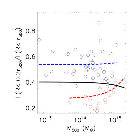
Figure 3: X-ray core-to-$r_{500}$ luminosity fraction versus dynamical mass for the CC (blue) and NCC (red) clusters. The curves show the regression fits for all (black), CC (blue) and NCC (red) clusters, respectively. There is no obvious dependence considering the observed scatter.

Figure 5: Bias (solid curves) and dispersion (dashed curves) of the redshift (left panel) and dynamical mass (right panel) measurements in the 10zs setup from the input cluster values versus input number of cluster galaxies. The curves are smoothed with a boxcar average of the specified width of 11 to avoid spikes due to under-sampling for a few clusters. Note that $n_{\rm gal}$ is the input number of galaxies and the output number of galaxies is always 10.

Figure 8: Bias (solid curves) and dispersion (dashed curves) of the redshift measurements in the 05zs setup from the input cluster values versus input number of cluster galaxies. The curves are smoothed with a boxcar average of the specified width of 11 to avoid spikes due to under-sampling for a few clusters. Note that $n_{\rm gal}$ is the input number of galaxies and the output number of galaxies is always 5.

Appendix A Impact of flux loss of the aperture magnitude

A.1 Fraction of recovered flux

We used a Sérsic profile for the two-dimensional (2D) surface brightness profiles of galaxies (e.g. Peng et al. 2002), $\Sigma(x,y)\propto\exp\left[-\kappa\left(\frac{r_{\rm ell}}{R_{\rm e}}\right)^{1/n}-1\right]$ with $r_{\rm ell}=\left[\left|x\right|^{(c+2)}+\left|\frac{y}{q}\right|^{(c+2)}\right]^{1/(c+2)}$. The parameter $q$ is the ellipticity, and we used its distribution observed in SDSS (Fig. 3 in Hyde & Bernardi 2009, peaked at $\sim$0.8). For a de Vaucouleurs profile, $c=0$, $n=4$, $\kappa=7.67$ for $n=4$, and $\Sigma(x,y)\propto\exp\left[-7.67\left(r_{\rm ell}/R_{\rm e}\right)^{1/4}\right]\;$. Following Bernardi et al. (2007), we computed the effective radius in units of kpc from the $r$-band absolute magnitude for a passive, elliptical galaxy, $\langle\log R_{\rm e}|M_{r}\rangle=-0.681(M_{r}+21)/2.5+0.343$, using the spectral energy distribution template in Maraston et al. (2009).

We assume $1\hbox{$.\!\!^{\prime\prime}$}4$ seeing for SPIDERS and $1\arcsec$ seeing for 4MOST (private communication with T. Dwelly), in which the seeing is better than the given value for 90% of the time. The diameter of the aperture is $\varnothing=2\arcsec$ for SPIDERS and $1\hbox{$.\!\!^{\prime\prime}$}5$ for 4MOST. The resulting flux is computed by integrating the surface brightness profile convolved with the seeing within the aperture. The fractions of recovered flux $f_{\rm synth}$ in the fibers of the SPIDERS and 4MOST surveys are shown in Fig. 9. Our results are consistent with that of the objects classified as “LRG” or “GALAXY” which have spectroscopic redshifts from the BOSS in SDSS DR11.

A.2 Impact on our sampling

For galaxies with an intrinsic magnitude only slightly brighter than the limiting magnitude cut, its aperture magnitude may become fainter than the limiting magnitude when considering flux loss. We inspected this impact on our sampling by comparing the aperture magnitudes of the member galaxies used in the re-sampling with the limiting magnitude cut. Although there is quite a dramatic difference ($\sim$1–1.5 magnitudes) between the total magnitude and the $2\arcsec$ aperture magnitude, we found that the aperture magnitudes of all member galaxies are well above the limiting magnitude cut for the clusters at $z_{\rm in}<0.4$ and $z_{\rm in}=0.8$. This is because the galaxies are much brighter than the limiting magnitude at the low redshift of $z_{\rm in}=0.2$, and the angular sizes of the galaxies are well within the aperture size at the high redshift of $z_{\rm in}=0.8$ such that flux loss plays no role. At redshifts of $z_{\rm in}=$0.4 and 0.6, the aperture magnitude considering flux loss leads to a number of member galaxies fainter than the limiting magnitude in a couple of clusters among 63 clusters in the re-sampling. No more than three out of 63 clusters are affected by the impact of flux loss. We thus consider this effect negligible. Note that the flux loss plays a major role in degrading the spectral quality, which is not part of this study.

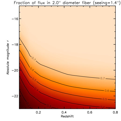
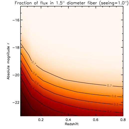
Figure 9: Fractions of recovered flux $f_{\rm synth}$ in the fibers of the SPIDERS (left panel) and 4MOST (right panel) configurations. The $x$-axis and $y$-axis are the galaxy redshift and $r$-band absolute magnitude, respectively.