Analytical parametrization and shape classification of anomalous HH production in the EFT approach - LHCHXSWG-2016-001

Abstract

In this document we study the effect of anomalous Higgs boson couplings on non-resonant pair production of Higgs bosons ($\rm HH$) at the LHC. We explore the space of the five parameters $\kappa_{\lambda}$, $\kappa_{t}$, $c_{2}$, $c_{g}$, and $c_{2g}$ in terms of the corresponding kinematics of the final state, and describe a partition of the space into a limited number of regions featuring similar phenomenology in the kinematics of $\rm HH$ final state. We call clusters the sets of points belonging to the same region; to each cluster corresponds a representative point which we call a benchmark. We discuss a possible technique to estimate the sensitivity of an experimental search to the kinematical differences between the phenomenology of the benchmark points and the rest of the parameter space contained in the corresponding cluster. We also provide an analytical parametrization of the cross-section modifications that the variation of anomalous couplings produces with respect to standard model $\rm HH$ production along with a recipe to translate the results into other parameter-space bases. Finally, we provide a preliminary analysis of variations in the topology of the final state within each region based on recent LHC results.

1 Introduction

The present work stems from the studies we have undertaken to attempt an exhaustive description of the complex parameter space that describes the possible modifications of standard model (SM) production of Higgs boson ($\rm H$) pairs produced by anomalous couplings. The characterization of the phenomenology may be done by considering the shape of density functions of kinematic pseudo-observables fully specifying the production process. By considering kinematical quantities describing $\rm HH$ production at Leading Order (LO), without the inclusion of any initial- or final-state effects nor the decay of the Higgs bosons, one may concentrate on the similarities and the differences produced by distinct physics scenarios, determined by the value of the five anomalous coupling parameters.

While the previous work [1] focused on the qualitative taxonomy of the kinematics induced by di-Higgs production, in this paper we consider mainly the cross section of that process, offering an useful analytical parametrization. In section 2 we provide the parametrization of the Lagrangian density in terms of five anomalous coupling parameters. In section 3 we recall the results of our clustering procedure, and discuss the properties of the identified benchmarks and the intra-cluster variability. In particular the clustering procedure is compared to the first experimental results from the LHC. In section 4 we derive the analytical parametrization of the cross section, discuss its precision, and offer a recasting recipe to use the formula in other bases.

2 Higgs boson pair production by gluon-gluon fusion

In the context of Beyond the Standard Model (BSM) theories, di-Higgs production in gluon-gluon fusion can be described to leading approximation with the Lagrangian [2]

$$\begin{split}{\cal L}_{\rm H}=&\frac{1}{2}\partial_{\mu}\,\rm H\partial^{\mu}\rm H-\frac{1}{2}m_{\rm H}^{2}\rm H^{2}-{\kappa_{\lambda}}\,\lambda_{SM}\nu\,\rm H^{3}\\ &-\frac{m_{t}}{v}(v+{\kappa_{t}}\,\rm H+\frac{c_{2}}{\nu}\,\rm HH)\,(\bar{t_{L}}t_{R}+h.c.)+\frac{1}{4}\frac{\alpha_{s}}{3\pi\nu}(c_{g}\,\rm H-\frac{c_{2g}}{2\nu}\,\rm HH)\,G^{\mu\nu}G_{\mu\nu}\,,\end{split}$$ (1)

where $\nu=246\,$GeV is the vacuum expectation value of the Higgs field. This Lagrangian includes five parameters: the deviation of the Higgs boson trilinear coupling $\lambda$ (top Yukawa coupling $y_{t}$) from its SM value $\lambda_{SM}$ ($y_{t,SM}=\sqrt{2}m_{t}/v$) quantified by $\kappa_{\lambda}\equiv\lambda/\lambda_{SM}$ ($\kappa_{t}\equiv y_{t}/y_{t}^{\rm SM}$), as well as the coefficients of three pure BSM operators which describe the contact interaction between two Higgs bosons and two top quarks ($c_{2}$), and the Higgs boson contact interaction with one ($c_{g}$) and two gluons ($c_{2g}$). In the Effective Field Theory (EFT) description, modifications of the interactions between the Higgs boson and the other SM fields are generated by higher-dimensional operators, which after electroweak symmetry breaking induce the couplings above. While assuming a linear realization of the SM gauge symmetry, i.e., assuming the H boson as part of a weak doublet, leads to relations between these couplings (in the case of a linear realization with dimension-6 operators, we get $c_{2g}=−c_{g}$, see Ref. [3]), those are lifted in the non-linear realization. We do not consider a possible enhanced coupling of the Higgs boson with bottom quarks, which are already constrained experimentally [4].

Five Feynman diagrams can be constructed from the above Lagrangian (see Fig. 1), each corresponding to a matrix element associated to different combinations of BSM and SM-like parameters and different properties of the $\rm HH$ final state.

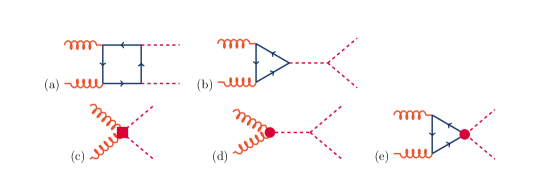
Figure 1: Generic Feynman diagrams that contribute to $\rm HH$ production via gluon-gluon fusion at leading order. Diagrams (a) and (b) correspond to SM-like processes, while diagrams (c), (d) and (e) include pure BSM vertices: (c) and (d) describe contact interactions between the $\rm H$ boson and gluons, and (e) exploits the contact interaction of two $\rm H$ bosons with top quarks.

3 Kinematic clustering

3.1 Clustering procedure

An important consequence of the introduction of the five BSM parameters in the Lagrangian provided in Eq. (1), in addition to the modification of the overall Higgs boson pair-production cross section, is the generation of significant modifications of the kinematic properties of the final state with respect to the pure SM process. The experimental exploration of the five-dimensional model space is by no means trivial, as the optimization of the search strategy for the $\rm HH$ signal depends significantly on the investigated parameter space point. In order to address this problem, we designed a clustering procedure to group regions of parameter space which can be probed by the same search. In the spirit of this approach, analyses would optimize their selection for a model (a benchmark) chosen to represent at best the kinematic characteristics of the corresponding region. The benchmarks resulting from the clustering procedure are summarized in this note; for implementation details the reader is referred to Ref. [1]. We recall below the basic ideas of our procedure.

The $gg\rightarrow\rm HH$ production is a $2\rightarrow 2$ process. In the center-of-mass reference frame the kinematic properties of the final state can be fully characterized by two variables: the invariant mass of the two Higgs bosons $m_{\rm HH}$ and the polar angle of one of the bosons in the center-of-momentum frame $|\cos\theta^{*}|$. At leading order, all other observables describing the final state have no connection to the structure of the Lagrangian density from Eq. 1. The kinematic properties of each EFT point can then be characterized by estimating the two-dimensional probability density function of $m_{\rm HH}$ and $|\cos\theta^{*}|$. By using a suitable test statistic sensitive to the shape differences of the two-dimensional density function, one may quantify the kinematic differences between different model points in the five-dimensional phase-space. The value of the test statistic may then be used to group the models that are kinematically most similar. This procedure is referred to as cluster analysis and a group of models as a cluster. The employed test statistic was a likelihood ratio based on Poisson counts in $m_{\rm HH}-|\cos\theta^{*}|$ histograms; the clustering was performed through a hierarchical agglomerative technique.

The clustering procedure was applied to a set of models corresponding to a fine scan in several parameter space directions. The investigated range of the parameters was decided by taking into account the current experimental constraints. In particular, the parameters were allowed to vary as $|\kappa_{\lambda}|\leq$ 15, $\kappa_{t}\subset[0.5,2.5]$, $|c_{2}|\leq$3 and $(|c_{g}|,|c_{2g}|)\leq 1$, where $\kappa_{t}$ and $c_{2}$ feature a step size of O(0.5) and $\kappa_{\lambda}$ is varied in O(1) steps. The granularity of the scan in $c_{g}$ and $c_{2g}$ is 0.2. To have a better accuracy in the points of minimal di-Higgs production cross section, where the changes in kinematics are particularly strong, we increased the density of scanned points in the corresponding regions. This resulted in a total of 1507 inspected points, distributed with a variable binning within the boundaries quoted above. The simulations were performed with the Madgraph_aMC@NLO version 2.2.1 Monte Carlo (MC) simulation package [5], using the model provided by the authors of [6], were the loop factors including the full $m_{t}$ dependence are calculated on an event-by-event basis with a Fortran routine. The PDF set used was NNPDF23LO1 [7] and the factorization and renormalization scale considered were $\sqrt{\hat{s}}=m_{\rm HH}$. The relevant input masses were $m_{\rm H}$ = 126 GeV and $m_{t}$ = 173.18 GeV.

The cluster analysis leads to the division of the 1507 inspected points into 12 groups. Each group displays similar kinematic characteristics, and clear differences compared with members of the other groups. For each cluster a benchmark is defined as the sample most similar to all the others in the cluster, where the similarity metric is the one given by the test statistic. The numerical details are provided later in sub-section 3.3.

3.2 Outliers

The benchmarks are chosen to capture well the main features of the cluster kinematics. Nevertheless some of the cluster members still exhibit residual differences with respect to the benchmark. These intra-cluster differences could lead to limited deviations in the experimental signal efficiencies. If the analysis has a sufficient resolution to resolve those differences we propose here a simple approach to select six extreme cases (referred to as outliers) within each cluster, which can tentatively be used to evaluate the possible variation of experimental efficiencies within a cluster. If the analyzers want to preserve the simplifications offered by the cluster approach we recommend to fully simulate (generate and propagate through the experimental apparatus) only the benchmark and obtain the outliers through an event-by-event reweighing procedure in the $m_{\rm HH}-|\cos\theta^{*}|$ space. The results (for example limits) shall be then presented for the benchmark and benchmark reweighted to the outliers. The weights may be easily estimated at generator level.

The $m_{\rm HH}$ distribution features the largest intra-cluster variation and it is likely the most important distribution for experimental analyses. We define therefore the outliers as subset of samples that envelope all the other samples of the cluster in three mass points $m_{\rm HH\,,1}\,\equiv$ 270 GeV, $m_{\rm HH\,,2}\,\equiv$ 400 GeV and $m_{\rm HH\,,3}\,\equiv$ 600 GeV, applied to a histogram with 20 GeV wide bins. The first and last mass points are intended to catch the analysis sensitivity to threshold region ($m_{\rm HH}\approx 2m_{\rm H}$) and energy-tail modifications. The intermediate mass point is close to the typical valley found in the distribution due to a cancellation between the different diagrams, and it is intended to catch the analyses sensitivity to short-distance fluctuations in shape. Figure 2 (top) shows an example of the di-Higgs mass distribution for cluster 3 with the outliers. In Fig. 2 (bottom) we provide the $p_{\rm T,H}$ and $|\cos\theta^{*}|$ spectra with the same outliers. One may observe that the choice of outliers in $m_{\rm HH}$ is also reasonably valid for the two other distributions.

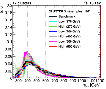
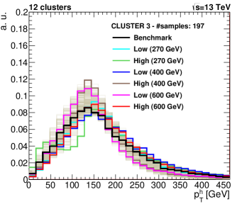
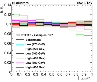
Figure 2: The $m_{\rm HH}$ (top left), $p_{\rm T,H}$ (top right) and $|\cos\theta^{*}|$ (bottom) distributions for the members of cluster 3. The benchmark (in black color) and corresponding outliers (colored lines) are highlighted. The three mass regions are indicated by vertical dashed lines.

3.3 Results

The list of benchmarks is given in Table 1. We recommend the 12 benchmarks listed there to be the parameter space points targeted by experimental searches, in addition to the SM point. Fig. 3 shows the $m_{\rm HH}$ spectra for all the clusters together with the outliers, while Table 2 provides the parameters of all the 72 outliers.

Benchmark	$\kappa_{\lambda}$	$\kappa_{t}$	$c_{2}$	$c_{g}$	$c_{2g}$
1	7.5	1.0	-1.0	0.0	0.0
2	1.0	1.0	0.5	-0.8	0.6
3	1.0	1.0	-1.5	0.0	-0.8
4	-3.5	1.5	-3.0	0.0	0.0
5	1.0	1.0	0.0	0.8	-1.0
6	2.4	1.0	0.0	0.2	-0.2
7	5.0	1.0	0.0	0.2	-0.2
8	15.0	1.0	0.0	-1.0	1.0
9	1.0	1.0	1.0	-0.6	0.6
10	10.0	1.5	-1.0	0.0	0.0
11	2.4	1.0	0.0	1.0	-1.0
12	15.0	1.0	1.0	0.0	0.0
SM	1.0	1.0	0.0	0.0	0.0

Table 1: Parameter values of the final benchmarks selected by the clustering procedure [1]. The third cluster is the one that contains the SM sample (defined by $\kappa_{\lambda}$ = $\kappa_{t}$ =1, $c_{2}$ = $c_{g}$ = $c_{2g}$ = 0).

Three of the clusters have benchmarks that do not obey the linear EFT relation, however this does not present a problem for the interpretation of the results, assuming the latter. The phenomenological properties of parameter points within these clusters that belong to the linear realization of EWSB are still well approximated by the corresponding benchmarks.

Relevant properties of those three clusters are described below:

• In the scan we performed, Cluster 2 does not have representatives in the linear theory. The $m_{\rm HH}$ extends above the TeV scale - therefore particular caution should be taken when interpreting the experimental results derived for the corresponding benchmark in the EFT (see Fig. 3).

• Cluster 3 includes the SM point and a large fraction of the points where only $\kappa_{\lambda}$ and $\kappa_{t}$ are modified, while the coefficients related to purely BSM operators are constrained to 0.

• Cluster 5 exhibits a doubly peaked structure in $m_{\rm HH}$, corresponding to maximal interference pattern and associated with regions of minimal cross sections, which also includes points of the linear case (see Fig. 3).

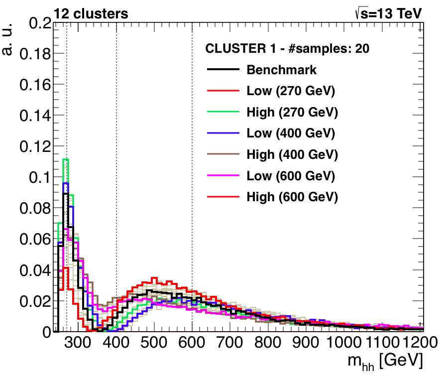
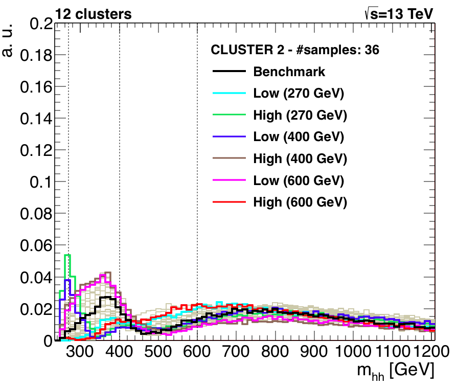
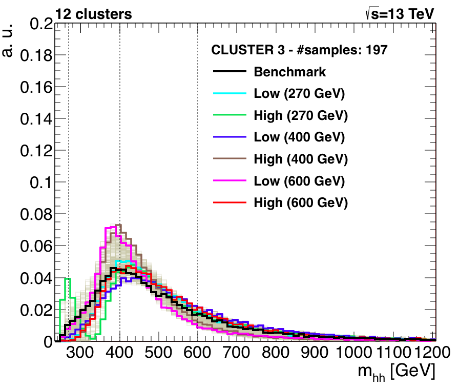
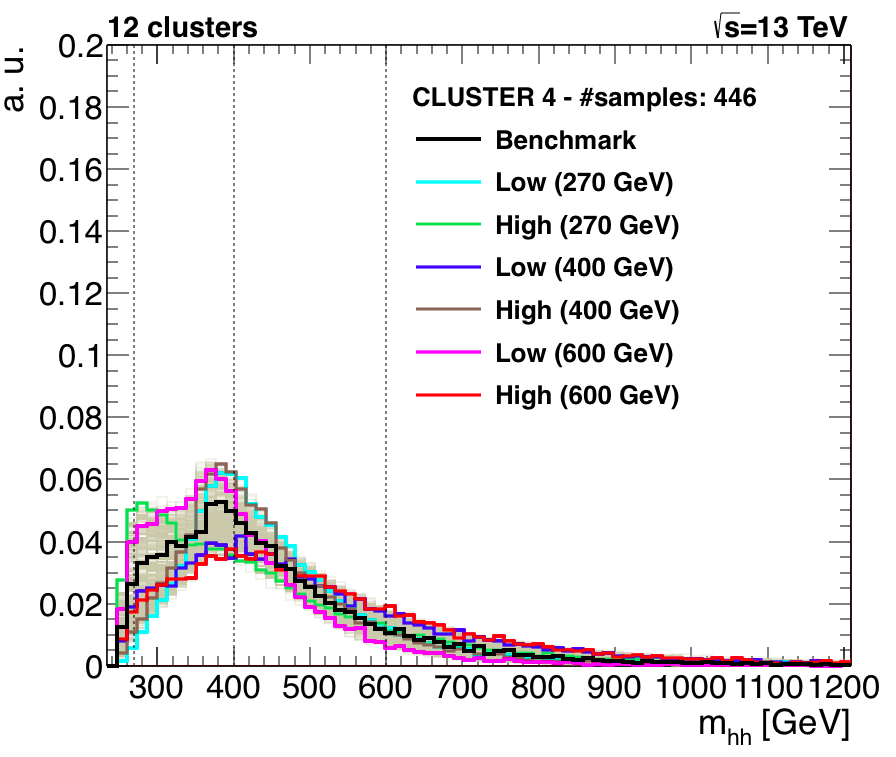
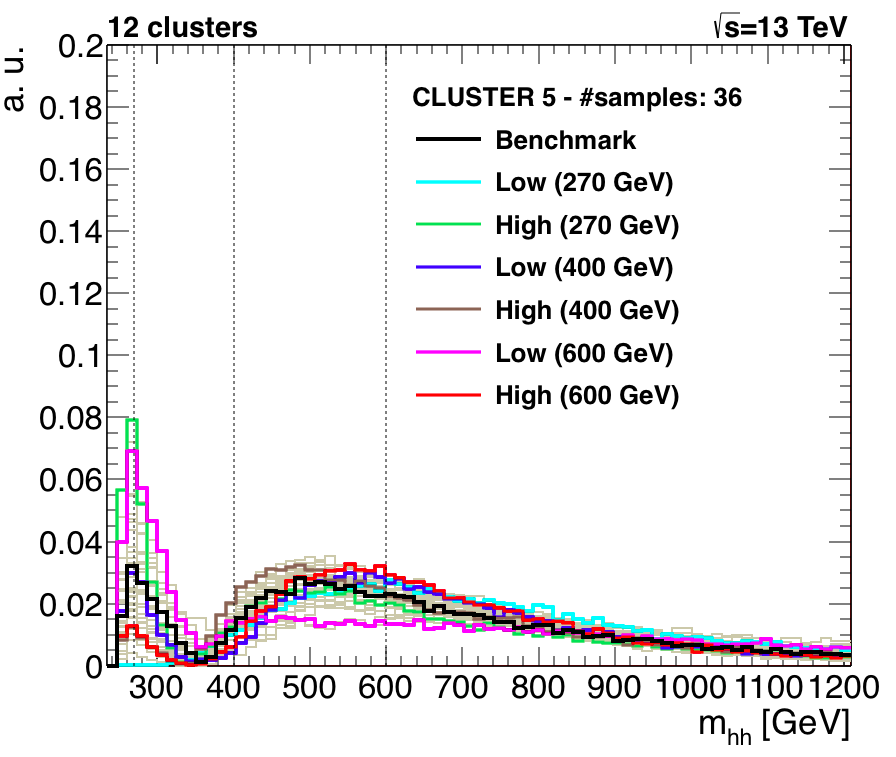
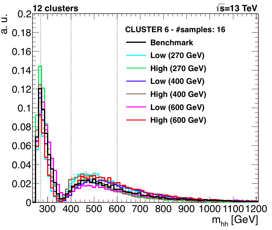
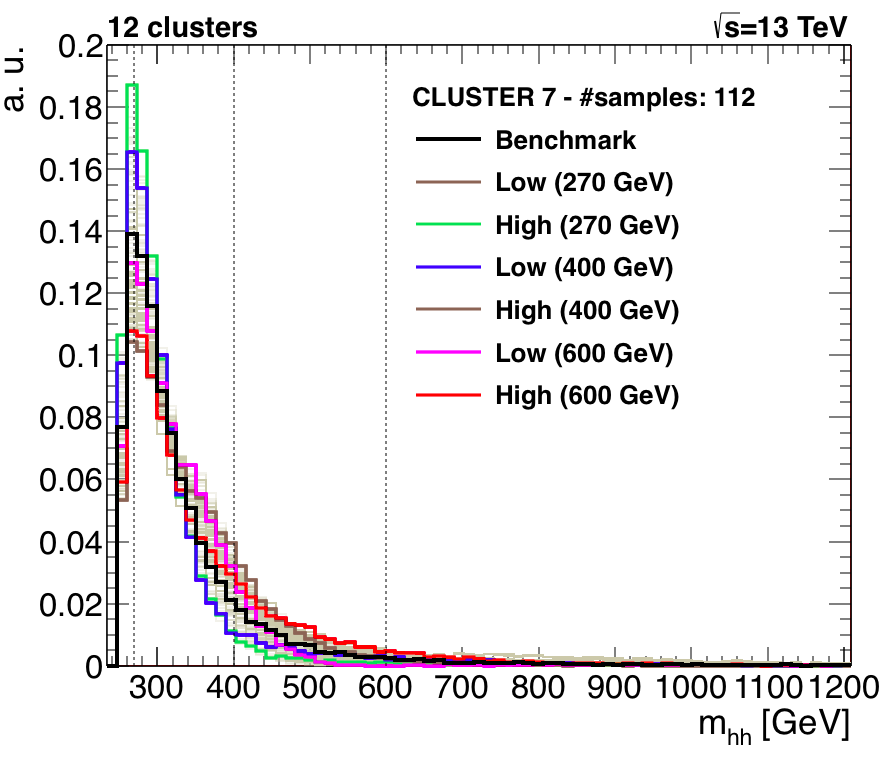
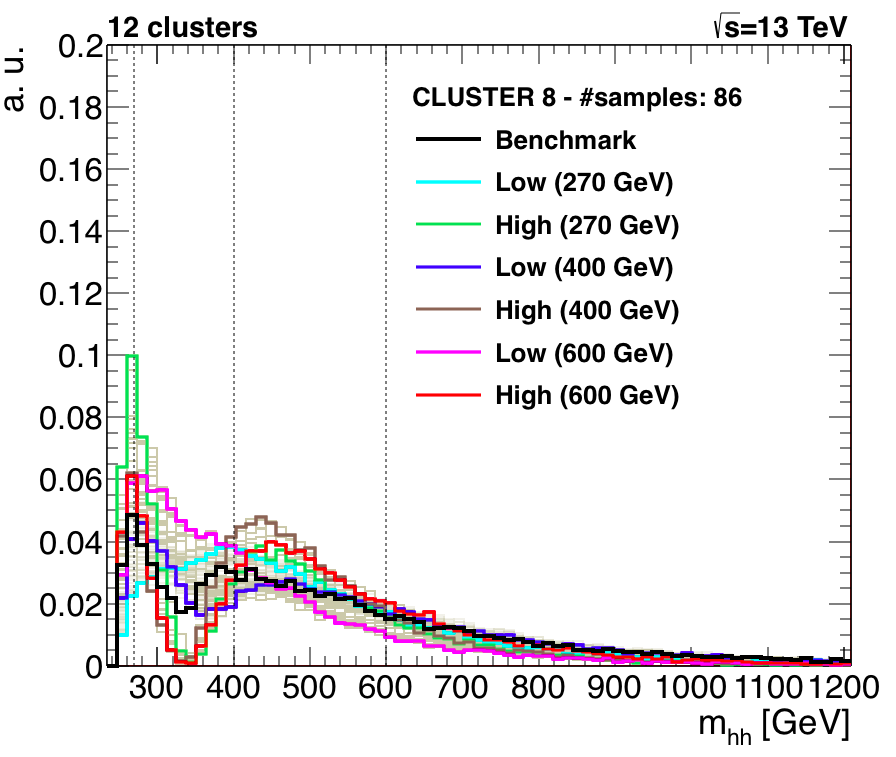
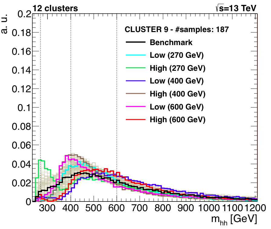
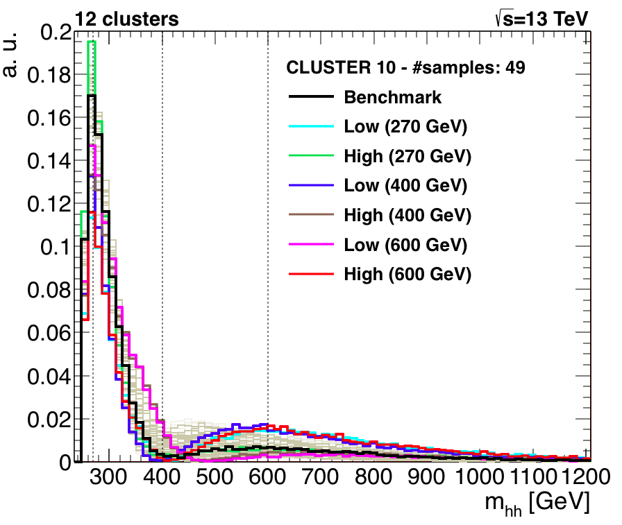
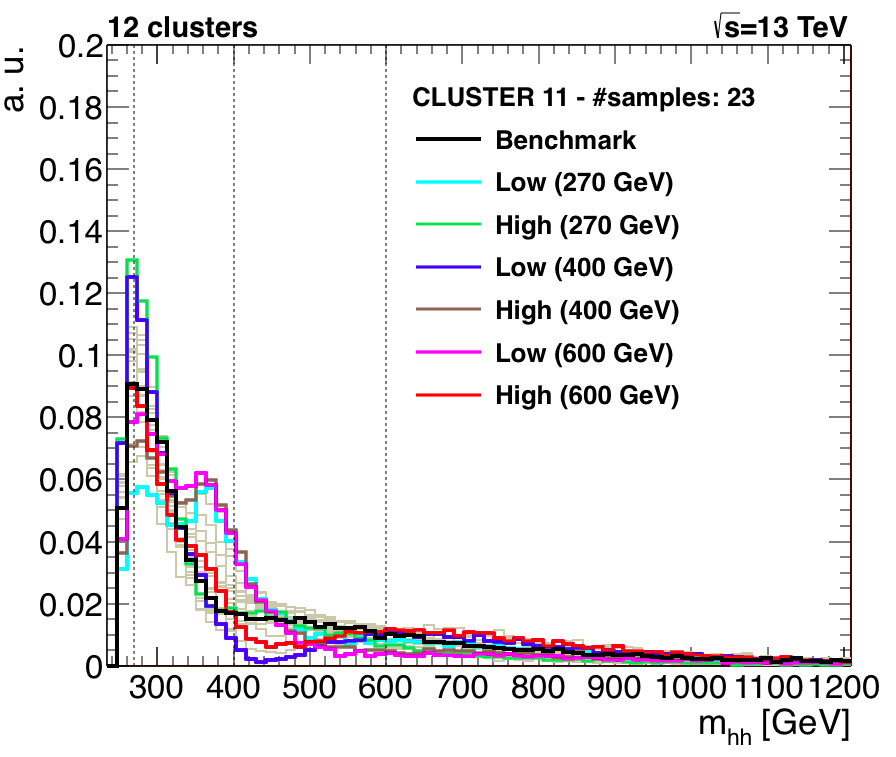
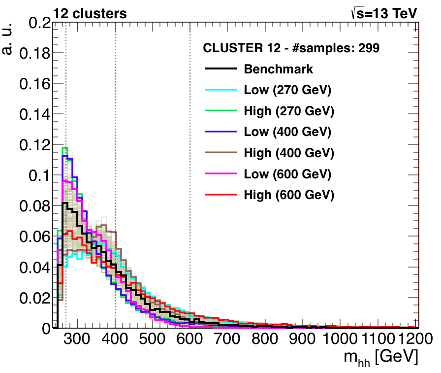
Figure 3: The $m_{\rm HH}$ distributions for the 12 clusters. The benchmark (in black color) and corresponding outliers (colored lines) are highlighted. The mass points $m_{\rm HH}^{1}$, $m_{\rm HH}^{2}$ and $m_{\rm HH}^{3}$ are indicated by vertical dashed lines.

Cluster 1					Cluster 2					Cluster 3
$\kappa_{\lambda}$	$\kappa_{t}$	$c_{2}$	$c_{g}$	$c_{2g}$	$\kappa_{\lambda}$	$\kappa_{t}$	$c_{2}$	$c_{g}$	$c_{2g}$	$\kappa_{\lambda}$	$\kappa_{t}$	$c_{2}$	$c_{g}$	$c_{2g}$
15.0	1.0	-3.0	0.0	0.0	1.0	1.0	0.5	1.0	0.8	-10.0	0.5	3.0	0.0	0.0
15.0	1.0	-3.0	0.0	0∗	1.0	1.0	0.5	0.8	0.8	5.0	1.5	-2.0	0.0	0.0
1.0	1.0	0.5	1.0	0.4	1.0	1.0	0.5	-0.6	0.4	2.4	1.0	-0.5	0.0	0.0
1.0	1.0	0.5	1.0	0.2	1.0	1.0	0.5	-0.8	0.4	2.4	2.0	1.0	0.0	0.0
15.0	1.5	-3.0	0.0	0.0	1.0	1.0	0.5	-1.0	0.8	2.4	2.5	1.0	0.0	0.0
-10.0	0.5	1.0	0.0	0.0	1.0	1.0	0.5	-1.0	1.0	1.0	2.5	1.5	0.0	0.0
Cluster 4					Cluster 5					Cluster 6
$\kappa_{\lambda}$	$\kappa_{t}$	$c_{2}$	$c_{g}$	$c_{2g}$	$\kappa_{\lambda}$	$\kappa_{t}$	$c_{2}$	$c_{g}$	$c_{2g}$	$\kappa_{\lambda}$	$\kappa_{t}$	$c_{2}$	$c_{g}$	$c_{2g}$
5.0	2.0	3.0	0.0	0.0	5.0	1.0	0.0	-0.6	0.6	10.0	2.5	-2.0	0.0	0.0
1.0	1.5	3.0	0.0	0.0	1.0	1.0	0.5	1.0	0.6	5.0	1.0	-0.5	0.0	0.0
1.0	1.0	2.0	0.0	-0.4	1.0	1.0	0.0	0.2	-0.8	7.5	1.5	-1.0	0.0	0.0
1.0	1.0	0.0	0.4	0.6	1.0	1.0	0.5	-1.0	0.2	2.4	1.0	0.0	0.4	-0.4
1.0	1.0	0.0	-0.2	0.4	-2.4	1.5	2.0	0.0	0.0	5.0	2.5	1.0	0.0	0.0
-2.4	1.0	0.0	-0.6	0.6	-2.4	1.0	1.0	0.0	0.0	5.0	1.75	0.0	0.0	0.0
Cluster 7					Cluster 8					Cluster 9
$\kappa_{\lambda}$	$\kappa_{t}$	$c_{2}$	$c_{g}$	$c_{2g}$	$\kappa_{\lambda}$	$\kappa_{t}$	$c_{2}$	$c_{g}$	$c_{2g}$	$\kappa_{\lambda}$	$\kappa_{t}$	$c_{2}$	$c_{g}$	$c_{2g}$
10.0	2.5	2.0	0.0	0.0	7.5	2.5	-1.0	0.0	0.0	10.0	0.5	-2.0	0.0	0.0
15.0	0.5	0.0	0.0	0.0	3.5	2.0	0.5	0.0	0.0	1.0	1.0	0.0	-0.2	-0.4
15.0	0.5	0.0	0.0	0∗	5.0	2.0	0.0	0.0	0.0	1.0	1.0	0.0	-1.0	-0.6
-12.5	0.5	0.5	0.0	0.0	7.5	2.0	3.0	0.0	0.0	1.0	1.0	0.5	-1.0	0.0
5.0	1.0	0.0	-0.2	0.2	1.0	1.0	0.5	0.4	0.0	-5.0	1.0	2.0	0.0	0.0
7.5	1.75	0.0	0.0	0.0	1.0	1.0	1.5	0.4	-0.4	1.0	1.0	0.5	0.4	0.2
Cluster 10					Cluster 11					Cluster 12
$\kappa_{\lambda}$	$\kappa_{t}$	$c_{2}$	$c_{g}$	$c_{2g}$	$\kappa_{\lambda}$	$\kappa_{t}$	$c_{2}$	$c_{g}$	$c_{2g}$	$\kappa_{\lambda}$	$\kappa_{t}$	$c_{2}$	$c_{g}$	$c_{2g}$
5.0	1.0	0.0	-0.4	0.4	5.0	2.0	1.0	0.0	0.0	3.5	0.75	0.5	0.0	0.0
-7.5	0.5	0.5	0.0	0.0	-2.4	2.5	3.0	0.0	0.0	-5.0	1.0	-1.0	0.0	0.0
-12.5	1.5	3.0	0.0	0.0	-3.5	2.0	2.0	0.0	0.0	-2.4	2.5	1.0	0.0	0.0
15.0	1.0	-2.0	0.0	0.0	-3.5	2.5	3.0	0.0	0.0	7.5	1.0	0.0	0.6	-0.6
-5.0	0.5	0.5	0.0	0.0	-5	2.0	3.0	0.0	0.0	7.5	1.5	0.5	0.0	0.0
-10.0	1.0	2.0	0.0	0.0	-10.0	1.5	3.0	0.0	0.0	-15.0	2.5	3.0	0.0	0.0

Table 2: The parameter space coordinates of the outliers of the clusters whose benchmarks are in Table 1.

3.4 Experimental results from LHC Run I data taking period

Recently both ATLAS and CMS collaborations performed searches for the non resonant production of Higgs boson pairs with 8 TeV LHC data [8, 9, 10, 11]. The ATLAS collaboration considered only the SM-like kinematics for the signal. The best upper limit of $\sigma_{\rm HH}<0.69$ pb is obtained in Ref. [9] as a results of a combination of the four channels $\rm HH\to\tau\tau\,b\bar{b}$, $\rm HH\to\gamma\gamma\,b\bar{b}$, $\rm HH\to b\bar{b}\,b\bar{b}$ and $\rm HH\to\gamma\gamma\,WW$. For the same hypothesis, the CMS collaboration provides a limit of $\sigma_{\rm HH}<0.71$ pb based on the results from the $\rm HH\to\gamma\gamma\,b\bar{b}$ channel [11].

Reference [11] pushes further the exploration of the BSM parameter space for non-resonant $\rm HH$ production, by varying a subset of the parameter space, given by $\kappa_{\lambda},\kappa_{t}$ and $c_{2}$. All in all, a grid of 124 points was generated. First a scan of $\kappa_{\lambda}$ was performed: $\kappa_{\lambda}=\pm$20, $\pm$15, $\pm$10, $\pm$5, 2.4, 1 (the SM point) and 0. In addition eight two-dimensional scans were done in the plane $(c_{2},\kappa_{t})$, for fixed values of $\kappa_{\lambda}=\pm$20, $\pm$15, $\pm$10, 1 and 0. In those, $c_{2}=\pm$3, $\pm$2, 0 and $\kappa_{t}=$ 0.75, 1, 1.25 were considered. One may notice that the scan in the $\kappa_{t}$ variable covers a smaller range than the scan that defined the clusters, but with a finer granularity.

The signals are searched for in two regions of $m_{\rm HH}$, $<350$ and $m_{\rm HH}>350$ GeV, optimized to maximize the sensitivity for the SM-like search. The observed limits on $\sigma_{\rm HH}$ span between 1.36 pb and 4.42 pb depending on the point of the phase-space. By itself this result shows the importance of the kinematics of the BSM non-resonant production.

The particularity of the $\rm HH\to\gamma\gamma\,b\bar{b}$ channel is to provide an excellent reconstruction of $m_{\rm HH}$ with a resolution of $10-20$ GeV and a rather constant signal efficiency for $250<m_{\rm HH}<1000$ GeV varying between 20% and 30%. Therefore this channel is well suited to resolve the details of the $m_{\rm HH}$ spectrum and to challenge the cluster approach. This is what we discuss in the following by applying the clustering technique to the analyzed parameter space.

From the 124 parameter space points for which we have experimental limits, only $N_{\rm samples}=31$ coincide exactly with any of the parameter space points used to determine the clusters. However we note that other $N_{\rm samples}=22$ extra points lie in between points that belong to the same cluster, while the gradient of cross section between them is smooth. This allows one to tag those intermediate points as belonging to the same cluster. As an example we show in Fig. 4 the distribution of the points used for the cluster definition in two-dimensional scans in $(c_{2},\kappa_{t})$, for fixed values of $\kappa_{\lambda}=\pm$ 15 and $\pm$10. Following the above defined algorithm the point $(\kappa_{\lambda},\kappa_{t},c_{2})=(15,1.25,-2)$ is assigned as belonging to cluster 10. Similarly the point $(\kappa_{\lambda},\kappa_{t},c_{2})=(15,0.75,-2)$ is not assigned to any cluster.

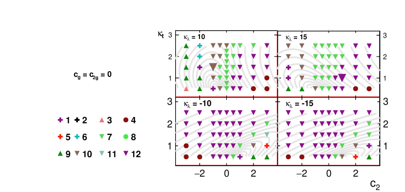
Figure 4: Distribution of points in the $c_{2}\times\kappa_{t}$ plane for different values of $\kappa_{\lambda}$ when $(c_{g},\,c_{2g})=(0,0)$. Circles describe clusters whose benchmark has Higgs boson $p_{T}$ ($p_{\rm T,H}$) peaking around 100 GeV. Downward-pointing triangles describe clusters where $p_{\rm T,H}$ is peaking around 50 GeV or less, while upward-pointing triangles describe ones with $p_{\rm T,H}$ peaking around 150 GeV or more. Finally, crosses describe clusters that show a double peaking structure in the $p_{\rm T,H}$ distribution. Larger markers indicate benchmark points. The gray lines correspond to iso-contours of constant cross section $\sigma_{\rm HH}$. See Fig. 8 in Ref. [1] for more details.

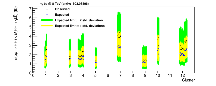
Figure 5: Experimental limits from $\rm HH\to\gamma\gamma\,b\bar{b}$ search performed by the CMS collaboration [11], organized by clusters following the procedure described in the text. The blue points correspond to the 95% CL expected limits, while the green and yellow bands visualize one and two standard deviations around the latter.

In Fig. 5 we show a total of 53 experimental limits at 95% CL, organized by clusters. Unfortunately not all the clusters are equally populated and the statistics ranges between 0 and 19 samples. Still we have enough information to derive the first conclusions.

Table 3 contains the mean values of the expected and observed experimental limits for each cluster and the standard deviations, defined with respect to the mean value. The same information is displayed in Fig. 6, for the observed limits only. As expected the largest limits correspond to threshold-like clusters, for instance cluster 7 and cluster 10. Clusters 4 and 12 seem to exhibit two sub-clusters each. In the figure we also include the values of the medians. This estimator is less affected by the outliers than the mean. We observe that mean and median are close to each other in most cases.

As the observed limits are more susceptible to small data fluctuations their variance is bigger than the spread of the expected limits. The standard deviation derived for each cluster should be taken with care, as the parameter space scan in Ref. [11] was not done in a systematic way regarding the signal kinematic properties. For most of the clusters the relative size of the standard deviation does not exceed 5-10%. For cluster 1 and 10 it increases up to 20%. In Fig. 7 we show the comparison of the $m_{\rm HH}$ distributions. We observed as expected that the largest difference in limits corresponds to the largest difference in shapes. Therefore reweighting the benchmark to the outliers is an important element of an experimental analysis using this cluster technique.

By eye we see that the intra-cluster variance ($V_{\rm Intra,i}$) is smaller than the variance of limits between clusters (inter-cluster variance $V_{\rm Inter,i}$). To provide a more quantitative estimate of this phenomenon we use the Fisher-Snedecor test quite commonly used in biology for example to assess the compatibility of two medical tests. It is implemented via

$${\rm p}\mbox{-}{\rm value}={\rm TMath::FDist}(V_{\rm Inter}/V_{\rm Intra,i},N_{clus},\#{\rm samples}).$$ (2)

It uses the ratio of inter-cluster variance and intra-cluster variance for each cluster. The number of degrees of freedom of the numerator is assumed to be $N_{clus}=8$ and the denominator is the number of samples. The output of this function is a p-value on the hypothesis that both variances are statistically compatible. The results are provided in Table 3. We observe that the clustering procedure is successful to reduce the variance of the phase-space and identify groups with similar experimental behavior in the complex phase-space of $\rm HH$ production final state.

Benchmark	1	3	4	5	7	9	10	12	All
# samples	3 (1)	3 (2)	13 (4)	2 (1)	8 (5)	9 (6)	5 (2)	19 (10)	8 Means
Obs. Mean (pb)	1.92	1.75	1.87	1.34	4.08	1.39	3.63	2.69	2.33
$\sqrt{\mbox{Variance}}$ (pb)	0.55	0.11	0.22	0.03	0.19	0.05	0.53	0.41	1.03
FS p-value	6e-02	3e-05	6e-07	7e-07	5e-06	1e-12	4e-02	5e-04
Exp. Mean (pb)	1.51	1.52	1.61	1.1484	2.84	1.18	2.39	2.18	1.80
$\sqrt{\mbox{Variance}}$ (pb)	0.30	0.08	0.15	0.005	0.09	0.04	0.32	0.25	0.61
FS p-value	4e-02	8e-05	3e-06	4e-09	5e-07	3e-11	4e-02	6e-04

Table 3: Mean and standard deviations of the expected and observed limits for the 8 clusters analyzed in the $\rm HH\to\gamma\gamma\,b\bar{b}$ search performed by CMS collaboration. The label ”# samples” denotes the number of samples identified per cluster. The number in parentheses indicates how many of these were identified to be in the cluster from interpolation, as described in the text. The last column shows the total unweighted mean and the associated standard deviation between the means of the 8 clusters. The Fisher-Snedecor p-values are also provided.

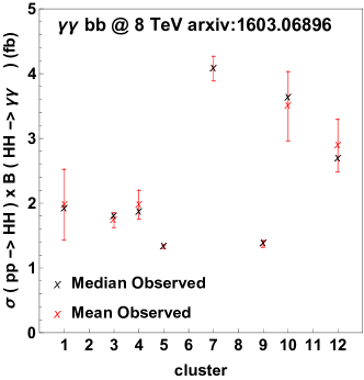
Figure 6: Experimental limits from the $\rm HH\to\gamma\gamma\,b\bar{b}$ analysis performed by the CMS collaboration [11], organized by clusters; see text for details.

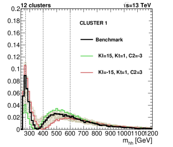
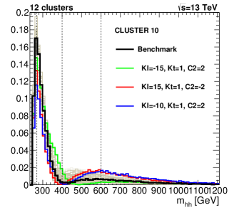
Figure 7: The $m_{\rm HH}$ distribution of the samples in cluster 1 and 10. The benchmark (black line) is compared with the points studied by [11] (bold color red and blue lines) that coincide with those considered in [1].

4 Analytical parametrization of the cross section

The effect of anomalous couplings on the di-Higgs production cross section can be written in the form of a ratio $R_{\rm HH}$ between the cross section of the BSM model and the SM cross section using a vector of numerical coefficients $\mathbf{A}=[A_{1},...,A_{15}]$:

$$\begin{split}R_{\rm HH}\equiv\frac{\sigma_{\rm HH}}{\sigma_{\rm HH}^{\rm SM}}\overset{LO}{=}&A_{1}\,\kappa_{t}^{4}+A_{2}\,c_{2}^{2}+(A_{3}\,\kappa_{t}^{2}+A_{4}\,c_{g}^{2})\,\kappa_{\lambda}^{2}+A_{5}\,c_{2g}^{2}\\ &+(A_{6}\,c_{2}+A_{7}\,\kappa_{t}\kappa_{\lambda})\kappa_{t}^{2}+(A_{8}\,\kappa_{t}\kappa_{\lambda}+A_{9}\,c_{g}\kappa_{\lambda})c_{2}\\ &+A_{10}\,c_{2}c_{2g}+(A_{11}\,c_{g}\kappa_{\lambda}+A_{12}\,c_{2g})\,\kappa_{t}^{2}\\ &+(A_{13}\,\kappa_{\lambda}c_{g}+A_{14}\,c_{2g})\,\kappa_{t}\kappa_{\lambda}+A_{15}\,c_{g}c_{2g}\kappa_{\lambda}\,.\end{split}$$ (3)

To obtain the total cross section for each point in the parameter space described by the couplings of the Lagrangian (1), we recommend to use the relation:

$$\sigma_{\rm HH}=\sigma_{\rm HH,NNLO+NNLL}^{\rm SM}\cdot R_{\rm HH}\,,$$ (4)

where $\sigma_{\rm HH,NNLO+NNLL}^{\rm SM}$ is the state-of-the-art SM cross section, calculated including QCD corrections at Next-to-Next-to-Leading Order (NNLO) and matched to Next-to-Next-to-Leading Log resummations (NNLL), this result can be found on [12]. It was obtained by several independent calculations [13, 14, 15, 16, 17, 18, 19].

4.1 Definition of the procedure to extract the coefficients

The coefficients $\mathbf{A}$ can be extracted from a fit to the cross sections estimated by MC integration in different points of the BSM parameter space. The choice of those input points is critical in order to obtain an accurate parametrization. One needs to assure a sufficient sensitivity of the $\rm HH$ cross section to all coefficients in Eq. (3) and at the same time scan a broad enough range such as to obtain a control on the error in the fit and its internal consistency. To this end, we explore the various directions in the parameter space by studying two-dimensional (2D) planes, starting with the SM-like plane $(\kappa_{\lambda},\kappa_{t})$ and the $(c_{2},\kappa_{t})$ plane. We follow the relation between the Higgs-gluon contact interactions that comes from the linear dimension-6 EFT formalism ($c_{g}=-c_{2g}$) to select two other 2D planes $(c_{2},c_{g})$ and $(\kappa_{\lambda},c_{g})$. Finally, the ambiguities from the EFT relation are removed by scanning the planes $(c_{g},c_{2g})$ and $(c_{2g},c_{2})$. Parameters that are not mentioned here are set to their SM values, such that the SM benchmark point is present in all the two-dimensional subsets of the point set. The final set is composed of 251, 266, 265, 261 and 169 points, corresponding to LHC center-of-mass (CM) energies of 7, 8, 13, 14, and 100 TeV, respectively. We verified that for each CM energy the number of samples is always sufficient to constrain the coefficients with high precision, as shown below.

The components of $\mathbf{A}$ are extracted by maximizing the likelihood simultaneously for all the coefficients, taking into account all the points, i.e., minimizing

$$\log L(\mathbf{A})=\sum_{i\,\subset\,\mbox{event set}}\left(\frac{\sigma_{\rm HH,MC}^{i}-\sigma_{\rm HH}^{i}(\mathbf{A})}{\delta\sigma_{\rm HH,MC}^{i}}\right)^{2}\,,$$ (5)

where $i$ runs over all the points in the set, $\sigma_{\rm HH,MC}^{i}$ is the corresponding cross section calculated by the simulation, $\sigma_{\rm HH}^{i}(\mathbf{A})$ is the cross section in the same parameter space point calculated via Eq. 3 and $\delta\sigma_{\rm HH,MC}^{i}$ is the statistical MC uncertainty assigned to each point. The minimization of $\log L(\mathbf{A})$ is performed with MINUIT and the results are cross-checked with a fit performed with Mathematica.

The cross sections are calculated using the Madgraph_aMC@NLO model also used for the signal shapes. We generate 10,000 events per point $i$. As proton setting we employ the central PDF of the PDF4LHC15_nlo_mc_pdfas [20, 21, 22, 23, 24] set, the strong coupling is taken as $\alpha_{s}(m_{Z})=0.118$, and the factorization and renormalization scales are fixed to $m_{\rm HH}/2$. The input masses are $m_{\rm H}$ = 125 GeV, $m_{t}$ = 173.18 GeV, and $m_{b}$ = 4.75 GeV. Each point is simulated with a different random seed to avoid statistical correlations between the points.

The size of $\delta\sigma_{\rm HH,MC}^{i}/\sigma_{\rm HH,MC}^{i}$ is estimated a posteriori after a first fit by looking on the pulls between the simulated cross sections and the interpolated ones, requiring ${\rm RMS}\approx 1$ for the residuals of the fit. With this procedures we find $\delta\sigma_{\rm HH,MC}^{i}/\sigma_{\rm HH,MC}^{i}=0.03\%$ is a good estimate of the uncertainties at all CM energies.The SM point is a particular case: by definition $R_{\rm HH}(SM)=1$ with no uncertainty. In practice to avoid infinite values in the likelihood we define $\delta\sigma_{\rm HH,MC}^{i=SM}/\sigma_{\rm HH,MC}^{i=SM}\equiv 0.01\%$.

4.2 Fit results

The central values for $\mathbf{A}$ are shown in Table 4. It is not trivial to identify a general trend in the behavior of the coefficients as a function of the CM energy. We may still observe that the coefficients $A_{1}$, $A_{3}$, and $A_{7}$ related to the SM like Feynman diagrams ((a) and (b) in Fig. 1) and their interference term decrease in magnitude with CM. The coefficients related to the pure BSM diagrams $A_{2}$ and $A_{5}$ ((c) and (e) in Fig. 1) in contrary increase, which can be understood from the fact that they correspond to genuinely higher dimensional contributions. The coefficient $A_{4}$ ((d) in Fig. 1) mixing a BSM operator and SM-like one is rather stable. The trend of the other coefficients corresponding to interference terms are more complex to describe. Fig. 8 shows the comparison of the MC cross section with the result of the cross section Formula 3, using the coefficients of Table 4. We display $R_{\rm HH}$ as function of different couplings in sub-spaces of the six planes used to fix the latter formula for the LHC at 13 TeV. The order of magnitude and general behavior of the minima of $R_{\rm HH}$ is very similar for the LHC running at 7-14 TeV. Differences may be observed when considering a large jump from 14 to 100 TeV energy in CM.

Finally, we illustrate in Fig. 9 that, although kinematics and total cross section are correlated on one hand, the same topology can be obtained for points with cross sections that differ by orders of magnitude but, on the other hand, points with the same total cross section can feature very different kinematics.

$\sqrt{s}$	7 TeV	8 TeV	13 TeV	14 TeV	100 TeV
$A_{1}$	2.21	2.18	2.09	2.08	1.90
$A_{2}$	9.82	9.88	10.15	10.20	11.57
$A_{3}$	0.33	0.32	0.28	0.28	0.21
$A_{4}$	0.12	0.12	0.10	0.10	0.07
$A_{5}$	1.14	1.17	1.33	1.37	3.28
$A_{6}$	-8.77	-8.70	-8.51	-8.49	-8.23
$A_{7}$	-1.54	-1.50	-1.37	-1.36	-1.11
$A_{8}$	3.09	3.02	2.83	2.80	2.43
$A_{9}$	1.65	1.60	1.46	1.44	3.65
$A_{10}$	-5.15	-5.09	-4.92	-4.90	-1.65
$A_{11}$	-0.79	-0.76	-0.68	-0.66	-0.50
$A_{12}$	2.13	2.06	1.86	1.84	1.30
$A_{13}$	0.39	0.37	0.32	0.32	0.23
$A_{14}$	-0.95	-0.92	-0.84	-0.83	-0.66
$A_{15}$	-0.62	-0.60	-0.57	-0.56	-0.53

Table 4: Central values for the coefficients entering $R_{hh}$ (Eq. (3)), employing the anomalous couplings parametrization (Eq. 1).

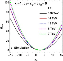
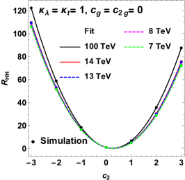
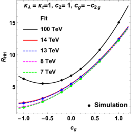
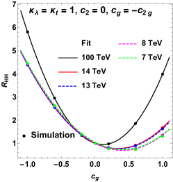
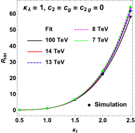
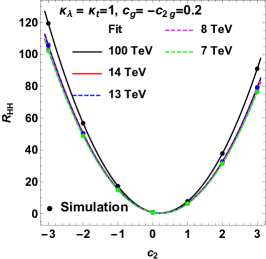
Figure 8: Comparison of the cross sections predicted by Eq. 3 with the MC cross sections for different combinations of parameters.

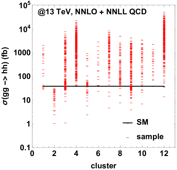
Figure 9: Cross sections for the parameter-space points, depicted by red markers and grouped into 12 clusters. The black horizontal line shows the SM cross section.

4.3 Uncertainties

The different sources of uncertainties considered in this analysis are: statistical uncertainties on the MC samples, uncertainty in QCD parameters (proton PDF and $\alpha_{s}$) as well as missing order uncertainties.

The statistical uncertainties in the cross section for each sample $i$ predicted by MC integration was estimated in Section 4.1 to be 0.03%. The resulting impact on the coefficients $\mathbf{A}$ was observed to be negligible.

The cross section uncertainties due to the different parton distribution functions (PDFs) and $\alpha_{s}$ are obtained following the recommendation for Run 2 provided by Ref. [21]. We use the MC PDF set PDF4LHC15_nlo_mc_pdfas with $N_{\rm rep}=$ 100 replicas and $\alpha_{s}(m_{Z})=0.118$. Moreover, we consider two extra replicas with $\alpha_{s}(m_{Z})=0.1165$ and $\alpha_{s}(m_{Z})=0.1195$.

To estimate the PDF uncertainty in $R_{\rm HH}$ we calculate for a sample $i$ and a replica $j$ the deviation

$$\delta_{\rm PDF}^{i,j}\equiv 1-\frac{R_{\rm HH}^{i,j}}{R_{\rm HH}^{i,CV}}$$ (6)

with respect to the value of the ratio calculated with the central value of PDF4LHC15_nlo_mc_pdfas, $R_{\rm HH}^{i,CV}$. The PDF uncertainty for $i$ is then obtained as

$$\delta_{PDF}^{i}\equiv\sqrt{\frac{1}{N_{rep}-1}\sum_{j=1}^{N_{rep}}(\delta_{PDF}^{i,j})^{2}}.$$ (7)

The $\delta_{\alpha_{S}}^{i}$ uncertainty is estimated as the relative difference between two replicas obtained with modified values of $\alpha_{s}(m_{\rm Z})$: 0.1165 and 0.1195. The total uncertainty on $R_{\rm HH}^{i}$ can finally be obtained as

$$\delta R_{\rm HH}^{i}\equiv\sqrt{(\delta_{\rm PDF}^{i})^{2}+(\delta_{\alpha_{S}}^{i})^{2}}.$$ (8)

The uncertainty due to the QCD parameters related to proton settings in the total cross section is a function of the signal topology. To good approximation, all samples within a cluster probe the same topology. We present in Table 5 the impact of the uncertainties on the 12 benchmarks of Table 1 for different CM energies. We observe that the QCD uncertainties cancel out in the ratio down to a residual few per mill. In consequence, the uncertainty in $R_{\rm HH}$ due to limited MC statistics and QCD parameters are negligible to very good approximation.

Benchmark	1	2	3	4	5	6	7	8	9	10	11	12
$\sqrt{s}$	$\delta R_{\rm HH}^{i}$ (%)
8 TeV	0.1	0.2	0.0	0.1	0.1	0.1	0.2	0.1	0.1	0.2	0.0	0.1
13 TeV	0.1	0.3	0.0	0.0	0.1	0.1	0.2	0.1	0.1	0.2	0.0	0.1
14 TeV	0.1	0.3	0.1	0.0	0.2	0.1	0.2	0.2	0.1	0.2	0.0	0.1
100 TeV	0.3	1	0.2	0.0	0.8	0.2	0.4	0.5	0.5	0.2	0.1	0.3

Table 5: Total theory uncertainty on the ratio $R_{\rm HH}^{i}$ (in %), including PDF and $\alpha_{S}$ variations, for each of the benchmark points $i$ of table 2 and the four center of mass energies we consider. The null entries correspond to points where $\delta R_{\rm HH}^{i}$ is smaller than 0.05%.

Finally, we tried to estimate the impact of the missing orders on $R_{\rm HH}$ calculated at LO. The $K$-factor for the total cross section is found to be fairly flat in the five parameter space directions we scan here when calculated at NLO QCD [26]. Consequently it almost cancels out in $R_{\rm HH}$. The largest observed variation of 5% in the infinite top mass limit appears for the extreme BSM case of a sizable contact interaction among two Higgs bosons and gluons.

This modest value suggests that the theory uncertainties in the total cross section that are due to missing orders can be well approximated by the theory uncertainties assumed for the cross section normalization $\sigma_{\rm HH,NNLO+NNLL}^{\rm SM}$, as recommended in Ref. [12].

We also compared our predictions at LO in a narrow range of variations in the trilinear self-coupling $(\kappa_{\lambda}\in[-1,2])$, to the $R_{\rm HH}$ calculated including QCD corrections up to NNLO and NNLL, which corresponds to the state of the art for the SM calculation [12, 18, 19]. We find the maximum deviation from our predictions to be 6% at a CM energy of 100 TeV at the boundaries of the inspected range, see Fig. 10.

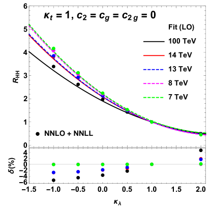
Figure 10: Comparison between $R_{\rm HH}$ obtained from Eq. 4 (line) and the ones obtained with NNLO+NNLL accuracy (points)  [18].

We observe therefore a maximal impact of the order of 5% from missing orders in QCD on $R_{\rm HH}$ calculated at LO. Still, it is hard to use this observation to derive a precise numerical recommendation on the (modest) uncertainty to be used for each point of the parameter space. Indeed the $K$-factor was obtained in the infinite top mass approximation that is challenged for large values of $m_{\rm HH}$. Moreover a non-negligible variation was observed within the BSM parameter space. In any case, since the missing order uncertainties (including $m_{t}$ effects) on $\sigma_{\rm HH,NNLO+NNLL}^{\rm SM}$ appear to be significantly larger than the ones on $R_{\rm HH}$, we recommend to neglect the latter ones with respect to the former as a leading approximation.

In summary, if one uses Eq. 4 to calculate $\sigma_{\rm HH}$ we recommend to use the uncertainties from $\sigma_{\rm HH,NNLO+NNLL}^{\rm SM}$ given in Ref. [12] and assign no specific uncertainty to $R_{\rm HH}$. Indeed, the uncertainties seem to be approximated well by the ones in the SM cross section prediction.

4.4 Translation to the Higgs basis

Obtaining the results of the fit in the H basis used by the LHCHXSWG2 [27] is straightforward. In Table 6 we provide the translation rules for the coefficients of the operators we consider from our basis to the convention of the H basis. In the latter, the coefficients of SM-like operators (the Higgs boson trilinear coupling and the top Yukawa interaction) are parameterized as additive deviations from the SM values. The pure BSM parameters in Eq. 1 are directly proportional to the corresponding coefficients in the H basis.

Operator	Coefficient
($-\cal{L}_{\rm H}$)	our basis	H basis
$\rm H^{3}$	$\kappa_{\lambda}$	$1+\delta\lambda_{3}/\lambda_{\rm SM}$
$\frac{m_{t}}{v}\rm H\,(\bar{t_{L}}t_{R}+h.c.)$	$\kappa_{t}$	$1+\delta y_{t}$
$\frac{m_{t}}{v^{2}}\rm H\rm H(\bar{t_{L}}t_{R}+h.c.)$	$c_{2}$	$y_{t}^{(2)}/2$
$-\frac{1}{4}\frac{\alpha_{s}}{3\pi v}\rm H\,G^{\mu\nu}G_{\mu\nu}$	$c_{g}$	$c_{g}^{\rm H}\,12\pi^{2}$
$-\frac{1}{4}\frac{\alpha_{s}}{3\pi v^{2}}\rm H\rm HG^{\mu\nu}G_{\mu\nu}$	$c_{2g}$	$-c_{gg}^{\rm H}\,12\pi^{2}$

Table 6: Translation of coefficients of operators (in terms of the physical fields) from our basis to the $\rm H$ basis (neglecting $CP$ violating effects).

The cross section ratio written in terms of the parameters in the H basis reads:

$$\begin{split}R_{hh}=&1+\delta\lambda_{3}(A_{1}^{\rm H}+\delta\lambda_{3}\,A_{2}^{\rm H})+\delta y_{t}\,(A_{3}^{\rm H}+\delta y_{t}\,A_{4}\,)+\delta\lambda_{3}\,\delta y_{t}\,A_{5}^{\rm H}\\[5.69054pt] &+y_{t}^{(2)}\,(A_{6}^{\rm H}+y_{t}^{(2)}\,A_{7}^{\rm H})+\delta\lambda_{3}\,y_{t}^{(2)}\,A_{8}^{\rm H}+\delta y_{t}\,y_{t}^{(2)}\,A_{9}^{\rm H}+c_{g}^{\rm H}\,(A_{10}^{\rm H}+c_{g}^{\rm H}\,A_{11})\\[5.69054pt] &+c_{gg}^{\rm H}\,(A_{12}^{\rm H}+c_{gg}^{\rm H}\,A_{13}^{\rm H})+c_{g}^{\rm H}c_{gg}^{\rm H}\,A_{14}^{\rm H}+\delta\lambda_{3}\,(c_{g}^{\rm H}\,A_{15}^{\rm H}+c_{gg}^{\rm H}\,A_{16}^{\rm H})\\[5.69054pt] &+\delta y_{t}\,(c_{g}^{\rm H}\,A_{17}^{\rm H}+c_{gg}^{\rm H}\,A_{18}^{\rm H})+y_{t}^{(2)}(c_{g}^{\rm H}\,A_{19}^{\rm H}+c_{gg}^{\rm H}\,A_{20}^{\rm H})\,.\end{split}$$ (9)

Although expanding the cross section up to quadratic order in the couplings leads to 20 coefficients $A_{i}^{\rm H}$, clearly the number of free coefficients in the fit remains the same as before. In fact, $\delta\lambda_{3},\delta y_{t}$ always enter in the combination $(1-\delta\,\cdot)^{n}$ in the matrix elements, relating different powers of the couplings. Connected to this, it is more convenient (and stable) to perform the fit actually in the parametrization of multiplicative deviations (Eq. (3)), avoiding spurious coefficients.

The central values of the coefficients of Eq. 9 are calculated using Table 6 and shown in Table 7. The rescaling of the H-gluon contact interactions makes the corresponding coefficients typically much larger than the others.

$\sqrt{s}$	7 TeV	8 TeV	13 TeV	14 TeV	100 TeV
$A_{1}^{H}$	-6.74	-6.61	-6.22	-6.17	-5.32
$A_{2}^{H}$	19.69	18.92	16.70	16.44	12.32
$A_{3}^{H}$	4.88	4.86	4.81	4.80	4.69
$A_{4}^{H}$	8.96	8.90	8.71	8.68	8.28
$A_{5}^{H}$	-25.36	-24.76	-23.00	-22.78	-19.17
$A_{6}^{H}$	-2.84	-2.84	-2.84	-2.85	-2.9
$A_{7}^{H}$	2.46	2.47	2.54	2.55	2.89
$A_{8}^{H}$	11.90	11.63	10.87	10.77	9.34
$A_{9}^{H}$	-7.22	-7.19	-7.10	-7.09	-7.02
$A_{10}^{H}$	-47.95	-46.43	-41.90	-41.32	-31.62
$A_{11}^{H}$	1693.65	1621.64	1419.59	1396.29	1037.28
$A_{12}^{H}$	-138.90	-134.89	-121.47	-119.61	-76.31
$A_{13}^{H}$	15922.80	16379.50	18682.60	19154.90	46060.00
$A_{14}^{H}$	8673.36	8475.37	7969.47	7916.62	7493.90
$A_{15}^{H}$	-17.38	-20.98	-29.47	-30.16	-35.19
$A_{16}^{H}$	867.74	840.34	761.88	752.54	600.26
$A_{17}^{H}$	-141.60	-136.56	-121.87	-120.05	-90.28
$A_{18}^{H}$	-390.60	-379.02	-341.98	-337.06	-230.66
$A_{19}^{H}$	97.58	94.69	86.32	85.34	216.14
$A_{20}^{H}$	304.87	301.54	291.21	289.94	97.71

Table 7: Central values for the coefficients entering $R_{hh}$ (Eq. (9)), employing the Higgs basis.

5 Conclusions

In this document we have shown how the wide and high-dimensional space of anomalous couplings that parametrize possible extensions of the standard model can be investigated in a systematic way, employing the example of Higgs-pair production.

We study the properties of 12 clusters, represented by benchmark points that describe the varying kinematic properties of the full multi-dimensional phase-space, and we suggest a method to study how the upper limits on the cross section of a benchmark model derived by an experimental search can be extrapolated to the points of parameter space included in the corresponding cluster.

An analytical parametrization of the cross section valid for any point of the phase space is presented and shown to deliver a good approximation of the NNLO+NNLL prediction. Precise uncertainties related to QCD parameters and missing oder effects are also offered. Using this information, an experimental analysis can easily perform an exhaustive scan of anomalous di-Higgs production within the framework of the EFT.

6 Postscript

A recent result appeard after the end of this work [14] indicates that the full top mass effects at NLO may have an impact dependent on $m_{\rm HH}$ larger than the one predicted by the approximative calculations. The calculation performed in Ref. [14] is assuing the SM case. Since no more generic calculations are yet availables for the BSM space under consideration, we let this interesting point for the further explorations of the clustering approach.

References

- [1] Martino Dall’Osso, Tommaso Dorigo, Carlo A. Gottardo, Alexandra Oliveira, Mia Tosi and Florian Goertz “Higgs Pair Production: Choosing Benchmarks With Cluster Analysis”, 2015 arXiv:1507.02245 [hep-ph]
- [2] Gerhard Buchalla “Nonlinear EFT”, 2016 URL: https://cds.cern.ch/record/2137956
- [3] W. Buchmuller and D. Wyler “Effective Lagrangian Analysis of New Interactions and Flavor Conservation” In Nucl. Phys. B268, 1986, pp. 621–653 DOI: 10.1016/0550-3213(86)90262-2
- [4] Georges Aad “Measurements of the Higgs boson production and decay rates and constraints on its couplings from a combined ATLAS and CMS analysis of the LHC collision data at 7 and 8 TeV”, 2016 arXiv:1606.02266 [hep-ex]
- [5] J. Alwall, R. Frederix, S. Frixione, V. Hirschi, F. Maltoni, O. Mattelaer, H. S. Shao, T. Stelzer, P. Torrielli and M. Zaro “The automated computation of tree-level and next-to-leading order differential cross sections, and their matching to parton shower simulations” In JHEP 07, 2014, pp. 079 DOI: 10.1007/JHEP07(2014)079
- [6] Benoit Hespel, David Lopez-Val and Eleni Vryonidou “Higgs pair production via gluon fusion in the Two-Higgs-Doublet Model” In JHEP 09, 2014, pp. 124 DOI: 10.1007/JHEP09(2014)124
- [7] Richard D. Ball “Parton distributions with LHC data” In Nucl. Phys. B867, 2013, pp. 244–289 DOI: 10.1016/j.nuclphysb.2012.10.003
- [8] Georges Aad “Search For Higgs Boson Pair Production in the Final State using Collision Data at TeV from the ATLAS Detector” In Phys. Rev. Lett. 114.8, 2015, pp. 081802 DOI: 10.1103/PhysRevLett.114.081802
- [9] Georges Aad “Searches for Higgs boson pair production in the channels with the ATLAS detector” In Phys. Rev. D 92, 2015, pp. 092004 DOI: 10.1103/PhysRevD.92.092004
- [10] Georges Aad “Search for Higgs boson pair production in the final state from pp collisions at TeV with the ATLAS detector” In Eur. Phys. J. C 75, 2015, pp. 412 DOI: 10.1140/epjc/s10052-015-3628-x
- [11] Vardan Khachatryan “Search for two Higgs bosons in final states containing two photons and two bottom quarks” Submitted to Phys. Rev. D, 2016 arXiv:1603.06896 [hep-ex]
- [12] Bruce Mellado Garcia, Pasquale Musella, Massimiliano Grazzini and Robert Harlander “CERN Report 4: Part I Standard Model Predictions”, 2016 URL: http://cds.cern.ch/record/2150771
- [13] S. Dawson, S. Dittmaier and M. Spira “Neutral Higgs boson pair production at hadron colliders: QCD corrections” In Phys. Rev. D58, 1998, pp. 115012 DOI: 10.1103/PhysRevD.58.115012
- [14] S. Borowka, N. Greiner, G. Heinrich, S. P. Jones, M. Kerner, J. Schlenk, U. Schubert and T. Zirke “Higgs boson pair production in gluon fusion at NLO with full top-quark mass dependence”, 2016 arXiv:1604.06447 [hep-ph]
- [15] Liu-Sheng Ling, Ren-You Zhang, Wen-Gan Ma, Lei Guo, Wei-Hua Li and Xiao-Zhou Li “NNLO QCD corrections to Higgs pair production via vector boson fusion at hadron colliders” In Phys. Rev. D89.7, 2014, pp. 073001 DOI: 10.1103/PhysRevD.89.073001
- [16] Jonathan Grigo, Kirill Melnikov and Matthias Steinhauser “Virtual corrections to Higgs boson pair production in the large top quark mass limit” In Nucl. Phys. B888, 2014, pp. 17–29 DOI: 10.1016/j.nuclphysb.2014.09.003
- [17] Jonathan Grigo, Jens Hoff and Matthias Steinhauser “Higgs boson pair production: top quark mass effects at NLO and NNLO” In Nucl. Phys. B900, 2015, pp. 412–430 DOI: 10.1016/j.nuclphysb.2015.09.012
- [18] Daniel Florian and Javier Mazzitelli “Higgs pair production at next-to-next-to-leading logarithmic accuracy at the LHC” In JHEP 09, 2015, pp. 053 DOI: 10.1007/JHEP09(2015)053
- [19] Daniel Florian and Javier Mazzitelli “Higgs Boson Pair Production at Next-to-Next-to-Leading Order in QCD” In Phys. Rev. Lett. 111, 2013, pp. 201801 DOI: 10.1103/PhysRevLett.111.201801
- [20] Stefano Carrazza, José I. Latorre, Juan Rojo and Graeme Watt “A compression algorithm for the combination of PDF sets” In Eur. Phys. J. C 75, 2015, pp. 474 DOI: 10.1140/epjc/s10052-015-3703-3
- [21] Jon Butterworth “PDF4LHC recommendations for LHC Run II”, 2015 arXiv:1510.03865 [hep-ph]
- [22] Sayipjamal Dulat, Tie Jiun Hou, Jun Gao, Marco Guzzi, Joey Huston, Pavel Nadolsky, Jon Pumplin, Carl Schmidt, Daniel Stump and C. P. Yuan “The CT14 Global Analysis of Quantum Chromodynamics”, 2015 arXiv:1506.07443 [hep-ph]
- [23] L. A. Harland-Lang, A. D. Martin, P. Motylinski and R. S. Thorne “Parton distributions in the LHC era: MMHT 2014 PDFs” In Eur. Phys. J. C 75, 2015, pp. 204 DOI: 10.1140/epjc/s10052-015-3397-6
- [24] Richard D. Ball “Parton distributions for the LHC Run II” In JHEP 04, 2015, pp. 040 DOI: 10.1007/JHEP04(2015)040
- [25] Christoph Peter Englert, Maxime Gouzevitch, Roberto Salerno, Magdalena Slawinska and Sara Dawson “HH: Status and recommendations for LHC HXSWG ”, 2015 URL: https://cds.cern.ch/record/2003263
- [26] Ramona Grober, Margarete Muhlleitner, Michael Spira and Juraj Streicher “NLO QCD Corrections to Higgs Pair Production including Dimension-6 Operators” In JHEP 09, 2015, pp. 092 DOI: 10.1007/JHEP09(2015)092
- [27] Michael Duehrssen-Debling, Andre Tinoco Mendes, Adam Falkowski and Gino Isidori “Higgs Basis: Proposal for an EFT basis choice for LHC HXSWG”, 2015 URL: https://cds.cern.ch/record/2001958