Globally hyperbolic moment model of arbitrary order for one-dimensional special relativistic Boltzmann equation

Abstract

This paper extends the model reduction method by the operator projection to the one-dimensional special relativistic Boltzmann equation. The derivation of arbitrary order globally hyperbolic moment system is built on our careful study of two families of the complicate ’Grad type orthogonal polynomials depending on a parameter. We derive their recurrence relations, calculate their derivatives with respect to the independent variable and parameter respectively, and study their zeros and coefficient matrices in the recurrence formulas. Some properties of the moment system are also proved. They include the eigenvalues and their bound as well as eigenvectors, hyperbolicity, characteristic fields, linear stability, and Lorentz covariance. A semi-implicit numerical scheme is presented to solve a Cauchy problem of our hyperbolic moment system in order to verify the convergence behavior of the moment method. The results show that the solutions of our hyperbolic moment system converge to the solution of the special relativistic Boltzmann equation as the order of the hyperbolic moment system increases.

1 Introduction

The beginning of the relativistic kinetic theory goes back to 1911 when an equilibrium distribution function was derived for a relativistic gas Juttner1911 . Thirty years later, the covariant formulation of the relativistic Boltzmann equation was proposed in LM1940 to describe the statistical behavior of a thermodynamic system not in thermodynamic equilibrium. The transport coefficients were determined from the Boltzmann equation by using the Chapman-Enskog methodology in Israel1963 . Different from a non-relativistic monatomic gas, a relativistic gas has a bulk viscosity. It has called the attention of many researchers to a number of applications of this theory: the effect of neutrino viscosity on the evolution of the universe, the study of galaxy formation, neutron stars, and controlled thermonuclear fusion, etc. The readers are referred to the monographs RB:2002 ; RK:1980 for more detailed descriptions.

The relativistic kinetic theory is attracting increasing attention in recent years, but it has been used relatively sparsely to model phenomenological matter in comparison to fluid models. In the non-relativistic case, the kinetic theory has been studied intensively as a mathematical subject during several decades, and also played an important role from an engineering point of view, see e.g. RB:1988 ; Cha:1970 . From the Boltzmann equation one could determine the distribution function hence the transport coefficients of gases, however this task was not so easy. Hilbert showed that an approximate solution of the integro-differential equation could be obtained from a power series expansion of a parameter (being proportional to the mean free path). Chapman and Enskog calculated independently the transport coefficients for gases whose molecules interacted according to any kind of spherically symmetric potential function. Another method proposed by Grad GRAD:1949 ; GRAD2:1949 is to expand the distribution function in terms of tensorial Hermite polynomials and introduce the balance equations corresponding to higher order moments of the distribution function. The crucial ingredient of the Chapman-Enskog method is the assumption that in the hydrodynamic regime the distribution function can be expressed as a function of the hydrodynamic variables and their gradients. The Chapman-Enskog method has been extended to the relativistic cases, see e.g. CHA2:2008 ; CHA:2012 ; CHA:2008 ; NHH:1983 ; NHH:1985 . Unfortunately, it is difficult to derive the equations of relativistic fluid dynamics from the kinetic theory DM:2012 . The moment method can avoid such difficulty and is also generalized to the relativistic cases, see e.g. Ander:1970 ; IS:1976 ; IS:1979 ; IS2:1979 ; Kranys:1972 ; Stewart:1977 . However, the moment method cannot reflect the influence of the Knudsen number. Combining the Chapman-Enskog method with the moment method has been attempted DM:2012 ; RDH:2013 .

It is difficult to derive the relativistic moment system of higher order since the family of orthogonal polynomials can not be found easily. Several authors have tried to construct the family of orthogonal polynomials analogous to the Hermite polynomials, see e.g GRADP:1974 ; RK:1980 . Their application can be found in DM:2012 ; RDH:2013 ; PRO:1998 . Unfortunately, there is no explicit expression of the moment systems if the order of the moment system is larger than $3$. Moreover, the hyperbolicity of existing general moment systems is not proved, even for the second order moment system (e.g. the general Israel and Stewart system). For a special case with heat conduction and no viscosity, Hiscock and Lindblom proved that the Israel and Stewart moment system in the Landau frame was globally hyperbolic and linearly stable, but they also showed that the Israel and Stewart moment system in the Eckart frame was not globally hyperbolic and linearly stable. The readers are referred to NHH:1987 ; NHH:1988 ; NNH:1989 . Following the approach used in NHH:1987 ; NHH:1988 , it is easy to show that the above conclusion is not true if the viscosity exists, that is, the Israel and Stewart moment system in the Landau frame is not globally hyperbolic too if the viscosity exists. There does not exist any result on the hyperbolicity or loss of hyperbolicity of (existing) general higher-order moment systems for the relativistic kinetic equation. Such proof is very difficult and challenging. The loss of hyperbolicity will cause the solution blow-up when the distribution is far away from the equilibrium state. Even for the non-relativistic case, increasing the number of moments could not avoid such blow-up FAR:2012 .

Up to now, there has been some latest progress on the Grad moment method in the non-relativistic case. A regularization was presented in 1DB:2013 for the 1D Grad moment system to achieve global hyperbolicity. It was based on the observation that the characteristic polynomial of the Jacobian of the flux in Grad’s moment system is independent of the intermediate moments, and further extended to the multi-dimensional case HY:2014 ; HG:2014 . The quadrature based projection methods were used to derive hyperbolic PDE systems for the solution of the Boltzmann equation QI:2014 ; HG2:2014 by using some quadrature rule instead of the exact integration. In the 1D case, it is similar to the regularization in 1DB:2013 . Those contributions led to well understanding the hyperbolicity of the Grad moment systems. Based on the operator projection, a general framework of model reduction technique was recently presented in MR:2014 . It projected the time and space derivatives in the kinetic equation into a finite-dimensional weighted polynomial space synchronously, and might give most of the existing moment systems mentioned above. The aim of this paper is to extend the model reduction method by the operator projection MR:2014 to the one-dimensional special relativistic Boltzmann equation and derive corresponding globally hyperbolic moment system of arbitrary order. The key is to choose the weight function and define the polynomial spaces and their basis as well as the projection operator. The theoretical foundations of our moment method are the properties of two families of the complicate Grad type orthogonal polynomials depending on a parameter.

The paper is organized as follows. Section 2 introduces the special relativistic Boltzmann equation and some macroscopic quantities defined via the kinetic theory. Section 3 gives two families of orthogonal polynomials dependent on a parameter, and studies their properties: recurrence relations, derivative relations with respect to the variable and the parameter, zeros, and the eigenvalues and eigenvectors of the recurrence matrices. Section 4 derives the moment system of the special relativistic Boltzmann equation and Section 5 studies its properties: the eigenvalues and its bound as well as eigenvectors, hyperbolicity, characteristic fields, linear stability, and Lorentz covariance. Section 6 presents a semi-implicit numerical scheme and conducts a numerical experiment to check the convergence of the proposed hyperbolic moment system. Section 7 concludes the paper. To make the main message of the paper less dilute, all proofs of theorems, lemmas and corollaries in Sections 2-6 are given in the Appendices A-E respectively.

2 Preliminaries and notations

In the special relativistic kinetic theory of gases RB:2002 , a microscopic gas particle of rest mass $m$ is characterized by the $(D+1)$ space-time coordinates $(x^{\alpha})=(x^{0},\vec{x})$ and momentum $(D+1)$-vectors $(p^{\alpha})=(p^{0},\vec{p})$, where $x^{0}=ct$, $c$ denotes the speed of light in vacuum, and $t$ and $\vec{x}$ are the time and $D$-dimensional spatial coordinates, respectively. Besides the contravariant notation (e.g. $p^{\alpha}$), the covariant notation such as $p_{\alpha}$ will be also used in the following and the covariant $p_{\alpha}$ is related to the contravariant $p^{\alpha}$ by

$$p_{\alpha}=g_{\alpha\beta}p^{\beta},\quad p^{\alpha}=g^{\alpha\beta}p_{\beta},$$

where $(g^{\alpha\beta})$ denotes the Minkowski space-time metric tensor and is chosen as
$(g^{\alpha\beta})={\rm diag}\{1,-\vec{I}_{D}\}$, $\vec{I}_{D}$ is the $D\times D$ identity matrix, $(g_{\alpha\beta})$ denotes the inverse of $(g^{\alpha\beta})$, and the Einstein summation convention over repeated indices is used. For a free relativistic particle, one has the relativistic energy-momentum relation (aka “on-shell” or “mass-shell” condition) $E^{2}-\vec{p}^{2}c^{2}=m^{2}c^{4}$. If putting $p^{0}=c^{-1}E=\sqrt{\vec{p}^{2}+m^{2}c^{2}}$, then the “mass-shell” condition can be rewritten as $p^{\alpha}p_{\alpha}=m^{2}c^{2}$.

As in the non-relativistic case, the relativistic Boltzmann equation describes the evolution of the one-particle distribution function of an ideal gas in the phase space spanned by the space-time coordinates $(x^{\alpha})$ and momentum (D+1)-vectors of particles $(p^{\alpha})$. The one-particle distribution function depends only on $(\vec{x},\vec{p},t)$ and is defined in such a way that $f(\vec{x},\vec{p},t)d^{D}\vec{x}d^{D}\vec{p}$ gives the number of particles at time $t$ in the volume element $d^{D}\vec{x}d^{D}\vec{p}$. For a single gas the Boltzmann equation reads RB:2002

$$p^{\alpha}\frac{\partial f}{\partial x^{\alpha}}=Q(f,f),$$ (2.1)

where the collision term $Q(f,f)$ depends on the product of the distribution functions of two particles at collision, e.g.

$$Q(f,f)=\int_{\mathbb{R}^{{D}}}\int_{\mathbb{S}^{{D-1}}_{+}}\left(f_{*}^{\prime}f^{\prime}-f_{*}f\right)Bd{\Omega}\frac{d^{{D}}\vec{p}_{*}}{p_{*}^{0}},$$

where $f$ and $f_{*}$ are the distributions depending on the momenta before a collision, while $f^{\prime}$ and $f_{*}^{\prime}$ depend on the momenta after the collision, $d\Omega$ denotes the element of the solid angle, the collision kernel $B=\sigma\sqrt{(p_{*}^{\alpha}p_{\alpha})^{2}-m^{2}c^{2}}$ for a single non degenerate gas (e.g. electron gas), and $\sigma$ denotes the differential cross section of collision,. The collision term satisfies

$$\int_{\mathbb{R}^{{D}}}Q(f,f)\frac{d^{D}\vec{p}}{p^{0}}=0,\quad\int_{\mathbb{R}^{{D}}}p^{\alpha}Q(f,f)\frac{d^{D}\vec{p}}{p^{0}}=0,$$ (2.2)

so that $1$ and $p^{\alpha}$ are called collision invariants. Moreover, the Boltzmann equation (2.1) should satisfy the entropy dissipation relation (in the sense of classical statistics)

$$\int_{\mathbb{R}^{D}}Q(f,f)\ln(f)\frac{d^{D}\vec{p}}{p^{0}}\leq 0,$$

where the equal sign corresponds to the local thermodynamic equilibrium.

In kinetic theory the macroscopic description of gas can be represented by the first and second moments of the distribution function $f$, namely, the partial particle (D+1)-flow $N^{\alpha}$ and the partial energy-momentum tensor $T^{\alpha\beta}$, which are defined by

$$N^{\alpha}=c\int_{{\mathbb{R}^{D}}}p^{\alpha}f\frac{d^{D}\vec{p}}{p^{0}},\quad T^{\alpha\beta}=c\int_{{\mathbb{R}^{D}}}p^{\alpha}p^{\beta}f\frac{d^{D}\vec{p}}{p^{0}}.$$ (2.3)

They can be decomposed into the following forms (i.e. the Landau-Lifshitz decomposition)

$$N^{\alpha} ={m^{-1}}\rho U^{\alpha}+n^{\alpha},$$ (2.4)

$$T^{\alpha\beta} =c^{-2}\varepsilon U^{\alpha}U^{\beta}-\Delta^{\alpha\beta}(P_{0}+\Pi)+\pi^{\alpha\beta},$$ (2.5)

where $(U^{\alpha})=\left(\gamma(\vec{u})c,\gamma(\vec{u})\vec{u}\right)$ denotes the macroscopic velocity $(D+1)$-vector of gases, $\gamma(\vec{u})=(1-c^{-2}|\vec{u}|^{2})^{-\frac{1}{2}}$ is the Lorentz factor, $\Delta^{\alpha\beta}$ is defined by

$$\Delta^{\alpha\beta}:=g^{\alpha\beta}-c^{-2}U^{\alpha}U^{\beta},$$ (2.6)

which is symmetric and the projector onto the $D$-dimensional subspace orthogonal to $U^{\alpha}$, that is, satisfies $\Delta^{\alpha\beta}U_{\beta}=0$. Here, the mass density $\rho$, the particle-diffusion current $n^{\alpha}$, the energy density $\varepsilon$, the shear-stress tensor $\pi^{\alpha\beta}$, and the sum of thermodynamic pressure $P_{0}$ and bulk viscous pressure $\Pi$ are defined and related to the distribution $f$ by

$$\rho:=c^{-2}{m}U_{\alpha}N^{\alpha}=c^{-1}{m}\int_{\mathbb{R}^{D}}Ef\frac{d^{D}\vec{p}}{p^{0}},$$ (2.7)

$$n^{\alpha}:=\Delta^{\alpha}_{\beta}N^{\beta}=c\int_{\mathbb{R}^{D}}p^{<\alpha>}f\frac{d^{D}\vec{p}}{p^{0}},$$

$$\varepsilon:=c^{-2}U_{\alpha}U_{\beta}T^{\alpha\beta}=c^{-1}\int_{\mathbb{R}^{D}}E^{2}f\frac{d^{D}\vec{p}}{p^{0}},$$

$$\pi^{\alpha\beta}:=\Delta_{\mu\nu}^{\alpha\beta}T^{\mu\nu}=c\int_{\mathbb{R}^{D}}p^{<\alpha\beta>}f\frac{d^{D}\vec{p}}{p^{0}},$$

$$P_{0}+\Pi:=-D^{-1}\Delta_{\alpha\beta}T^{\alpha\beta}=D^{-1}c^{-1}\int_{\mathbb{R}^{D}}(E^{2}-{m^{2}}c^{4})f\frac{d^{D}\vec{p}}{p^{0}},$$

where $E:=U_{\alpha}p^{\alpha}$ here and hereafter, $p^{<\alpha>}:=\Delta_{\beta}^{\alpha}p^{\beta}$, $p^{<\alpha\beta>}:=\Delta^{\alpha\beta}_{\mu\nu}{p^{\mu}p^{\nu}}$, and

$$\Delta^{\alpha\beta}_{\mu\nu}:=\frac{1}{2}\left(\Delta_{\mu}^{\alpha}\Delta_{\nu}^{\beta}+\Delta_{\mu}^{\beta}\Delta_{\nu}^{\alpha}-2D^{-1}\Delta_{\mu\nu}\Delta^{\alpha\beta}\right).$$

It is obvious to obtain

$$U_{\alpha}p^{<\alpha>}=0.$$ (2.8)

It is not difficult to verify the following identity

$$p^{\alpha}=c^{-2}EU^{\alpha}+p^{<\alpha>}.$$ (2.9)

Multiplying the special relativistic Boltzmann equation (2.1) by $1$ and $p^{\alpha}$ respectively, integrating both sides over $\mathbb{R}^{D}$ in terms of $\vec{p}$, and using (2.2) gives the following conservation laws

$$\partial_{\alpha}N^{\alpha}=0,\quad\partial_{\alpha}T^{\alpha\beta}=0.$$ (2.10)

Remark 1

It is common to choose $U^{\alpha}$ as the velocity of either energy transport (the Landau-Lifshitz frame) Lau:1949 ), i.e.

$$U_{\beta}T^{\alpha\beta}=\varepsilon U^{\alpha},$$ (2.11)

i.e.

$$\Delta^{\alpha}_{\beta}T^{\beta\gamma}U_{\gamma}=c\int_{{\mathbb{R}^{D}}}Ep^{<\alpha>}f\frac{d^{D}\vec{p}}{p^{0}}=0,$$ (2.12)

or particle transport (the Eckart frame) EC:1940 ), i.e. in which the velocity is specified by the flow of particles

$$N^{\alpha}={m^{-1}}\rho U^{\alpha},$$

i.e.

$$\Delta^{\alpha}_{\beta}{N^{\beta}}=c\int_{{\mathbb{R}^{D}}}\Delta^{\alpha}_{\beta}{p^{\beta}}f\frac{d^{D}\vec{p}}{p^{0}}=0.$$

The former can be applied to multicomponent gas while the latter is only used for single component gas. This work will be done in the Landau-Lifshitz frame (2.11).

Remark 2

At the local thermodynamic equilibrium, $n^{\alpha}$, $\Pi$, and $\pi^{\alpha\beta}$ will be zero.

Remark 3

In order to simplify the collision term, several simple collision models have been proposed, see RB:2002 . Similar to the BGK (Bhatnagar-Gross-Krook) model in the non-relativistic theory, two simple relativistic collision models are the Marle model MM:1965

$$Q(f,f)=-\frac{m}{\tau}(f-f^{(0)}),$$ (2.13)

and the Anderson-Witting model AW:1974

$$Q(f,f)=-\frac{U_{\alpha}p^{\alpha}}{\tau{c^{2}}}(f-f^{(0)}),$$ (2.14)

where $f^{(0)}=f^{(0)}(\vec{x},\vec{p},t)$ denotes the distribution function at the local thermodynamic equilibrium, and $\tau$ is the relaxation time and may rely on $\rho$, $\theta$. In the non-relativistic limit, both models (2.13) and (2.14) tend to the BGK model. However, the Marle model (2.13) does not satisfy the constraints of the collision terms in (2.2). The relaxation time $\tau$ can be defined by

$$\tau=\frac{1}{n\pi d^{2}\bar{g}},$$

where $n$ denotes the particle number density, $d$ denotes the diameter of gas particles, and $\bar{g}$ is proportional to the mean relative speed $\bar{\xi}$ between two particles, e.g. $\bar{g}=\sqrt{2}\bar{\xi}$ or $\bar{\xi}$ RB:2002 . In the non-relativistic case, $\bar{\xi}=4\sqrt{\frac{kT}{\pi m}}$, but the expression of $\bar{\xi}$ in relativistic case is very complicate, see Section 8.2 of book RB:2002 . Usually, $\bar{\xi}$ or $\bar{g}$ is suitably approximated, for example, $\bar{g}\approx c$ (that is, $\bar{g}$ is approximated by using the ultra-relativistic limit). Under such simple approximation, one has

$$\tau\approx\frac{1}{n\pi d^{2}c}=\frac{m}{\rho\pi d^{2}c}.$$

This paper will only consider the one-dimensional form of relativistic Boltzmann equation (2.1). In this case, the vector notations $\vec{x}$ and $\vec{p}$ will be replaced with $x$ or $x^{1}$ and $p$ or $p^{1}$, respectively, the Greek indices $\alpha$ and $\beta$ run from 0 to 1, and (2.1) reduces to the following form

$$p^{0}\frac{\partial f}{\partial ct}+p^{1}\frac{\partial f}{\partial x}=Q(f,f),\quad t\in\mathbb{R}^{+},\ x\in\mathbb{R}.$$ (2.15)

In the $1$D case, the shear-stress tensor $\pi^{\alpha\beta}$ disappears even though the local-equilibrium is departed from, and the local-equilibrium distribution $f^{(0)}$ can be explicitly given by

$$f^{(0)}=\rho g^{(0)},\quad g^{(0)}=\frac{1}{2{m^{2}}cK_{1}(\zeta)}\exp\left(-\zeta E\right),$$ (2.16)

which is like the Maxwell-Jüttner distribution RB:2002 for the case of $D=3$ and Maxwell gas

$${f^{(0)}=\rho g^{(0)},\quad g^{(0)}=\frac{\zeta}{4\pi m^{4}c^{3}K_{2}(\zeta)}\exp\left(-\zeta E\right),}$$

and obeys the common prescription that the mass density $\rho$ and energy density $\varepsilon$ are completely determined by the local-equilibrium distribution $f^{(0)}$ alone, that is,

$$\rho=\rho_{0},\quad\varepsilon=\varepsilon_{0}.$$ (2.17)

In (2.16), $\zeta={(k_{B}T)^{-1}(mc^{2})}$ is the ratio between the particle rest energy $mc^{2}$ and the thermal energy of the gas $k_{B}T$, $k_{B}$ denotes the Boltzmann constant, $T$ is the thermodynamic temperature, and $K_{n}(\zeta)$ denotes the modified Bessel function of the second kind, defined by

$$K_{n}(\zeta)=\int_{0}^{\infty}\cosh(n\vartheta)\exp(-\zeta\cosh\vartheta)d\vartheta,$$ (2.18)

satisfying the recurrence relation

$$K_{n+1}(\zeta)=K_{n-1}(\zeta)+2n\zeta^{-1}K_{n}(\zeta).$$ (2.19)

For $\zeta\gg 1$ the particles behave as non-relativistic, and for $\zeta\ll 1$ they behave as ultra-relativistic.

Similar to (2.7), from the knowledge of the equilibrium distribution function $f^{(0)}$ it is also possible to determine the values of some macroscopic variables by

$$\rho_{0}:=c^{-1}{m}\int_{\mathbb{R}}Ef^{(0)}\frac{dp}{p^{0}},$$ (2.20)

$$n^{\alpha}_{0}:=c\int_{\mathbb{R}}p^{<\alpha>}f^{(0)}\frac{dp}{p^{0}}=0,$$

$$\varepsilon_{0}:=c^{-1}\int_{\mathbb{R}}E^{2}f^{(0)}\frac{dp}{p^{0}}={\rho}c^{2}\left(G(\zeta)-\zeta^{-1}\right),$$

$$P_{0}:=c^{-1}\int_{\mathbb{R}}(E^{2}-{m^{2}}c^{4})f^{(0)}\frac{dp}{p^{0}}={m^{-1}}\rho k_{B}T={\rho c^{2}\zeta^{-1}},$$

where $G(\zeta):=K_{1}^{-1}(\zeta)K_{2}(\zeta)$. Now, the conservation laws (2.10) become

$$\frac{\partial\left(\rho U^{0}\right)}{\partial ct}+\frac{\partial\left(\rho U^{1}\right)}{\partial x}=0,$$ (2.21)

$$\frac{\partial\left(c^{-2}\rho hU^{0}U^{1}\right)}{\partial ct}+\frac{\partial\left(c^{-2}\rho hU^{1}U^{1}+P_{0}\right)}{\partial x}=0,$$

$$\frac{\partial\left(c^{-2}\rho hU^{0}U^{0}-P_{0}\right)}{\partial ct}+\frac{\partial\left(c^{-2}\rho hU^{0}U^{1}\right)}{\partial x}=0,$$

where $h:=\rho^{-1}(\varepsilon+P_{0})={c^{2}}G(\zeta)$ denotes the specific enthalpy. They are just the macroscopic equations of special relativistic hydrodynamics (RHD). In other words, when $f=f^{(0)}$, the special relativistic Boltzmann equation (2.15) can lead to the RHD equations (2.21). We aim at finding reduced model equations to describe states with $f\neq f^{(0)}$. This paper will extend the moment method by operator projection MR:2014 to (2.15) and derive its arbitrary order moment model in Section 4.

Before ending this section, we discuss the macroscopic variables calculated by a given distribution $f$, in other words, for the nonnegative distribution $f(x,p,t)$, which is not identically zero, can the physically admissible macroscopic states $\{\rho,u,\theta={\zeta}^{-1}\}$ satisfying $\rho>0,|u|<{c}$ and $\theta>0$ be obtained?

Theorem 2.1

For the nonnegative distribution $f(x,p,t)$, which is not identically zero, the density current $N^{\alpha}$ and energy-momentum tensor $T^{\alpha\beta}$ calculated by (2.3) satisfy

$$(T^{00}+T^{11})^{2}>4(T^{01})^{2},\quad N^{0}-{c^{-1}u}N^{1}>0,\quad{c^{-2}\rho^{-1}(T^{00}-c^{-1}uT^{01})}>1,$$ (2.22)

where the macroscopic velocity $u$ is the unique solution satisfying $|u|<{c}$ of the quadratic equation

$${T^{01}c^{-2}u^{2}-(T^{00}+T^{11})c^{-1}u+T^{01}=0},$$ (2.23)

which has a solution satisfying ${|u|<c}$ and

$$u=\left\{\begin{array}[]{ll}\frac{T^{00}+T^{11}-\sqrt{(T^{00}+T^{11})^{2}-4(T^{01})^{2}}}{2T^{01}c^{-1}},&\hbox{$T^{01}\neq 0$,}\\ 0,&\hbox{$T^{01}=0$.}\end{array}\right.$$ (2.24)

And the positive mass density $\rho$ is calculated by

$$\rho={c^{-1}m\frac{N^{0}-c^{-1}uN^{1}}{\sqrt{1-c^{-2}u^{2}}}}.$$ (2.25)

Furthermore, the equation

$${G(\theta^{-1})-\theta=c^{-2}\rho^{-1}(T^{00}-c^{-1}uT^{01})},$$ (2.26)

has a unique positive solution $\theta$ in the interval $(0,+\infty)$.

Furthermore, the following conclusion holds.

Theorem 2.2

Under the assumptions of Theorem 2.1, the bulk viscous pressure $\Pi$ satisfies

$$\Pi>-\rho{c^{2}}\theta.$$

Remark 4

The proofs of those theorems are given in the Appendix A. Theorem 2.1 provides a recovery procedure of the admissible primitive variables $\rho,u$, and $\theta$ from the nonnegative distribution $f(x,p,t)$ or the given density current $N^{\alpha}$ and energy-momentum tensor $T^{\alpha\beta}$ satisfying (2.22). It is useful in the derivation of the moment system as well as the numerical scheme.

Before discussing the moment method, we first non-dimensionalize the relativistic Boltzmann equation (2.15). Here we only consider the Anderson-Witting model (2.14). If setting

$$x=L\hat{x},~{}p=c\hat{p},~{}p^{0}=c\hat{p^{0}},~{}t=\frac{L}{c}\hat{t},~{}g=c\hat{g},~{}f=\frac{n_{0}}{c^{3}}\hat{f},$$

where $L$ denotes the macroscopic characteristic length, $n_{0}$ and $\theta_{0}=mc^{2}/k_{B}$ are the reference particle number and temperature, respectively, then the 1D relativistic Boltzmann equation (2.15) with (2.14) is non-dimensionalized as follows

$$\frac{n_{0}}{c^{2}L}\left(p^{0}\frac{\partial\hat{f}}{\partial\hat{t}}+p^{1}\frac{\partial\hat{f}}{\partial\hat{x}}\right)=\frac{n_{0}^{2}\pi d^{2}}{c^{2}}\hat{U}_{\alpha}\hat{p}^{\alpha}\hat{\rho}\left(\hat{f}^{(0)}-\hat{f}\right),$$

or

$$\hat{p}^{0}\frac{\partial\hat{f}}{\partial\hat{t}}+\hat{p}^{1}\frac{\partial\hat{f}}{\partial\hat{x}}=n_{0}L\pi d^{2}\hat{U}_{\alpha}\hat{p}^{\alpha}\hat{\rho}\left(\hat{f}^{(0)}-\hat{f}\right).$$

Thanks to $K_{n}=\frac{\lambda}{L}=\frac{\tau_{0}c}{L}=\frac{1}{n_{0}L\pi d^{2}}$, the above equation is rewritten as

$$\hat{p}^{0}\frac{\partial\hat{f}}{\partial\hat{t}}+\hat{p}^{1}\frac{\partial\hat{f}}{\partial\hat{x}}=\frac{\hat{\rho}}{K_{n}}\hat{U}_{\alpha}\hat{p}^{\alpha}\left(\hat{f}^{(0)}-\hat{f}\right).$$ (2.27)

Thus, if $\tilde{\tau}:=\frac{K_{n}}{\hat{\rho}}$ may be considered as a new “relaxation time”, then the collision term of relativistic Boltzmann equation (2.27) has the same form of non-relativistic BGK model. For the sake of convenience, in the following, we still use $\tau$, $x$, $t$, $f$, $p$, $p^{0}$, $\rho$ to replace $\tilde{\tau}$, $\hat{x}$, $\hat{t}$, $\hat{f}$, $\hat{p}$, $\hat{p}^{0}$, $\hat{\rho}$, respectively.

3 Two families of orthogonal polynomials

This section introduces two families of orthogonal polynomials dependent on a parameter $\zeta$, similar to those given in GRADP:1974 , and studies their properties, which will be used in the derivation and discussion of our moment system. All proofs are given in the Appendix B.

If considering

$$\omega^{(\ell)}(x;\zeta)=\frac{(x^{2}-1)^{\ell-\frac{1}{2}}}{K_{1}(\zeta)}\exp(-\zeta x),\ \ell=0,1,$$

as the weight functions in the interval $[1,+\infty)$, where $\zeta\in\mathbb{R}^{+}$ denotes a parameter, then the inner products with respect to $\omega^{(\ell)}(x;\zeta)$ can be introduced as follows

$$\left(f,g\right)_{\omega^{(\ell)}}:=\int_{1}^{+\infty}f(x)g(x)\omega^{(\ell)}(x;\zeta)dx,\quad f,g\in L^{2}_{\omega^{(\ell)}}[1,+\infty),\ \ell=0,1,$$

where $L^{2}_{\omega^{(\ell)}}[1,+\infty):=\left\{f\big{|}\int_{1}^{+\infty}f(x)^{2}\omega^{(\ell)}(x;\zeta)dx<+\infty\right\}$. It is worth noting that the choice of the weight function $\omega^{(\ell)}(x;\zeta)$ is dependent on the equilibrium distribution $f^{(0)}(x,p,t)$ in (2.16).

Let $\{P_{n}^{(\ell)}(x;\zeta)\}$, $\ell=0,1$, be two families of standard orthogonal polynomials with respect to the weight function $\omega^{(\ell)}(x;\zeta)$ in the interval $[1,+\infty)$, i.e.

$$\left(P_{m}^{(\ell)},P_{n}^{(\ell)}\right)_{\omega^{(\ell)}}=\delta_{m,n},\quad\ell=0,1,$$ (3.1)

where $\delta_{m,n}$ denotes the Kronecker delta function, which is equal to 1 if $m=n$, and 0 otherwise. Obviously, $\{P_{n}^{(\ell)}(x;\zeta)\}$ satisfies

$$\left(P_{n}^{(\ell)},x^{k}\right)_{\omega^{(\ell)}}=0,\ k\leq n-1,$$ (3.2)

which imply

$$Q(x;\zeta)=\sum_{i=0}^{n}\left(x^{n},P_{n}^{(\ell)}\right)_{\omega^{(\ell)}}P_{n}^{(\ell)}(x;\zeta),$$ (3.3)

for any polynomial $Q(x;\zeta)$ of degree $\leq n$ in $L^{2}_{\omega^{(\ell)}}[1,+\infty)$.

The orthogonal polynomials $\{P_{n}^{(\ell)}(x;\zeta)\}$ can be obtained by using the Gram-Schmidt process. For example, several orthogonal polynomials of lower degree are given as follows

$$\begin{aligned} P_{0}^{(0)}(x;\zeta)&=\frac{1}{\sqrt{G(\zeta)-2\zeta^{-1}}},\\ P_{1}^{(0)}(x;\zeta)&=\frac{\sqrt{G(\zeta)-2\zeta^{-1}}}{\sqrt{G(\zeta)^{2}-3\zeta^{-1}G(\zeta)+2\zeta^{-2}-1}}\left(x-\frac{1}{G(\zeta)-2\zeta^{-1}}\right),\\ P_{2}^{(0)}(x;\zeta)&=\frac{\zeta\sqrt{G(\zeta)^{2}-3\zeta^{-1}G(\zeta)+2\zeta^{-2}-1}}{\sqrt{2G(\zeta)^{3}-7\zeta^{-1}G(\zeta)^{2}-2G(\zeta)+6\zeta^{-2}G(\zeta)+\zeta^{-1}}}\\ &\cdot\left(x^{2}-\frac{G(\zeta)^{2}-2\zeta^{-1}G(\zeta)-1}{\zeta\left(G(\zeta)^{2}-3\zeta^{-1}G(\zeta)+2\zeta^{-2}-1\right)}x-\frac{G(\zeta)^{2}-3\zeta^{-1}G(\zeta)+\zeta^{-2}-1}{G(\zeta)^{2}-3\zeta^{-1}G(\zeta)+2\zeta^{-2}-1}\right),\\ P_{0}^{(1)}(x;\zeta)&=\sqrt{\zeta},\\ P_{1}^{(1)}(x;\zeta)&=\frac{\sqrt{\zeta}}{\sqrt{-G(\zeta)^{2}+3\zeta^{-1}G(\zeta)+1}}\left(x-G(\zeta)\right),\end{aligned}$$ (3.4)

plotted in Fig. 3.1 with respect to $x$ and $\zeta$.

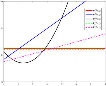
(a) $x-P_{n}^{(\ell)}(x,\zeta)$ with $\zeta=1$.

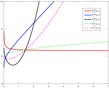
(b) $\zeta-P_{n}^{(\ell)}(x,\zeta)$ with $x=3$.

Figure 3.1: Values of the polynomials in (3.4) with respect to $x$ in (a) and $\zeta$ in (b).

It shows that the coefficients in those orthogonal polynomials are so irregular that it will be very complicate to study the properties of $\{P_{n}^{(\ell)}(x;\zeta)\}$. Let $c_{n}^{(\ell)}$ be the leading coefficient of $P_{n}^{(\ell)}(x;\zeta)$, $\ell=0,1$. Without loss of generality, assume $c_{n}^{(\ell)}>0$, $\ell=0,1$. Due to the important result on the zeros of orthogonal polynomials (SP:2011, , Theorem 3.2), the polynomial $P_{n}^{(\ell)}(x;\zeta)$ has exactly $n$ real simple zeros in the interval $(1,+\infty)$, $\ell=0,1$. Thus if those zeros are denoted by $\{x_{i,n}^{(\ell)}\}_{i=1}^{n}$ in an increasing order, then the polynomial $P_{n}^{(\ell)}(x;\zeta)$ can be rewritten as follows

$$P_{n}^{(\ell)}(x;\zeta)=c_{n}^{(\ell)}\prod_{i=1}^{n}(x-x_{i,n}^{(\ell)}).$$ (3.5)

In the following, we want to derive the recurrence relations of $\{P_{n}^{(\ell)}(x;\zeta)\}$, calculate their derivatives with respect to $x$ and $\zeta$, respectively, and study the properties of zeros and coefficient matrices in the recurrence relations.

3.1 Recurrence relations

This section presents the recurrence relations for the orthogonal polynomials $\{P_{n}^{(\ell)}(x;\zeta)\}$, $\ell=0,1$, the recurrence relations between $\{P_{n}^{(0)}(x;\zeta)\}$ and $\{P_{n}^{(1)}(x;\zeta)\}$, and the specific forms of the coefficients in those recurrence relations.

Using the three-term recurrence relation and the existence theorem of zeros of general orthogonal polynomials in Theorems 3.1 and 3.2 of SP:2011 gives the following conclusion.

Theorem 3.1

For $\ell=0,1$, a three-term recurrence relation for the orthogonal polynomials $\{P_{n}^{(\ell)}(x;\zeta)\}$ can be given by

$$xP_{n}^{(\ell)}=a_{n-1}^{(\ell)}P_{n-1}^{(\ell)}+b_{n}^{(\ell)}P_{n}^{(\ell)}+a_{n}^{(\ell)}P_{n+1}^{(\ell)},$$ (3.6)

or in the matrix-vector form

$$x\vec{P}_{n}^{(\ell)}=\vec{J}_{n}^{(\ell)}\vec{P}_{n}^{(\ell)}+a_{n}^{(\ell)}P_{n+1}^{(\ell)}\vec{e}_{n+1},\ \vec{P}_{n}^{(\ell)}:=(P_{0}^{(\ell)},\cdots,P_{n}^{(\ell)})^{T},$$ (3.7)

where both coefficients

$$a_{n}^{(\ell)}:=\left(xP_{n}^{(\ell)},P_{n+1}^{(\ell)}\right)_{\omega^{(\ell)}}=\frac{c_{n}^{(\ell)}}{c_{n+1}^{(\ell)}},\quad b_{n}^{(\ell)}:=\left(xP_{n}^{(\ell)},P_{n}^{(\ell)}\right)_{\omega^{(\ell)}}=\sum_{i=1}^{n+1}x_{i,n+1}^{(\ell)}-\sum_{i=1}^{n}x_{i,n}^{(\ell)},$$ (3.8)

are positive, $\vec{e}_{n+1}$ is the last column of the identity matrix of order $(n+1)$, and

$$\vec{J}_{n}^{(\ell)}:=\begin{pmatrix}b_{0}^{(\ell)}&a_{0}^{(\ell)}&0&&&\\ a_{0}^{(\ell)}&b_{1}^{(\ell)}&a_{1}^{(\ell)}&&&\\ &\ddots&\ddots&\ddots&&\\ &&&a_{n-2}^{(\ell)}&b_{n-1}^{(\ell)}&a_{n-1}^{(\ell)}\\ &&&0&a_{n-1}^{(\ell)}&b_{n}^{(\ell)}\\ \end{pmatrix}\in{\mathbb{R}}^{(n+1)\times(n+1)},$$

which is symmetric positive definite tridiagonal matrix with the spectral radius larger than $1$.

Besides, the recurrence relations between $\{P_{n}^{(0)}(x;\zeta)\}$ and $\{P_{n}^{(1)}(x;\zeta)\}$ can also be obtained.

Theorem 3.2

(i) Two three-term recurrence relations between $\{P_{n}^{(0)}(x;\zeta)\}$ and $\{P_{n}^{(1)}(x;\zeta)\}$ can be given by

$$(x^{2}-1)P_{n}^{(1)}=p_{n}P_{n}^{(0)}+q_{n}P_{n+1}^{(0)}+r_{n+1}P_{n+2}^{(0)},$$ (3.9)

$$P_{n+1}^{(0)}=r_{n}P_{n-1}^{(1)}+q_{n}P_{n}^{(1)}+p_{n+1}P_{n+1}^{(1)},$$ (3.10)

or in the matrix-vector form

$$\vec{P}_{n+1}^{(0)} =\vec{J}_{n}^{T}\vec{P}_{n}^{(1)}+p_{n+1}P_{n+1}^{(1)}\vec{e}_{n+2},$$ (3.11)

$$(x^{2}-1)\vec{P}_{n}^{(1)} =\vec{J}_{n}\vec{P}_{n+1}^{(0)}+r_{n+1}P_{n+2}^{(0)}\vec{e}_{n+1},$$ (3.12)

where

$$p_{n}:=\frac{c_{n}^{(0)}}{c_{n}^{(1)}},q_{n}:=\frac{c_{n}^{(1)}}{c_{n+1}^{(0)}}\left(\sum_{i=1}^{n+2}x_{i,n+2}^{(0)}-\sum_{i=1}^{n}x_{i,n}^{(1)}\right)=\frac{c_{n+1}^{(0)}}{c_{n}^{(1)}}\sum_{i=1}^{n+1}(x_{i,n+1}^{(1)}-x_{i,n+1}^{(0)}),r_{n}:=\frac{c_{n-1}^{(1)}}{c_{n+1}^{(0)}},$$ (3.13)

and

$$\vec{J}_{n}:=\begin{pmatrix}p_{0}&q_{0}&r_{1}&0&0&\cdots&0\\ 0&p_{1}&q_{1}&r_{2}&0&\cdots&0\\ \ &\ddots&\ddots&\ddots&\ &\ &\ \\ \ &\ &\ &\ &0&p_{n}&q_{n}\end{pmatrix}\in{\mathbb{R}}^{(n+1)\times(n+2)}.$$

(ii) Two two-term recurrence relations between $\{P_{n}^{(0)}(x;\zeta)\}$ and $\{P_{n}^{(1)}(x;\zeta)\}$ can be derived as follows

$$(x^{2}-1)P_{n}^{(1)}=\tilde{p}_{n}(x+\tilde{q}_{n})P_{n+1}^{(0)}+\tilde{r}_{n}P_{n}^{(0)},$$ (3.14)

$$P_{n+1}^{(0)}=\frac{1}{\tilde{p}_{n}}(x-\tilde{q}_{n})P_{n}^{(1)}-\frac{a_{n-1}^{(1)}}{a_{n}^{(0)}}\tilde{r}_{n}P_{n-1}^{(1)},$$ (3.15)

where

$$\tilde{p}_{n}:=\frac{c_{n}^{(1)}}{c_{n+1}^{(0)}},\quad\tilde{q}_{n}:=\sum_{i=1}^{n+1}x_{i,n+1}^{(0)}-\sum_{i=1}^{n}x_{i,n}^{(1)},\quad\tilde{r}_{n}:={p_{n}(1-\tilde{p}_{n}^{2})}.$$ (3.16)

3.2 Partial derivatives

This section calculates the derivatives of the polynomial $P_{n}^{(\ell)}(x;\zeta)$ with respect to $x$ and $\zeta$, $\ell=0,1$.

Theorem 3.3

For $\ell=0,1$, the first-order derivative of the polynomial $P_{n+1}^{(\ell)}(x;\zeta)$ with respect to the parameter $\zeta$ satisfies

$$\frac{\partial P_{n+1}^{(\ell)}}{\partial\zeta}=a_{n}^{(\ell)}P_{n}^{(\ell)}-\frac{1}{2}\left(G(\zeta)-\zeta^{-1}-b_{n+1}^{(\ell)}\right)P_{n+1}^{(\ell)}.$$ (3.17)

Theorem 3.4

The first-order derivatives of the polynomials $\{P_{n}^{(\ell)}(x;\zeta)\}$ with respect to the variable $x$ satisfy

$$\frac{\partial P_{n+1}^{(0)}}{\partial x}=\frac{n+1}{\tilde{p}_{n}}P_{n}^{(1)}+\zeta r_{n}P_{n-1}^{(1)},$$ (3.18)

$$(x^{2}-1)\frac{\partial P_{n}^{(1)}}{\partial x}+xP_{n}^{(1)}=(n+1)\tilde{p}_{n}P_{n+1}^{(0)}+\zeta p_{n}P_{n}^{(0)}.$$ (3.19)

3.3 Zeros

Using the separation theorem of zeros of general orthogonal polynomials SP:2011 gives the following conclusion on our orthogonal polynomials $\{P_{n}^{(\ell)}(x;\zeta)\}$.

Theorem 3.5

For $\ell=0,1$, the zeros $\{x_{i,n}^{(\ell)}\}_{i=1}^{n}$ of $P_{n}^{(\ell)}(x;\zeta)$ and $\{x_{i,n+1}^{(\ell)}\}_{i=1}^{n+1}$ of $P_{n+1}^{(\ell)}(x;\zeta)$ satisfy the separation property

$$1<x_{1,n+1}^{(\ell)}<x_{1,n}^{(\ell)}<x_{2,n+1}^{(\ell)}<\cdots<x_{n,n}^{(\ell)}<x_{n+1,n+1}^{(\ell)}.$$

There is still another important separation property for the zeros of the orthogonal polynomials $\{P_{n}^{(\ell)}(x;\zeta),\ell=0,1\}$.

Theorem 3.6

The $n$ zeros $\{x_{i,n}^{(1)}\}_{i=1}^{n}$ of $P_{n}^{(1)}$ and $n+1$ zeros of $\{x_{i,n+1}^{(0)}\}_{i=1}^{n+1}$ of $P_{n+1}^{(0)}$ satisfy

$$1<x_{1,n+1}^{(0)}<x_{1,n}^{(1)}<x_{2,n+1}^{(0)}<\cdots<x_{n,n}^{(1)}<x_{n+1,n+1}^{(0)}.$$

According to Theorems 3.5 and 3.6, we can further know the sign of the coefficients of the recurrence relations in Theorem 3.2.

Corollary 1

All quantities $p_{n},q_{n},r_{n}$ in (3.13) and $\tilde{p}_{n},\tilde{q}_{n},\tilde{r}_{n}$ in (3.16) are positive.

Using Corollary 1, $\tilde{r}_{n}={p_{n}(1-\tilde{p}_{n}^{2})}$, and $\tilde{p}_{n}=(c_{n+1}^{(0)})^{-1}c_{n}^{(1)}$ give the following corollary.

Corollary 2

The leading coefficient of $P_{n+1}^{(0)}$ is larger than that of $P_{n}^{(1)}$, i.e. $c_{n+1}^{(0)}>c_{n}^{(1)}$.

According to Theorems 3.3 and 3.5, we have further the following conclusion.

Corollary 3

The zeros $\{x_{i,n}^{(\ell)}\}_{i=1}^{n}$ of $P_{n}^{(\ell)}$ strictly decrease with respect to $\zeta$, i.e.

$$\frac{\partial x_{i,n}^{(\ell)}}{\partial\zeta}<0.$$

3.4 Generalized eigenvalues and eigenvectors of coefficient matrices in the recurrence relations

This section discusses the generalized eigenvalues and eigenvectors of two $(2n+1)\times(2n+1)$ matrices $\vec{A}^{0}_{n}$ and $\vec{A}^{1}_{n}$, defined by

$$\vec{A}^{0}_{n}:=\begin{pmatrix}\vec{J}_{n}^{(0)}&\vec{O}\\ \vec{O}&\vec{J}_{n-1}^{(1)}\end{pmatrix},\quad\vec{A}^{1}_{n}:=\begin{pmatrix}\vec{O}&\vec{J}_{n-1}^{T}\\ \vec{J}_{n-1}&\vec{O}\end{pmatrix},$$ (3.20)

where $\vec{J}_{n}^{(0)}$, $\vec{J}_{n}^{(1)}$, and $\vec{J}_{n}$ appear in the recurrence relations in Theorems 3.1 and 3.2.

Consider the following generalized eigenvalue problem (2nd sense): Find a vector $\vec{y}$ that obeys $\vec{A}^{1}_{n}\vec{y}=\hat{\lambda}\vec{A}^{0}_{n}\vec{y}$. If let $\vec{u}$ denote the first $n+1$ rows of $\vec{y}$, and $\vec{v}$ be the last $n$ rows of $\vec{y}$, then

$$\hat{\lambda}\vec{J}_{n}^{(0)}\vec{u}=\vec{J}_{n-1}^{T}\vec{v},\quad\hat{\lambda}\vec{J}_{n-1}^{(1)}\vec{v}=\vec{J}_{n-1}\vec{u}.$$ (3.21)

Multiplying (3.7), (3.11), and (3.12) by $P_{n}^{(1)}(-x;\zeta)$ with $|x|>1$ gives

$$\vec{P}_{n}^{(0)}(x;\zeta)P_{n}^{(1)}(-x;\zeta)=\frac{1}{x}\vec{J}_{n}^{(0)}\vec{P}_{n}^{(0)}(x;\zeta)P_{n}^{(1)}(-x;\zeta)+\frac{1}{x}a_{n}^{(0)}P_{n+1}^{(0)}(x;\zeta)P_{n}^{(1)}(-x;\zeta)\vec{e}_{n+1},$$ (3.22)

$$\vec{P}_{n-1}^{(1)}(x;\zeta)P_{n}^{(1)}(-x;\zeta)=\frac{1}{x}\vec{J}_{n-1}^{(1)}\vec{P}_{n-1}^{(1)}(x;\zeta)P_{n}^{(1)}(-x;\zeta)+\frac{1}{x}a_{n-1}^{(1)}P_{n}^{(1)}(x;\zeta)P_{n}^{(1)}(-x;\zeta)\vec{e}_{n},$$ (3.23)

$$\vec{P}_{n}^{(0)}(x;\zeta)P_{n}^{(1)}(-x;\zeta)=\vec{J}_{n-1}^{T}\vec{P}_{n-1}^{(1)}(x;\zeta)P_{n}^{(1)}(-x;\zeta)+p_{n}P_{n}^{(1)}(x;\zeta)P_{n}^{(1)}(-x;\zeta)\vec{e}_{n+1},$$ (3.24)

$$(x^{2}-1)\vec{P}_{n-1}^{(1)}(x;\zeta)P_{n}^{(1)}(-x;\zeta)=\vec{J}_{n-1}\vec{P}_{n}^{(0)}(x;\zeta)P_{n}^{(1)}(-x;\zeta)+r_{n}P_{n+1}^{(0)}(x;\zeta)P_{n}^{(1)}(-x;\zeta)\vec{e}_{n}.$$ (3.25)

If substituting (3.22) and (3.23) into (3.24) and(3.25) respectively, then one obtains

$$\vec{J}_{n}^{(0)} \vec{P}_{n}^{(0)}(x;\zeta)P_{n}^{(1)}(-x;\zeta)=x\vec{J}_{n-1}^{T}\vec{P}_{n-1}^{(1)}(x;\zeta)P_{n}^{(1)}(-x;\zeta)$$

$$+\left(xp_{n}P_{n}^{(1)}(x;\zeta)P_{n}^{(1)}(-x;\zeta)-a_{n}^{(0)}P_{n+1}^{(0)}(x;\zeta)P_{n}^{(1)}(-x;\zeta)\right)\vec{e}_{n+1},$$ (3.26)

$$\frac{x^{2}-1}{x} \vec{J}_{n-1}^{(1)}\vec{P}_{n-1}^{(1)}(x;\zeta)P_{n}^{(1)}(-x;\zeta)=\vec{J}_{n-1}\vec{P}_{n}^{(0)}(x;\zeta)P_{n}^{(1)}(-x;\zeta)$$

$$+\left(r_{n}P_{n+1}^{(0)}(x;\zeta)P_{n}^{(1)}(-x;\zeta)-\frac{x^{2}-1}{x}a_{n-1}^{(1)}P_{n}^{(1)}(x;\zeta)P_{n}^{(1)}(-x;\zeta)\right)\vec{e}_{n}.$$ (3.27)

Transforming (3.26) and (3.27) by $x$ to $-x$ and then adding them into (3.26) and (3.27) respectively gives

$$\frac{\sqrt{x^{2}-1}}{x}\vec{J}_{n}^{(0)}\vec{u}(x;\zeta)=\vec{J}_{n-1}^{T}\vec{v}(x;\zeta)-\frac{\sqrt{x^{2}-1}}{x}a_{n}^{(0)}Q_{2n}(x;\zeta)\vec{e}_{n+1},$$ (3.28)

$$\frac{\sqrt{x^{2}-1}}{x}\vec{J}_{n-1}^{(1)}\vec{v}(x;\zeta)=\vec{J}_{n-1}\vec{u}(x;\zeta)+r_{n}Q_{2n}(x;\zeta)\vec{e}_{n},$$ (3.29)

for $|x|>1$, where

$$\vec{u}(x;\zeta)= \vec{P}_{n}^{(0)}(x;\zeta)P_{n}^{(1)}(-x;\zeta)+\vec{P}_{n}^{(0)}(-x;\zeta)P_{n}^{(1)}(x;\zeta),$$

$$\vec{v}(x;\zeta)= \sqrt{x^{2}-1}\left(\vec{P}_{n-1}^{(1)}(x;\zeta)P_{n}^{(1)}(-x;\zeta)-\vec{P}_{n-1}^{(1)}(-x;\zeta)P_{n}^{(1)}(x;\zeta)\right),$$

and

$$Q_{2n}(x;\zeta):=P_{n+1}^{(0)}(x;\zeta)P_{n}^{(1)}(-x;\zeta)+P_{n+1}^{(0)}(-x;\zeta)P_{n}^{(1)}(x;\zeta).$$ (3.30)

It is not difficult to find that if the second terms at the right-hand sides of (3.28) and (3.29) disappear, then (3.28) and (3.29) reduce to two equations in (3.21). Thus in order to obtain the generalized eigenvalues and eigenvectors of $\vec{A}_{n}^{0}$ and $\vec{A}_{n}^{1}$, one has to study the zeros of $Q_{2n}(x;\zeta)$.

Lemma 1

The function $Q_{2n}(x;\zeta)$ is an even polynomial of degree $2n$ and has $2n$ real simple zeros $\{z_{i,n},i=\pm 1,\cdots,\pm n\}$, which satisfy $z_{-i,n}=-z_{i,n}$ and $z_{i,n}\in(1,+\infty)$ for $i=1,\cdots,n$.

The polynomials $Q_{10}(x;\zeta)$, $P^{(0)}_{5}(x;\zeta)$, $P^{(0)}_{6}(x;\zeta)$, $P^{(1)}_{4}(x;\zeta)$, and $P^{(1)}_{5}(x;\zeta)$ with $\zeta=1$ are plotted in Fig. 3.2, where the relation between their zeros can be clearly observed.

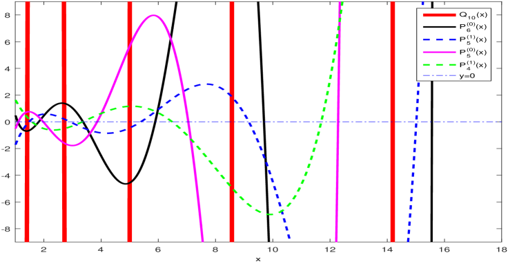
Figure 3.2: Plots of the polynomials $Q_{10}(x;\zeta)$, $P^{(0)}_{5}(x;\zeta)$, $P^{(0)}_{6}(x;\zeta)$, $P^{(1)}_{4}(x;\zeta)$, and $P^{(1)}_{5}(x;\zeta)$ with $\zeta=1$.

With the aid of Theorems 3.3 and 3.4, we can calculate the partial derivatives at $z_{i,n}$ of $Q_{2n}(x;\zeta)$ with respect to $x$ and $\zeta$.

Lemma 2

At the positive zeros $\{z_{i,n}\}_{i=1}^{n}$, the partial derivatives of $Q_{2n}(x;\zeta)$ satisfy

$$\frac{\partial Q_{2n}}{\partial\zeta}(z_{i,n};\zeta)= 2\frac{P_{n}^{(1)}(z_{i,n};\zeta)}{P_{n}^{(1)}(-z_{i,n};\zeta)}\frac{a_{n}^{(0)}}{\tilde{r}_{n}}\left((\tilde{p}_{n}+\tilde{p}_{n}^{-1})z_{i,n}P_{n}^{(1)}(-z_{i,n};\zeta)P_{n+1}^{(0)}(-z_{i,n};\zeta)\right.$$

$$\left.+(z_{i,n}^{2}-1)P_{n}^{(1)}(-z_{i,n};\zeta)^{2}+P_{n+1}^{(0)}(-z_{i,n};\zeta)^{2}\right),$$

$$\frac{\partial Q_{2n}}{\partial x}(z_{i,n};\zeta)= 2\zeta\frac{P_{n}^{(1)}(z_{i,n};\zeta)}{P_{n}^{(1)}(-z_{i,n};\zeta)}\frac{a_{n}^{(0)}}{\tilde{r}_{n}}\left((\tilde{p}_{n}+\tilde{p}_{n}^{-1})P_{n+1}^{(0)}(-z_{i,n};\zeta)P_{n}^{(1)}(-z_{i,n};\zeta)\right.$$

$$\left.+z_{i,n}P_{n}^{(1)}(-z_{i,n};\zeta)^{2}+z_{i,n}(z_{i,n}^{2}-1)^{-1}P_{n+1}^{(0)}(-z_{i,n};\zeta)^{2}\right).$$

Moreover, one has

$${\rm sign}\left(\frac{\partial Q_{2n}}{\partial\zeta}(z_{i,n};\zeta)\right)={\rm sign}\left(\frac{\partial Q_{2n}}{\partial x}(z_{i,n};\zeta)\right)={\rm sign}\left(\frac{P_{n}^{(1)}(z_{i,n};\zeta)}{P_{n}^{(1)}(-z_{i,n};\zeta)}\right).$$ (3.31)

Similar to Corollary 3, the following conclusion holds.

Lemma 3

The zeros $\{z_{i,n},i=\pm 1,\cdots,\pm{n}\}$ of $Q_{2n}(x;\zeta)$ satisfy

$$\frac{\partial z_{i,n}}{\partial\zeta}<0,\ i=1,\cdots,n;\quad\frac{\partial z_{i,n}}{\partial\zeta}>0,\ i=-n,\cdots,-1.$$

Thanks to Lemmas 1 and 3, the generalized eigenvalues and eigenvectors of two
$(2n+1)\times(2n+1)$ matrices $\vec{A}^{0}_{n}$ and $\vec{A}^{1}_{n}$ can be obtained with the aid of the zeros of $Q_{2n}(x;\zeta)$.

Theorem 3.7

Besides a zero eigenvalue denoted by $\hat{\lambda}_{0,n}$, the matrix pair $\vec{A}^{0}_{n}$ and $\vec{A}^{1}_{n}$ has $2n$ non-zero, real and simple generalized eigenvalues, which satisfy

$$\hat{\lambda}_{i,n}:=\frac{\sqrt{z_{i,n}^{2}-1}}{z_{i,n}},\quad|\hat{\lambda}_{i,n}|<1,\ i=\pm 1,\cdots,\pm n,$$ (3.32)

and

$$\frac{\partial\hat{\lambda}_{i,n}}{\partial\zeta}<0,\ i=1,\cdots,n;\quad\frac{\partial\hat{\lambda}_{i,n}}{\partial\zeta}>0,\ i=-n,\cdots,-1.$$ (3.33)

Corresponding $(2n+1)$ generalized eigenvectors can be expressed as

$$\vec{y}_{i,n}:=\left(\vec{u}_{i,n}^{T},\vec{v}_{i,n}^{T}\right)^{T},$$ (3.34)

with

$$\begin{aligned} &\vec{u}_{i,n}=\vec{P}_{n}^{(0)}(z_{i,n};\zeta)P_{n}^{(1)}(-z_{i,n});\zeta+\vec{P}_{n}^{(0)}(-z_{i,n};\zeta)P_{n}^{(1)}(z_{i,n};\zeta),\\ &\vec{v}_{i,n}=\sqrt{z_{i,n}^{2}-1}\left(\vec{P}_{n-1}^{(1)}(z_{i,n};\zeta)P_{n}^{(1)}(-z_{i,n};\zeta)-\vec{P}_{n-1}^{(1)}(-z_{i,n};\zeta)P_{n}^{(1)}(z_{i,n};\zeta)\right).\end{aligned}$$ (3.35)

for $i=\pm 1,\cdots,\pm n$, and

$$\vec{u}_{0,n}=\vec{P}_{n}^{(0)}(1;\zeta)P_{n+1}^{(0)}(-1;\zeta)-\vec{P}_{n}^{(0)}(-1;\zeta)P_{n+1}^{(0)}(1;\zeta),\quad\vec{v}_{0,n}={0}.$$ (3.36)

4 Moment method by operator projection

This section begins to extend the moment method by operator projection MR:2014 to the one-dimensional relativistic Boltzmann equation (2.15) and derive its arbitrary order hyperbolic moment model. For the sake of convenience, without loss of generality, units in which both the speed of light $c$ and rest mass $m$ of particle are equal to one will be used in the following. All proofs are given in the Appendix C.

4.1 Weighted polynomial space

In order to use the moment method by the operator projection to derive the hyperbolic moment model of the kinetic equation, we should define weighted polynomial spaces and norms as well as the projection operator. Thanks to the equilibrium distribution $f^{(0)}$ in (2.16), the weight function is chosen as $g^{(0)}$, which will be replaced with the new notation $g^{(0)}_{[u,\theta]}$, considering the dependence of $g^{(0)}$ on the macroscopic fluid velocity $u$ and $\theta=k_{B}T/m=\zeta^{-1}$, that is

$$g^{(0)}_{[u,\theta]}=\frac{1}{2K_{1}(\zeta)}\exp\left(-\frac{E}{\theta}\right),\ E=U_{\alpha}p^{\alpha}.$$ (4.1)

Associated with the weight function $g^{(0)}_{[u,\theta]}$, our weighted polynomial space is defined by

$$\mathbb{H}^{g^{(0)}_{[u,\theta]}}:={\rm span}\left\{p^{\mu_{1}}p^{\mu_{2}}\cdots p^{\mu_{\ell}}g^{(0)}_{[u,\theta]}:\ \ \mu_{i}=0,1,\ \ell\in\mathbb{N}\right\},$$

which is an infinite-dimensional linear space equipped with the inner product

$$<f,g>_{g^{(0)}_{[u,\theta]}}:=\int_{\mathbb{R}}\frac{1}{g^{(0)}_{[u,\theta]}}f(p)g(p)\frac{dp}{p^{0}},\quad f,g\in\mathbb{H}^{g^{(0)}_{[u,\theta]}}.$$

Similarly, for a finite positive integer $M\in\mathbb{N}$, a finite-dimensional weighted polynomial space can be defined by

$$\mathbb{H}^{g^{(0)}_{[u,\theta]}}_{M}:={\rm span}\left\{p^{\mu_{1}}p^{\mu_{2}}\cdots p^{\mu_{\ell}}g^{(0)}_{[u,\theta]}:\ \ \mu_{i}=0,1,\ \ell=0,1,\cdots,M\right\},$$

which is a closed subspace of $\mathbb{H}^{g^{(0)}_{[u,\theta]}}$ obviously.

Thanks to Theorem 2.2, for all physically admissible $u$ and $\theta$ satisfying $|u|<1$ and $\theta>0$, introduce two notations

$$\vec{\mathcal{P}}_{\infty}[u,\theta]:= (\tilde{P}_{0}^{(0)}[u,\theta],\tilde{P}_{1}^{(0)}[u,\theta],\tilde{P}_{0}^{(1)}[u,\theta],\cdots,\tilde{P}_{M}^{(0)}[u,\theta],\tilde{P}_{M-1}^{(1)}[u,\theta],\cdots)^{T},$$ (4.2)

$$\vec{\mathcal{P}}_{M}[u,\theta]:= (\tilde{P}_{0}^{(0)}[u,\theta],\tilde{P}_{1}^{(0)}[u,\theta],\tilde{P}_{0}^{(1)}[u,\theta],\cdots,\tilde{P}_{M}^{(0)}[u,\theta],\tilde{P}_{M-1}^{(1)}[u,\theta])^{T},$$ (4.3)

where $\tilde{P}_{k}^{(0)}[u,\theta]=g^{(0)}_{[u,\theta]}P_{k}^{(0)}$ and $\tilde{P}_{k}^{(1)}[u,\theta]=g^{(0)}_{[u,\theta]}(U^{0})^{-1}P_{k}^{(1)}p_{<1>}$.

Lemma 4

The set of all components of $\vec{\mathcal{P}}_{\infty}[u,\theta]$ (resp. $\vec{\mathcal{P}}_{M}[u,\theta]$) form a standard orthogonal basis of $\mathbb{H}^{g^{(0)}_{[u,\theta]}}$ (resp. $\mathbb{H}^{g^{(0)}_{[u,\theta]}}_{M}$).

Remark 5

In the non-relativistic limit, $E=U_{\alpha}p^{\alpha}$, $p_{<1>}$ and $g^{(0)}_{[u,\theta]}$ reduce to $p^{2}$, $-p$ and $\frac{1}{\sqrt{2\pi\theta}}\exp(-\frac{p^{2}}{\theta})$, respectively, thus the basis become the generalized Hermite polynomials 1DB:2013 .

Since $\mathbb{H}^{g^{(0)}_{[u,\theta]}}_{M}$ is a subspace of $\mathbb{H}^{g^{(0)}_{[u,\theta]}}_{N}$ when $M<N<+\infty$, there exists a matrix
$P_{M,N}\in\mathbb{R}^{(2M+1)\times(2N+1)}$ with full row rank such that $\vec{\mathcal{P}}_{M}[u,\theta]=P_{M,N}\vec{\mathcal{P}}_{N}[u,\theta]$, where

$$\vec{P}_{M,N}:={\rm diag}\{\vec{I}_{2M+1,2M+1},\vec{O}_{2M+1,2N-2M}\}.$$

Using the properties of the orthogonal polynomials $\{P_{n}^{(\ell)}(x;\zeta),\ell=0,1,n\geq 0\}$ in Section 3 can further give calculation of the partial derivatives and recurrence relations of the basis functions $\{\tilde{P}_{n}^{(0)}[u,\theta],n\geq 0\}$ and $\{\tilde{P}_{n-1}^{(1)}[u,\theta],n\geq 1\}$.

Lemma 5 (Derivative relations)

The partial derivatives of basis functions
$\{\tilde{P}_{n}^{(0)}[u,\theta],n\geq 0\}$ and $\{\tilde{P}_{n-1}^{(1)}[u,\theta],n\geq 1\}$ can be calculated by

$$\frac{\partial\tilde{P}_{n}^{(0)}[u,\theta]}{\partial s}= -\frac{\partial\theta}{\partial s}\zeta^{2}\left(\frac{1}{2}\left(G(\zeta)-\zeta^{-1}-b_{n}^{(0)}\right)\tilde{P}_{n}^{(0)}[u,\theta]-a_{n}^{(0)}\tilde{P}_{n+1}^{(0)}[u,\theta]\right)$$

$$+\frac{\partial u}{\partial s}\frac{1}{(1-u^{2})}\left(\left(n\tilde{p}_{n-1}^{-1}-\zeta q_{n-1}\right)\tilde{P}_{n-1}^{(1)}[u,\theta]-\zeta p_{n}\tilde{P}_{n}^{(1)}[u,\theta]\right),$$

$$\frac{\partial\tilde{P}_{n-1}^{(1)}[u,\theta]}{\partial s}= -\frac{\partial\theta}{\partial s}\zeta^{2}\left(\frac{1}{2}\left(G(\zeta)-\zeta^{-1}-b_{n-1}^{(1)}\right)\tilde{P}_{n-1}^{(1)}[u,\theta]+a_{n-1}^{(1)}\tilde{P}_{n}^{(1)}[u,\theta]\right)$$

$$+\frac{\partial u}{\partial s}\frac{1}{1-u^{2}}\left(\left(n\tilde{p}_{n-1}-\zeta q_{n-1}\right)\tilde{P}_{n}^{(0)}[u,\theta]-\zeta r_{n}\tilde{P}_{n+1}^{(0)}[u,\theta]\right),$$

for $s=t$ and $x$. It indicates that $\frac{\partial\tilde{P}_{M}^{(0)}}{\partial s}$ and $\frac{\partial\tilde{P}_{M-1}^{(0)}}{\partial s}$ $\in\mathbb{H}^{g^{(0)}_{[u,\theta]}}_{M+1}$.

Lemma 6 (Recurrence relations)

The basis functions
$\{\tilde{P}_{n}^{(0)}[u,\theta],n\geq 0\}$ and $\{\tilde{P}_{n-1}^{(1)}[u,\theta]$, $n\geq 1\}$ satisfy the following recurrence relations

$$p^{0}\vec{\mathcal{P}}_{M}[u,\theta]= \vec{M}_{M}^{t}\vec{\mathcal{P}}_{M}[u,\theta]$$ (4.4)

$$+\left(-U^{1}p_{M}\tilde{P}_{M}^{(1)}[u,\theta]+U^{0}a_{M}^{(0)}\tilde{P}_{M+1}^{(0)}[u,\theta]\right)\vec{e}_{2M+1}^{1}$$

$$+\left(-U^{1}r_{M}\tilde{P}_{M+1}^{(0)}[u,\theta]+U^{0}a_{M-1}^{(1)}\tilde{P}_{M}^{(1)}[u,\theta]\right)\vec{e}_{2M+1}^{2},$$

$$p\vec{\mathcal{P}}_{M}[u,\theta]= \vec{M}_{M}^{x}\vec{\mathcal{P}}_{M}[u,\theta]$$

$$+\left(-U^{0}p_{M}\tilde{P}_{M}^{(1)}[u,\theta]+U^{1}a_{M}^{(0)}\tilde{P}_{M+1}^{(0)}[u,\theta]\right)\vec{e}_{2M+1}^{1}$$

$$+\left(-U^{0}r_{M}\tilde{P}_{M+1}^{(0)}[u,\theta]+U^{1}a_{M-1}^{(1)}\tilde{P}_{M}^{(1)}[u,\theta]\right)\vec{e}_{2M+1}^{2},$$

where $\vec{e}_{2M+1}^{1}$ and $\vec{e}_{2M+1}^{2}$ are the penultimate and the last column of the identity matrix of order $(2M+1)$, respectively, and

$$\vec{M}_{M}^{t}: =-U^{1}\vec{P}_{M}^{p}\vec{A}_{M}^{1}(\vec{P}_{M}^{p})^{T}+U^{0}\vec{P}_{M}^{p}\vec{A}_{M}^{0}(\vec{P}_{M}^{p})^{T},$$ (4.5)

$$\vec{M}_{M}^{x}: =-U^{0}\vec{P}_{M}^{p}\vec{A}_{M}^{1}(\vec{P}_{M}^{p})^{T}+U^{1}\vec{P}_{M}^{p}\vec{A}_{M}^{0}(\vec{P}_{M}^{p})^{T},$$

in which $\vec{P}_{M}^{p}$ is a permutation matrix making

$$\vec{P}_{M}^{p}\vec{\mathcal{\tilde{P}}}_{M}[u,\theta]=\vec{\mathcal{P}}_{M}[u,\theta],\quad$$ (4.6)

with

$$\vec{\mathcal{\tilde{P}}}_{M}[u,\theta]:=(\tilde{P}_{0}^{(0)}[u,\theta],\cdots,\tilde{P}_{M}^{(0)}[u,\theta],\tilde{P}_{0}^{(1)}[u,\theta],\cdots,\tilde{P}_{M-1}^{(1)}[u,\theta])^{T}.$$

For a finite integer $M\geq 1$, define an operator $\Pi_{M}[u,\theta]:\mathbb{H}^{g^{(0)}_{[u,\theta]}}\rightarrow\mathbb{H}^{g^{(0)}_{[u,\theta]}}_{M}$ by

$$\Pi_{M}[u,\theta]f:=\sum_{i=0}^{M}f_{i}^{0}\tilde{P}_{i}^{(0)}[u,\theta]+\sum_{j=0}^{M-1}f_{j}^{1}\tilde{P}_{j}^{(1)}[u,\theta],$$ (4.7)

or in a compact form

$$\Pi_{M}[u,\theta]f=[\vec{\mathcal{P}}_{M}[u,\theta],\vec{f}_{M}]_{M},$$ (4.8)

where

$$f_{i}^{0} =<f,\tilde{P}_{i}^{(0)}[u,\theta]>_{g^{(0)}_{[u,\theta]}},\ i\leq M,\ \ f_{j}^{1}=<f,\tilde{P}_{j}^{(1)}[u,\theta]>_{g^{(0)}_{[u,\theta]}},\ j\leq M-1,$$ (4.9)

$$\vec{f}_{M} =(f_{0}^{0},f_{1}^{0},f_{0}^{1},\cdots,f_{M}^{0},f_{M-1}^{1})^{T}.$$ (4.10)

and the symbol $[\cdot,\cdot]_{M}$ denotes the common inner product of two $(2M+1)$-dimensional vectors.

Lemma 7

The operator $\Pi_{M}[u,\theta]$ is linear bounded and projection operator in sense that

(i)

$\Pi_{M}[u,\theta]f\in\mathbb{H}^{g^{(0)}_{[u,\theta]}}_{M}$ for all $f\in\mathbb{H}^{g^{(0)}_{[u,\theta]}}$,

(ii)

$\Pi_{M}[u,\theta]f=f$ for all $f\in\mathbb{H}^{g^{(0)}_{[u,\theta]}}_{M}$.

Remark 6

The so-called Grad type expansion is to expand the distribution function $f(x,p,t)$ in the weighted polynomial space $\mathbb{H}^{g^{(0)}_{[u,\theta]}}$ as follows

$$f(x,p,t)=\left[\vec{\mathcal{P}}_{\infty}[u,\theta],\vec{f}_{\infty}\right]_{\infty},$$

where the symbol $[\cdot,\cdot]_{\infty}$ denotes the common inner product of two infinite-dimensional vectors, and $\vec{f}_{\infty}=(f_{0}^{0},f_{1}^{0},f_{0}^{1},\cdots,f_{M}^{0},f_{M-1}^{1},\cdots)^{T}$.

4.2 Derivation of the moment model

Based on the weighted polynomial spaces $\mathbb{H}^{g^{(0)}_{[u,\theta]}}$ and $\mathbb{H}^{g^{(0)}_{[u,\theta]}}_{M}$ in Section 4.1 and the projection operator $\Pi_{M}[u,\theta]$ defined in (4.7), the moment method by the operator projection MR:2014 can be implemented for the 1D special relativistic Boltzmann equation (2.15). In view of the fact that the variables $\{\rho,u,\theta,\Pi,{n}^{1}\}$ are several physical quantities of practical interest and the first three are required in calculating the equilibrium distribution $f^{(0)}$.

The $(2M+1)$-dimensional vector

$$\vec{W_{M}}=(\rho,u,\theta,\Pi,\tilde{n}^{1},f_{3}^{0},f_{2}^{1},\cdots,f_{M}^{0},f_{M-1}^{1})^{T},$$

will be considered as the dependent variable vector, instead of $\vec{f}_{M}$ defined in (4.10), where $\tilde{n}^{1}:=n^{1}\sqrt{1-u^{2}}$. The relations between $\vec{W_{M}}$ and $\vec{f_{M}}$ is

$$\vec{f}_{M}=\vec{D}_{M}^{W}\vec{W}_{M},$$ (4.11)

where the square matrix $\vec{D}_{M}^{\vec{W}}$ depends on $\theta$ and is of the following explicit form

$$\vec{D}_{1}^{W}=\begin{pmatrix}(c_{0}^{(0)})^{-1}&0&0\\ 0&0&0\\ 0&0&0\end{pmatrix},\quad\vec{D}_{2}^{W}=\begin{pmatrix}(c_{0}^{(0)})^{-1}&0&0&{c_{0}^{(0)}}&0\\ 0&0&0&c_{1}^{(0)}x_{1,1}^{(0)}&0\\ 0&0&0&0&-c_{0}^{(1)}\\ 0&0&0&{-}c_{2}^{(0)}x_{1,2}^{(0)}x_{2,2}^{(0)}&0\\ 0&0&0&0&{c_{1}^{(1)}}x_{1,1}^{(1)}\end{pmatrix},$$

and $\vec{D}_{M}^{W}={\rm diag}\{\vec{D}_{2}^{W},\vec{I}_{2M-4}\}$ for $M\geq 3$, which is derived from (2.12) and (2.17).

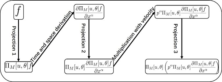
Figure 4.1: Schematic diagram of the moment method by the operator projection for the 1D special relativistic Boltzmann equation.

Referring to the schematic diagram shown in Fig. 4.1, the arbitrary order moment system for the Boltzmann equation (2.15) can be derived by the operator projection as follows:

Step 1 (Projection 1): Projecting the distribution function $f$ into space $\mathbb{H}^{g^{(0)}_{[u,\theta]}}_{M}$ by the operator $\Pi_{M}[u,\theta]$ defined in (4.8).

Step 2: Calculating the partial derivatives in time and space provides

$$\frac{\partial\Pi_{M}[u,\theta]f}{\partial s} =\left[\frac{\partial\vec{\mathcal{P}}_{M}[u,\theta]}{\partial s},\vec{f}_{M}\right]_{M}+\left[\vec{\mathcal{P}}_{M}[u,\theta],\frac{\partial\vec{f}_{M}}{\partial s}\right]_{M}$$

$$=\left[\vec{C}_{M+1}\vec{P}_{M,M+1}^{T}\vec{\mathcal{P}}_{M}[u,\theta],\vec{P}_{M,M+1}^{T}\vec{f}_{M}\right]_{M+1}+\left[\vec{\mathcal{P}}_{M}[u,\theta],\frac{\partial\vec{f}_{M}}{\partial s}\right]_{M},$$ (4.12)

for $s=t$ and $x$, where $\vec{C}_{M+1}$ is a square matrix of order $(2M+3)$ and directly derived with the aid of the derivative relations of the basis functions in Lemma 5.

Step 3 (Projection 2): Projecting the partial derivatives in (4.12) into the space $\mathbb{H}^{g^{(0)}_{[u,\theta]}}_{M}$ gives

$$\Pi_{M}[u,\theta]\frac{\partial\Pi_{M}[u,\theta]f}{\partial s} =\left[\vec{\mathcal{P}}_{M}[u,\theta],\vec{C}_{M}^{T}\vec{f}_{M}\right]_{M}+\left[\vec{\mathcal{P}}_{M}[u,\theta],\frac{\partial\vec{f}_{M}}{\partial s}\right]_{M}$$

$$=\left[\vec{\mathcal{P}}_{M}[u,\theta],\vec{C}_{M}^{T}\vec{D}_{M}^{W}\vec{W}_{M}+\frac{\partial\left(\vec{D}_{M}^{W}\vec{W}_{M}\right)}{\partial s}\right]_{M}$$

$$=:\left[\vec{\mathcal{P}}_{M}[u,\theta],\vec{D}_{M}\frac{\partial\vec{W}_{M}}{\partial s}\right]_{M},$$ (4.13)

where the $(2M+1)$-by-$(2M+1)$ matrix $\vec{D}_{M}$ can be obtained from $\vec{C}_{M}$ and $\vec{D}_{M}^{\vec{W}}$ and is of the following form

$$\vec{D}_{M}=\begin{pmatrix}&\ &\ &D_{2}&\ &\ &O&\ &\ \\ &0&*&*&0&\ &\ &\ &\ \\ &\vdots&\vdots&\vdots&\ &\ &\vec{I}_{2M-4}&\ &\\ \ &0&*&*&0&\ &\ &\ &\ \end{pmatrix},\ M\geq 3,$$ (4.14)

and

$$\vec{D}_{2} =\begin{pmatrix}(c_{0}^{(0)})^{-1}&0&-\rho\zeta^{2}(c_{1}^{(0)})^{-2}(c_{0}^{(0)})^{-1}&{c_{0}^{(0)}}&0\\ 0&(1-u^{2})^{-1}c_{1}^{(0)}\tilde{n}^{1}&\rho\zeta^{2}(c_{1}^{(0)})^{-1}&c_{1}^{(0)}x_{1,1}^{(0)}&0\\ 0&-(1-u^{2})^{-1}c_{0}^{(1)}\rho&0&0&-c_{0}^{(1)}\\ 0&-(1-u^{2})^{-1}c_{2}^{(0)}\tilde{n}^{1}(x_{1,2}^{(0)}+x_{2,2}^{(0)})&0&{-}c_{2}^{(0)}x_{1,2}^{(0)}x_{2,2}^{(0)}&0\\ 0&-(1-u^{2})^{-1}c_{1}^{(1)}\Pi&0&0&{c_{1}^{(1)}}x_{1,1}^{(1)}\end{pmatrix},$$

$$\vec{D}_{1} =\begin{pmatrix}(c_{0}^{(0)})^{-1}&0&-\rho\zeta^{2}(c_{1}^{(0)})^{-2}(c_{0}^{(0)})^{-1}\\ 0&0&\rho\zeta^{2}(c_{1}^{(0)})^{-1}\\ 0&-(1-u^{2})^{-1}c_{0}^{(1)}\rho&0\end{pmatrix},$$

where the elements “$*$” of $\vec{D}_{M}$ in (4.14) are explicitly given by

$$\vec{D}_{M}(2n+1,2) =\frac{1}{(1-u^{2})}\left(\left(n\tilde{p}_{n-1}-\zeta q_{n-1}\right)f_{n-1}^{1}-\zeta r_{n-1}f_{n-2}^{1}\right),$$

$$\vec{D}_{M}(2n+2,2) =\frac{1}{(1-u^{2})}\left(\left((n+1)\tilde{p}_{n}^{-1}-\zeta q_{n}\right)f_{n+1}^{0}-\zeta p_{n}f_{n}^{0}\right),$$

$$\vec{D}_{M}(2n+1,3) =-\zeta^{2}\left(\frac{1}{2}\left(G(\zeta)-\zeta^{-1}-b_{n}^{(0)}\right)f_{n}^{0}-a_{n-1}^{(0)}f_{n-1}^{0}\right),$$

$$\vec{D}_{M}(2n+1,3) =-\zeta^{2}\left(\frac{1}{2}\left(G(\zeta)-\zeta^{-1}-b_{n}^{(1)}\right)f_{n}^{1}+a_{n-1}^{(1)}f_{n-1}^{1}\right).$$

Step 4: Multiplying (4.13) by the particle velocity $(p^{\alpha})$ yields

$$p^{0}\Pi_{M}[u,\theta]\frac{\partial\Pi_{M}[u,\theta]f}{\partial{t}} :=[p^{0}\vec{\mathcal{P}}_{M}[u,\theta],\vec{D}_{M}\frac{\partial\vec{W}_{M}}{\partial{t}}]_{M}$$

$$=[\vec{M}_{M+1}^{t}\vec{P}_{M,M+1}^{T}\vec{\mathcal{P}}_{M}[u,\theta],\vec{P}_{M,M+1}^{T}\vec{D}_{M}\frac{\partial\vec{W}_{M}}{\partial{t}}]_{M+1},$$ (4.15)

$$p\Pi_{M}[u,\theta]\frac{\partial\Pi_{M}[u,\theta]f}{\partial{x}} :=[p\vec{\mathcal{P}}_{M}[u,\theta],\vec{D}_{M}\frac{\partial\vec{W}_{M}}{\partial{x}}]_{M}$$

$$=[\vec{M}_{M+1}^{x}\vec{P}_{M,M+1}^{T}\vec{\mathcal{P}}_{M}[u,\theta],\vec{P}_{M,M+1}^{T}\vec{D}_{M}\frac{\partial\vec{W}_{M}}{\partial{x}}]_{M+1}.$$ (4.16)

Step 5 (Projection 3): Projecting (4.15) and (4.16) into the space $\mathbb{H}^{g^{(0)}_{[u,\theta]}}_{M}$ gives

$$\Pi_{M}[u,\theta]\left(p^{0}\Pi_{M}[u,\theta]\frac{\partial\Pi_{M}[u,\theta]f}{\partial{t}}\right)=[\vec{\mathcal{P}}_{M}[u,\theta],\vec{M}_{M}^{t}\vec{D}_{M}\frac{\partial\vec{W}_{M}}{\partial{t}}]_{M},$$ (4.17)

$$\Pi_{M}[u,\theta]\left(p\Pi_{M}[u,\theta]\frac{\partial\Pi_{M}[u,\theta]f}{\partial{x}}\right)=[\vec{\mathcal{P}}_{M}[u,\theta],\vec{M}_{M}^{x}\vec{D}_{M}\frac{\partial\vec{W}_{M}}{\partial{x}}]_{M}.$$ (4.18)

Step 6: Substituting them into the 1D special relativistic Boltzmann equation (2.15) derives the abstract form of the moment system

$$\Pi_{M}[u,\theta]\left(p^{\alpha}\Pi_{M}[u,\theta]\left(\frac{\partial\Pi_{M}[u,\theta]f}{\partial x^{\alpha}}\right)\right)=\Pi_{M}[u,\theta]Q(\Pi_{M}[u,\theta]f,\Pi_{M}[u,\theta]f),$$ (4.19)

and then matching the coefficients in front of the basis functions $\{\tilde{P}_{k}^{(\ell)}[u,\theta]\}$ leads to an “explicit” matrix-vector form of the moment system

$$\vec{B}_{M}^{0}\frac{\partial\vec{W}_{M}}{\partial t}+\vec{B}_{M}^{1}\frac{\partial\vec{W}_{M}}{\partial x}=\vec{S}(\vec{W}_{M}),$$ (4.20)

which consists of $(2M+1)$ equations, where $\vec{B}_{M}^{0}=\vec{M}^{t}_{M}\vec{D}_{M}$ and $\vec{B}_{M}^{1}=\vec{M}^{x}_{M}\vec{D}_{M}$. For a general collision term $Q(f,f)$, it is difficult to obtain an explicit expression of the source term $\vec{S}(\vec{W}_{M})$ in (4.20). For the Anderson-Witting model (2.14), the right-hand side of (4.19) becomes

$$\frac{1}{\tau} \Pi_{M}[u,\theta]Q(\Pi_{M}[u,\theta]f,\Pi_{M}[u,\theta]f)=-\frac{1}{\tau}\Pi_{M}[u,\theta]E\Pi_{M}[u,\theta]{(f-f^{(0)})}$$

$$=-\frac{1}{\tau}\Pi_{M}[u,\theta][\vec{P}_{M+1}^{p}\vec{A}_{M+1}^{0}(\vec{P}_{M+1}^{p})^{T}\vec{P}_{M,M+1}^{T}\vec{\mathcal{P}}_{M}[u,\theta],\vec{P}_{M,M+1}^{T}(\vec{f}_{M}-\vec{f}^{(0)}_{M})]_{M+1}$$

$$=-\frac{1}{\tau}[\vec{\mathcal{P}}_{M}[u,\theta],\vec{P}_{M}^{p}\vec{A}_{M}^{0}(\vec{P}_{M}^{p})^{T}{\tilde{\vec{D}}_{M}^{W}\vec{W}_{M}}]_{M},$$

which implies that the source term $\vec{S}(\vec{W}_{M})$ can be explicitly given by

$$\vec{S}(\vec{W}_{M})=-\frac{1}{\tau}\vec{P}_{M}^{p}\vec{A}_{M}^{0}(\vec{P}_{M}^{p})^{T}{\tilde{\vec{D}}_{M}^{W}\vec{W}_{M}}=-\frac{1}{\tau}\left(U^{0}\vec{M}_{M}^{t}-U^{1}\vec{M}_{M}^{x}\right)\tilde{\vec{D}}_{M}^{W}\vec{W}_{M},$$ (4.21)

where $\vec{f}^{(0)}_{M}=\left(\rho\sqrt{G(\zeta)-{2}\zeta^{-1}},0,\cdots,0\right)^{T}$, and the matrix $\tilde{\vec{D}}_{M}^{W}$ is the same as $\vec{D}_{M}^{W}$ except that the component of the upper left corner is zero. It is worth noting that the first three components of $\vec{S}(\vec{W}_{M})$ are zero due to (2.12) and (2.17).

Remark 7

With aid of the explicit forms of $\vec{D}_{1}^{W}$, $\vec{D}_{1}$, $\vec{D}_{2}^{W}$, and $\vec{D}_{2}$, the explicit form of the moment equations with $M=1$ or 2 are very easily given. For example, when $M=1$, the moment system is written as follows

$$\vec{B}_{1}^{0}\frac{\partial\vec{W}_{1}}{\partial t}+\vec{B}_{1}^{1}\frac{\partial\vec{W}_{1}}{\partial x}=0,$$

where

$$\vec{B}_{1}^{0}=\begin{pmatrix}c_{0}^{(0)}U^{0}&c_{0}^{(0)}U^{0}U^{1}\rho&0\\ (c_{1}^{(0)})^{-1}U^{0}&\zeta(c_{1}^{(0)})^{-1}(x_{1,2}^{(0)}+x_{2,2}^{(0)})U^{1}(U^{0})^{2}\rho&-\zeta^{2}x_{1,2}^{(0)}x_{2,2}^{(0)}U^{0}(c_{0}^{(0)})^{-2}\rho\\ -\sqrt{\zeta}^{-1}U^{1}&-x_{1,1}^{(1)}\sqrt{\zeta}(U^{0})^{3}&-\sqrt{\zeta}U^{1}\rho\end{pmatrix},$$

$$\vec{B}_{1}^{1}=\begin{pmatrix}c_{0}^{(0)}U^{1}&c_{0}^{(0)}(U^{0})^{3}\rho&0\\ (c_{1}^{(0)})^{-1}U^{1}&\zeta(c_{1}^{(0)})^{-1}(x_{1,2}^{(0)}+x_{2,2}^{(0)})(U^{0})^{3}\rho&-\zeta^{2}x_{1,2}^{(0)}x_{2,2}^{(0)}U^{1}(c_{0}^{(0)})^{-2}\rho\\ -\sqrt{\zeta}^{-1}U^{0}&-x_{1,1}^{(1)}\sqrt{\zeta}(U^{0})^{2}U^{1}&-\sqrt{\zeta}U^{0}\rho\end{pmatrix}.$$

It is shown that those equations become the macroscopic RHD equations (2.21) by multiplying those equations by $(B_{1}^{0})^{-1}$. Thus, the conservation laws are a subset of the equations.

5 Properties of the moment system

This section studies some mathematical and physical properties of moment system (4.19) or (4.20). All proofs are given in the Appendix D.

5.1 Hyperbolicity, eigenvalues, and eigenvectors

In order to prove the hyperbolicity of the moment system (4.20), one has to verify that $\vec{B}_{M}^{0}$ to be invertible and $\vec{B}_{M}:=(\vec{B}_{M}^{0})^{-1}\vec{B}_{M}^{1}$ to be real diagonalizable. In the following, we always assume that the first three components of $\vec{W}_{M}$ satisfy $\rho>0$, $|u|<1$, and $\theta>0$.

Lemma 8

If the macroscopic variables satisfy $\rho>0$, $|u|<1$, $\theta>0$ and $\Pi>-\rho\theta$, then the matrix $\vec{D}_{M}$ is invertible for $M\geq 1$.

Theorem 5.1 (Eigenvalues and eigenvectors)

The $(2M+1)$ eigenvalues of the moment system (4.20) are given by

$$\lambda_{i,M}=\frac{u-\hat{\lambda}_{i,M}}{1-u\hat{\lambda}_{i,M}},\ i=-M,\cdots,M,$$ (5.1)

satisfying $|\lambda_{i,M}|<1$, and corresponding eigenvectors are

$$\vec{r}_{i,M}=\vec{D}_{M}^{-1}\vec{P}_{M}^{p}\vec{y}_{i,M},\ i=-M,\cdots,M,$$ (5.2)

where $\hat{\lambda}_{i,M}$ and $\vec{y}_{i,M}$ are given in Theorem 3.7.

Lemma 9

Both real matrices $U^{0}\vec{M}_{M}^{t}-U^{1}\vec{M}_{M}^{x}$ and $\vec{M}_{M}^{t}$ are positive definite.

Theorem 5.2 (Hyperbolicity)

The moment system (4.20) is strictly hyperbolic, and the spectral radius of $\vec{B}_{M}$ is less than one.

5.2 Characteristic fields

This section further discusses whether there exists the genuinely nonlinear or linearly degenerate characteristic field of the quasilinear moment system.

Theorem 5.3

For the moment system (4.20), $\lambda_{0,M}$-characteristic field is linearly degenerate, i.e.

$$\nabla_{\vec{W}_{M}}\lambda_{0,M}(\vec{W}_{M})\cdot\vec{r}_{0,M}(\vec{W}_{M})=0,\ \forall\vec{W}_{M}.$$

Remark 8

With the aid of numerical experiments, we can conclude that for the moment system (4.20) with $M\geq 4$, there exist at least two characteristic fields of which are neither linearly degenerate nor genuinely nonlinear, see Appendix D.6 for more explanation.

5.3 Linear stability

It is obvious that the moment system (4.20)-(4.21) has the local equilibrium solution $\vec{W}_{M}^{(0)}=(\rho_{0},u_{0},\theta_{0},0,\cdots,0)^{T}$, where $\rho_{0}$, $u_{0}$, and $\theta_{0}$ are constant and satisfy $\rho_{0}>0$, $|u_{0}|<1$, and $\theta_{0}>0$. Similar to the non-relativistic case LS:2016 , let us linearize the moment system (4.20)–(4.21) at $\vec{W}_{M}^{(0)}$. Assuming that $\vec{W}_{M}=\vec{W}_{M}^{(0)}(1+\vec{\bar{W}}_{M})$ and each component of $\vec{\bar{W}}_{M}$ is small, then the linearized moment system is

$$\vec{B}_{M}^{0}\big{|}_{\vec{W}_{M}^{(0)}}\frac{\partial\bar{\vec{W}}_{M}}{\partial t}+\vec{B}_{M}^{1}\big{|}_{\vec{W}_{M}^{(0)}}\frac{\partial\bar{\vec{W}}_{M}}{\partial x}=\vec{Q}_{M}\big{|}_{\vec{W}_{M}^{0}}\bar{\vec{W}}_{M},$$ (5.3)

where

$$\vec{Q}_{M}=-\frac{1}{\tau}\left(U^{0}\vec{M}_{M}^{t}-U^{1}\vec{M}_{M}^{x}\right)\tilde{\vec{D}}_{M}^{W}.$$

Following LS:2016 , $\bar{\vec{W}}_{M}$ is assumed to be

$$\bar{\vec{W}}_{M}=\tilde{\vec{W}}_{M}\exp(i(\omega t-kx)),$$

where $i$ is the imaginary unit, $\tilde{\vec{W}}_{M}$ is the nonzero amplitude, and $\omega$ and $k$ denote the frequency and wave number, respectively. Substituting the above plane waves into (5.3) gives

$$\left(i\omega\vec{B}_{M}^{0}-ik\vec{B}_{M}^{1}-\vec{Q}_{M}\right)\big{|}_{\vec{W}_{M}^{(0)}}\tilde{\vec{W}}_{M}=0.$$

Because the amplitude $\tilde{\vec{W}}_{M}$ is nonzero, the above coefficient matrix is singular, i.e.

$$\det\left(i\omega\vec{B}_{M}^{0}-ik\vec{B}_{M}^{1}-\vec{Q}_{M}\right)\big{|}_{\vec{W}_{M}^{(0)}}=0,$$ (5.4)

which implies the dispersion relation between $\omega$ and $k$.

The following linear stability result holds for the moment system (4.20)–(4.21).

Theorem 5.4

The moment system (4.20) with the source term (4.21) is linearly stable both in space and in time at the local equilibrium, that is, the linearized moment system (5.3) is stable both in time and in space, that is, $Im(\omega(k))\geq 0$ for each $k\in\mathbb{R}$ and $Re(k(\omega))Im(k(\omega))\leq 0$ for each $\omega\in\mathbb{R}^{+}$, respectively.

5.4 Lorentz covariance

In physics, the Lorentz covariance is a key property of space-time following from the special theory of relativity, see e.g. SR:1961 . This section studies the Lorentz covariance of the moment system (4.20). Besides the truncations or projection of distribution function, there are the truncations or projections of equation in the current moment method. It is nontrivial to know which parts of the expansion of the equation we have removed in the truncation or projection procedure, and whether they are Lorentz invariant or not.

Some Lorentz covariant quantities are first pointed out below.

Lemma 10

(i) Each component of $\vec{D}_{M}^{u}d\vec{W}_{M}$ is Lorentz invariant, where
$\vec{D}_{M}^{u}:={\rm diag}\{1,(1-u^{2})^{-1},1,\cdots,{1}\}$ and $d\vec{W}_{M}$ denotes the total differential of $\vec{W}_{M}$.

(ii) The matrices $\vec{A}_{M}^{0}$, $\vec{A}_{M}^{1}$ and the source term $\vec{S}(\vec{W}_{M})$ defined in (4.21) are Lorentz invariant.

Theorem 5.5 (Lorentz covariance)

The moment system (4.20) with the source term (4.21) is Lorentz covariant.

6 Numerical experiment

This section conducts a numerical experiment to check the behavior of our hyperbolic moment equations (HME) (4.19) or (4.20) with (4.21) by solving the Cauchy problem with initial data

$$\vec{W}_{M}(x,0)=\begin{cases}\vec{W}_{M}^{L},&x<0,\\ \vec{W}_{M}^{R},&x>0,\end{cases}$$ (6.1)

where $\vec{W}_{M}^{L}=(7,0,1,0,\cdots,0)^{T}$ and $\vec{W}_{M}^{R}=(1,0,1,0,\cdots,0)^{T}$. It is similar to the problem for the moment system of the non-relativistic BGK equation used in 1DB:2013 .

6.1 Numerical scheme

The spatial grid $\{x_{i},i\in\mathbb{Z}\}$ considered here is uniform so that the stepsize $\Delta x=x_{i+1}-x_{i}$ is constant. Thanks to Theorem 5.1, the grid in $t$-direction $\{t_{n+1}=t_{n}+\Delta t,n\in\mathbb{N}\}$ can be given with the stepsize $\Delta t=C_{\mbox{\tiny CFL}}\Delta x$, where $C_{\mbox{\tiny CFL}}$ denotes the CFL (Courant-Friedrichs-Lewy) number. Use $f_{i}^{n}$ and $\rho_{i}^{n}$ to denote the approximations of $f(x_{i},p,t_{n})$ and $\rho(x_{i},t_{n})$ respectively. For the purpose of checking the behavior of our hyperbolic moment system, similar to NM:2010 , we only consider a first-order accurate semi-implicit operator-splitting type numerical scheme for the system (4.19) or (4.20), which is formed into the convection and collision steps:

$$\Pi_{M}[u_{i}^{n},\theta_{i}^{n}]\left(p^{0}\Pi_{M}[u_{i}^{n},\theta_{i}^{n}](\Pi f)_{i}^{\ast}\right)=\Pi_{M}[u_{i}^{n},\theta_{i}^{n}]\left(p^{0}(\Pi f)_{i}^{n}\right)-\frac{\Delta t}{\Delta x}\left[(\Pi F^{-})_{i+\frac{1}{2}}^{n}-(\Pi F^{+})_{i-\frac{1}{2}}^{n}\right],$$ (6.2)

and

$$\Pi_{M}[u_{i}^{\ast},\theta_{i}^{\ast}]\left(p^{0}\Pi_{M}[u_{i}^{\ast},\theta_{i}^{\ast}]\frac{(\Pi f)_{i}^{n+1}-(\Pi f)_{i}^{*}}{\Delta t}\right)$$

$$= -\frac{1}{\tau_{i}^{\ast}}\Pi_{M}[u_{i}^{\ast},\theta_{i}^{\ast}](U_{i}^{0\ast}p^{0}-U_{i}^{1\ast}p^{1})\left(I-\Pi_{f\rightarrow f^{(0)}}[u_{i}^{\ast},\theta_{i}^{\ast}]\right)\left(\Pi_{M}[u_{i}^{\ast},\theta_{i}^{\ast}](\Pi f)_{i}^{n+1}\right),$$ (6.3)

where $(\Pi f)_{i}^{n}:=\Pi_{M}[u_{i}^{n},\theta_{i}^{n}]f_{i}^{n}$ and the “numerical fluxes” $(\Pi F^{-})_{i+\frac{1}{2}}^{n}$ and $(\Pi F^{+})_{i-\frac{1}{2}}^{n}$ are derived based on the nonconservative version of the HLL (Harten-Lax-van Leer) scheme HLL:2008 and given by

$$(\Pi F^{-})_{i+\frac{1}{2}}^{n}=$$

$$\left\{\begin{array}[]{ll}\Pi_{M}[u_{i}^{n},\theta_{i}^{n}](p\left(\Pi f)_{i}^{n}\right),&\hbox{$0\leq\lambda_{i+\frac{1}{2}}^{L}$,}\\ \begin{aligned} &\frac{\lambda_{i+\frac{1}{2}}^{R}\Pi_{M}[u_{i}^{n},\theta_{i}^{n}]\left(p(\Pi f)_{i}^{n}\right)-\lambda_{i+\frac{1}{2}}^{L}\Pi_{M}[u_{i}^{n},\theta_{i}^{n}]\left(p\Pi_{M}[u_{i}^{n},\theta_{i}^{n}](\Pi f)_{i+1}^{n}\right)}{\lambda_{i+\frac{1}{2}}^{R}-\lambda_{i+\frac{1}{2}}^{L}}\\ &+\frac{\lambda_{i+\frac{1}{2}}^{L}\lambda_{i+\frac{1}{2}}^{R}\left(\Pi_{M}[u_{i}^{n},\theta_{i}^{n}]\left(p^{0}\Pi_{M}[u_{i}^{n},\theta_{i}^{n}](\Pi f)_{i+1}^{n}\right)-\Pi_{M}[u_{i}^{n},\theta_{i}^{n}]\left(p^{0}(\Pi f)_{i}^{n}\right)\right)}{\lambda_{i+\frac{1}{2}}^{R}-\lambda_{i+\frac{1}{2}}^{L}},\end{aligned}&\hbox{$\lambda_{i+\frac{1}{2}}^{L}<0<\lambda_{i+\frac{1}{2}}^{R}$,}\\ \Pi_{M}[u_{i}^{n},\theta_{i}^{n}]\left(p\Pi_{M}[u_{i}^{n},\theta_{i}^{n}](\Pi f)_{i+1}^{n}\right),&\hbox{$0\geq\lambda_{i+\frac{1}{2}}^{R}$,}\end{array}\right.$$

and

$$(\Pi F^{+})_{i-\frac{1}{2}}^{n}=$$

$$\left\{\begin{array}[]{ll}\Pi_{M}[u_{i}^{n},\theta_{i}^{n}]\left(p\Pi_{M}[u_{i}^{n},\theta_{i}^{n}](\Pi f)_{i-1}^{n}\right),&\hbox{$0\leq\lambda_{i-\frac{1}{2}}^{L}$,}\\ \begin{aligned} &\frac{\lambda_{i-\frac{1}{2}}^{R}\Pi_{M}[u_{i}^{n},\theta_{i}^{n}]\left(p\Pi_{M}[u_{i}^{n},\theta_{i}^{n}](\Pi f)_{i-1}^{n}\right)-\lambda_{i-\frac{1}{2}}^{L}\Pi_{M}[u_{i}^{n},\theta_{i}^{n}]\left(p(\Pi f)_{i}^{n}\right)}{\lambda_{i-\frac{1}{2}}^{R}-\lambda_{i-\frac{1}{2}}^{L}}\\ &+\frac{\lambda_{i-\frac{1}{2}}^{L}\lambda_{i-\frac{1}{2}}^{R}\left(\Pi_{M}[u_{i}^{n},\theta_{i}^{n}]\left(p^{0}(\Pi f)_{i}^{n}\right)\right)-\Pi_{M}[u_{i}^{n},\theta_{i}^{n}]\left(p^{0}\Pi_{M}[u_{i}^{n},\theta_{i}^{n}](\Pi f)_{i-1}^{n}\right)}{\lambda_{i-\frac{1}{2}}^{R}-\lambda_{i-\frac{1}{2}}^{L}},\end{aligned}&\hbox{$\lambda_{i-\frac{1}{2}}^{L}<0<\lambda_{i-\frac{1}{2}}^{R}$,}\\ \Pi_{M}[u_{i}^{n},\theta_{i}^{n}](p\left(\Pi f)_{i}^{n}\right),&\hbox{$0\geq\lambda_{i-\frac{1}{2}}^{R}$.}\end{array}\right.$$

Here $\lambda_{i\pm\frac{1}{2}}^{L}=\min\{\lambda_{i}^{\min},\lambda_{i\pm 1}^{\min}\}$ and $\lambda_{i\pm\frac{1}{2}}^{R}=\max\{\lambda_{i}^{\max},\lambda_{i\pm 1}^{\max}\}$, where $\lambda_{i}^{\min}$ and $\lambda_{i}^{\max}$ denote the minimum and maximum eigenvalues of the moment system (4.20) at the grid point $x_{i}$ respectively, see Theorem 5.1. In Eq. (6.3), the subscript $f\rightarrow f^{(0)}$ denotes the transformation from $f$ to $f^{(0)}$ defined by $\Pi_{f\rightarrow f^{(0)}}[u_{i}^{\ast},\theta_{i}^{\ast}](\Pi f)_{i}^{*}=f_{i}^{(0)\ast}$ or $\vec{f}_{i,M}^{(0)\ast}=\vec{D}_{M}^{f_{i}^{(0)}}\vec{f}_{i,M}^{\ast}$, where

$$\vec{D}_{M}^{f_{i}^{(0)}}=\left(c_{0,i}^{(0)\ast}\right)^{-2}{\rm diag}\{1,0,\cdots,0\}\left(U_{i}^{0\ast}\vec{M}_{M}^{t*}-U_{i}^{1\ast}\vec{M}_{M}^{x*}\right),$$ (6.4)

whose nonzero components are only in the first row and the component in the upper left corner is one.

The above scheme (6.2) and (6.3) is implemented as follows:

• Perform the convection step (6.2) to obtain $\Pi_{M}[u_{i}^{n},\theta_{i}^{n}]\left(p^{0}\Pi_{M}[u_{i}^{n},\theta_{i}^{n}](\Pi f)_{i}^{\ast}\right)$, and then obtain $\Pi_{M}[u^{n}_{i},\theta^{n}_{i}](\Pi f)_{i}^{*}$.

• Calculate $u^{*}_{i}$ and $\theta^{*}_{i}$ by solving (2.24) and (2.26), and then give $(\Pi f)_{i}^{*}$.

• Perform the collision step (6.3) to obtain $\Pi_{M}[u_{i}^{*},\theta_{i}^{*}]\left(p^{0}\Pi_{M}[u_{i}^{*},\theta_{i}^{*}](\Pi f)_{i}^{n+1}\right)$, and then have $\Pi_{M}[u^{*}_{i},\theta^{*}_{i}](\Pi f)_{i}^{n+1}$.

• Calculate $u^{n+1}_{i}$ and $\theta^{n+1}_{i}$ by solving (2.24) and (2.26), and then obtain $(\Pi f)_{i}^{n+1}$. Set $n=n+1$ and turn to Step (i).

It is worth noting that when $\Pi_{M}[u_{i}^{n},\theta_{i}^{n}]\left(p^{0}\Pi_{M}[u_{i}^{n},\theta_{i}^{n}](\Pi f)_{i}^{\ast}\right)$ is known, it is easy to obtain $\Pi_{M}[u_{i}^{n},\theta_{i}^{n}](\Pi f)_{i}^{\ast}$ in Step (i), but it is more technical to calculate $(\Pi f)_{i}^{\ast}$ from the known value of $\Pi_{M}[u_{i}^{n},\theta_{i}^{n}](\Pi f)_{i}^{\ast}$ in Step (ii), see the following discussion (Lemma 12). The other steps are similar to them.

Lemma 11

If $u\in(-1,1)$, $\theta\in\mathbb{R}^{+}$, $M\geq 1$, and $0\leq f(x,p,t)\leq+\infty$, then for any polynomial $\tilde{f}$ satisfying $\tilde{f}g^{(0)}_{[u,\theta]}\in\mathbb{H}_{M}^{g^{(0)}_{[u,\theta]}}$, equivalently $\tilde{f}f\in\mathbb{H}_{M}^{f}$, one has

$$<\tilde{f}f,f>_{f}=<\tilde{f}f,\Pi_{M}[u,\theta]f>_{f}=<\tilde{f}g^{(0)}_{[u,\theta]},\Pi_{M}[u,\theta]f>_{g^{(0)}_{[u,\theta]}}.$$ (6.5)

Lemma 12

If $u_{1},u_{2}\in(-1,1)$, $\theta_{1},\theta_{2}\in\mathbb{R}^{+}$, $M\geq 1$, and $0\leq f(x,p,t)\leq+\infty$, then the identity

$$\Pi_{M}[u_{1},\theta_{1}]f=\Pi_{M}[u_{1},\theta_{1}]\Pi_{M}[u_{2},\theta_{2}]f,$$

holds.

Lemma 12 implies that in order to calculate

$$(\Pi f)_{i}^{\ast}=\Pi_{M}[u_{i}^{\ast},\theta_{i}^{\ast}](\Pi f)_{i}^{\ast}=\Pi_{M}[u_{i}^{\ast},\theta_{i}^{\ast}]\Pi_{M}[u_{i}^{n},\theta_{i}^{n}](\Pi f)_{i}^{\ast},$$ (6.6)

only $u_{i}^{\ast}$ and $\theta_{i}^{\ast}$ have to be obtained. It can be done the following procedure. For the given “distribution function” $\Pi_{M}[u_{i}^{n},\theta_{i}^{n}](\Pi f)_{i}^{\ast}$, calculate corresponding partial particle flow $N^{\alpha}$ and partial energy-momentum tensor $T^{\alpha\beta}$, and then solve directly (2.24) to obtain $u_{i}^{\ast}$ and solve iteratively (2.26) to obtain $\theta_{i}^{\ast}$ by using Newton-Raphson method.

Remark 9

The function $G(\theta^{-1})-\theta$ in (2.26) is a strictly monotonic and convex function of $\theta$ in the interval $(0,+\infty)$, because

$$\frac{\partial^{2}\left(G(\theta^{-1})-\theta\right)}{\partial\theta^{2}}=\zeta^{2}\big{(}2G(\zeta)^{3}\zeta^{2}-7G(\zeta)^{2}\zeta-2G(\zeta)\zeta^{2}+6G(\zeta)+\zeta\big{)}=\zeta^{6}(c_{2}^{(0)}c_{1}^{(0)}c_{0}^{(0)})^{-2}>0,$$

where $c_{i}^{(0)}$ is the leading coefficient of the polynomial $P_{i}^{(0)}(x;\zeta)$ defined in (3.4), $i=0,1,2$. It means that the Newton-Raphson method for solving (2.26) converges with any positive initial guess.

Before ending this subsection, we discuss the stability of the collision step (6.3) even though $\tau$ is very small.

Theorem 6.1

Semi-implicit scheme (6.3) is unconditionally stable.

All proofs have been given in the Appendix E.

6.2 Numerical results

In our numerical experiment, the Knudsen number $Kn$ is chosen as $0.05$ and $0.5$, respectively, the spatial domain $[-1.5,1.5]$ is divided into a uniform grid of 1000 grid points, and $C_{\mbox{\tiny CFL}}=0.9$. In order to verify our results, the reference solutions are provided by using the discrete velocity model (DVM) DVM:2000 with a fine spatial grid of $10000$ grid points and 50 Gaussian points in the velocity space.

Fig. 6.1 shows the profiles of the density $\rho$, velocity $u$ and thermodynamic pressure $P_{0}$ at $t=0.3$ obtained by using our scheme (6.2) and (6.3) with $M=1,2,\cdots,9$, where $Kn=0.05$, and the thin lines are the numerical results of the HME (4.20), and the thick lines are the results of DVM, provided as reference solutions. The solid lines denote $\rho$, dashed lines denote $u$, and dash-dotted lines denote $P_{0}$.

It is clear that the numerical solutions of the HME (4.20) converge to the reference solution of the special relativistic Boltzmann equation (2.15) as $M$ increases. When
$M=1$, the contact discontinuity and shock wave can be obviously observed. It is reasonable because the HME (4.20) are the same as the macroscopic RHD equations (2.21). When $M=2$, the discontinuities can also observed, but they have been damped. When $M\geq 3$, the discontinuities are fully damped and the solutions are almost in agreement with the reference solutions. It is similar to the phenomena in the non-relativistic case DAMP:2001 ; 1DB:2013 .

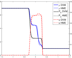
(a) M=1 RHD

(b) M=2

(c) M=3

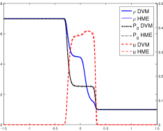
(d) M=4

(e) M=5

(f) M=6

(g) M=7

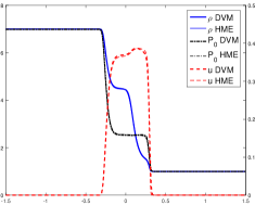
(h) M=8

(i) M=9

Figure 6.1: Numerical results of the shock tube problem for $Kn=0.05$. The left $y$-axis is for $\rho$ and $P_{0}$, and the right $y$-axis is for $u$. The thin lines are the numerical results of the HME (4.20), and the thick lines are the results of DVM. The solid blue lines denote $\rho$, dashed red lines denote $u$, and dash-dotted black lines denote $P_{0}$.

The results at $t=0.3$ for the case of $Kn=0.5$ are shown in Fig. 6.2. The discontinuities are clearer than the case of $Kn=0.05$ when $M=1,2,\cdots 9$, and the convergence of the moment method can also be readily observed, but it is slower than the case of $Kn=0.05$. The contact discontinuities and shock waves are obvious when $M\leq 2$, but when $M>6$, the discontinuities are fully damped and the solutions are almost the same as the reference solutions.

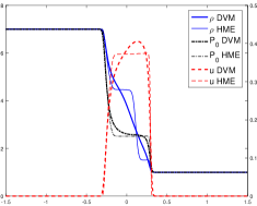
(a) M=1 RHD

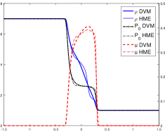
(b) M=2

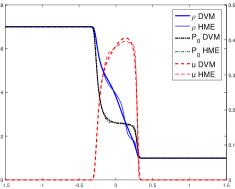
(c) M=3

(d) M=4

(e) M=5

(f) M=6

(g) M=7

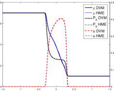
(h) M=8

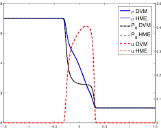
(i) M=9

Figure 6.2: Same as Fig. 6.1 except for $Kn=0.5$.

7 Conclusions

The paper derived the arbitrary order globally hyperbolic moment system of the one-dimensional (1D) special relativistic Boltzmann equation for the first time and studied the properties of the moment system: the eigenvalues and their bound as well as eigenvectors, hyperbolicity, characteristic fields, linear stability, and Lorentz covariance. The key contribution was the careful study of two families of the complicate Grad type orthogonal polynomials depending on a parameter. We derived the recurrence relations and derivative relations with respect to the independent variable and the parameter respectively, and studied their zeros and coefficient matrices in the recurrence formulas. Built on the knowledges of two families of the Grad type orthogonal polynomials with a parameter, the model reduction method by the operator projection MR:2014 might be extended to the 1D special relativistic Boltzmann equation.

A semi-implicit operator-splitting type numerical scheme was presented for our hyperbolic moment system and a Cauchy problem was solved to verify the convergence behavior of the moment method in comparison with the discrete velocity method. The results showed that the solutions of our hyperbolic moment system could converge to the solution of the special relativistic Boltzmann equation as the order of the hyperbolic moment system increases.

Now we are deriving the globally hyperbolic moment model of arbitrary order for the 3D special relativistic Boltzmann equation. Moreover, it is interesting to develop robust, high order accurate numerical schemes for the moment system and find other basis for the derivation of moment system with some good property, e.g. non-negativity.

Appendix A Proofs in Section 2

A.1 Proof of Theorem 2.1

Proof

For the nonnegative distribution $f(x,p,t)$, which is not identically zero, using (2.3) gives

$$T^{\alpha\alpha}>0,\alpha=0,1;\quad T^{00}+T^{11}{\pm}2T^{01}={c}\int_{\mathbb{R}}(p^{0}{\pm}p^{1})^{2}f\frac{dp}{p^{0}}>0,$$

which implies the first inequality in (2.22).

Using the definition of $\Delta^{\alpha\beta}$ in (2.6) and the tensor decomposition of $T^{\alpha\beta}$ in (2.5) gives (2.23), which is a quadratic equation with respect to $u$. The first inequality in (2.22) tells us that (2.23) has two different solutions whose product is equal to ${c^{2}}$, while one of them with a smaller absolute value is (2.24).

Using further (2.3) gives

$${N^{0}-c^{-1}uN^{1}=c\int_{\mathbb{R}}(p^{0}-c^{-1}up^{1})f\frac{dp}{p^{0}}}>0,$$

i.e. the second inequality in (2.22), and then using the tensor decomposition of $N^{\alpha}$ in (2.4) gives

$$\rho={c^{-1}m\frac{N^{0}-c^{-1}uN^{1}}{\sqrt{1-c^{-2}u^{2}}}}>0.$$

Using the second identity in (2.17), the expression of $\varepsilon_{0}$ in (2.20), and (2.5) gives (2.26).

And the inequality ${E\geq mc^{2}}$ holds because

$$E=U_{\alpha}p^{\alpha}={(1-c^{-2}u^{2})^{-\frac{1}{2}}\left(c\sqrt{m^{2}c^{2}+p^{2}}-up\right)}>0,$$

and

$${E^{2}-m^{2}c^{4}=(1-c^{-2}u^{2})^{-1}(u\sqrt{m^{2}c^{2}+p^{2}}-cp)^{2}=\left(\frac{c^{2}}{U^{0}}p_{<1>}\right)^{2}}\geq 0.$$

Thus

$${T^{00}-c^{-1}uT^{01}-c^{2}\rho=\frac{T^{00}-2c^{-1}uT^{01}+c^{-2}u^{2}T^{11}}{1-c^{-2}u^{2}}-c^{2}\rho=c^{-1}\int_{\mathbb{R}}E(E-mc^{2})f\frac{dp^{1}}{p^{0}}}>0,$$

the third inequality in (2.22) holds, and thus implies that $G(\theta^{-1})-\theta>1$ for $\theta\in(0,+\infty)$.

On the other hand, one has

$$\lim_{\theta\rightarrow 0}\left(G(\theta^{-1})-\theta\right)=1,\ \lim_{\theta\rightarrow+\infty}\left(G(\theta^{-1})-\theta\right)=\lim_{\theta\rightarrow+\infty}\theta=+\infty,$$

and

$$\frac{\partial(G(\theta^{-1})-\theta)}{\partial\theta}= -\theta^{-2}\left(G(\theta^{-1})^{2}-3G(\theta^{-1})\theta+\theta^{2}-1\right)=:\tilde{\psi}(G(\theta^{-1}),\theta).$$

Because

$$0 <c^{-1}\int_{\mathbb{R}}(E-mc^{2})f^{(0)}\frac{dp}{p^{0}}=-m^{-1}\rho(G(\theta^{-1})-2\theta-1),$$

$$0 <c^{-1}\int_{\mathbb{R}}(E-mc^{2})^{2}f^{(0)}\frac{dp}{p^{0}}=\rho c^{2}(2G(\theta^{-1})-3\theta-2),$$

$$0 <c^{-1}\int_{\mathbb{R}}(E-mc^{2})^{3}f^{(0)}\frac{dp}{p^{0}}=-\rho mc^{4}((4-\theta)G(\theta^{-1})-5\theta-4),$$

one obtains

$$\frac{3}{2}\theta+1<G(\theta^{-1})<\begin{cases}\min\left\{2\theta+1,(4-\theta)^{-1}(5\theta+4)\right\},&0<\theta<4,\\ 2\theta+1,&\theta\geq 4,\end{cases}$$

which is equivalent to the following inequality

$$\frac{3}{2}\theta+1 <G(\theta^{-1})<\begin{cases}(4-\theta)^{-1}(5\theta+4),&0<\theta<1,\\ 2\theta+1,&\theta\geq 1.\end{cases}$$

Thus, one has

$$\tilde{\psi}(G(\theta^{-1}),\theta)>\begin{cases}\tilde{\psi}\left(2\theta+1,\theta\right)>\theta^{3}(\theta-1)>0,&\theta\geq 1,\\ \\ \tilde{\psi}\left((4-\theta)^{-1}(5\theta+4),\theta\right)>(4-\theta)^{-2}\theta^{4}(\theta+8)(1-\theta)>0,&\theta<1,\end{cases}$$

i.e.

$$\frac{\partial(G(\theta^{-1})-\theta)}{\partial\theta}>0,$$

which implies that $G(\theta^{-1})-\theta$ is a strictly monotonic function of $\theta$ in the interval $(0,+\infty)$.

Thus (2.26) has a unique solution in the interval $(0,+\infty)$. The proof is completed. ∎

A.2 Proof of Theorem 2.2

Proof

Under Theorem 2.1, for the nonnegative distribution $f(x,p,t)$, which is not identically zero, one obtains $\{\rho,u,\theta\}$ satisfying

$$\rho>0,\quad|u|<{c},\quad\theta>0.$$ (A.1)

Due to the last equations in (2.7) and (2.20), one obtains

$${\Pi=-\int_{\mathbb{R}}\Delta_{\alpha\beta}p^{\alpha}p^{\beta}f\frac{dp}{p^{0}}-c^{2}\rho\theta=c^{-1}\int_{\mathbb{R}}(E^{2}-m^{2}c^{4})f\frac{dp}{p^{0}}-\rho c^{2}\theta>-\rho c^{2}\theta},$$

which completes the proof. ∎

Appendix B Proofs in Section 3

B.1 Proof of Theorem 3.2

Proof

(i) For $k\leq n+2$, taking the inner product with respect to $\omega^{(0)}$ between the polynomials $P_{k}^{(0)}(x;\zeta)$ and $(x^{2}-1)P_{n}^{(1)}(x;\zeta)$ gives

$$\left((x^{2}-1)P_{n}^{(1)},P_{n+2}^{(0)}\right)_{\omega^{(0)}} =\left(c_{n}^{(1)}x^{n+2},P_{n+2}^{(0)}\right)_{\omega^{(0)}}=\frac{c_{n}^{(1)}}{c_{n+2}^{(0)}}\left(P_{n+2}^{(0)},P_{n+2}^{(0)}\right)_{\omega^{(0)}}=r_{n+1},$$

$$\left((x^{2}-1)P_{n}^{(1)},P_{n+1}^{(0)}\right)_{\omega^{(0)}} =\left(c_{n}^{(1)}\left(x^{n+2}-\sum_{i=1}^{n+2}x_{i,n+2}^{(0)}x^{n+1}+\left(\sum_{i=1}^{n+2}x_{i,n+2}^{(0)}-\sum_{i=1}^{n}x_{i,n}^{(1)}\right)x^{n+1}\right),P_{n+1}^{(0)}\right)_{\omega^{(0)}}$$

$$=r_{n+1}\left(P_{n+2}^{(0)},P_{n+1}^{(0)}\right)_{\omega^{(0)}}+q_{n}\left(P_{n+1}^{(0)},P_{n+1}^{(0)}\right)_{\omega^{(0)}}=q_{n},$$

$$\left((x^{2}-1)P_{n}^{(1)},P_{n+1}^{(0)}\right)_{\omega^{(0)}} =\left(P_{n}^{(1)},c_{n+1}^{(0)}\left(x^{n+1}-\sum_{i=1}^{n+1}x_{i,n+1}^{(1)}x^{n}+\left(\sum_{i=1}^{n+1}x_{i,n+1}^{(1)}-\sum_{i=1}^{n+1}x_{i,n+1}^{(0)}\right)x^{n}\right)\right)_{\omega^{(1)}}$$

$$=p_{n+1}\left(P_{n}^{(1)},P_{n+1}^{(1)}\right)_{\omega^{(1)}}+\frac{c_{n+1}^{(0)}}{c_{n}^{(1)}}\left(\sum_{i=1}^{n+1}x_{i,n+1}^{(1)}-\sum_{i=1}^{n+1}x_{i,n+1}^{(0)}\right)\left(P_{n}^{(1)},P_{n}^{(1)}\right)_{\omega^{(1)}}$$

$$=\frac{c_{n+1}^{(0)}}{c_{n}^{(1)}}\sum_{i=1}^{n+1}\left(x_{i,n+1}^{(1)}-x_{i,n+1}^{(0)}\right)=q_{n},$$

$$\left((x^{2}-1)P_{n}^{(1)},P_{n}^{(0)}\right)_{\omega^{(0)}} =\left(P_{n}^{(1)},P_{n}^{(0)}\right)_{\omega^{(1)}}=\left(P_{n}^{(1)},c_{n}^{(0)}x^{n}\right)_{\omega^{(1)}}=p_{n}\left(P_{n}^{(1)},P_{n}^{(1)}\right)_{\omega^{(1)}}=p_{n},$$

$$\left((x^{2}-1)P_{n}^{(1)},P_{k}^{(0)}\right)_{\omega^{(0)}} =\left(P_{n}^{(1)},P_{k}^{(0)}\right)_{\omega^{(1)}}=0,\quad k\leq n-1,$$

Substituting them into (3.3) gives (3.9).

(ii) Taking the inner product with respect to $\omega^{(1)}$ between $P_{n+1}^{(0)}(x;\zeta)$ and $P_{k}^{(1)}(x;\zeta)$ with $k\leq n+1$

$$\left(P_{n+1}^{(0)},P_{n+1}^{(1)}\right)_{\omega^{(1)}} =\left(c_{n+1}^{(0)}x^{n+1},P_{n+1}^{(1)}\right)_{\omega^{(1)}}=p_{n+1}\left(P_{n+1}^{(1)},P_{n+1}^{(1)}\right)_{\omega^{(1)}}=p_{n+1},$$

$$\left(P_{n+1}^{(0)},P_{n}^{(1)}\right)_{\omega^{(1)}} =\left(P_{n+1}^{(0)},(x^{2}-1)P_{n}^{(1)}\right)_{\omega^{(0)}}=q_{n},$$

$$\left(P_{n+1}^{(0)},P_{n-1}^{(1)}\right)_{\omega^{(1)}} =\left(P_{n+1}^{(0)},(x^{2}-1)P_{n-1}^{(1)}\right)_{\omega^{(0)}}=r_{n}\left(P_{n+1}^{(0)},P_{n+1}^{(0)}\right)_{\omega^{(0)}}=r_{n},$$

$$\left(P_{n+1}^{(0)},P_{k}^{(1)}\right)_{\omega^{(1)}} =\left(P_{n+1}^{(0)},(x^{2}-1)P_{k}^{(1)}\right)_{\omega^{(0)}}=0,\quad k\leq n-2.$$

Similarly, substituting them into (3.3) gives (3.10).

(iii) If using (3.6) to eliminate $P_{n+2}^{(0)}$ and $P_{n+1}^{(1)}$ in (3.9) and (3.10) respectively, then one obtains

$$(x^{2}-1)P_{n}^{(1)}=\tilde{p}_{n}(x+\tilde{q}_{n})P_{n+1}^{(0)}+\tilde{r}_{n}P_{n}^{(0)},\quad P_{n+1}^{(0)}=\frac{1}{\tilde{\tilde{p}}_{n}}(x-\tilde{\tilde{q}}_{n})P_{n}^{(1)}-\frac{a_{n-1}^{(1)}}{a_{n}^{(0)}}\tilde{\tilde{r}}_{n}P_{n-1}^{(1)},$$

with

$$\tilde{p}_{n}=\frac{r_{n+1}}{a_{n+1}^{(0)}}=\frac{c_{n}^{(1)}}{c_{n+1}^{(0)}}=\frac{a_{n}^{(1)}}{p_{n+1}}=\tilde{\tilde{p}}_{n},$$

$$\tilde{q}_{n}=\frac{1}{\tilde{p}_{n}}q_{n}-b_{n+1}^{(0)}=\sum_{i=1}^{n+1}x_{i,n+1}^{(0)}-\sum_{i=1}^{n}x_{i,n}^{(1)}=b_{n}^{(1)}-\tilde{p}_{n}q_{n}=\tilde{\tilde{q}}_{n},$$

$$\tilde{r}_{n}=p_{n}-\tilde{p}_{n}a_{n}^{(0)}={p_{n}(1-\tilde{p}_{n}^{2})}=\frac{a_{n}^{(0)}}{a_{n-1}^{(1)}}\left(-r_{n}+\frac{1}{\tilde{p}_{n}}a_{n-1}^{(1)}\right)=\tilde{\tilde{r}}_{n}.$$

The proof is completed. ∎

B.2 Proof of Theorem 3.3

Proof

With the aid of definition and recurrence relation of the second kind modified Bessel function in (2.18) and (2.19), one has

$$\frac{\partial}{\partial\zeta}\omega^{(\ell)}(x;\zeta) =\frac{K_{2}(\zeta)+K_{0}(\zeta)-2xK_{1}(\zeta)}{2K_{1}(\zeta)}\left(\frac{1}{K_{1}(\zeta)}(x^{2}-1)^{\ell-\frac{1}{2}}\exp(-\zeta x)\right)$$

$$=\left(G(\zeta)-\zeta^{-1}-x\right)\omega^{(\ell)}(x;\zeta).$$

Taking the partial derivative of both sides of identities

$$\left(P_{n+1}^{(\ell)},P_{k}^{(\ell)}\right)_{\omega^{(\ell)}}=\delta_{n+1,k},k=0,\cdots,n+1,$$

with respect to $\zeta$ and using (3.8) gives

$$\frac{\partial}{\partial\zeta}\left(P_{n+1}^{(\ell)},P_{n+1}^{(\ell)}\right)_{\omega^{(\ell)}}= 2\left(\frac{\partial}{\partial\zeta}P_{n+1}^{(\ell)},P_{n+1}^{(\ell)}\right)_{\omega^{(\ell)}}+\left(G(\zeta)-\zeta^{-1}\right)\left(P_{n+1}^{(\ell)},P_{n+1}^{(\ell)}\right)_{\omega^{(\ell)}}-\left(xP_{n+1}^{(\ell)},P_{n+1}^{(\ell)}\right)_{\omega^{(\ell)}}$$

$$= 2\left(\frac{\partial}{\partial\zeta}P_{n+1}^{(\ell)},P_{n+1}^{(\ell)}\right)_{\omega^{(\ell)}}+\left(G(\zeta)-\zeta^{-1}-b_{n+1}^{(\ell)}\right)=0,$$

$$\frac{\partial}{\partial\zeta}\left(P_{n+1}^{(\ell)},P_{n}^{(\ell)}\right)_{\omega^{(\ell)}}= \left(\frac{\partial}{\partial\zeta}P_{n+1}^{(\ell)},P_{n}^{(\ell)}\right)_{\omega^{(\ell)}}+\left(P_{n+1}^{(\ell)},\frac{\partial}{\partial\zeta}P_{n}^{(\ell)}\right)_{\omega^{(\ell)}}$$

$$+\left(G(\zeta)-\zeta^{-1}\right)\left(P_{n+1}^{(\ell)},P_{n}^{(\ell)}\right)_{\omega^{(\ell)}}-\left(xP_{n}^{(\ell)},P_{n+1}^{(\ell)}\right)_{\omega^{(\ell)}}$$

$$= \left(\frac{\partial}{\partial\zeta}P_{n+1}^{(\ell)},P_{n}^{(\ell)}\right)_{\omega^{(\ell)}}-a_{n}^{(\ell)}=0,$$

$$\frac{\partial}{\partial\zeta}\left(P_{n+1}^{(\ell)},P_{k}^{(\ell)}\right)_{\omega^{(\ell)}}= \left(\frac{\partial}{\partial\zeta}P_{n+1}^{(\ell)},P_{k}^{(\ell)}\right)_{\omega^{(\ell)}}+\left(P_{n+1}^{(\ell)},\frac{\partial}{\partial\zeta}P_{k}^{(\ell)}\right)_{\omega^{(\ell)}}$$

$$+\left(G(\zeta)-\zeta^{-1}\right)\left(P_{n+1}^{(\ell)},P_{k}^{(\ell)}\right)_{\omega^{(\ell)}}-\left(xP_{k}^{(\ell)},P_{n+1}^{(\ell)}\right)_{\omega^{(\ell)}}$$

$$= \left(\frac{\partial}{\partial\zeta}P_{n+1}^{(\ell)},P_{k}^{(\ell)}\right)_{\omega^{(\ell)}}=0,\quad k\leq n-1.$$

Thus one has

$$\left(\frac{\partial}{\partial\zeta}P_{n+1}^{(\ell)},P_{n+1}^{(\ell)}\right)_{\omega^{(\ell)}} =-\frac{1}{2}\left(G(\zeta)-\zeta^{-1}-b_{n+1}^{(\ell)}\right),$$

$$\left(\frac{\partial}{\partial\zeta}P_{n+1}^{(\ell)},P_{n}^{(\ell)}\right)_{\omega^{(\ell)}} =a_{n}^{(\ell)},\quad\left(\frac{\partial}{\partial\zeta}P_{n+1}^{(\ell)},P_{k}^{(\ell)}\right)_{\omega^{(\ell)}}=0,\quad k\leq n-1.$$

Because $\frac{\partial P_{n+1}^{(\ell)}}{\partial\zeta}$ is a polynomial and its degree is not larger than $n+1$, using (3.3) gives (3.17). The proof is completed. ∎

B.3 Proof of Theorem 3.4

Proof

Similar to the proof of Theorem 3.3, one has

$${\frac{\partial}{\partial x}\omega^{(1)}(x;\zeta)=x\omega^{(0)}(x;\zeta)-\zeta\omega^{(1)}(x;\zeta).}$$

Because the degrees of polynomials $\frac{\partial P_{n+1}^{(0)}}{\partial x}$ and $(x^{2}-1)\frac{\partial P_{n}^{(1)}}{\partial x}+xP_{n}^{(1)}$ are not larger than $n$ and $n+1$, respectively, and

$$\lim_{x\rightarrow+\infty}P_{i}^{(0)}(x;\zeta)P_{j}^{(1)}(x;\zeta)\omega^{(1)}(x;\zeta)=0,\quad\lim_{x\rightarrow 1}P_{i}^{(0)}(x;\zeta)P_{j}^{(1)}(x;\zeta)\omega^{(1)}(x;\zeta)=0,\quad\forall i,j\in\mathbb{N},$$

one can calculate the expansion coefficients in (3.3) as follows

$$\left(\frac{\partial}{\partial x}P_{n+1}^{(0)},P_{n}^{(1)}\right)_{\omega^{(1)}}= \left((n+1)c_{n+1}^{(0)}x^{n},P_{n}^{(1)}\right)_{\omega^{(1)}}=\frac{n+1}{\tilde{p}_{n}}\left(P_{n}^{(1)},P_{n}^{(1)}\right)_{\omega^{(1)}}=\frac{n+1}{\tilde{p}_{n}},$$

$$\left(\frac{\partial}{\partial x}P_{n+1}^{(0)},P_{n-1}^{(1)}\right)_{\omega^{(1)}}= \int_{1}^{+\infty}\frac{\partial}{\partial x}\left(P_{n+1}^{(0)}P_{n-1}^{(1)}\omega^{(1)}\right)dx-\left(P_{n+1}^{(0)},(x^{2}-1)\frac{\partial}{\partial x}P_{n-1}^{(1)}\right)_{\omega^{(0)}}$$

$$-\left(P_{n+1}^{(0)},xP_{n-1}^{(1)}\right)_{\omega^{(0)}}+\zeta\left(P_{n+1}^{(0)},(x^{2}-1)P_{n-1}^{(1)}\right)_{\omega^{(0)}}=\zeta r_{n},$$

$$\left(\frac{\partial}{\partial x}P_{n+1}^{(0)},P_{k}^{(1)}\right)_{\omega^{(1)}}= \int_{1}^{+\infty}\frac{\partial}{\partial x}\left(P_{n+1}^{(0)}P_{k}^{(1)}\omega^{(1)}\right)dx-\left(P_{n+1}^{(0)},(x^{2}-1)\frac{\partial}{\partial x}P_{k}^{(1)}\right)_{\omega^{(0)}}$$

$$-\left(P_{n+1}^{(0)},xP_{k}^{(1)}\right)_{\omega^{(0)}}+\zeta\left(P_{n+1}^{(0)},(x^{2}-1)P_{k}^{(1)}\right)_{\omega^{(0)}}=0,k\leq n-2.$$

and

$$\left((x^{2}-1)\frac{\partial}{\partial x}P_{n}^{(1)}+xP_{n}^{(1)},P_{n+1}^{(0)}\right)_{\omega^{(0)}}= \left((n+1)c_{n}^{(1)}x^{n+1},P_{n+1}^{(0)}\right)_{\omega^{(0)}}$$

$$= (n+1)\tilde{p}_{n}\left(P_{n+1}^{(0)},P_{n+1}^{(0)}\right)_{\omega^{(0)}}=(n+1)\tilde{p}_{n},$$

$$\left((x^{2}-1)\frac{\partial}{\partial x}P_{n}^{(1)}+xP_{n}^{(1)},P_{n}^{(0)}\right)_{\omega^{(0)}}= \int_{1}^{+\infty}\frac{\partial}{\partial x}\left(P_{n}^{(1)}P_{n}^{(0)}\omega^{(1)}\right)dx-\left(P_{n}^{(1)},\frac{\partial}{\partial x}P_{n}^{(0)}\right)_{\omega^{(1)}}$$

$$+\zeta\left(P_{n}^{(1)},P_{n}^{(0)}\right)_{\omega^{(1)}}=\zeta\left(P_{n}^{(1)},P_{n}^{(0)}\right)_{\omega^{(1)}}=\zeta p_{n},$$

$$\left((x^{2}-1)\frac{\partial}{\partial x}P_{n}^{(1)}+xP_{n}^{(1)},P_{k}^{(0)}\right)_{\omega^{(0)}}= \int_{1}^{+\infty}\frac{\partial}{\partial x}\left(P_{n}^{(1)}P_{k}^{(0)}\omega^{(1)}\right)dx-\left(P_{n}^{(1)},\frac{\partial}{\partial x}P_{k}^{(0)}\right)_{\omega^{(1)}}$$

$$+\zeta\left(P_{n}^{(1)},P_{k}^{(0)}\right)_{\omega^{(1)}}=0,k\leq n-1.$$

The proof is completed. ∎

B.4 Proof of Theorem 3.6

Proof

Substituting $\{x_{i,n+1}^{(0)}\}_{i=1}^{n+1}$ into (3.14) gives

$$\left((x_{i,n+1}^{(0)})^{2}-1\right)P_{n}^{(1)}(x_{i,n+1}^{(0)};\zeta)=\tilde{r}_{n}P_{n}^{(0)}(x_{i,n+1}^{(0)};\zeta).$$

which implies that $\tilde{r}_{n}\neq 0$. In fact, if assuming $\tilde{r}_{n}=0$, then the above identity and the fact that $(x_{i,n+1}^{(0)})^{2}-1>0$ imply $P_{n}^{(1)}(x_{i,n+1}^{(0)};\zeta)=0$, which contradicts with $P_{n}^{(1)}$ being a polynomial of degree $n$.

Using Theorem 3.5 gives

$${\rm sign}\left(P_{n}^{(1)}(x_{i,n+1}^{(0)};\zeta)P_{n}^{(1)}(x_{i+1,n+1}^{(0)};\zeta)\right)={\rm sign}\left(P_{n}^{(0)}(x_{i,n+1}^{(0)};\zeta)P_{n}^{(0)}(x_{i+1,n+1}^{(0)};\zeta)\right)<0.$$

Thus there exist no less than one zero of the polynomial $P_{n}^{(1)}$ in each subinterval $\left(x_{i,n+1}^{(0)},x_{i+1,n+1}^{(0)}\right)$. The proof is completed. ∎

B.5 Proof of Corollary 1

Proof

It is obvious that

$$p_{n}=\frac{c_{n}^{(0)}}{c_{n}^{(1)}}>0,\quad r_{n}=\frac{c_{n-1}^{(1)}}{c_{n+1}^{(0)}}>0,\quad\tilde{p}_{n}=\frac{c_{n}^{(1)}}{c_{n+1}^{(0)}}>0.$$

Using Theorems 3.1 and 3.6 gives

$$\tilde{q}_{n} =\sum_{i=1}^{n+1}x_{i,n+1}^{(0)}-\sum_{i=1}^{n}x_{i,n}^{(1)}=\sum_{i=1}^{n}\left(x_{i+1,n+1}^{(0)}-x_{i,n}^{(1)}\right)+x_{1,n+1}^{(0)}>0,$$

$$q_{n} =\tilde{p}_{n}\left(\sum_{i=1}^{n+2}x_{i,n+2}^{(0)}-\sum_{i=1}^{n}x_{i,n}^{(1)}\right)=\tilde{p}_{n}\left(b_{n+1}^{(0)}+\tilde{q}_{n}\right)>0,$$

which imply $q_{n}>0$ and $\tilde{q}_{n}>0$.

Comparing the coefficients of the term of order $n$ at two sides of (3.14) gives

$$\tilde{r}_{n}=p_{n}^{-1}\left(\sum_{i=1}^{n}\sum_{j=i+1}^{n}x_{i,n}^{(1)}x_{j,n}^{(1)}-1-\sum_{i=1}^{n+1}\sum_{j=i+1}^{n+1}x_{i,n+1}^{(0)}x_{j,n+1}^{(0)}+\left(\sum_{i=1}^{n+1}x_{i,n+1}^{(0)}-\sum_{i=1}^{n}x_{i,n}^{(1)}\right)\sum_{i=1}^{n+1}x_{i,n+1}^{(0)}\right)$$

$$=p_{n}^{-1}\left(\sum_{i=1}^{n}\sum_{j=i+1}^{n}x_{i,n}^{(1)}x_{j,n}^{(1)}+\sum_{i=1}^{n+1}\sum_{j=i}^{n+1}x_{i,n+1}^{(0)}x_{j,n+1}^{(0)}-\sum_{i=1}^{n}x_{i,n}^{(1)}\sum_{i=1}^{n+1}x_{i,n+1}^{(0)}-1\right)$$

$$=p_{n}^{-1}\left(\sum_{i=1}^{n}x_{i+1,n+1}^{(0)}(x_{i+1,n+1}^{(0)}-x_{i,n}^{(1)})+(x_{1,n+1}^{(0)})^{2}-1+\sum_{i=0}^{n}\sum_{j=i+1}^{n}(x_{i+1,n+1}^{(0)}-x_{i,n}^{(1)})(x_{j+1,n+1}^{(0)}-x_{j,n}^{(1)})\right),$$

where $x_{0,n}^{(1)}=0$.

Combining Theorem 3.6 gives $\tilde{r}_{n}>0$. The proof is completed. ∎

B.6 Proof of Corollary 3

Proof

Taking partial derivative of $P_{n}^{(\ell)}(x_{i,n}^{(\ell)};\zeta)$ with respect to $\zeta$ and using Theorem 3.3 gives

$$\frac{\partial x_{i,n}^{(\ell)}}{\partial\zeta}=-\left(\frac{\partial P_{n}^{(\ell)}}{\partial x}(x_{i,n}^{(\ell)};\zeta)\right)^{-1}\left(\frac{\partial P_{n}^{(\ell)}}{\partial\zeta}(x_{i,n}^{(\ell)};\zeta)\right)=-a_{n-1}^{(\ell)}\left(\frac{\partial P_{n}^{(\ell)}}{\partial x}(x_{i,n}^{(\ell)};\zeta)\right)^{-1}P_{n-1}^{(\ell)}(x_{i,n}^{(\ell)};\zeta).$$

Due to Theorem 3.5, one has

$${\rm sign}(P_{n-1}^{(\ell)}(x_{i,n}^{(\ell)};\zeta))=(-1)^{n+i}={\rm sign}\left(\frac{\partial P_{n}^{(\ell)}}{\partial x}(x_{i,n}^{(\ell)};\zeta)\right).$$

Combining them completes the proof. ∎

B.7 Proof of Lemma 1

Proof

According to the definition of $Q_{2n}(x;\zeta)$ in (3.30), it is not difficult to know that $Q_{2n}(x;\zeta)$ is an even function and a polynomial of degree $2n$.

If taking $x$ in (3.30) as the zero of $P_{n+1}^{(0)}(x;\zeta)$, i.e. $x=x_{i,n+1}^{(0)}$, $i=1,\cdots,{n+1}$, then one has

$$Q_{2n}(x_{i,n+1}^{(0)};\zeta)=P_{n+1}^{(0)}(-x_{i,n+1}^{(0)};\zeta)P_{n}^{(1)}(x_{i,n+1}^{(0)};\zeta).$$

Since

$${\rm sign}\left(P_{n+1}^{(0)}(-x_{i,n+1}^{(0)};\zeta)\right)=(-1)^{n+1},\quad i=1,\cdots,n+1,$$

using Theorem 3.6 gives

$${\rm sign}\left(Q_{2n}(x_{i,n+1}^{(0)};\zeta)Q_{2n}(x_{i+1,n+1}^{(0)};\zeta)\right)={\rm sign}\left(P_{n}^{(1)}(x_{i,n+1}^{(0)};\zeta)P_{n}^{(1)}(x_{i+1,n+1}^{(0)};\zeta)\right)<0,$$

for $i=1,\cdots,n$, which implies that there exist no less than one zero of $Q_{2n}(x;\zeta)$ in each subinterval $(x_{i,n+1}^{(0)},x_{i+1,n+1}^{(0)})$, $i=1,\cdots,n$. Because $Q_{2n}(x;\zeta)$ is an even polynomial of degree $2n$, there exists exactly one zero of $Q_{2n}(x;\zeta)$ in each subinterval $(x_{i,n+1}^{(0)},x_{i+1,n+1}^{(0)})$, $i=1,\cdots,n$. The proof is completed. ∎

B.8 Proof of Lemma 2

Proof

According to the definition of $Q_{2n}(x;\zeta)$ in (3.30), one has

$$\frac{\partial Q_{2n}}{\partial\zeta}(z_{i,n};\zeta)= \frac{\partial P_{n+1}^{(0)}}{\partial\zeta}\Big{|}_{x=z_{i,n}}P_{n}^{(1)}(-z_{i,n};\zeta)+\frac{\partial P_{n}^{(1)}}{\partial\zeta}\Big{|}_{x=z_{i,n}}P_{n+1}^{(0)}(-z_{i,n};\zeta)$$

$$+\frac{\partial P_{n+1}^{(0)}}{\partial\zeta}\Big{|}_{x=-z_{i,n}}P_{n}^{(1)}(z_{i,n};\zeta)+\frac{\partial P_{n}^{(1)}}{\partial\zeta}\Big{|}_{x=-z_{i,n}}P_{n+1}^{(0)}(z_{i,n};\zeta).$$

Using Theorem 3.3 gives

$$\frac{\partial Q_{2n}}{\partial\zeta}(z_{i,n};\zeta)= a_{n}^{(0)}\left(P_{n}^{(0)}(z_{i,n};\zeta)P_{n}^{(1)}(-z_{i,n};\zeta)+P_{n}^{(0)}(-z_{i,n};\zeta)P_{n}^{(1)}(z_{i,n};\zeta)\right)$$

$$+a_{n-1}^{(1)}\left(P_{n-1}^{(1)}(z_{i,n};\zeta)P_{n+1}^{(0)}(-z_{i,n};\zeta)+P_{n-1}^{(1)}(-z_{i,n};\zeta)P_{n+1}^{(0)}(z_{i,n};\zeta)\right)$$

$$+\left(\frac{1}{2}(b_{n+1}^{(0)}+b_{n}^{(1)})-(G(\zeta)-\zeta^{-1})\right)Q_{2n}(z_{i,n};\zeta)$$

$$= a_{n}^{(0)}\left(P_{n}^{(0)}(z_{i,n};\zeta)P_{n}^{(1)}(-z_{i,n};\zeta)+P_{n}^{(0)}(-z_{i,n};\zeta)P_{n}^{(1)}(z_{i,n};\zeta)\right)$$

$$+a_{n-1}^{(1)}\left(P_{n-1}^{(1)}(z_{i,n};\zeta)P_{n+1}^{(0)}(-z_{i,n};\zeta)+P_{n-1}^{(1)}(-z_{i,n};\zeta)P_{n+1}^{(0)}(z_{i,n};\zeta)\right).$$

Substituting (3.14) and (3.15) into it gives

$$\frac{\partial Q_{2n}}{\partial\zeta}(z_{i,n};\zeta)= \frac{2a_{n}^{(0)}}{\tilde{r}_{n}}\left(((z_{i,n})^{2}-1)P_{n}^{(1)}(z_{i,n};\zeta)P_{n}^{(1)}(-z_{i,n};\zeta)+\tilde{p}_{n}z_{i,n}P_{n+1}^{(0)}(-z_{i,n};\zeta)P_{n}^{(1)}(z_{i,n};\zeta)\right)$$

$$-\frac{2a_{n}^{(0)}}{\tilde{r}_{n}}\left(P_{n+1}^{(0)}(z_{i,n};\zeta)P_{n+1}^{(0)}(-z_{i,n};\zeta)-\tilde{p}_{n}^{-1}z_{i,n}P_{n+1}^{(0)}(-z_{i,n};\zeta)P_{n}^{(1)}(z_{i,n};\zeta)\right)$$

$$= 2\frac{P_{n}^{(1)}(z_{i,n};\zeta)}{P_{n}^{(1)}(-z_{i,n};\zeta)}\frac{a_{n}^{(0)}}{\tilde{r}_{n}}\left((\tilde{p}_{n}+\tilde{p}_{n}^{-1})z_{i,n}P_{n}^{(1)}(-z_{i,n};\zeta)P_{n+1}^{(0)}(-z_{i,n};\zeta)\right.$$

$$\left.+(z_{i,n}^{2}-1)P_{n}^{(1)}(-z_{i,n};\zeta)^{2}+P_{n+1}^{(0)}(-z_{i,n};\zeta)^{2}\right)$$

$$= 2\frac{P_{n}^{(1)}(z_{i,n};\zeta)}{P_{n}^{(1)}(-z_{i,n};\zeta)}\frac{a_{n}^{(0)}}{\tilde{r}_{n}}\left((c_{n+1}^{(0)})^{2}\prod_{j=1}^{n+1}(z_{i,n}+x_{j,n+1}^{(0)})\tilde{I}_{1}-(c_{n}^{(1)})^{2}\prod_{j=1}^{n}(z_{i,n}+x_{j,n}^{(1)})\tilde{I}_{2}\right),$$

where

$$\tilde{I}_{1}:=\prod_{j=1}^{n+1}(z_{i,n}+x_{j,n+1}^{(0)})-z_{i,n}\prod_{j=1}^{n}(z_{i,n}+x_{j,n}^{(1)}),$$

$$\tilde{I}_{2}:=z_{i,n}\prod_{j=1}^{n+1}(z_{i,n}+x_{j,n+1}^{(0)})-(z_{i,n}^{2}-1)\prod_{j=1}^{n}(z_{i,n}+x_{j,n}^{(1)}).$$

Similarly, using Theorem 3.4 and (3.14)-(3.15) gives

$$\frac{\partial Q_{2n}}{\partial x}(z_{i,n};\zeta)= \zeta\frac{c_{n-1}^{(1)}}{c_{n+1}^{(0)}}\left(P_{n-1}^{(1)}(z_{i,n};\zeta)P_{n}^{(1)}(-z_{i,n};\zeta)-P_{n-1}^{(1)}(-z_{i,n};\zeta)P_{n}^{(1)}(z_{i,n};\zeta)\right)$$

$$+(z_{i,n}^{2}-1)^{-1}\zeta\frac{c_{n}^{(0)}}{c_{n}^{(1)}}\left(P_{n}^{(0)}(z_{i,n};\zeta)P_{n+1}^{(0)}(-z_{i,n};\zeta)-P_{n}^{(0)}(-z_{i,n};\zeta)P_{n+1}^{(0)}(z_{i,n};\zeta)\right)$$

$$= 2\zeta\frac{P_{n}^{(1)}(z_{i,n};\zeta)}{P_{n}^{(1)}(-z_{i,n};\zeta)}\frac{a_{n}^{(0)}}{\tilde{r}_{n}}\left(z_{i,n}P_{n}^{(1)}(-z_{i,n};\zeta)^{2}\right.$$

$$\left.+(\tilde{p}_{n}+\tilde{p}_{n}^{-1})P_{n+1}^{(0)}(-z_{i,n};\zeta)P_{n}^{(1)}(-z_{i,n};\zeta)+(z_{i,n}^{2}-1)^{-1}z_{i,n}P_{n+1}^{(0)}(-z_{i,n};\zeta)^{2}\right)$$

$$= 2\zeta\frac{P_{n}^{(1)}(z_{i,n};\zeta)}{P_{n}^{(1)}(-z_{i,n};\zeta)}\frac{a_{n}^{(0)}}{\tilde{r}_{n}}\left((c_{n+1}^{(0)})^{2}\frac{\prod_{j=1}^{n+1}(z_{i,n}+x_{j,n+1}^{(0)})}{z_{i,n}^{2}-1}\tilde{I}_{2}-(c_{n}^{(1)})^{2}\prod_{j=1}^{n}(z_{i,n}+x_{j,n}^{(1)})\tilde{I}_{1}\right).$$

Using Theorem 3.6 gives

$$z_{i,n}+x_{j+1,n+1}^{(0)}>z_{i,n}+x_{j,n}^{(1)},\ j=1,\cdots,n,$$

$$z_{i,n}+x_{1,n+1}^{(0)}>z_{i,n}+1>z_{i,n}>z_{i,n}-1,$$

for $i=1,\cdots,n$, which imply

$$\tilde{I}_{1}>0,\quad\tilde{I}_{2}>0.$$

Thus one has

$$\prod_{j=1}^{n+1} (z_{i,n}+x_{j,n+1}^{(0)})\tilde{I}_{1}-\prod_{j=1}^{n}(z_{i,n}+x_{j,n}^{(1)})\tilde{I}_{2}$$

$$= \left(\prod_{j=1}^{n+1}(z_{i,n}+x_{j,n+1}^{(0)})-(z_{i,n}-1)\prod_{j=1}^{n}(z_{i,n}+x_{j,n}^{(1)})\right)$$

$$\cdot\left(\prod_{j=1}^{n+1}(z_{i,n}+x_{j,n+1}^{(0)})-(z_{i,n}+1)\prod_{j=1}^{n}(z_{i,n}+x_{j,n}^{(1)})\right)>0,$$

$$\prod_{j=1}^{n+1} (z_{i,n}+x_{j,n+1}^{(0)})\tilde{I}_{2}-((z_{i,n})^{2}-1)\prod_{j=1}^{n}(z_{i,n}+x_{j,n}^{(1)})\tilde{I}_{1}$$

$$= z_{i,n}{\left(\prod_{j=1}^{n+1}(z_{i,n}+x_{j,n+1}^{(0)})\tilde{I}_{1}-\prod_{j=1}^{n}(z_{i,n}+x_{j,n}^{(1)})\tilde{I}_{2}\right)}$$

$$+2\prod_{j=1}^{n+1}(z_{i,n}+x_{j,n+1}^{(0)})\prod_{j=1}^{n}(z_{i,n}+x_{j,n}^{(1)})>0.$$

Using Corollaries 1 and 2, and the above results gives (3.31). The proof is completed. ∎

B.9 Proof of Lemma 3

Proof

Taking partial derivative of $Q_{2n}(z_{i,n};\zeta)$ with respect to $\zeta$ gives

$$\frac{\partial z_{i,n}}{\partial\zeta}=-\left(\frac{\partial Q_{2n}}{\partial x}\Big{|}_{x=z_{i,n}}\right)^{-1}\left(\frac{\partial Q_{2n}}{\partial\zeta}\Big{|}_{x=z_{i,n}}\right),i=1,\cdots,n.$$

Using Lemma 2 completes the proof. ∎

B.10 Proof of Theorem 3.7

Proof

Obviously, both vectors $\vec{u}_{i,n}$ and $\vec{v}_{i,n}$ defined in (3.35) are not zero at the same time, $i=\pm 1,\cdots,\pm n$. The nonzero eigenvalues and eigenvectors of the matrix pair $\vec{A}^{0}_{n}$ and $\vec{A}^{1}_{n}$ in (3.32) and (3.34) can be obtained with the aid of (3.28)-(3.29) and Lemma 1. Using Lemma 3 further gives (3.33).

In the following, let us discuss the eigenvector $\vec{y}_{0,n}$. Multiplying (3.12) by $P_{n+1}^{(0)}(-x;\zeta)$ gives

$$(x^{2}-1)\vec{P}_{n-1}^{(1)}(x;\zeta)P_{n+1}^{(0)}(-x;\zeta)=\vec{J}_{n-1}\vec{P}_{n}^{(0)}(x;\zeta)P_{n+1}^{(0)}(-x;\zeta)+r_{n}P_{n+1}^{(0)}(x;\zeta)P_{n+1}^{(0)}(-x;\zeta)\vec{e}_{n}.$$ (B.1)

Transforming (B.1) by $x$ to $-x$ and then subtracting it from (B.1) and letting $x=1$ gives as follows

$$0=\vec{J}_{n-1}\left(\vec{P}_{n}^{(0)}(1;\zeta)P_{n+1}^{0}(-1;\zeta)-\vec{P}_{n}^{(0)}(-1;\zeta)P_{n+1}^{(0)}(1;\zeta)\right)=\vec{J}_{n-1}\vec{u}_{0,n},$$

which is a special case of (3.21) with $\hat{\lambda}=0$. The proof is completed. ∎

Appendix C Proofs in Section 4

C.1 Proof of Lemma 4

Proof

(i) Due to the definition of $E$ and $p_{<1>}$, each component of $\vec{\mathcal{P}}_{\infty}[u,\theta]$ (resp. $\vec{\mathcal{P}}_{M}[u,\theta]$) belongs to $\mathbb{H}^{g^{(0)}_{[u,\theta]}}$ (resp. $\mathbb{H}^{g^{(0)}_{[u,\theta]}}_{M}$) obviously.

(ii) The mathematical induction is used to prove that any element in the space $\mathbb{H}^{g^{(0)}_{[u,\theta]}}$ (resp. $\mathbb{H}^{g^{(0)}_{[u,\theta]}}_{M}$) can be written into a linear combination of vectors in $\vec{\mathcal{P}}_{\infty}[u,\theta]$ (resp. $\vec{\mathcal{P}}_{M}[u,\theta]$) . For $M=1$, it is clear to have the linear combination

$$p^{\alpha}g^{(0)}_{[u,\theta]}\overset{\eqref{eq:divp}}{=} \left(p^{<\alpha>}+U^{\alpha}E\right)g^{(0)}_{[u,\theta]}\overset{\eqref{eq:divpp}}{=}\left(-(U^{0})^{-1}U^{1-\alpha}p_{<1>}+U^{\alpha}E\right)g^{(0)}_{[u,\theta]}$$

$$\overset{\eqref{eq:Preprezero}}{=} -(c_{0}^{(1)})^{-1}U^{1-\alpha}\tilde{P}_{0}^{(1)}[u,\theta]+(c_{1}^{(0)})^{-1}U^{\alpha}\tilde{P}_{1}^{(0)}[u,\theta]+(c_{0}^{(0)})^{-1}U^{\alpha}x_{1,1}^{(0)}\tilde{P}_{0}^{(0)}[u,\theta],$$

where the decomposition of the particle velocity vector (2.9) has been used.

Assume that the linear combination

$$p^{\mu_{1}}p^{\mu_{2}}\cdots p^{\mu_{M}}g^{(0)}_{[u,\theta]}= \sum_{i=0}^{M}c_{i,0}^{\mu_{1},\cdots,\mu_{M}}\tilde{P}_{i}^{(0)}[u,\theta]+\sum_{i=0}^{M-1}c_{i,1}^{\mu_{1},\cdots,\mu_{M}}\tilde{P}_{i}^{(1)}[u,\theta],$$

$$\mu_{i}=0,1,i\in\mathbb{N},i\leq M,\quad c_{i,0}^{\mu_{1},\cdots,\mu_{M}},c_{i,1}^{\mu_{1},\cdots,\mu_{M}}\in\mathbb{R},$$

holds. One has to show that $p^{\mu_{1}}p^{\mu_{2}}\cdots p^{\mu_{M+1}}g^{(0)}_{[u,\theta]}$ can be written into a linear combination of components of $\vec{\mathcal{P}}_{M+1}[u,\theta]$. Because

$$p^{\mu_{1}}p^{\mu_{2}}\cdots p^{\mu_{M+1}}g^{(0)}_{[u,\theta]}$$

$$=\left(\sum_{i=0}^{M}c_{i,0}^{\mu_{1},\cdots,\mu_{M}}\tilde{P}_{i}^{(0)}[u,\theta]+\sum_{i=0}^{M-1}c_{i,1}^{\mu_{1},\cdots,\mu_{M}}\tilde{P}_{i}^{(1)}[u,\theta]\right)\left(-(U^{0})^{-1}U^{1-\mu_{M+1}}p_{<1>}+U^{\mu_{M+1}}E\right)$$

$$=\sum_{i=0}^{M}c_{i,0}^{\mu_{1},\cdots,\mu_{M}}U^{\mu_{M+1}}E\tilde{P}_{i}^{(0)}[u,\theta]-\sum_{i=0}^{M-1}c_{i,1}^{\mu_{1},\cdots,\mu_{M}}U^{1-\mu_{M+1}}(E^{2}-1)P_{i}^{(1)}(E;\zeta)$$

$$-\sum_{i=0}^{M}c_{i,0}^{\mu_{1},\cdots,\mu_{M}}(U^{0})^{-1}U^{1-\mu_{M+1}}P_{i}^{(0)}(E;\zeta)p_{<1>}+\sum_{i=0}^{M-1}c_{i,1}^{\mu_{1},\cdots,\mu_{M}}U^{\mu_{M+1}}\tilde{P}_{i}^{(1)}[u,\theta],$$

one has

$$p^{\mu_{1}}p^{\mu_{2}}\cdots p^{\mu_{M+1}}g^{(0)}_{[u,\theta]}= \sum_{i=0}^{M}c_{i,0}^{\mu_{1},\cdots,\mu_{M}}U^{\mu_{M+1}}\left(a_{i-1}^{(0)}\tilde{P}_{i-1}^{(0)}[u,\theta]+b_{i}^{(0)}\tilde{P}_{i}^{(0)}[u,\theta]+a_{i}^{(0)}\tilde{P}_{i+1}^{(0)}[u,\theta]\right)$$

$$-\sum_{i=0}^{M-1}c_{i,1}^{\mu_{1},\cdots,\mu_{M}}U^{1-\mu_{M+1}}\left(p_{i}\tilde{P}_{i}^{(0)}[u,\theta]+q_{i}\tilde{P}_{i+1}^{(0)}[u,\theta]+r_{i+1}\tilde{P}_{i+2}^{(0)}[u,\theta]\right)$$

$$-\sum_{i=0}^{M}c_{i,0}^{\mu_{1},\cdots,\mu_{M}}U^{1-\mu_{M+1}}\left(r_{i-1}\tilde{P}_{i-2}^{(1)}[u,\theta]+q_{i-1}\tilde{P}_{i-1}^{(1)}[u,\theta]+p_{i}\tilde{P}_{i}^{(1)}[u,\theta]\right)$$

$$+\sum_{i=0}^{M-1}c_{i,1}^{\mu_{1},\cdots,\mu_{M}}U^{\mu_{M+1}}\left(a_{i-1}^{(1)}\tilde{P}_{i-1}^{(1)}[u,\theta]+b_{i}^{(1)}\tilde{P}_{i+1}^{(1)}[u,\theta]+a_{i}^{(1)}\tilde{P}_{i+1}^{(1)}[u,\theta]\right)$$

$$=: \sum_{i=0}^{M+1}c_{i,0}^{\mu_{1},\cdots,\mu_{M+1}}\tilde{P}_{i}^{(0)}[u,\theta]+\sum_{i=0}^{M}c_{i,1}^{\mu_{1},\cdots,\mu_{M+1}}\tilde{P}_{i}^{(1)}[u,\theta].$$

by using the three-term recurrence relations (3.6), (3.9), and (3.10) for the orthogonal polynomials $\{P_{n}^{(\ell)}(x;\zeta),\ell=0,1\}$.

(iii) Using (3.1) gives

$$<\tilde{P}_{i}^{(\ell)}[u,\theta],\tilde{P}_{j}^{(\ell)}[u,\theta]>_{g^{(0)}_{[u,\theta]}}=\left(P_{i}^{(\ell)},P_{j}^{(\ell)}\right)_{\omega^{(\ell)}}=\delta_{i,j},\ \ell=0,1.$$ (C.1)

Because of (2.9), one has

$$\frac{dp}{p^{0}}=dp_{<1>}\frac{-1+u(U^{0}E)^{-1}p_{<1>}}{-up_{<1>}+U^{0}E}=-\frac{dp_{<1>}}{U^{0}E},\quad E=\sqrt{\left((U^{0})^{-1}p_{<1>}\right)^{2}+1}.$$

Thus one obtains

$$<\tilde{P}_{i}^{(0)}[u,\theta],\tilde{P}_{j}^{(1)}[u,\theta]>_{g^{(0)}_{[u,\theta]}}= \int_{\mathbb{R}}g^{(0)}_{[u,\theta]}P_{i}^{(0)}(E;\zeta)P_{j}^{(1)}(E;\zeta)(U^{0})^{-1}p_{<1>}\frac{dp}{p^{0}}$$

$$= -\int_{\mathbb{R}}g^{(0)}_{[u,\theta]}P_{i}^{(0)}(E;\zeta)P_{j}^{(1)}(E;\zeta)(U^{0})^{-1}p_{<1>}\frac{dp_{<1>}}{U^{0}E}=0.$$ (C.2)

Combining (i) and (ii) with (iii) completes the proof. ∎

C.2 Proof of Lemma 5

Proof

For $s=t$ and $x$, it is clear to have

$$\frac{\partial E}{\partial s}=\frac{\partial u}{\partial s}\frac{1}{(1-u^{2})}(U^{0})^{-1}p_{<1>},\quad\frac{\partial\left((U^{0})^{-1}p_{<1>}\right)}{\partial s}=\frac{\partial u}{\partial s}\frac{1}{1-u^{2}}E.$$

Using those above identities and (4.1) gives

$$\frac{\partial g^{(0)}_{[u,\theta]}}{\partial s}=-\left(\frac{\partial\theta}{\partial s}\zeta^{2}\left(G(\zeta)-\zeta^{-1}-E\right)+\frac{\partial u}{\partial s}\frac{1}{\theta(1-u^{2})}(U^{0})^{-1}p_{<1>}\right)g^{(0)}_{[u,\theta]}.$$

The derivation rule of compound function gives

$$\frac{\partial\tilde{P}_{n}^{(0)}[u,\theta]}{\partial s}= \frac{\partial P_{n}^{(0)}}{\partial E}\frac{\partial E}{\partial s}g^{(0)}_{[u,\theta]}-\zeta^{2}\frac{\partial P_{n}^{(0)}}{\partial\zeta}\frac{\partial\theta}{\partial s}g^{(0)}_{[u,\theta]}+P_{n}^{(0)}\frac{\partial g^{(0)}_{[u,\theta]}}{\partial s},$$

$$\frac{\partial\tilde{P}_{n-1}^{(1)}[u,\theta]}{\partial s}= \frac{\partial P_{n-1}^{(1)}}{\partial E}\frac{\partial E}{\partial s}(U^{0})^{-1}p_{<1>}g^{(0)}_{[u,\theta]}-\zeta^{2}\frac{\partial P_{n-1}^{(1)}}{\partial\zeta}\frac{\partial\theta}{\partial s}(U^{0})^{-1}p_{<1>}g^{(0)}_{[u,\theta]}$$

$$+P_{n-1}^{(1)}\frac{\partial\left((U^{0})^{-1}p_{<1>}\right)}{\partial s}g^{(0)}_{[u,\theta]}+P_{n-1}^{(1)}(U^{0})^{-1}p_{<1>}\frac{\partial g^{(0)}_{[u,\theta]}}{\partial s},$$

Combining them and using Theorems 3.1-3.4 complete the proof. ∎

C.3 Proof of Lemma 6

Proof

Using the three-term recurrence relations (3.7), (3.11), and (3.12) gives

$$E\vec{\mathcal{\tilde{P}}}_{M}[u,\theta] =\vec{A}^{0}_{M}\vec{\mathcal{\tilde{P}}}_{M}[u,\theta]+a_{M}^{(0)}\tilde{P}_{M+1}^{(0)}[u,\theta]\vec{e}_{2M+1}^{3}+a_{M-1}^{(1)}\tilde{P}_{M}^{(1)}[u,\theta]\vec{e}_{2M+1}^{2},$$

$$(U^{0})^{-1}p_{<1>}\vec{\mathcal{\tilde{P}}}_{M} =\vec{A}^{1}_{M}\vec{\mathcal{\tilde{P}}}_{M}[u,\theta]+p_{M}\tilde{P}_{M}^{(1)}[u,\theta]\vec{e}_{2M+1}^{3}+r_{M}\tilde{P}_{M+1}^{(0)}[u,\theta]\vec{e}_{2M+1}^{2},$$

where $\vec{e}_{2M+1}^{3}$ is the $(M+1)th$ column of the identity matrix of order $(2M+1)$. Thus one has

$$E\vec{\mathcal{P}}_{M}[u,\theta] =\vec{P}_{M}^{p}\vec{A}^{0}_{M}(\vec{P}_{M}^{p})^{T}\vec{\mathcal{P}}_{M}[u,\theta]+a_{M}^{(0)}\tilde{P}_{M+1}^{(0)}[u,\theta]\vec{e}_{2M+1}^{1}+a_{M-1}^{(1)}\tilde{P}_{M}^{(1)}[u,\theta]\vec{e}_{2M+1}^{2},$$

$$(U^{0})^{-1}p_{<1>}\vec{\mathcal{P}}_{M} =\vec{P}_{M}^{p}\vec{A}^{1}_{M}(\vec{P}_{M}^{p})^{T}\vec{\mathcal{P}}_{M}[u,\theta]+p_{M}\tilde{P}_{M}^{(1)}[u,\theta]\vec{e}_{2M+1}^{1}+r_{M}\tilde{P}_{M+1}^{(0)}[u,\theta]\vec{e}_{2M+1}^{2}.$$

Combining them with (2.9) completes the proof. ∎

C.4 Proof of Lemma 7

Proof

It is obvious that $\Pi_{M}[u,\theta]$ is a linear bounded operator and $\Pi_{M}[u,\theta]f\in\mathbb{H}^{g^{(0)}_{[u,\theta]}}_{M}$ for all $f\in\mathbb{H}^{g^{(0)}_{[u,\theta]}}$.

For all $f\in\mathbb{H}^{g^{(0)}_{[u,\theta]}}_{M}$, besides (4.7), one has by using Lemma 4

$$f= \sum_{i=0}^{M}\tilde{f}_{i}^{0}\tilde{P}_{i}^{(0)}[u,\theta]+\sum_{j=0}^{M-1}\tilde{f}_{j}^{1}\tilde{P}_{j}^{(1)}[u,\theta].$$

Taking respectively the inner product with $\tilde{P}_{i}^{(0)}[u,\theta]$ and $\tilde{P}_{j}^{(1)}[u,\theta]$ from both sides of the last equation gives

$$f_{i}^{0}=<f,\tilde{P}_{i}^{(0)}[u,\theta]>_{g^{(0)}_{[u,\theta]}},i\leq M,\quad f_{j}^{1}=<f,\tilde{P}_{j}^{(1)}[u,\theta]>_{g^{(0)}_{[u,\theta]}},j\leq M-1.$$

Comparing them with the coefficients in (4.9) shows that $\tilde{f}_{i}^{0}=f_{i}^{0}$, $\tilde{f}_{j}^{1}=f_{j}^{1}$,
$i=0,\cdots,M$, $j=1,\cdots,M-1$. The proof is completed. ∎

Appendix D Proofs in Section 5

D.1 Proof of Lemma 8

Proof

It is obvious that for $M=1$, the matrix $D_{M}$ is invertible because
$\det(\vec{D}_{M})=\rho\zeta^{2}c_{0}^{(1)}(c_{0}^{(0)}c_{1}^{(0)}(1-u^{2}))^{-1}>0$. For $M\geq 2$, according to the form of $\vec{D}_{M}$ in Section 4.2, one has

$$\det(\vec{D}_{M})=\det(\vec{D}_{2})=\zeta^{3}c_{2}^{(0)}c_{1}^{(1)}(x_{1,2}^{(0)}+x_{2,2}^{(0)})(\rho G(\zeta)+\Pi)\rho(c_{1}^{(0)}c_{0}^{(0)}(1-u^{2}))^{-1}.$$

Using $\Pi>-\rho\theta$ gives

$$\det(\vec{D}_{M})>\zeta^{3}c_{2}^{(0)}c_{1}^{(1)}(x_{1,2}^{(0)}+x_{2,2}^{(0)})\rho^{2}(G(\zeta)-\zeta^{-1})(c_{1}^{(0)}c_{0}^{(0)}(1-u^{2}))^{-1}>0.$$

The proof is completed. ∎

D.2 Proof of Theorem 5.1

Proof

Consider the following generalized eigenvalue problem (2nd sense): Find a vector $\vec{r}$ that obeys $\lambda\vec{B}_{M}^{0}\vec{r}=\vec{B}_{M}^{1}\vec{r}$ or $\lambda\vec{M}_{M}^{t}\vec{D}_{M}\vec{r}=\vec{M}_{M}^{x}D_{M}\vec{r}$. Thanks to (4.5), this eigenvalue problem is equivalent to

$$(\lambda-u)\vec{A}_{M}^{0}(\vec{P}_{M}^{p})^{T}\vec{D}_{M}\vec{r}=(\lambda u-1)\vec{A}_{M}^{1}(\vec{P}_{M}^{p})^{T}\vec{D}_{M}\vec{r}.$$

Because Theorem 3.7 tells us that $\hat{\lambda}_{i,M}$ and $\vec{y}_{i,M}$ satisfy

$$\hat{\lambda}_{i,M}\vec{A}_{M}^{0}\vec{y}_{i,M}=\vec{A}_{M}^{1}\vec{y}_{i,M},\ |\hat{\lambda}_{i,M}|<1,$$

the scalar $\lambda_{i,M}$ in (5.1) and vector $\vec{r}_{i,M}$ in (5.2) solve the above generalized eigenvalue problem, and satisfy

$$|\lambda_{i,M}|<\frac{1-u}{1-u}=1.$$

The proof is completed. ∎

D.3 Proof of Lemma 9

Proof

Because $U^{0}\vec{M}_{M}^{t}-U^{1}\vec{M}_{M}^{x}=\vec{P}_{M}^{p}A_{M}^{0}(\vec{P}_{M}^{p})^{T}$ and the permutation matrix $\vec{P}_{M}^{p}$ in (4.6) satisfies $\vec{P}_{M}^{p}(\vec{P}_{M}^{p})^{T}=(\vec{P}_{M}^{p})^{T}\vec{P}_{M}^{p}=I$, two matrices $U^{0}\vec{M}_{M}^{t}-U^{1}\vec{M}_{M}^{x}$ and $\vec{A}_{M}^{0}$ are similar and thus have the same eigenvalues. The definition of $\vec{A}_{M}^{0}$ in (3.20) tells us that the eigenvalues of $\vec{A}_{M}^{0}$ are the zeros of $P_{M+1}^{(0)}(x;\zeta)$ and $P_{M}^{(1)}(x;\zeta)$ which are larger than one (SP:2011, , Theorem 3.4), so the matrix $U^{0}\vec{M}_{M}^{t}-U^{1}\vec{M}_{M}^{x}$ is positive definite.

Theorem 3.7 implies

$$\rho\left((\vec{A}_{M}^{0})^{-\frac{1}{2}}\vec{A}_{M}^{1}(\vec{A}_{M}^{0})^{-\frac{1}{2}}\right)=\rho\left((\vec{A}_{M}^{0})^{-1}\vec{A}_{M}^{1}\right)<1,$$

where $\rho(\cdot)$ is the spectral radius of the matrix. Then $I-\left((U^{0}\vec{A}_{M}^{0})^{-\frac{1}{2}}U^{1}\vec{A}_{M}^{1}(U^{0}\vec{A}_{M}^{0})^{-\frac{1}{2}}\right)$ is positive definite, so the matrix $M_{M}^{t}$ is positive definite. ∎

D.4 Proof of Theorem 5.2

Proof

Lemmas 8 and 9 show that the matrix $\vec{B}_{M}^{0}=\vec{M}^{t}_{M}\vec{D}_{M}$ is invertible, and Theorem 5.1 implies that $\vec{B}_{M}$ is diagonalizable with real eigenvalues and the spectral radius of $\vec{B}_{M}$ is less than one. The proof is completed. ∎

D.5 Proof of Theorem 5.3

Proof

Because

$$\nabla_{\vec{W}_{M}}\lambda_{i,M}=\frac{1}{\left(1-u\hat{\lambda}_{i,M}\right)^{2}}\left(0,1-\hat{\lambda}_{i,M}^{2},-(1-u^{2})\frac{\partial\hat{\lambda}_{i,M}}{\partial\theta},0\cdots,0\right)^{T},\$$

and $\vec{r}_{i,M}=\vec{D}_{M}^{-1}\vec{P}_{M}^{p}\left((\vec{u}_{i,M})^{T},(\vec{v}_{i,M})^{T}\right)^{T}$, $i=-M,\cdots M$, one has

$$\nabla_{\vec{W}_{M}}\lambda_{i,M}\cdot\vec{r}_{i,M}=\frac{1}{\left(1-u\hat{\lambda}_{i,M}\right)^{2}}\left(\left(1-\hat{\lambda}_{i,M}^{2}\right)\vec{d}_{2}\vec{P}_{2}^{p}\vec{\tilde{r}}_{i}^{M}-(1-u^{2})\frac{\partial\hat{\lambda}_{i,M}}{\partial\theta}\vec{d}_{3}\vec{P}_{2}^{p}\vec{\tilde{r}}_{i}^{M}\right),$$ (D.1)

where $\vec{\tilde{r}}_{i}^{M}=\left((\vec{u}_{i,M}^{(3)})^{T},(\vec{v}_{i,M}^{(2)})^{T}\right)^{T}$, $\vec{u}_{i,M}^{(3)}$ and $\vec{v}_{i,M}^{(2)}$ denote two vectors formed by first three and two components of $\vec{u}_{i,M}$ and $\vec{v}_{i,M}$ respectively, and $\vec{d}_{2}$ and $\vec{d}_{3}$ are the second and third row of $\vec{D}_{2}^{-1}$, specifically

$$\vec{d}_{2}= -\frac{G(\zeta)(1-u^{2})}{(\rho G(\zeta)+\Pi)\sqrt{\zeta}}\left(0,0,G(\zeta),0,\sqrt{-G(\zeta)^{2}+3\zeta^{-1}G(\zeta)+1}\right),$$

$$\vec{d}_{3}= \frac{1}{\rho\zeta(G(\zeta)^{2}\zeta^{2}-3G(\zeta)\zeta-\zeta^{2}+1)}\left(0,\frac{\sqrt{G(\zeta)-2\zeta^{-1}}(G(\zeta)^{2}\zeta^{2}-3G(\zeta)\zeta-\zeta^{2}+1)}{\sqrt{G(\zeta)^{2}\zeta^{2}-3G(\zeta)\zeta-\zeta^{2}+2}},\right.$$

$$\left.\frac{(G(\zeta)\zeta-1)\tilde{n}^{1}G(\zeta)}{\sqrt{\zeta}(\rho G(\zeta)+\Pi)},-\frac{\sqrt{2G(\zeta)^{3}\zeta^{2}-7G(\zeta)^{2}\zeta-2G(\zeta)\zeta^{2}+6G(\zeta)+\zeta}}{\sqrt{G(\zeta)^{2}\zeta^{2}-3G(\zeta)\zeta-\zeta^{2}+2}},\right.$$

$$\left.\frac{(G(\zeta)-\zeta^{-1})\sqrt{-G(\zeta)+3\zeta^{-1}G(\zeta)+1}}{\rho G(\zeta)+\Pi}\right).$$

The identity (D.1) always holds, because $\hat{\lambda}_{0,M}=0$ and $\vec{u}_{0,M}$ and $\vec{v}_{0,M}$ are given in (3.36). The proof is completed. ∎

D.6 Explaination of Remark 8

In fact, in order to judge by numerical experiments whether the sign of $\nabla_{\vec{W}_{M}}\lambda_{i,M}\cdot\vec{r}_{i,M}$ is constant or not, (D.1) should be reformed. For $i=\pm 1,\pm 2,\cdots,\pm M$, Theorem 3.7 and (D.1) give

$$\frac{\nabla_{\vec{W}_{M}}\lambda_{i,M}\cdot\vec{r}_{i,M}}{-(1-u^{2})}= \left(\frac{z_{i,M}^{2}-1}{\rho G(\zeta)+\Pi}-\zeta\frac{\partial z_{i,M}}{\partial\zeta}\frac{1}{\rho(G(\zeta)^{2}\zeta^{2}-3G(\zeta)\zeta-\zeta^{2}+1)}\right.$$

$$\cdot\left.\left(G(\zeta)\zeta-1-\zeta z_{i,M}-\frac{(G(\zeta)\zeta-1)\tilde{n}^{1}\sqrt{z_{i,M}^{2}-1}}{\rho G(\zeta)+\Pi}\right)\right)P_{M}^{(1)}(-z_{i,M};\zeta)$$

$$+\left(\frac{z_{i,M}^{2}-1}{\rho G(\zeta)+\Pi}+\zeta\frac{\partial z_{i,M}}{\partial\zeta}\frac{1}{\rho(G(\zeta)^{2}\zeta^{2}-3G(\zeta)\zeta-\zeta^{2}+1)}\right.$$

$$\cdot\left.\left(G(\zeta)\zeta-1+\zeta z_{i,M}+\frac{(G(\zeta)\zeta-1)\tilde{n}^{1}\sqrt{z_{i,M}^{2}-1}}{\rho G(\zeta)+\Pi}\right)\right)P_{M}^{(1)}(z_{i,M};\zeta).$$

Only a simple case is discussed in the following. As shown in Remark 2, at the local thermodynamic equilibrium, $\Pi=0$ and $n^{\alpha}=0$, thus one has

$$\frac{\nabla_{\vec{W}_{M}}\lambda_{i,M}\cdot\vec{r}_{i,M}}{-(1-u^{2})}= \left(\frac{z_{i,M}^{2}-1}{\rho G(\zeta)}-\zeta\frac{\partial z_{i,M}}{\partial\zeta}\frac{G(\zeta)\zeta-1-\zeta z_{i,M}}{\rho(G(\zeta)^{2}\zeta^{2}-3G(\zeta)\zeta-\zeta^{2}+1)}\right)P_{M}^{(1)}(-z_{i,M};\zeta)$$

$$+\left(\frac{z_{i,M}^{2}-1}{\rho G(\zeta)}+\zeta\frac{\partial z_{i,M}}{\partial\zeta}\frac{G(\zeta)\zeta-1+\zeta z_{i,M}}{\rho(G(\zeta)^{2}\zeta^{2}-3G(\zeta)\zeta-\zeta^{2}+1)}\right)P_{M}^{(1)}(z_{i,M};\zeta).$$

Using the term

$$\frac{\rho(G(\zeta)^{2}\zeta^{2}-3G(\zeta)\zeta-\zeta^{2}+1)}{(z_{i,M}^{2}-1)(G(\zeta)\zeta-1)P_{M}^{(1)}(-z_{i,M};\zeta)},$$

to normalize the above identity and noting that

$${\rm sign}(G(\zeta)^{2}\zeta^{2}-3G(\zeta)\zeta-\zeta^{2}+1)=-{\rm sign}(x_{1,2}^{(0)}x_{2,2}^{(0)})<0$$

gives

$${\rm sign}\left(\nabla_{\vec{W}_{M}}\lambda_{i,M}\cdot\vec{r}_{i,M}\right)=(-1)^{M}{\rm sign}\left(\hat{g}(z_{i,M};\zeta)\right),$$

where $\hat{g}(z_{i,M};\zeta)$ is defined by

$$\hat{g}(z_{i,M};\zeta)= \frac{G(\zeta)^{2}\zeta^{2}-3G(\zeta)\zeta-\zeta^{2}+1}{G(\zeta)\left(G(\zeta)\zeta-1\right)}\left(1+\frac{P_{M}^{(1)}(z_{i,M};\zeta)}{P_{M}^{(1)}(-z_{i,M};\zeta)}\right)$$

$$-\frac{\zeta}{(z_{i,M})^{2}-1}\left(1-\frac{P_{M}^{(1)}(z_{i,M};\zeta)}{P_{M}^{(1)}(-z_{i,M};\zeta)}\right)\frac{\partial z_{i,M}}{\partial\zeta}$$

$$+\frac{\zeta^{2}z_{i,M}}{\big{(}(z_{i,M})^{2}-1\big{)}\left(G(\zeta)\zeta-1\right)}\left(1+\frac{P_{M}^{(1)}(z_{i,M};\zeta)}{P_{M}^{(1)}(-z_{i,M};\zeta)}\right)\frac{\partial z_{i,M}}{\partial\zeta},\ i\geq 1,$$

and $\hat{g}(z_{i,M};\zeta):=\hat{g}(z_{-i,M};\zeta)$ for $i\leq-1$. It is relatively easy to judge by numerical experiments whether the sign of $\hat{g}(z_{i,M};\zeta)$ is constant or not. Fig. D.1 shows plots of $\hat{g}(z_{1,4};\zeta)$ and $\hat{g}(z_{1,7};\zeta)$ in terms of $\zeta$. Similar to the special case of $M=4$ and 7, our observation in numerical experiments is that the sign of $\hat{g}(z_{1,M};\zeta)$ is not constant when $M\geq 4$ so that both $\lambda_{1,M}$ and $\lambda_{-1,M}$ characteristic fields are neither linearly degenerate nor genuinely nonlinear when $M\geq 4$. Such phenomenon is still not found in the case of $M\leq 3$.

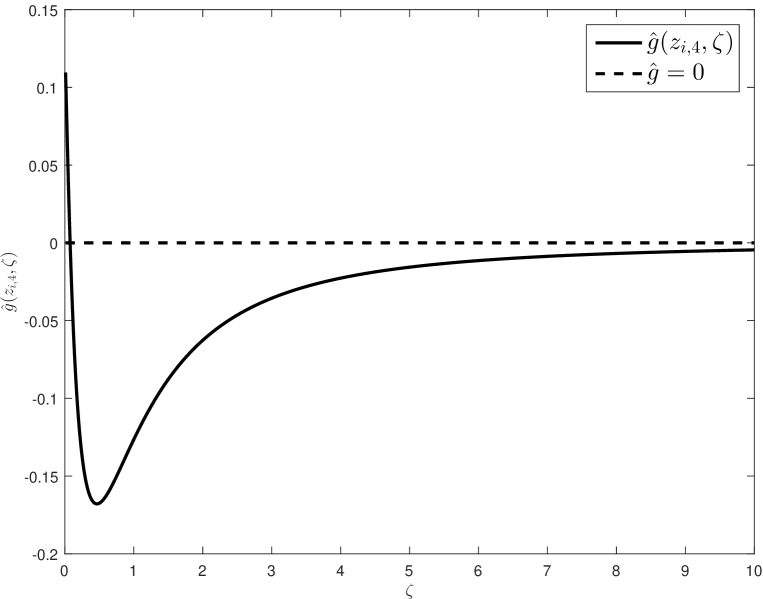
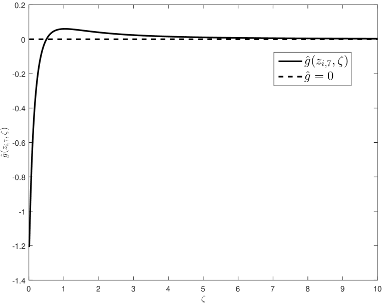
Figure D.1: Plots of $\hat{g}(z_{1,M};\zeta)$ in terms of $\zeta$ for $M=4$ and $7$ from the left to right.

D.7 Proof of Theorem 5.4

Proof

Because the matrix $\vec{D}_{M}$ in (4.14) at $\vec{W}_{M}=\vec{W}_{M}^{(0)}$ can be reformed as follows

$$\vec{D}_{M}=\begin{pmatrix}\vec{D}_{3\times 3}^{11}&\vec{D}_{3\times 2}^{12}&\vec{O}\\ \vec{O}&\vec{D}_{2\times 2}^{22}&\vec{O}\\ \vec{O}&\vec{O}&\vec{I}_{2M-4}\end{pmatrix},$$

and its inverse is given by

$$\vec{D}_{M}^{-1}=\begin{pmatrix}\left(\vec{D}_{3\times 3}^{11}\right)^{-1}&-\left(\vec{D}_{3\times 3}^{11}\right)^{-1}\vec{D}_{3\times 2}^{12}\left(\vec{D}_{2\times 2}^{22}\right)^{-1}&\vec{O}\\ \vec{O}&\left(\vec{D}_{2\times 2}^{22}\right)^{-1}&\vec{O}\\ \vec{O}&\vec{O}&\vec{I}_{2M-4}\end{pmatrix},$$

as well as

$$\tilde{\vec{D}}_{M}^{W}=\begin{pmatrix}\vec{O}&\vec{D}_{3\times 2}^{12}&\vec{O}\\ \vec{O}&\vec{D}_{2\times 2}^{22}&\vec{O}\\ \vec{O}&\vec{O}&\vec{I}_{2M-4}\end{pmatrix},$$

the product of $\tilde{\vec{D}}_{M}^{W}$ and $\vec{D}_{M}^{-1}$ is of the following form

$$\tilde{\vec{D}}_{M}^{W}\vec{D}_{M}^{-1}=\begin{pmatrix}\vec{O}_{3\times 3}&\vec{D}_{3\times 2}^{12}\left(\vec{D}_{2\times 2}^{22}\right)^{-1}&\vec{O}_{3\times(2M-4)}\\ \vec{O}_{2\times 3}&\vec{I}_{2}&\vec{O}_{2\times(2M-4)}\\ \vec{O}_{(2M-4)\times 3}&\vec{O}_{(2M-4)\times 2}&\vec{I}_{2M-4}\end{pmatrix},$$

where $\vec{D}_{3\times 3}^{11}$ is the $3\times 3$ subblock of $\vec{D}_{2}$ in the upper left corner, $\vec{D}_{3\times 2}^{12}$ denotes the $3\times 2$ subblock of $\vec{D}_{2}$ in the upper right corner, and $\vec{D}_{2\times 2}^{22}$ is $2\times 2$ subblock of $\vec{D}_{2}$ in the bottom right corner. It is obvious that each eigenvalue of $-\tilde{\vec{D}}_{M}^{W}\vec{D}_{M}^{-1}$ is non-positive, so does the matrix

$$\bar{\vec{Q}}_{M}:=-\frac{1}{\tau}\left(U^{0}\vec{M}_{M}^{t}-U^{1}\vec{M}_{M}^{x}\right)^{\frac{1}{2}}\tilde{\vec{D}}_{M}^{W}\vec{D}_{M}^{-1}\left(U^{0}\vec{M}_{M}^{t}-U^{1}\vec{M}_{M}^{x}\right)^{-\frac{1}{2}}.$$

The matrix $U^{0}\vec{M}_{M}^{t}-U^{1}\vec{M}_{M}^{x}$ can be written as follows

$$\begin{pmatrix}\vec{M}_{3\times 3}^{11}&\vec{M}_{3\times 2}^{12}&\vec{O}_{3,2M-4}\\ (\vec{M}_{3\times 2}^{12})^{T}&\vec{M}_{2\times 2}^{22}&\vec{M}_{2\times(2M-4)}^{23}\\ \vec{O}_{2M-4,3}&(\vec{M}_{2\times(2M-4)}^{23})^{T}&\vec{M}_{(2M-4)\times(2M-4)}^{33}\end{pmatrix},$$

where $\vec{M}_{3\times 3}^{11}$ is the $3\times 3$ subblock of $\vec{P}_{2}^{p}\vec{A}_{2}^{0}(\vec{P}_{2}^{p})^{T}$ in the upper left corner, $\vec{M}_{3\times 2}^{12}$ denotes the $3\times 2$ subblock of $\vec{P}_{2}^{p}\vec{A}_{2}^{0}(\vec{P}_{2}^{p})^{T}$ in the upper right corner, and $\vec{M}_{2\times 2}^{22}$ is $2\times 2$ subblock of $\vec{P}_{2}^{p}\vec{A}_{2}^{0}(\vec{P}_{2}^{p})^{T}$ in the bottom right corner, the rest subblocks form the $(2M-2)\times(2M-2)$ bottom right corner of $\vec{P}_{2}^{p}\vec{A}_{M}^{0}(\vec{P}_{M}^{p})^{T}$. Thus one has

$$\vec{M}_{D}:=(\vec{M}_{3\times 2}^{12})^{T}\vec{D}_{3\times 2}^{12}\left(\vec{D}_{2\times 2}^{22}\right)^{-1}=-\left(\vec{D}_{3\times 2}^{12}\left(\vec{D}_{2\times 2}^{22}\right)^{-1}\right)^{T}\vec{M}_{3\times 3}^{11}\left(\vec{D}_{3\times 2}^{12}\left(\vec{D}_{2\times 2}^{22}\right)^{-1}\right),$$

which is symmetric because $\vec{M}_{3\times 3}^{11}\vec{D}_{3\times 2}^{12}\left(\vec{D}_{2\times 2}^{22}\right)^{-1}+\vec{M}_{3\times 2}^{12}=\vec{O}_{3\times 2}.$

On the other hands, because the first three components of $\vec{S}(\vec{W}_{M})$ are zero, all elements in the first three rows and the first three columns of the matrix

$$\vec{Q}_{M}=-\frac{1}{\tau}\left(U^{0}\vec{M}_{M}^{t}-U^{1}\vec{M}_{M}^{x}\right)\tilde{\vec{D}}_{M}^{W}\vec{D}_{M}^{-1},$$

are zero, and the matrix $\vec{Q}_{M}$ is of form

$$\vec{Q}_{M}=-\frac{1}{\tau}\begin{pmatrix}\vec{O}_{3,3}&\vec{O}_{3,2}&\vec{O}_{3,2M-4}\\ \vec{O}_{2,3}&\vec{M}_{2\times 2}^{22}+\vec{M}_{D}&\vec{M}_{2\times(2M-4)}^{23}\\ \vec{O}_{2M-4,3}&(\vec{M}_{2\times(2M-4)}^{23})^{T}&\vec{M}_{(2M-4)\times(2M-4)}^{33}\end{pmatrix}.$$

Hence the matrix $\vec{Q}_{M}$ is symmetric. It is obvious that $\vec{Q}_{M}$ is congruent with $\bar{\vec{Q}}_{M}$, so it is negative semi-definite.

Because both matrices $\vec{D}_{M}$ and $\vec{M}_{M}^{t}$ are invertible, and $\vec{M}_{M}^{t}$ is positive definite, (5.4) is equivalent to

$$\det\left(i\omega\vec{I}-ik\vec{M}_{M}-\hat{\vec{Q}}_{M}\right)=0,$$ (D.2)

where

$$\hat{\vec{Q}}_{M}:= \left(\vec{M}_{M}^{t}\right)^{-\frac{1}{2}}\vec{Q}_{M}\left(\vec{M}_{M}^{t}\right)^{-\frac{1}{2}},$$

and

$$\vec{M}_{M}:=\left(\vec{M}_{M}^{t}\right)^{-\frac{1}{2}}\vec{M}_{M}^{x}\left(\vec{M}_{M}^{t}\right)^{-\frac{1}{2}}.$$

It is obvious that the matrix $\hat{\vec{Q}}_{M}$ is congruent with $\vec{Q}_{M}$ and negative semi-definite, and $\vec{M}_{M}$ is symmetric. Using Lemmas 1 and 2 in LS:2016 completes the proof. ∎

D.8 Proof of Lemma 10

Proof

• Under the given Lorentz boost ($x$ direction)

  $$t^{\prime}=\gamma(v)(t-vx),\ x^{\prime}=\gamma(v)(x-vt),\ \gamma(v)=(1-v^{2})^{-\frac{1}{2}},$$

  where $v$ is the relative velocity between frames in the $x$-direction, one has

  $$(p^{0})^{\prime}=\gamma(v)(p^{0}-p^{1}v),\quad(p^{1})^{\prime}=\gamma(v)(p^{1}-p^{0}v),$$

  $$(U^{0})^{\prime}=\gamma(v)(U^{0}-U^{1}v),\quad(U^{1})^{\prime}=\gamma(v)(U^{1}-U^{0}v).$$

  Thus one further obtains

  $$E^{\prime}=(U^{0})^{\prime}(p^{0})^{\prime}-(U^{1})^{\prime}(p^{1})^{\prime}=U^{0}p^{0}-U^{1}p^{1}=E,$$

  and

  $$\left(\frac{p_{<1>}}{U^{0}}\right)^{\prime}= \frac{-(p^{<1>})^{\prime}}{(U^{0})^{\prime}}=-\frac{p^{<0>}-p^{<1>}v}{U^{1}-U^{0}v}=-\frac{(U^{0})^{-1}U^{1}p^{<1>}-p^{<1>}v}{U^{1}-U^{0}v}=\frac{p_{<1>}}{U^{0}},$$

  $$\left(\frac{dp}{p^{0}}\right)^{\prime}= \frac{d(p^{1})^{\prime}}{(p^{0})^{\prime}}=\frac{dp^{0}-dp^{1}v}{p^{1}-p^{0}v}=\frac{(p^{0})^{-1}p^{1}dp^{1}-dp^{1}v}{p^{1}-p^{0}v}=\frac{dp}{p^{0}}.$$

  Combining them with (4.9) gives that each component of $\vec{f}_{M}$ is Lorentz invariant, such that the last $(2M-4)$ components of $\vec{W}_{M}$ are also Lorentz invariant.

  From (2.20), it is not difficult to prove that $\rho$ and $\theta$ are Lorentz invariant. On the other hand, because

  $$\tilde{n}^{1}=\int_{\mathbb{R}}\frac{p^{<1>}}{U^{0}}f\frac{dp}{p^{0}},$$

  the quantity $\tilde{n}^{1}$ is Lorentz invariant. Moreover, on has

  $$\left(\frac{du}{1-u^{2}}\right)^{\prime}=\frac{d(U^{1})^{\prime}}{(U^{0})^{\prime}}=\frac{dU^{0}-dU^{1}v}{U^{1}-U^{0}v}=\frac{(U^{0})^{-1}U^{1}dU^{1}-dU^{1}v}{U^{1}-U^{0}v}=\frac{dU^{1}}{U^{0}}=\frac{du}{1-u^{2}}.$$

  Using the above results completes the proof of the first part.

• Because $\vec{A}_{M}^{0}$ and $\vec{A}_{M}^{1}$ only depend on $\theta$, they are Lorentz invariant.

  The source term $\vec{S}(\vec{W}_{M})$ in (4.21) can be rewritten into

  $$\vec{S}(\vec{W}_{M})=-\frac{1}{\tau}\vec{P}_{M}^{p}\vec{A}_{M}^{0}(\vec{P}_{M}^{p})^{T}\left(\vec{f}_{M}-\vec{f}^{(0)}_{M}\right),$$

  which has been expressed in terms of the Lorentz covariant quantities. In fact, the general source term $\vec{S}(\vec{W}_{M})$ in the moment system (4.20) is also Lorentz invariant. The proof is completed.

∎

D.9 Proof of Theorem 5.5

Proof

From the 3rd step in Sec. 4.2 and Lemma 10, one knows that $\hat{\vec{D}}_{M}=\vec{D}_{M}(\vec{D}_{M}^{u})^{-1}$ can be expressed in terms of the Lorentz covariant quantities, so it is Lorentz invariant. Because

$$(\vec{M}_{M}^{t})^{\prime} =-\gamma(v)(U^{1}-U^{0}v)\vec{P}_{M}^{p}\vec{A}_{M}^{1}(\vec{P}_{M}^{p})^{T}+\gamma(v)(U^{0}-U^{1}v)\vec{P}_{M}^{p}\vec{A}_{M}^{0}(\vec{P}_{M}^{p})^{T},$$

$$(\vec{M}_{M}^{x})^{\prime} =-\gamma(v)(U^{0}-U^{1}v)\vec{P}_{M}^{p}\vec{A}_{M}^{1}(\vec{P}_{M}^{p})^{T}+\gamma(v)(U^{1}-U^{0}v)\vec{P}_{M}^{p}\vec{A}_{M}^{0}(\vec{P}_{M}^{p})^{T},$$

and

$$\left(\frac{\partial}{\partial t}\right)^{\prime}=\gamma(v)\left(\frac{\partial}{\partial t}+v\frac{\partial}{\partial x}\right),\quad\left(\frac{\partial}{\partial x}\right)^{\prime}=\gamma(v)\left(\frac{\partial}{\partial x}+v\frac{\partial}{\partial t}\right),$$

one has

$$\left(\vec{D}_{M}^{u}\frac{\partial\vec{W}_{M}}{\partial t}\right)^{\prime}= {\rm diag}\left\{1,\big{(}(U^{0})^{2}\big{)}^{\prime},1,\cdots,1\right\}\gamma(v)\left(\frac{\partial(\rho,u^{\prime},\theta,\Pi,\tilde{n}^{1},f_{3}^{0},\cdots,f_{M-1}^{1})^{T}}{\partial t}\right.$$

$$+\left.v\frac{\partial(\rho,u^{\prime},\theta,\Pi,\tilde{n}^{1},f_{3}^{0},\cdots,f_{M-1}^{1})^{T}}{\partial x}\right)$$

$$= {\rm diag}\left\{1,\big{(}(U^{0}\big{)}^{-1})^{\prime},1,\cdots,1\right\}\gamma(v)\left(\frac{\partial(\rho,(U^{1})^{\prime},\theta,\Pi,\tilde{n}^{1},f_{3}^{0},\cdots,f_{M-1}^{1})^{T}}{\partial t}\right.$$

$$+\left.v\frac{\partial(\rho,(U^{1})^{\prime},\theta,\Pi,\tilde{n}^{1},f_{3}^{0},\cdots,f_{M-1}^{1})^{T}}{\partial x}\right)$$

$$= \vec{D}_{M}^{u}\gamma(v)\left(\frac{\partial\vec{W}_{M}}{\partial t}+v\frac{\partial\vec{W}_{M}}{\partial x}\right),$$

where the last equal sign is derived by following the proof of Lemma 10. Similarly, one has

$$\left(\vec{D}_{M}^{u}\frac{\partial\vec{W}_{M}}{\partial x}\right)^{\prime}=\vec{D}_{M}^{u}\gamma(v)\left(\frac{\partial\vec{W}_{M}}{\partial x}+v\frac{\partial\vec{W}_{M}}{\partial t}\right).$$

Thus one obtains

$$\left(\vec{B}_{M}^{0}\frac{\partial\vec{W}_{M}}{\partial t}+\vec{B}_{M}^{1}\frac{\partial\vec{W}_{M}}{\partial x}\right)^{\prime}$$

$$= (\vec{M}_{M}^{t})^{\prime}\left(\vec{D}_{M}\frac{\partial\vec{W}_{M}}{\partial t}\right)^{\prime}+(\vec{M}_{M}^{x})^{\prime}\left(\vec{D}_{M}\frac{\partial\vec{W}_{M}}{\partial x}\right)^{\prime}$$

$$= \left(-(U^{1})^{\prime}\vec{P}_{M}^{p}\vec{A}_{M}^{1}(\vec{P}_{M}^{p})^{T}+(U^{0})^{\prime}P_{M}^{p}\vec{A}_{M}^{0}(P_{M}^{p})^{T}\right)\vec{D}_{M}\left(\gamma(v)\left(\frac{\partial\vec{W}_{M}}{\partial t}+v\frac{\partial\vec{W}_{M}}{\partial x}\right)\right)$$

$$+\left(-(U^{0})^{\prime}\vec{P}_{M}^{p}\vec{A}_{M}^{1}(\vec{P}_{M}^{p})^{T}+(U^{1})^{\prime}\vec{P}_{M}^{p}\vec{A}_{M}^{0}(\vec{P}_{M}^{p})^{T}\right)\vec{D}_{M}\left(\gamma(v)\left(\frac{\partial\vec{W}_{M}}{\partial x}+v\frac{\partial\vec{W}_{M}}{\partial t}\right)\right)$$

$$= \left(-U^{1}v\vec{P}_{M}^{p}\vec{A}_{M}^{1}(\vec{P}_{M}^{p})^{T}+U^{0}\vec{P}_{M}^{p}\vec{A}_{M}^{0}(\vec{P}_{M}^{p})^{T}\right)\vec{D}_{M}\frac{\partial\vec{W}_{M}}{\partial t}$$

$$+\left(-U^{0}\vec{P}_{M}^{p}\vec{A}_{M}^{1}(\vec{P}_{M}^{p})^{T}+U^{1}\vec{P}_{M}^{p}\vec{A}_{M}^{0}(\vec{P}_{M}^{p})^{T}\right)\vec{D}_{M}\frac{\partial\vec{W}_{M}}{\partial x}$$

$$= \vec{B}_{M}^{0}\frac{\partial\vec{W}_{M}}{\partial t}+\vec{B}_{M}^{1}\frac{\partial\vec{W}_{M}}{\partial x}.$$

Combining it with Lemma 10 completes the proof. ∎

Appendix E Proofs in Section 6

E.1 Proof of Lemma 11

Proof

Using Lemmas 4 and 7 gives

$$\tilde{f}g^{(0)}_{[u,\theta]}= \sum_{i=0}^{M}\tilde{f}_{i}^{0}\tilde{P}_{i}^{(0)}[u,\theta]+\sum_{j=0}^{M-1}\tilde{f}_{j}^{1}\tilde{P}_{j}^{(1)}[u,\theta],$$

$$\Pi_{M}[u,\theta]f= \sum_{i=0}^{M}f_{i}^{0}\tilde{P}_{i}^{(0)}[u,\theta]+\sum_{j=0}^{M-1}f_{j}^{(1)}\tilde{P}_{j}^{(1)}[u,\theta],$$

where

$$f_{i}^{0} =<f,\tilde{P}_{i}^{(0)}[u,\theta]>_{g^{(0)}_{[u,\theta]}},\quad\tilde{f}_{i}^{0}=<\tilde{f}g^{(0)}_{[u,\theta]},\tilde{P}_{i}^{(0)}[u,\theta]>_{g^{(0)}_{[u,\theta]}},\quad i\leq M,$$

$$f_{j}^{1} =<f,\tilde{P}_{j}^{(1)}[u,\theta]>_{g^{(0)}_{[u,\theta]}},\quad\tilde{f}_{j}^{1}=<\tilde{f}g^{(0)}_{[u,\theta]},\tilde{P}_{j}^{(1)}[u,\theta]>_{g^{(0)}_{[u,\theta]}},\quad j\leq M-1.$$

Therefore one has

$$<\tilde{f}g^{(0)}_{[u,\theta]},\Pi_{M}[u,\theta]f>_{g^{(0)}_{[u,\theta]}}=<\tilde{f}f,\Pi_{M}[u,\theta]f>_{f}$$

$$= \sum_{i=0}^{M}f_{i}^{0}<\tilde{f}f,\tilde{P}_{i}^{(0)}[u,\theta]>_{f}+\sum_{j=0}^{M-1}f_{j}^{1}<\tilde{f}f,\tilde{P}_{j}^{(1)}[u,\theta]>_{f}$$

$$= \sum_{i=0}^{M}f_{i}^{0}<\tilde{f}g^{(0)}_{[u,\theta]},\tilde{P}_{i}^{(0)}[u,\theta]>_{g^{(0)}_{[u,\theta]}}+\sum_{j=0}^{M-1}f_{j}^{1}<\tilde{f}g^{(0)}_{[u,\theta]},\tilde{P}_{j}^{(1)}[u,\theta]>_{g^{(0)}_{[u,\theta]}}$$

$$= \sum_{i=0}^{M}f_{i}^{0}\tilde{f}_{i}^{0}+\sum_{j=0}^{M-1}f_{j}^{1}\tilde{f}_{j}^{1}$$

$$= \sum_{i=0}^{M}<f,\tilde{f}_{i}^{0}\tilde{P}_{i}^{(0)}[u,\theta]>_{g^{(0)}_{[u,\theta]}}+\sum_{j=0}^{M-1}<f,\tilde{f}_{j}^{1}\tilde{P}_{j}^{(1)}[u,\theta]>_{g^{(0)}_{[u,\theta]}}$$

$$= <f,\tilde{f}g^{(0)}_{[u,\theta]}>_{g^{(0)}_{[u,\theta]}}=<f,\tilde{f}f>_{f}.$$

The proof is completed. ∎

E.2 Proof of Lemma 12

Proof

Using Lemma 7 gives

$$\Pi_{M}[u_{1},\theta_{1}]f=\sum_{i=0}^{M}f_{i}^{0}\tilde{P}_{i}^{(0)}[u_{1},\theta_{1}]+\sum_{j=0}^{M-1}f_{j}^{1}\tilde{P}_{i}^{(1)}[u_{1},\theta_{1}],$$

$$\Pi_{M}[u_{1},\theta_{1}]\Pi_{M}[u_{2},\theta_{2}]f=\sum_{i=0}^{M}\tilde{f}_{i}^{0}\tilde{P}_{i}^{(0)}[u_{1},\theta_{1}]+\sum_{j=0}^{M-1}\tilde{f}_{j}^{1}\tilde{P}_{j}^{(1)}[u_{1},\theta_{1}],$$

$$f_{i}^{0} =<f,\tilde{P}_{i}^{(0)}[u_{1},\theta_{1}]>_{g^{(0)}_{[u_{1},\theta_{1}]}}={<f,{P}_{i}^{(0)}(u_{1},\zeta_{1})f>_{f}},i\leq M,$$

$$f_{j}^{1} =<f,\tilde{P}_{j}^{(1)}[u_{1},\theta_{1}]>_{g^{(0)}_{[u_{1},\theta_{1}]}}={<f,{P}_{j}^{(1)}(u_{1},\zeta_{1})(U_{0})_{1}^{-1}p_{<1>}f>_{f}},j\leq M-1,$$

$$\tilde{f}_{i}^{0} =<\Pi_{M}[u_{2},\theta_{2}]f,\tilde{P}_{i}^{(0)}[u_{1},\theta_{1}]>_{g^{(0)}_{[u_{1},\theta_{1}]}}={<\Pi_{M}[u_{2},\theta_{2}]f,{P}_{i}^{(0)}(u_{1},\zeta_{1})f>_{f}},i\leq M,$$

$$\tilde{f}_{j}^{1} =<\Pi_{M}[u_{2},\theta_{2}]f,\tilde{P}_{j}^{(1)}[u_{1},\theta_{1}]>_{g^{(0)}_{[u_{1},\theta_{1}]}}={<\Pi_{M}[u_{2},\theta_{2}]f,{P}_{j}^{(1)}(u_{1},\zeta_{1})(U_{0})_{1}^{-1}p_{<1>}f>_{f}},j\leq M-1,$$

Because both ${P}_{i}^{(0)}(u_{1},\zeta_{1})f$ and ${P}_{j}^{(1)}(u_{1},\zeta_{1})(U_{0})_{1}^{-1}p_{<1>}f$ belong to the space $\mathbb{H}_{M}^{f}$, using Lemma 11 completes the proof. ∎

E.3 Proof of Theorem 6.1

Proof

Because Eq. (6.3) is equivalent to

$$\left(\vec{I}+\frac{\Delta t}{\tau_{i}^{\ast}}\left(\vec{M}_{i,M}^{t\ast}\right)^{-1}\left(U_{i}^{0\ast}\vec{M}_{i,M}^{t\ast}-U_{i}^{1\ast}\vec{M}_{i,M}^{x\ast}\right)\left(\vec{I}-\vec{D}_{i,M}^{f_{i}^{(0)\ast}}\right)\right)\vec{f}_{i,M}^{n+1}=\vec{f}_{i,M}^{\ast},$$

it is unconditionally stable if and only if the modulus of each eigenvalue of the matrix

$$\vec{I}+\frac{\Delta t}{\tau_{i}^{\ast}}\left(\vec{M}_{i,M}^{t\ast}\right)^{-1}\left(U_{i}^{0\ast}\vec{M}_{i,M}^{t\ast}-U_{i}^{1\ast}\vec{M}_{i,M}^{x\ast}\right)\left(\vec{I}-\vec{D}_{i,M}^{f_{i}^{(0)\ast}}\right),$$

is not less than one. It is true if the real part of each eigenvalue of the matrix

$$\left(\vec{M}_{i,M}^{t\ast}\right)^{-1}\left(U_{i}^{0\ast}\vec{M}_{i,M}^{t\ast}-U_{i}^{1\ast}\vec{M}_{i,M}^{x\ast}\right)\left(\vec{I}-\vec{D}_{i,M}^{f_{i}^{(0)\ast}}\right)=:\left(\vec{M}_{i,M}^{t\ast}\right)^{-1}\bar{\vec{M}}_{D}^{*},$$ (E.1)

is non-negative.

In fact, thanks to (6.4), the characteristic polynomial of the upper triangular matrix $\vec{I}-\vec{D}_{i,M}^{f_{i}^{(0)\ast}}$ is explicitly given by

$$0=\det\left(\lambda\vec{I}-\left(\vec{I}-\vec{D}_{i,M}^{f_{i}^{(0)\ast}}\right)\right)=\det\left((\lambda-1)\vec{I}+\vec{D}_{i,M}^{f^{(0)\ast}}\right)=\lambda(\lambda-1)^{2M},$$

and $\bar{\vec{M}}_{D}^{*}$ is a symmetric matrix and congruent with

$$\left(U_{i}^{0\ast}\vec{M}_{i,M}^{t\ast}-U_{i}^{1\ast}\vec{M}_{i,M}^{x\ast}\right)^{\frac{1}{2}}\left(\vec{I}-\vec{D}_{i,M}^{f_{i}^{(0)\ast}}\right)\left(U_{i}^{0\ast}\vec{M}_{i,M}^{t\ast}-U_{i}^{1\ast}\vec{M}_{i,M}^{x\ast}\right)^{-\frac{1}{2}},$$

which is similar to the matrix $\vec{I}-\vec{D}_{i,M}^{f_{i}^{(0)\ast}}$. Thus the matrix $\bar{\vec{M}}_{D}^{*}$ is positive semi-definite and each eigenvalue of the matrix $\left(\vec{M}_{i,M}^{t\ast}\right)^{-1}\bar{\vec{M}}_{D}^{\ast}$ is non-negative because of the relation $\left(\vec{M}_{i,M}^{t\ast}\right)^{-1}\bar{\vec{M}}_{D}^{\ast}=\left(\vec{M}_{i,M}^{t\ast}\right)^{-\frac{1}{2}}\big{(}\left(\vec{M}_{i,M}^{t\ast}\right)^{-\frac{1}{2}}\bar{\vec{M}}_{D}^{\ast}\left(\vec{M}_{i,M}^{t\ast}\right)^{-\frac{1}{2}}\big{)}\left(\vec{M}_{i,M}^{t\ast}\right)^{\frac{1}{2}}$ . The proof is completed. ∎

References

- (1) J.L. Anderson, Relativistic Boltzmann theory and Grad method of moments, in Relativity, edited by M. Carmeli, S.I. Fickler, and L. Witten, Springer, 109-124, 1970.
- (2) J.L. Anderson, Relativistic Grad polynomials, J. Math. Phys., 15, 1116-1119, 1974.
- (3) J.L. Anderson and H.R. Witting, A relativistic relaxation-time model for the Boltzmann equation, Physica, 74, 466-488, 1974.
- (4) J.D. Au, M. Torrilhon, and W. Weiss, The shock tube study in extended thermodynamics, Phys. Fluids, 13, 2423-2432, 2001.
- (5) Z. Cai, Y. Fan, and R. Li, Globally hyperbolic regularization of Grad’s moment system in one dimensional space, Commun. Math. Sci., 11, 547-571, 2013.
- (6) Z. Cai, Y. Fan, and R. Li, Globally hyperbolic regularization of Grad’s moment system, Comm. Pure Appl. Math., 67, 464-518, 2014.
- (7) Z. Cai, Y. Fan, and R. Li, On hyperbolicity of 13-moment system, Kinet. Relat. Mod., 7, 415-432, 2014.
- (8) Z. Cai, Y. Fan, and R. Li, A framework on moment model reduction for kinetic equation, SIAM J. Appl. Math., 75, 2001-2023, 2014.
- (9) Z. Cai and R. Li, Numerical regularized moment method of arbitrary order for Boltzmann-BGK equation, SIAM J. Sci. Comput., 32, 2875-2907, 2010.
- (10) Z. Cai, R. Li, and Y. Wang, Numerical regularized moment method for high Mach number flow, Commun. Comput. Phys., 11, 1415-1438, 2012.
- (11) C. Cercignani, The Boltzmann Equation and Its Applications, Springer, 1988.
- (12) C. Cercignani and G.M. Kremer, The Relativistic Boltzmann Equation: Theory and Applications, Birkhauser, 2002.
- (13) S. Chapman and T.G. Cowling, The Mathematical Theory of Non-uniform Gases, 3rd ed., Cambridge Univ. Press, 1991.
- (14) G.S. Denicol, H. Niemi, E. Molnár, and D.H. Rischke, Derivation of transient relativistic fluid dynamics from the Boltzmann equation, Phys. Rev. D, 85, 114047, 2012.
- (15) G.S. Denicol, T. Kodama, T. Koide, and Ph. Mota, Stability and causality in relativistic dissipative hydrodynamics, J. Phys. G: Nucl. Part. Phys., 35, 115102, 2008.
- (16) Y. Di, Y. Fan, R. Li, and L. Zheng, Linear stability of hyperbolic moment models for Boltzmann equation, arXiv:1609.03669, 2016.
- (17) C. Eckart, The thermodynamics of irreversible processes. III. Relativistic theory of the simple fluid, Phys. Rev., 58, 919-924, 1940.
- (18) A. Einstein, Relativity: The Special and the General Theory, Three Rivers Press, 1995.
- (19) Y. Fan, J. Koellermeier, J. Li, R. Li, and M. Torrilhon, Model reduction of kinetic equations by operator projection, J. Stat. Phys., 162, 457-486, 2016.
- (20) W. Florkowski, A. Jaiswal, E. Maksymiuk, R. Ryblewski, and M. Strickland, Relativistic quantum transport coefficients for second-order viscous hydrodynamics, Phys. Rev. C, 91, 054907, 2015.
- (21) A.L. Garcia-Perciante, A. Sandoval-Villalbazob, L.S. Garcia-Colin, Generalized relativistic Chapman-Enskog solution of the Boltzmann equation, Physica A, 21, 5073-5079, 2008.
- (22) H. Grad, On the kinetic theory of rarefied gases, Commun. Pure Appl. Math., 2, 331-407, 1949.
- (23) H. Grad, Note on -dimensional Hermite polynomials, Commun. Pure Appl. Math., 2, 325-330 1949.
- (24) S.R.D. Groot, W.A.V. Leeuwen, and C.G.V. Weert, Relativistic Kinetic Theory: Principles and Applications, North-Holland Press, 1980.
- (25) W.A. Hiscock and L. Lindblom, Stability and causality in dissipative relativistic fluids, Ann. Phys., 151, 466-496, 1983.
- (26) W.A. Hiscock and L. Lindblom, Generic instabilities in first-order dissipative relativistic fluid theories, Phys. Rev. D, 31, 725-733, 1985.
- (27) W.A. Hiscock and L. Lindblom, Linear plane waves in dissipative relativistic fluids, Phys. Rev. D, 35, 3723-3732, 1987.
- (28) W.A. Hiscock and L. Lindblom, Nonlinear pathologies in relativistic heat-conducting fluid theories, Phys. Lett. A, 131, 509-513, 1988.
- (29) W.A. Hiscock and T.S. Olson, Effects of frame choice on nonlinear dynamics in relativistic heat-conducting fluid theories, Phys. Lett. A, 141, 125-130, 1989.
- (30) W. Israel, Relativistic kinetic theory of a simple gas, J. Math. Phys., 4, 1163-1181, 1963.
- (31) W. Israel and J.M. Stewart, Thermodynamics of nonstationary and transient effects in a relativistic gas, Phys. Lett. A, 58, 213-215, 1976.
- (32) W. Israel and J.M. Stewart, Transient relativistic thermodynamics and kinetic theory, Ann. Phys., 118, 341-372 , 1979.
- (33) W. Israel and J.M. Stewart, On transient relativistic thermodynamics and kinetic theory II, Proc. R. Soc. Lond. A, 365, 43-52, 1979.
- (34) A. Jaiswal, Relativistic third-order dissipative fluid dynamics from kinetic theory, Phys. Rev. C, 88, 021903(R), 2013.
- (35) F. Jüttner, Das Maxwellsche gesetz der geschwindigkeitsverteilung in der relativtheorie, Ann. Physik und Chemie, 339, 856-882, 1911.
- (36) J. Koellermeier and M. Torrilhon, Hyperbolic moment equations using quadrature based projection methods, AIP Conf. Proc., 1628, 626-633, 2014.
- (37) J. Koellermeier, R. Schaerer, and M. Torrilhon, A framework for hyperbolic approximation of kinetic equations using quadrature-based projection methods, Kinet. Relat. Mod., 7, 531-549, 2014.
- (38) M. Kranyš, Kinetic derivation of nonstationary general relativistic thermodynamics, Nuovo Cim., 8B, 417-441, 1972.
- (39) L.D. Landau and E.M. Lifshitz, Fluid Mechanics, 2nd ed., Pergamon Press, 1987.
- (40) A. Lichnerowicz and R. Marrot, Propriétés statistiques des ensembles de particules en relativité restreite, C. R. Acad. Sci. Paris, 210, 759-761, 1940.
- (41) C. Marle, Modèle cinétique pour l’établissement des lois de la conduction de la chaleur et de la viscosité en theorié de la relativité, C.R. Acad. Sc. Paris., 260, 6539-6541, 1965.
- (42) L. Mieussens, Discrete velocity model and implicit scheme for the BGK equation of rarefied gas dynamics, Math. Models Methods Appl. Sci., 10, 1121-1149, 2000.
- (43) I. Müller and T. Ruggeri, Rational Extended Thermodynamics, 2nd ed., Springer-Verlag, 1998.
- (44) S. Rhebergen, O. Bokhove, and J.J.W. van der Vegt, Discontinuous Galerkin finite element methods for hyperbolic nonconservative partial differential equations, J. Comput. Phys., 227, 1887-1922, 2008.
- (45) J. Shen, T. Tang, and L. Wang, Spectral Methods: Algorithms, Analysis and Applications, Springer, 2011.
- (46) J.M. Stewart, On transient relativistic thermodynamics and kinetic theory, Proc. R. Soc. Lond. A, 357, 59-75, 1977.
- (47) H. Struchtrup, Projected moments in relativistic kinetic theory, Physica A, 253, 555-593, 1998.