Representing convex geometries by almost-circles

Abstract.

Finite convex geometries are combinatorial structures. It follows from a recent result of M. Richter and L.G. Rogers that there is an infinite set $T_{\textup{RR}}$ of planar convex polygons such that $T_{\textup{RR}}$ with respect to geometric convex hulls is a locally convex geometry and every finite convex geometry can be represented by restricting the structure of $T_{\textup{RR}}$ to a finite subset in a natural way. An almost-circle of accuracy $1-\epsilon$ is a differentiable convex simple closed curve $S$ in the plane having an inscribed circle of radius $r_{1}>0$ and a circumscribed circle of radius $r_{2}$ such that the ratio $r_{1}/r_{2}$ is at least $1-\epsilon$. Motivated by Richter and Rogers’ result, we construct a set $T_{\textup{new}}$ such that (1) $T_{\textup{new}}$ contains all points of the plane as degenerate singleton circles and all of its non-singleton members are differentiable convex simple closed planar curves; (2) $T_{\textup{new}}$ with respect to the geometric convex hull operator is a locally convex geometry; (3) as opposed to $T_{\textup{RR}}$, $T_{\textup{new}}$ is closed with respect to non-degenerate affine transformations; and (4) for every (small) positive $\epsilon\in\mathbb{R}$ and for every finite convex geometry, there are continuum many pairwise affine-disjoint finite subsets $E$ of $T_{\textup{new}}$ such that each $E$ consists of almost-circles of accuracy $1-\epsilon$ and the convex geometry in question is represented by restricting the convex hull operator to $E$. The affine-disjointness of $E_{1}$ and $E_{2}$ means that, in addition to $E_{1}\cap E_{2}=\emptyset$, even $\psi(E_{1})$ is disjoint from $E_{2}$ for every non-degenerate affine transformation $\psi$.

1. Introduction

For a set $E$, let $\textup{Pow}(E)=\{X:X\subseteq E\}$ and $\operatorname{\textup{Pow}_{\textup{fin}}}(E)=\{X:X\subseteq E$ and $X$ is finite$\}$ denote the powerset and the set of finite subsets of $E$, respectively. Convex geometries are defined as follows.

Definition 1.1 (Adaricheva and Nation [2] and [3]).

A pair $\langle E;\Phi\rangle$ is a convex geometry, also called an anti-exchange system, if it satisfies the following properties:

1. $E$ is a set, called the set of points, and $\Phi\colon\textup{Pow}(E)\to\textup{Pow}(E)$ is a closure operator, that is, for all $X\subseteq Y\subseteq E$, we have $X\subseteq\Phi(X)\subseteq\Phi(Y)=\Phi(\Phi(Y))$.

2. If $A\in\textup{Pow}(E)$, $x,y\in E\setminus\Phi(A)$, and $\Phi(A\cup\{x\})=\Phi(A\cup\{y\})$, then $x=y$. (This is the so-called anti-exchange property.)

3. $\Phi(\emptyset)=\emptyset$.

Although local convexity is a known concept for topological vector spaces, the following concept seems to be new.

Definition 1.2.

A pair $\langle E;\Phi\rangle$ is a locally convex geometry if 1.1(i), 1.1(iii), and

1. If $X\in\operatorname{\textup{Pow}_{\textup{fin}}}(E)$, $d,d^{\prime}\in E\setminus\Phi(X)$, and $\Phi(X\cup\{d\})=\Phi(X\cup\{d^{\prime}\})$, then $d=d^{\prime}$.

(This condition will be called the local anti-exchange property.)

For example, if $\textup{Conv}_{\mathbb{R}^{n}}$ denotes the usual convex hull operator in the space $\mathbb{R}^{n}$,

(1.1) then $$\langle\mathbb{R}^{n};\textup{Conv}_{\mathbb{R}^{n}}\rangle$$ is a convex geometry.

Every convex geometry is a locally convex geometry but (1.4) we will soon show that the converse implication fails. Given a convex or a locally convex geometry $\langle E;\Phi\rangle$ and a subset $E_{0}$ of $E$, we can consider the restriction

(1.2) $${\langle E;\Phi\rangle}\kern-1.0pt\rceil_{\kern-1.0ptE_{0}}:=\langle E_{0};\Phi_{0}\rangle \Phi_{0}\colon\textup{Pow}(E_{0})\to\textup{Pow}(E_{0}) \Phi_{0}(X):=E_{0}\cap\Phi(X)$$, where the map is defined by the rule ,

of the original convex geometry to its subset, $E_{0}$. This terminology is justified by the following statement; without the trivial modification of adding “locally”, it is taken from Edelman and Jamison [12, Thm. 5.9].

Lemma 1.3 (Edelman and Jamison [12, Thm. 5.9]).

If $\langle E;\Phi\rangle$ is a convex or locally convex geometry, then so is its restriction ${\langle E;\Phi\rangle}\kern-1.0pt\rceil_{\kern-1.0ptE_{0}}$, for every subset $E_{0}$ of $E$.

Since our setting is slightly different and the proof is very short, we will prove this lemma in Section 3 for the reader’s convenience. Note that a finite locally convex geometry is automatically a convex geometry. As an additional justification of our terminology, we mention the following statement even if its proof, postponed to Section 3, is trivial.

Lemma 1.4.

A pair $\langle E;\Phi\rangle$ of a set $E$ and a closure operator $\Phi\colon\textup{Pow}(E)\to\textup{Pow}(E)$ on $E$ is a locally convex geometry if and only if its restriction ${\langle E;\Phi\rangle}\kern-1.0pt\rceil_{\kern-1.0ptE_{0}}$ is a convex geometry for every finite subset $E_{0}$ of $E$.

Finite convex geometries are intensively studied mathematical objects. There are several combinatorial and lattice theoretical ways to characterize and describe these objects; see, for example, Adaricheva and Czédli [1], Avann [4], Czédli [5], Dilworth [10], Duquenne [11], Edelman and Jamison [12], and see also Adaricheva and Nation [2] and Monjardet [14] for surveys. Natural and easy-to-visualize examples for finite convex geometries are obtained by considering the restrictions ${\langle\mathbb{R}^{n};\textup{Conv}_{\mathbb{R}^{n}}\rangle}\kern-1.0pt\rceil_{\kern-1.0ptE}$ of $\langle\mathbb{R}^{n};\textup{Conv}_{\mathbb{R}^{n}}\rangle$ to finite sets $E\subseteq\mathbb{R}^{n}$ of points, for $n\in\{1,2,3,\dots\}$. Note that most of the finite convex geometries are not isomorphic to any of these restrictions. The first result that represents every finite convex geometry with the help of $\langle\mathbb{R}^{n};\textup{Conv}_{\mathbb{R}^{n}}\rangle$ was proved in Kashiwabara, Nakamura, and Okamoto [13]. This result uses auxiliary points and has not much to do with restrictions in our sense, so we do not give further details on it.

Next, let $T$ be a set of subsets of the plane. For $X\subseteq T$, we can naturally define

(1.3) $$\textup{Points}(X) =\bigcup_{C\in X}C,\quad\text{ and}$$

$$\textup{Conv}_{T}(X): =\{D\in T:D\subseteq\textup{Conv}_{\mathbb{R}^{2}}(\textup{Points}(X))\}.$$

The notation Points is self-explanatory; $\textup{Points}(X)$ is the set of points of the members of $X$. Note the difference between the notations $\textup{Conv}_{\mathbb{R}^{2}}$ and $\textup{Conv}_{T}$; the former applies to sets of points and yields a set of points while the latter to sets of sets and yields a set of sets. Typically in the present paper, $T$ consists of closed curves and we apply $\textup{Conv}_{T}$ to sets of closed curves.

In lucky cases but far from always, the structure $\langle T;\textup{Conv}_{T}\rangle$ is a locally convex geometry. For example, if $T=\mathbb{R}^{2}$, then $\langle T;\textup{Conv}_{T}\rangle=\langle\mathbb{R}^{2};\textup{Conv}_{\mathbb{R}^{2}}\rangle$ is even a convex geometry. In order to obtain a more interesting example, let $T_{\textup{ellipses}}$ be the set of all non-flat ellipses in the plane. Here, by a non-flat ellipse we mean an ellipse that is either of positive area or it consists of a single point. We have the following observation.

(1.4) $$\langle T_{\textup{ellipses}};\textup{Conv}_{T_{\textup{ellipses}}}\rangle$$ is a locally convex geometry. However, it is not a convex geometry.

The first part of (1.4) follows from Czédli [6], where the argument is formulated only for circles but it clearly holds for ellipses. This part will also follow easily from the present paper; see the proof of part (ii) of Theorem 1.8. In order to see the second part, let $\mathbb{Z}$ stand for the set of integer numbers, and let $C_{k}=\{\langle x,y\rangle:(x-k)^{2}+y^{2}=1\}$, $X=\{\langle x,y\rangle:x^{2}+(y-3)^{2}=1\}$, and $Y=\{\langle x,y\rangle:x^{2}+(y-2)^{2}=4\}$. Then the anti-exchange property, 1.1(ii), fails for $A=\{C_{k}:k\in\mathbb{Z}\}$, $X$, and $Y$.

Related to [6, (4.6)], it is an open problem

(1.5) whether every finite convex geometry can be represented in the form $${\langle T_{\textup{ellipses}};\textup{Conv}_{T_{\textup{ellipses}}}\rangle}\kern-1.0pt\rceil_{\kern-1.0ptE}$$;

up to isomorphism, of course. The answer is affirmative for finite convex geometries of convex dimension at most 2, to be defined later; the reason is that, denoting the set of all circles (including the singletons) of the plane by $T_{\textup{circles}}$, [6] proves that

(1.6) every finite convex geometry of convex dimension at most $$2 {\langle T_{\textup{circles}};\textup{Conv}_{T_{\textup{circles}}}\rangle}\kern-1.0pt\rceil_{\kern-1.0ptE}$$ is isomorphic to some .

Actually, [6] proves a bit more but the details are irrelevant here.

We obtain from Richter and Rogers [15, Lemma 3], or in a straightforward way, that for every set $T$ of pairwise vertex-disjoint planar convex polygons, $\langle T;\textup{Conv}_{T}\rangle$ is a locally convex geometry. Therefore, since there are only countably many isomorphism classes of finite convex geometries, [15, Theorem] implies that

(1.7) there exists a set $$T_{\textup{RR}} \langle T_{\textup{RR}};\textup{Conv}_{T_{\textup{RR}}}\rangle {\langle T_{\textup{RR}};\textup{Conv}_{T_{\textup{RR}}}\rangle}\kern-1.0pt\rceil_{\kern-1.0ptE}$$ of pairwise vertex-disjoint convex polygons in the plane such that is a locally convex geometry and every finite convex geometry can be represented as some of its restrictions, .

Remark 1.5.

In this paper, the “elements” of our convex geometries are closed lines, mostly simple closed curves; for example, they are circles in (1.6). This setting is more natural here, since we will work with curves. However, it would be an equivalent setting to replace these “elements” by their convex hulls. For example, we could consider closed disks in (1.6) instead of circles, and similarly in (1.5), (1.7), and the forthcoming Theorem 1.8. However, instead of doing so, we require only that our simple closed curves should be convex, that is, they should coincide with the boundaries of their convex hulls.

Every non-degenerate affine transformation $\psi$ of the plane, that is, every map $\psi\colon\mathbb{R}^{2}\to\mathbb{R}^{2}$ defined by $\langle x,y\rangle\mapsto\langle x,y\rangle A+\langle b_{1},b_{2}\rangle$, where $A$ is a 2-by-2 matrix with nonzero determinant, is known to induce an automorphism of the convex geometry $\langle\mathbb{R}^{2};\textup{Conv}_{\mathbb{R}^{2}}\rangle$. Furthermore, if convex linear combinations are considered operations, then there are no more automorphisms, say, by Czédli, Maróti, and Romanowska [9, Theorem 2.4]. Hence and because of Remark 1.5, it is a natural desire to replace $T_{\textup{RR}}$ in (1.7) by a set of convex simple closed planar curves that is closed with respect to non-degenerate affine transformations. Note that $T_{\textup{RR}}$ is not even closed with respect to parallel shifts. Actually, except from trivial cases, if $T$ is a set of polygons closed with respect to parallel shifts, then $\langle T,\textup{Conv}_{T}\rangle$ is not a locally convex geometry in general; see Figure 1 for an explanation.

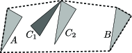
Figure 1. $\textup{Conv}_{T}(\{A,B\}\cup\{C_{1}\})=\textup{Conv}_{T}(\{A,B\}\cup\{C_{2}\})$, $\{C_{1},C_{2}\}\cap\textup{Conv}_{T}(\{A,B\})=\emptyset$, but $C_{1}\neq C_{2}$.

Our goal is to replace $T_{\textup{RR}}$ in (1.7) with a set of differentiable convex simple closed planar curves that is closed with respect to non-degenerate affine transformations. Although $T_{\textup{ellipses}}$ is closed, (1.5) remains an open problem. On the other hand, Figure 1 shows that we cannot replace $T_{\textup{RR}}$ with a set of polygons in (1.7). Therefore, we are going to modify the circles in (1.6) slightly so that the restriction on the convex dimension could be removed. Of course, the non-degenerate affine transformations will bring ellipse-like closed curves in besides the circle-like ones. Our definition of a circle-like closed curve is the following one.

Definition 1.6.

For a nonnegative real number $\epsilon<1$ and a differentiable convex simple closed planar curve $S$, we say that $S$ is an almost-circle of accuracy $1-\epsilon$ if $S$ has an inscribed circle of radius $r_{1}>0$ and a circumscribed circle of radius $r_{2}$ such that the ratio $r_{1}/r_{2}$ is at least $1-\epsilon$.

Our convention in the paper is that $0\leq\epsilon<1$, even if this will not be repeatedly mentioned. Following the tradition, we think that $\epsilon$ is very close to 0. The case $\epsilon=0$ occurs only for non-degenerate circles, which are of accuracy 1. Note the following feature of our terminology: if $1-\epsilon^{\prime}<1-\epsilon$, that is, $\epsilon^{\prime}>\epsilon$, then every almost-circle of accuracy $1-\epsilon$ is also an almost-circle of accuracy $1-\epsilon^{\prime}$.

Definition 1.7.

For $E_{1},E_{2}\subseteq\textup{Pow}(\mathbb{R})$, $E_{1}$ and $E_{2}$ are affine-disjoint if for every $X_{1}\in E_{1}$ and every non-degenerate affine transformation $\psi\colon\mathbb{R}^{2}\to\mathbb{R}^{2}$, $\psi(X_{1})\notin E_{2}$. In other words, $E_{1}$ and $E_{2}$ are affine-disjoint if $\psi(E_{1})\cap E_{2}=\emptyset$ for all $\psi$ as above.

Note that affine disjointness is a symmetric relation, since the inverse of $\psi$ above is also a non-degenerate affine transformation. Now, we are in the position to formulate the main result of the paper.

Theorem 1.8 (Main Theorem).

There exists a set $T_{\textup{new}}$ of some subsets of the plane, that is, $T_{\textup{new}}\subseteq\textup{Pow}(\mathbb{R}^{2})$, with the following properties.

1. Every non-singleton member of $\,T_{\textup{new}}$ is a differentiable convex simple closed planar curve, and for all $\vec{p}\in\mathbb{R}^{2}$, the singleton $\{\vec{p}\}$ belongs to $T_{\textup{new}}$.

2. $\langle T_{\textup{new}};\textup{Conv}_{T_{\textup{new}}}\rangle$ is a locally convex geometry.

3. $T_{\textup{new}}$ is closed with respect to non-degenerate affine transformations.

4. For every finite convex geometry $\langle E_{0};\Phi_{0}\rangle$ and for every (small) positive real number $\epsilon<1$, there exist continuum many pairwise affine-disjoint finite subsets $E$ of $T_{\textup{new}}$ such that $\langle E_{0};\Phi_{0}\rangle$ is isomorphic to the restriction ${\langle T_{\textup{new}};\textup{Conv}_{T_{\textup{new}}}\rangle}\kern-1.0pt\rceil_{\kern-1.0ptE}=\langle E;\textup{Conv}_{E}\rangle$ and $E$ consists of non-degenerate almost-circles of accuracy $1-\epsilon$.

Remark 1.9.

Clearly, the restriction ${\langle T_{\textup{new}};\textup{Conv}_{T_{\textup{new}}}\rangle}\kern-1.0pt\rceil_{\kern-1.0pt\{\{\vec{p}\}:\vec{p}\in\mathbb{R}^{2}\}}$ is isomorphic to the classic $\langle\mathbb{R}^{2};\textup{Conv}_{\mathbb{R}^{2}}\rangle$, see (1.1), since the map defined by $\{\vec{p}\}\mapsto\vec{p}$ is an isomorphism. Thus, we can view $\langle T_{\textup{new}};\textup{Conv}_{T_{\textup{new}}}\rangle$ as an extension of the plane with many large “unconventional points”.

Remark 1.10.

Necessarily, the cardinality of $T_{\textup{new}}$ in Theorem 1.8 is continuum, that is, $2^{\aleph_{0}}$. Furthermore, the theorem is sharp in the sense that neither $|T_{\textup{new}}|$, nor “continuum many” in part  (iv) could be larger.

Having no reference at hand, we follow a well-known argument below.

Proof of Remark 1.10.

Take a differentiable curve $\{\langle x(t),y(t)\rangle:t\in[a,b]\}$. There are continuum many $a$ and $b$. Since every continuous function $[a,b]\to\mathbb{R}$ is determined by its restriction to $[a,b]\cap\mathbb{Q}$, there are continuum many such functions $x\colon[a,b]\to\mathbb{R}$, and the same holds for the functions $y\colon[a,b]\to\mathbb{R}$. Hence, $|T_{\textup{new}}|$ is at most continuum, whereby the statement of the remark holds. ∎

The following statement shows that if we disregard the singletons, then a somewhat weaker statement can be formulated in a slightly simpler way. Since the statement below follows from Theorem 1.8 trivially, there will be no separate proof for it.

Corollary 1.11.

There exists a set $T_{\textup{new}}$ of differentiable convex simple closed planar curves satisfying 1.8(ii), 1.8(iii), and 1.8(iv).

2. Affine-rigid functions

As usual, for $S\subseteq\mathbb{R}$ and a real function $f\colon S\to\mathbb{R}$, the domain $S$ of $f$ is denoted by $\textup{Dom}(f)$. The graph of $f$ is denoted by

$$\textup{Graph}(f):=\{\langle x,f(x)\rangle:x\in\textup{Dom}(f)\}.$$

A proper interval of $\mathbb{R}$ is an interval of the form $[a,b]$, $(a,b]$, $[a,b)$, or $(a,b)$ such that $a<b\in\mathbb{R}\cup\{-\infty,\infty\}$. Even if this is not repeated all the times, this paper assumes that $\textup{Dom}(f)$ of an arbitrary real function is a proper interval and that $f$ is differentiable on $\textup{Dom}(f)$. (If $\textup{Dom}(f)=[a,b)$ or $\textup{Dom}(f)=[a,b]$, then the differentiability of $f$ at $a$ is understood from the right, and similarly for $b$.) As a consequence of our assumption, $\textup{Graph}(f)$ is a smooth curve. For an affine transformation $\psi\colon\mathbb{R}^{2}\to\mathbb{R}^{2}$, the $\psi$-image of $\textup{Graph}(f)$ is, of course, $\{\psi(\langle x,f(x)\rangle):x\in\textup{Dom}(f)\}$. By an (open) arc of a curve we mean a part of the curve (strictly) between two given points of it. Note that in degenerate cases, an arc can be a straight line segment; this possibility will not occur for the members of $T_{\textup{new}}$.

Definition 2.1.

A set $G$ of real functions is said to be affine-rigid if whenever $g_{1}$ and $g_{2}$ belong to $G$, $\psi_{1}\colon\mathbb{R}^{2}\to\mathbb{R}^{2}$ and $\psi_{2}\colon\mathbb{R}^{2}\to\mathbb{R}^{2}$ are non-degenerate affine transformations, and the curves $\psi_{1}(\textup{Graph}(g_{1}))$ and $\psi_{2}(\textup{Graph}(g_{2}))$ have a (small) nonempty open arc in common, then $g_{1}=g_{2}$ and $\psi_{1}=\psi_{2}$.

Note that rigidity (with respect to a given family of maps) is a frequently studied concept in various fields of mathematics; we mention only [7] and [8] from 2016, when the present paper was submitted. As usual, $\mathbb{N}_{0}$ stands for the set $\{0,1,2,\dots\}$ of non-negative integers and $\mathbb{N}=\mathbb{N}_{0}\setminus\{0\}$.

Remark 2.2.

Affine-rigidity is a strong assumption even on a singleton set $\{g\}$. For example, if $n\in\mathbb{N}$ and we define $g\colon\mathbb{R}\to\mathbb{R}$ by $g(x)=x^{n}$, then $\{g\}$ fails to be affine-rigid. In order to see this, let $g_{1}=g_{2}=g$, let $\psi_{1}$ be the identity map, and let $\psi_{2}\colon\mathbb{R}\to\mathbb{R}$ be defined by $\langle x,y\rangle\mapsto\langle cx,c^{n}y\rangle$, where $c\in\mathbb{R}\setminus\{0\}$ is a constant. Then $\psi_{1}(\textup{Graph}(g_{1}))=\psi_{2}(\textup{Graph}(g_{2}))$ but $\psi_{1}\neq\psi_{2}$.

The following lemma is easy but it will be important for us.

Lemma 2.3.

A set $G$ of real functions is affine-rigid if and only if for all $g_{1},g_{2}\in G$ and for every non-degenerate affine transformation $\psi:\mathbb{R}^{2}\to\mathbb{R}^{2}$, if $\psi(\textup{Graph}(g_{1}))$ and $\textup{Graph}(g_{2})$ have a nonempty open arc in common, then $g_{1}=g_{2}$ and $\psi$ is the identity map.

Proof.

First, assume that $G$ is affine-rigid. Letting $\psi_{2}$ be the identity transformation and applying the definition of affine-rigidity, it follows that the condition given in the lemma holds.

Second, assume that $G$ satisfies the condition given in the lemma. Let $g_{1},g_{2}\in G$, and let $\psi_{1}$ and $\psi_{2}$ be non-degenerate affine transformations such that $\psi_{1}(\textup{Graph}(g_{1}))$ and $\psi_{2}(\textup{Graph}(g_{2}))$ have a nonempty open arc in common. Composing maps from right to left, let $\psi=\psi_{2}^{-1}\circ\psi_{1}$. That is, for every point $\vec{p}\in\mathbb{R}^{2}$, $\psi(\vec{p})=\psi_{2}^{-1}(\psi_{1}(\vec{p}))$. Clearly, $\psi(\textup{Graph}(g_{1}))$ and $\textup{Graph}(g_{2})$ have a nonempty open arc in common. By the assumption, $g_{1}=g_{2}$ and $\psi=\textup{id}_{\mathbb{R}^{2}}$, the identity transformation on $\mathbb{R}^{2}$. The second equality gives that $\psi_{1}=\psi_{2}$, proving the affine-rigidity of $G$. ∎

Next, we define the following polynomials and consider them functions $[0,1]\to\mathbb{R}$:

(2.1) $$p(x) =x(1-x)(x^{5}-x^{4}+1)=-x^{7}+2x^{6}-x^{5}-x^{2}+x,$$

(2.2) $$q(x) =x(1-x)=-x^{2}+x,\text{ and, for }\alpha\in(0,1),$$

(2.3) $$f_{\alpha}(x) =\alpha p(x)+(1-\alpha)q(x)=-\alpha x^{7}+2\alpha x^{6}-\alpha x^{5}-x^{2}+x.$$

Lemma 2.4.

The set ${{}^{\scriptscriptstyle{\textup{gf}}}\kern-2.2ptF}=\{f_{\alpha}:\alpha\in(0,1)\}$ of $[0,1]\to\mathbb{R}$ functions has the following properties.

1. For all $\alpha\in(0,1)$, $f_{\alpha}$ is twice differentiable on $(0,1)$, and it is differentiable at $0$ and $1$ from right and left, respectively.

2. For all $\alpha\in(0,1)$ and $x\in(0,1)$, $f_{\alpha}^{\prime\prime}(x)<0$; note that this condition and (F1) imply that $f_{\alpha}$ is strictly concave on $[0,1]$.

3. For all $\alpha\in(0,1)$ , we have $f_{\alpha}(0)=f_{\alpha}(1)=0$, $f^{\prime}_{\alpha}(0)=1$, and $f^{\prime}_{\alpha}(1)=-1$.

4. For all $0<\alpha<\beta<1$ and $x\in(0,1)$, we have that $f_{\alpha}(x)>f_{\beta}(x)$.

5. ${{}^{\scriptscriptstyle{\textup{gf}}}\kern-2.2ptF}$ is an affine-rigid set of functions.

6. For all $\alpha\in(0,1)$ and $x\in(0,1)$, we have that $0<f_{\alpha}(x)<1/2-|x-1/2|$.

In the notation ${{}^{\scriptscriptstyle{\textup{gf}}}\kern-2.2ptF}$, the superscript comes from “good functions”. It is only the properties (F1)–(F6) of ${{}^{\scriptscriptstyle{\textup{gf}}}\kern-2.2ptF}$ that we will need. Certainly, many sets of functions parameterized with $\alpha\in(0,1)$ have these properties; we have chosen our ${{}^{\scriptscriptstyle{\textup{gf}}}\kern-2.2ptF}$ because of its simplicity. Note that (F6), whose only role is to explain the connection of $f_{\alpha}$ to the triangle $\Delta(U,V,W)$ in Figure 2, is a consequence of (F1)–(F3); this implication will be explained in the proof. Note also that $|f_{\alpha}(x)-f_{\beta}(x)|$ is small. Hence, in order to make our figures more informative, the graphs of the $f_{\alpha}\in{{}^{\scriptscriptstyle{\textup{gf}}}\kern-2.2ptF}$ are not depicted precisely. However, (F1)–(F4) and (F6) are faithfully shown by the figures.

Proof of Lemma 2.4.

(F1) is trivial, since the functions $f_{\alpha}$ are polynomial functions. Consider the auxiliary function $a(x):=-20x^{5}+20x^{4}$. Using that $4/5$ is the only root of $a^{\prime}(x)$ in $(0,1)$, it is routine to see that $a(x)$ takes its maximum on $[0,1]$ at $x=4/5$ and this maximum is $a(4/5)<2$. (Actually, $a(4/5)=1.6384$ but we do not need the exact value.) Hence, for all $x\in(0,1)$, $a(x)-2<0$, whereby

$$p^{\prime\prime}(x) =-42x^{5}+60x^{4}-20x^{3}-2$$

$$=-20x^{5}+20x^{4}-2-2x^{5}-(20x^{5}-40x^{4}+20x^{3})$$

$$=(a(x)-2)-2x^{5}-20x^{3}(x-1)^{2}<0.$$

Also, $q^{\prime\prime}(x)=-2$ is negative. Thus, $f_{\alpha}^{\prime\prime}(x)=\alpha p^{\prime\prime}(x)+(1-\alpha)q^{\prime\prime}(x)<0$ for $x\in(0,1)$, proving (F2). From $p^{\prime}(0)=q^{\prime}(0)=1$ and $p^{\prime}(1)=q^{\prime}(1)=-1$, we conclude (F3). Observe that, for $x\in(0,1)$, $q(x)-p(x)=x^{7}-2x^{6}-x^{5}=x^{5}(x-1)^{2}>0$. Hence, for $0<\alpha<\beta<1$ and $x\in(0,1)$,

$$f_{\alpha}(x)-f_{\beta}(x) =\alpha p(x)+(1-\alpha)q(x)-\beta p(x)-(1-\beta)q(x)$$

$$=(\beta-\alpha)(q(x)-p(x))>0,$$

which proves (F4).

Next, in order to prove (F5), it suffices to verify the condition given in Lemma 2.3. In order to do so, let $\psi\colon\mathbb{R}^{2}\to\mathbb{R}^{2}$ be a non-degenerate affine transformation, and assume that $f_{\alpha},f_{\beta}\in{{}^{\scriptscriptstyle{\textup{gf}}}\kern-2.2ptF}$ such that $\psi(\textup{Graph}(f_{\alpha}))$ and $\textup{Graph}(f_{\beta})$ have a nonempty open arc in common. It is well-known that $\psi$ is given by the following rule

(2.4) $$\langle\xi,\eta\rangle\mapsto\langle\xi,\eta\rangle A+\langle b_{1},b_{2}\rangle\text{, where }A=\begin{pmatrix}a_{11}&a_{12}\cr a_{21}&a_{22}\end{pmatrix}\text{ and }\det(A)\neq 0.$$

Hence, by our assumption, the curve

$$\psi(\textup{Graph}(f_{\alpha})) =\{\psi(\langle x,f_{\alpha}(x)\rangle):x\in[0,1]\}$$

$$=\{\langle a_{11}x+a_{21}f_{\alpha}(x)+b_{1},a_{12}x+a_{22}f_{\alpha}(x)+b_{2}\rangle:x\in[0,1]\}$$

has a nonempty open arc that lies on the graph of $f_{\beta}$. Thus,

(2.5) $$h_{\beta}(x):=f_{\beta}(a_{11}x+a_{21}f_{\alpha}(x)+b_{1})\, h_{\alpha}(x):=a_{12}x+a_{22}f_{\alpha}(x)+b_{2}\,$$ and are the same polynomials,

because they agree for infinitely many values of $x$. We have that $a_{21}=0$, since otherwise $h_{\beta}$ and $h_{\alpha}$ would be of degree 49 and degree at most 7, respectively, and this would contradict (2.5). Since the coefficients of $x^{4}$ and $x^{3}$ in $h_{\alpha}$ are zero, the same holds in $h_{\beta}$. Hence, (2.3), with $\beta$ instead of $\alpha$, and (2.5) yield that

(2.6) $$-\beta\binom{7}{4}a_{11}^{4}b_{1}^{3} +2\beta\binom{6}{4}a_{11}^{4}b_{1}^{2}-\beta\binom{5}{4}a_{11}^{4}b_{1}$$

(2.7) $$=-\beta a_{11}^{4}b_{1}(35b_{1}^{2}-30b_{1}+5)=0,\text{ and}$$

(2.8) $$-\beta\binom{7}{3}a_{11}^{3}b_{1}^{4} +2\beta\binom{6}{3}a_{11}^{3}b_{1}^{3}-\beta\binom{5}{3}a_{11}^{3}b_{1}^{2}$$

(2.9) $$=-\beta a_{11}^{3}b_{1}^{2}(35b_{1}^{2}-40b_{1}+10)=0.$$

Since $0\neq\det(A)=a_{11}a_{22}-a_{12}\cdot 0$, none of $a_{11}$ and $a_{22}$ is zero. Neither is $\beta\in(0,1)$. In order to show that $b_{1}=0$, suppose the contrary. By (2.7) and (2.9), $35b_{1}^{2}-30b_{1}+5=0$ and $(35b_{1}^{2}-30b_{1}+5)-(35b_{1}^{2}-40b_{1}+10)=10b_{1}-5=0$. The last equality gives that $b_{1}=1/2$, which contradicts the first equality. This proves that $b_{1}=0$. Hence, the constant term in $h_{\beta}$ is 0. Comparing the constant terms in $h_{\alpha}$ and $h_{\beta}$, we obtain that $b_{2}=0$. Now, (2.3) turns (2.5) into

$$-\beta a_{11}^{7}x^{7} +2\beta a_{11}^{6}x^{6}-\beta a_{11}^{5}x^{5}-a_{11}^{2}x^{2}+a_{11}x$$

$$=-a_{22}\alpha x^{7}+2a_{22}\alpha x^{6}-\alpha a_{22}x^{5}-a_{22}x^{2}+(a_{12}+a_{22})x.$$

Comparing the first two terms, we obtain that $\beta a_{11}^{7}=a_{22}\alpha=\beta a_{11}^{6}$. Since $a_{11}\neq 0\neq\beta$, we conclude that $a_{11}=1$. Since the coefficients of $x^{2}$ are equal, $a_{22}=1$. Finally, the coefficients of $x$ yield that $a_{12}=a_{11}-a_{22}=0$. By the equalities we have obtained, $\psi$ is the identity map, as required. This proves (F5).

Finally, we show that the conjunction of (F1), (F2), and (F3) implies (F6). By (F3), the line through $U$ and $V$, denoted by $\ell(U,V)$, and the line $\ell(V,W)$ are tangent to the graph of $f_{\alpha}$; see Figure 2. Since $f_{\alpha}$ is concave on $[0,1]$ by (F1) and (F2), its graph is below these two (and all other) tangent lines. This yields that $f_{\alpha}(x)<1/2-|x-1/2|$ for all $x\in(0,1)$. Next, let $x_{0}\in(0,1)$. Since $f^{\prime}_{\alpha}(0)=1$, there exists an $x_{1}\in(0,x_{0})$ such that $f_{\alpha}(x_{1})>0$. Similarly, $f^{\prime}_{\alpha}(1)=-1$ yields an $x_{2}\in(x_{0},1)$ such that $f_{\alpha}(x_{2})>0$. Since $f_{\alpha}$ is concave on $[x_{1},x_{2}]$, its graph is above the secant through $\langle x_{1},f_{\alpha}(x_{1})\rangle$ and $\langle x_{2},f_{\alpha}(x_{2})\rangle$. Thus, $0<f_{\alpha}(x_{0})$ and (F6) holds. This completes the proof of Lemma 2.4. ∎

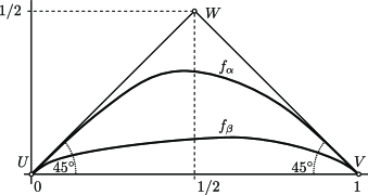
Figure 2. $f_{\alpha}$ and $f_{\beta}$ for $0<\alpha<\beta<1$

3. Proofs and further tools

3.1. More about finite convex geometries

Proof of Lemma 1.3.

For $X\subseteq E_{0}$, we have that

$$\Phi_{0}(\Phi_{0}(X)) =\Phi(\Phi(X)\cap E_{0})\cap E_{0}\subseteq\Phi(\Phi(X))\cap E_{0}$$

$$=\Phi(X)\cap E_{0}=\Phi_{0}(X).$$

Hence, it is straightforward to see that $\Phi_{0}$ satisfies Definition 1.1(i) and (iii); it suffices to deal only with 1.1(ii). In order to do so, assume that $A\in\textup{Pow}(E_{0})$, or $A\in\operatorname{\textup{Pow}_{\textup{fin}}}(E_{0})$, and let $x,y\in E_{0}\setminus\Phi_{0}(A)$ such that $\Phi_{0}(A\cup\{x\})=\Phi_{0}(A\cup\{y\})$. Since $x\in\Phi_{0}(A\cup\{x\})=\Phi_{0}(A\cup\{y\})\subseteq\Phi(A\cup\{y\})$, $A\subseteq\Phi(A\cup\{y\})$, and $\Phi$ is a closure operator, $\Phi(A\cup\{x\})\subseteq\Phi(\Phi(A\cup\{y\}))=\Phi(A\cup\{y\})$. Similarly, $\Phi(A\cup\{y\})\subseteq\Phi(A\cup\{x\})$, that is, $\Phi(A\cup\{y\})=\Phi(A\cup\{x\})$. Clearly, $x,y\notin\Phi(A)$. Applying  1.1(ii) to $\Phi$, it follows that $x=y$, as required. ∎

Proof of Lemma 1.4.

The “only if” part is included in Lemma 1.3. In order to show the “if” part, assume that all finite restrictions of $\langle E;\Phi\rangle$ are convex geometries. By the assumptions of the lemma, $\langle E;\Phi\rangle$ satisfies 1.1(i). Clearly, it also satisfies 1.1(iii). If $\langle E;\Phi\rangle$ failed to satisfy 1.2(iv) with $X$, $d$, and $d^{\prime}$, then ${\langle E;\Phi\rangle}\kern-1.0pt\rceil_{\kern-1.0ptX\cup\{d,d^{\prime}\}}$ would not be a convex geometry. ∎

Closure operators satisfying 1.1(iii) will be called zero-preserving. For a set $E$ and a subset $\mathfrak{G}$ of $\textup{Pow}(E)$, $\mathfrak{G}$ is a zero-preserving closure system on $E$ if $\emptyset,E\in\mathfrak{G}$ and $\mathfrak{G}$ is closed with respect to arbitrary intersections. As it is well-known, zero-preserving closure systems and zero-preserving closure operators on $E$ mutually determine each other. Namely, the map assigning $\mathfrak{G}_{\Phi}:=\{X\in\textup{Pow}(E):\Phi(X)=X\}$ to a zero-preserving closure operator $\Phi$ on $E$ and the map assigning $\Phi_{\mathfrak{G}}\colon\textup{Pow}(E)\to\textup{Pow}(E)$, defined by $\Phi_{\mathfrak{G}}(X):=\bigcap\{Y\in\mathfrak{G}:X\subseteq Y\}$, to a zero-preserving closure system $\mathfrak{G}$ on $E$ are reciprocal bijections.

Definition 3.1 (Alternative definition of finite convex geometries).

We say that $\langle E;\mathfrak{G}\rangle$ is a finite convex geometry if $E$ is finite and $\langle E;\Phi_{\mathfrak{G}}\rangle$ is a convex geometry in the sense of Definition 1.1.

From now on, the paragraph preceding Definition 3.1 enables us to use the notations $\langle E;\Phi\rangle$ and $\langle E;\mathfrak{G}\rangle$ for the same finite convex geometry interchangeably; then $\Phi$ and $\mathfrak{G}$ are understood as $\Phi_{\mathfrak{G}}$ and $\mathfrak{G}_{\Phi}$, respectively. The members of $\mathfrak{G}$ are called the closed sets of the convex geometry in question. Note that this abstract concept of closed sets corresponds to the geometric concept of convex sets. As usual, a partial ordering $\leq$ on a set $E$ is linear if for every $x,y\in E$, we have $x\leq y$ or $y\leq x$. For simplicity, for a subset $X$ and an element $y$ of $E$, we will use the notation

$$X<y\overset{\textup{def}}{\iff}(\forall x\in X)\,(x<y).$$

Lemma 3.2 ($(\dagger)$ and Theorems 5.1 and 5.2 in Edelman and Jamison [12]).

(A) If $\,\leq_{1}$, …, $\leq_{t}$ are linear orderings on a finite set $E=\{1,2,\dots,n\}$ and we define $\mathfrak{G}$ as

(3.1) $$\mathfrak{G}:=\{\emptyset\}\cup\{X\in\textup{Pow}(E):(\forall y\in E\setminus X)\,(\exists i\in\{1,\dots,t\})\,(X<_{i}y)\},$$

then $\langle E;\mathfrak{G}\rangle$ is a convex geometry.

(B) Every finite convex geometry is isomorphic to some $\langle E;\mathfrak{G}\rangle$ such that $\mathfrak{G}$ is determined by finitely many linear orderings as in (3.1).

Note that essentially the same statement is derived in Adaricheva and Czédli [1] from a lattice theoretical result. Note also that the minimum number of linear orderings that we need to represent a finite convex geometry according to (B) is the convex dimension of the convex geometry. Finiteness could be dropped from part (A). However, the technical assumption that $E$ is of the form $\{1,\dots,n\}$ will be convenient in the proof of Theorem 1.8. We will only use part (B). Since its proof is short and we have formulated the above statement a bit differently from [12], we present the argument below.

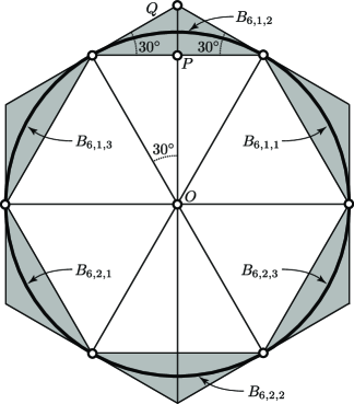
Figure 3. The unit circle with inscribed and circumscribed regular $t$-gons and $mt=6$ circular arcs

Proof of Lemma 3.2(B).

Let $\langle E;\mathfrak{G}^{\prime}\rangle$ be a finite convex geometry. Without loss of generality, we can assume that $E=\{1,\dots,n\}$. With respect to set inclusion, $\mathfrak{G}^{\prime}$ is a lattice. Assume that $X\prec Y$ in this lattice, and let $a,b\in Y\setminus X$. Since $Y$ covers $X$, $\Phi(X\cup\{a\})=Y=\Phi(X\cup\{b\})$. The anti-exchange property gives that $a=b$, whereby $Y\setminus X$ is a singleton. Hence, for $X,Y\in\mathfrak{G}^{\prime}$,

(3.2) $$X\prec Y\text{ in the lattice }\mathfrak{G}^{\prime}\text{ if{}f }X\subset Y\text{ and }|Y\setminus X|=1.$$

Consequently, all maximal chains in $\mathfrak{G}^{\prime}$ are of length $n=|E|$. Let $C_{1},\dots,C_{t}$ be a list of all maximal chains in $\mathfrak{G}^{\prime}$. By (3.2), $C_{i}$ is of the form

$$C_{i}=\bigl{\{}\emptyset,\{e_{i,1}\},\{e_{i,1},e_{i,2}\},\dots,\{e_{i,1},e_{i,2},\dots,e_{i,n}\}\bigr{\}},$$

for $i\in\{1,\dots,t\}$. This allows us to define a linear ordering $\leq_{i}$ on $E$ as follows:

$$e_{i,1}<_{i}e_{i,2}<_{i}e_{i,3}<_{i}\dots<_{i}e_{i,n},$$

for $i\in\{1,\dots,t\}$. Let $\mathfrak{G}$ denote what (3.1) defines from these linear orderings; we need to show that $\mathfrak{G}^{\prime}=\mathfrak{G}$. Note that $\emptyset\in\mathfrak{G}\cap\mathfrak{G}^{\prime}$. First, assume that $\emptyset\neq X\in\mathfrak{G}^{\prime}$. As every element in a finite lattice, $X$ belongs to a maximal chain $C_{i}$. So $X$ is of the form $\{e_{i,1},e_{i,2},\dots,e_{i,j}\}$, and the same subscript $i$ witnesses that $X\in\mathfrak{G}$.

Second, assume that $\emptyset\neq X\in\mathfrak{G}$. For each $y\in E\setminus X$, (3.1) allows us to pick an $i=i(y)$ such that $X<_{i(y)}y$. Let $X_{y}:=\{e\in E:e<_{i(y)}y\}$; it belongs to $C_{i(y)}$, whence $X_{y}\in\mathfrak{G}^{\prime}$. Let $Z:=\bigcap\{X_{y}:y\in E\setminus X\}$. Since $\mathfrak{G}^{\prime}$, like every closure system, is $\bigcap$-closed, $Z\in\mathfrak{G}^{\prime}$. Since all the $X_{y}$ include $X$, we have that $X\subseteq Z$. For each $y\in E\setminus X$, $y\notin X_{y}\supseteq Z$ gives that $y\notin Z$. This shows that $X\not\subset Z$. Hence, $X=Z\in\mathfrak{G}^{\prime}$, as required. ∎

3.2. Almost-circles and their accuracies

Definition 3.3.

For integers $t\geq 3$ and $m\in\mathbb{N}$ and an $m$-by-$t$ matrix $S=(s_{i,j})_{m\times t}$ of real numbers from $(0,1)$, we define a simple closed curve $C({{}^{\scriptscriptstyle{\textup{gf}}}\kern-2.2ptF},S)$ as follows; see Figures 2–4, where $m=2$, $t=3$, $\alpha<\beta$, and

(3.3) $$S=\begin{pmatrix}\alpha&\alpha&\beta\cr\alpha&\beta&\beta\end{pmatrix}.$$

Note in advance that $m$ plays the role of some sort of multiplicity of the almost-circle we are going to define; it will turn out later that the smaller $\epsilon$ is, the larger multiplicity is needed to achieve the accuracy of $1-\epsilon$. We start with the unit circle $\{\langle x,y\rangle:x^{2}+y^{2}=1\}$; see Figure 3. For $i\in\{1,\dots,m\}$ and $j\in\{1,\dots,t\}$, let $B_{mt,i,j}$ denote the arc of this circle with endpoints

(3.4) $$\Big{\langle}\kern-2.0pt\cos\frac{2\pi\cdot(m(i-1)+j-1)}{mt},\sin\frac{2\pi\cdot(m(i-1)+j-1)}{mt}\Big{\rangle}\,\text{ and}$$

(3.5) $$\Big{\langle}\kern-2.0pt\cos\frac{2\pi\cdot(m(i-1)+j)}{mt},\sin\frac{2\pi\cdot(m(i-1)+j)}{mt}\Big{\rangle}.$$

The secant and the tangent lines of this arc through its endpoints form an isosceles triangle $B^{\triangle}_{mt,i,j}$. These triangles are grey-filled in Figure 3. Neither $B^{\triangle}_{mt,i,j}$, nor $\triangle(U,V,W)$ in Figure 2 is a degenerate triangle. Hence, for every for $\langle i,j\rangle\in\{1,\dots,m\}\times\{1,\dots,t\}$, there exists a unique non-degenerate affine transformation $\psi_{mt,i,j}\colon\mathbb{R}^{2}\to\mathbb{R}^{2}$ mapping $\triangle(U,V,W)$ onto $B^{\triangle}_{mt,i,j}$ such that $V$ and $U$ are mapped to the endpoints (3.4) and (3.5), respectively. We let

(3.6) $$A_{S,i,j}=\psi_{mt,i,j}(\textup{Graph}(f_{s_{i,j}}));$$

remember that $f_{s_{i,j}}\in{{}^{\scriptscriptstyle{\textup{gf}}}\kern-2.2ptF}$ was defined in (2.3); see also Lemma 2.4. The closed curve formed by these $A_{S,i,j}$ will be denoted by $C({{}^{\scriptscriptstyle{\textup{gf}}}\kern-2.2ptF},S)$; see Figure 4. Note that, in order to increase the visibility of $C({{}^{\scriptscriptstyle{\textup{gf}}}\kern-2.2ptF},S)$, only one of the little triangles is fully grey and two others are partially grey in Figure 4.

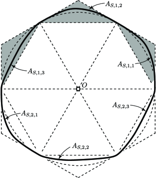
Figure 4. $C({{}^{\scriptscriptstyle{\textup{gf}}}\kern-2.2ptF},S)$, an almost-circle of accuracy $1-(\pi/6)^{2}\approx 0.7258$

Lemma 3.4.

$C({{}^{\scriptscriptstyle{\textup{gf}}}\kern-2.2ptF},S)$ defined in Definition 3.3 is an almost-circle of accuracy $1-(\pi/(mt))^{2}$.

Proof.

By (F3), the graphs of the $f_{s_{i,j}}$, for $\langle i,j\rangle\in\{1,\dots,m\}\times\{1,\dots,t\}$, are tangent at their endpoints to the legs of $\triangle(U,V,W)$; see Figure 2. Since this property is preserved by the transformations $\psi_{mt,i,j}$, see (3.6), and a leg of every little grey isosceles triangle in Figures 3 and 4 lies on the same line as a leg of the next little triangle, it follows that $C({{}^{\scriptscriptstyle{\textup{gf}}}\kern-2.2ptF},S)$ is differentiable where its arcs, the $A_{S,i,j}$, are joined. Elementary trigonometry yields that the ratio of $\overline{OP}$ and $\overline{OQ}$ is $\cos^{2}(\pi/(mt))=1-\sin^{2}(\pi/(mt))>1-(\pi/(mt))^{2}$; see Figure 3. Therefore, Lemma 2.4 and, thus, (F1)–(F6) imply Lemma 3.4 in a straightforward way. ∎

3.3. “Concentric” almost-circles at work

The title of this subsection only roughly describes its content, because an almost-circle does not have a well-defined center in general. However, only almost circles of the form $C({{}^{\scriptscriptstyle{\textup{gf}}}\kern-2.2ptF},S)$ will occur in this section, and an almost circle $C({{}^{\scriptscriptstyle{\textup{gf}}}\kern-2.2ptF},S)$ does have a unique center, which is the center of the corresponding unit circle; see Figure 3. Actually, we are going to use concentric almost-circles, which have the same center $\langle 0,0\rangle$.

We need the following construction; actually, it is a part of the subsequent lemma. This construction shows a lot of similarity with that given in Richter and Rogers [15], but we work with curves rather than vertices; actually, the number of our curves will be $m$ times more than the number of their vertices.

Definition 3.5.

For $n\in\mathbb{N}$, let $\vec{o}:=\langle\leq_{1},\dots,\leq_{t}\rangle$ be a $t$-tuple of linear orderings on the set $E=\{1,\dots,n\}$, and let $\langle E;\mathfrak{G}_{\eqref{eqGhzBfgdF}}\rangle$ be the convex geometry defined in (3.1). Let $m\in\mathbb{N}$, the multiplicity in the our construction, and let $K$ be a subset of the open interval $(0,1)$ of real numbers such that $|K|=mnt$. We order the Cartesian product $\{1,\dots,m\}\times\{1,\dots,t\}\times\{1,\dots,n\}$ lexicographically; for example, $\langle 1,1,3\rangle<_{\scriptscriptstyle{\textup{lex}}}\langle 1,2,1\rangle$. The three-fold Cartesian product above and $K$ are of the same size. Hence, equipped with $<_{\scriptscriptstyle{\textup{lex}}}$, this product is order isomorphic to $\langle K;<\rangle$, where $<$ is the usual ordering of real numbers. Thus, we can write $K$ in the form

(3.7) $$K=\{\alpha(i,j,k):\langle i,j,k\rangle\in\{1,\dots,m\}\times\{1,\dots,t\}\times\{1,\dots,n\}\} \alpha(i,j,k)<\alpha(i^{\prime},j^{\prime},k^{\prime}) \langle i,j,k\rangle<_{\scriptscriptstyle{\textup{lex}}}\langle i^{\prime},j^{\prime},k^{\prime}\rangle$$ such that iff .

For $e\in E$ and $j\in\{1,\dots,t\}$, let

(3.8) $$r(j,e)=|\{x\in E:e\leq_{j}x\}|.$$

That is, $r(j,e)$ denotes the position of $e$ according to the $j$-th ordering and counted backwards. Associated with $e\in E$, we define an

(3.9) $$m t S(e)=S(m,\vec{o},K;e)=(s_{i,j}(e))_{m\times t} s_{i,j}(e):=\alpha(i,j,r(j,e))\in K$$-by- matrix by the rule .

Using the almost-circles $C({{}^{\scriptscriptstyle{\textup{gf}}}\kern-2.2ptF},S(m,\vec{o},K;e))$ constructed in Definition 3.3, we let

(3.10) $$E_{\eqref{eqtxtdhNBmTrbBcB}}=\{C({{}^{\scriptscriptstyle{\textup{gf}}}\kern-2.2ptF},S(m,\vec{o},K;e)):e\in E\} \textup{Conv}_{E_{\eqref{eqtxtdhNBmTrbBcB}}}\colon\textup{Pow}(E_{\eqref{eqtxtdhNBmTrbBcB}})\to\textup{Pow}(E_{\eqref{eqtxtdhNBmTrbBcB}}) \mathfrak{G}_{\eqref{eqtxtdhNBmTrbBcB}}:=\{X\subseteq\textup{Pow}(E_{\eqref{eqtxtdhNBmTrbBcB}}):X=\textup{Conv}_{E_{\eqref{eqtxtdhNBmTrbBcB}}}(X)\}$$ and, with given in (1.3), we let .

Remark 3.6.

With the notation of Definition 3.5, for each $\beta\in K$, there exists a unique triplet $\langle i,j,e\rangle\in\{1,\dots,m\}\times\{1,\dots,t\}\times E$ such that $s_{i,j}(e)$, the $\langle i,j\rangle$-th entry of $S(m,\vec{o},K;e)$, is $\beta$. Indeed, there is a unique triplet $\langle i,j,k\rangle$ such that $\beta=\alpha(i,j,k)$, and, by (3.9), $e$ is the $(n+1-k)$-th element of $E$ with respect to $\leq_{j}$.

Lemma 3.7.

With the notation of Definition 3.5, $\langle E_{\eqref{eqtxtdhNBmTrbBcB}};\mathfrak{G}_{\eqref{eqtxtdhNBmTrbBcB}}\rangle$ is a convex geometry and it is isomorphic to $\langle E;\mathfrak{G}_{\eqref{eqGhzBfgdF}}\rangle$.

Proof.

Letting $H(e)=C({{}^{\scriptscriptstyle{\textup{gf}}}\kern-2.2ptF},S(m,\vec{o},K;e))$, we define a surjective map $H$ from $E=\{1,\dots,n\}$ to $E_{\eqref{eqtxtdhNBmTrbBcB}}$. Let $i\in\{1,\dots,m\}$ and $j\in\{1,\dots,t\}$, and assume that $e_{1}$ and $e_{2}$ are distinct elements of $E$. Then either $e_{1}<_{j}e_{2}$ or $e_{2}<_{j}e_{1}$. Hence $r(j,e_{1})\neq r(j,e_{2})$. It follows from (3.7) and (3.9) that $s_{i,j}(e_{1})=\alpha(i,j,r(j,e_{1}))\neq\alpha(i,j,r(j,e_{2}))=s_{i,j}(e_{2})$. Hence, Definition 3.3 and (F5), or even (F4), yield that $H(e_{1})$ is distinct from $H(e_{2})$; actually, they do not even have an arc in common. Thus, $H$ is injective and it is a bijection.

Next, we are going to show that, for every $X$,

(3.11) $$\text{if }X\in\textup{Pow}(E)\setminus\mathfrak{G}_{\eqref{eqGhzBfgdF}}\text{, then }H(X)\in\textup{Pow}(E)\setminus\mathfrak{G}_{\eqref{eqtxtdhNBmTrbBcB}}.$$

We know from (3.1) that $\emptyset\in\mathfrak{G}_{\eqref{eqGhzBfgdF}}$, whereby we can assume that $X\neq\emptyset$. Since $X\notin\mathfrak{G}_{\eqref{eqGhzBfgdF}}$, (3.1) yields a $y\in E\setminus X$ such that for all $j\in\{1,\dots,t\}$, $X\nless_{j}y$. Hence, for each $j\in\{1,\dots,t\}$, we can pick an $e_{j}\in X$ such that $y<_{j}e_{j}$. By (3.8), $r(j,y)>r(j,e_{j})$. Hence, (3.7) and (3.9) give that $s_{i,j}(y)>s_{i,j}(e_{j})$ holds for all $i\in\{1,\dots,m\}$ and $j\in\{1,\dots,t\}$. By (F4) and Definition 3.3, the $\langle i,j\rangle$-th arc $A_{S(m,\vec{o},K;y),i,j}$ of $H(y)=C({{}^{\scriptscriptstyle{\textup{gf}}}\kern-2.2ptF},S(m,\vec{o},K;y))$ is closer to the center $O:=\langle 0,0\rangle$ of the unit circle than the $\langle i,j\rangle$-th arc $A_{S(m,\vec{o},K;e_{j}),i,j}$ of $H(e_{j})=C({{}^{\scriptscriptstyle{\textup{gf}}}\kern-2.2ptF},S(m,\vec{o},K;e_{j}))$. Here, “closer” means that only the endpoints are in common but for every inner point $P$ of the second arc, the line segment $\overline{OP}$ has an inner point lying on the interior of the first arc. Therefore, $H(y)\in\textup{Conv}_{E_{\eqref{eqtxtdhNBmTrbBcB}}}\{H(e_{j}):j\in\{1,\dots,t\}\}\subseteq\textup{Conv}_{E_{\eqref{eqtxtdhNBmTrbBcB}}}(H(X))$. However, $y\notin X$ and the injectivity of $H$ give that $H(y)\notin H(X)$. This indicates that $H(X)$ is not closed with respect to $\textup{Conv}_{E_{\eqref{eqtxtdhNBmTrbBcB}}}$. Thus, $H(X)\notin\mathfrak{G}_{\eqref{eqtxtdhNBmTrbBcB}}$, proving (3.11).

Next, we are going to show converse implication, that is,

(3.12) $$\text{if }X\in\mathfrak{G}_{\eqref{eqGhzBfgdF}}\text{, then }H(X)\in\mathfrak{G}_{\eqref{eqtxtdhNBmTrbBcB}}.$$

Assume that $X\in\mathfrak{G}_{\eqref{eqGhzBfgdF}}$. In order to verify (3.12), we need to show that for every $y^{\prime}\in E_{\eqref{eqtxtdhNBmTrbBcB}}\setminus H(X)$, we have that $y^{\prime}\notin\textup{Conv}_{E_{\eqref{eqtxtdhNBmTrbBcB}}}(H(X))$. Since $H$ is a bijection, $y^{\prime}=H(y)$ for a uniquely determined $y\in E\setminus X$. Applying (3.1) to this $y$, we obtain a $j\in\{1,\dots,t\}$ such that $X<_{j}y$. Hence, for every $e\in X$, $e<_{j}y$. Thus, (3.8) gives that $r(j,e)>r(j,y)$. Combining this with (3.7) and (3.9), we conclude that, for all $i\in\{1,\dots,m\}$, $s_{i,j}(e)>s_{i,j}(y)$. (Actually, one such $i$ is sufficient in the present argument.) By (F4) and Definition 3.3, the $\langle i,j\rangle$-th arc $A_{S(m,\vec{o},K;e),i,j}$ of $H(e)=C({{}^{\scriptscriptstyle{\textup{gf}}}\kern-2.2ptF},S(m,\vec{o},K;e))$ is closer to the center $O:=\langle 0,0\rangle$ than the $\langle i,j\rangle$-th arc $A_{S(m,\vec{o},K;y),i,j}$ of $H(y)=C({{}^{\scriptscriptstyle{\textup{gf}}}\kern-2.2ptF},S(m,\vec{o},K;y))$. This means that the $\langle i,j\rangle$-th arc of $H(y)$ is “outside” $H(e)$ for all $e\in X$. That is, the $\langle i,j\rangle$-th curve of $H(y)$ is outside all members of $H(X)$. Consequently, $y^{\prime}=H(y)\notin\textup{Conv}_{E_{\eqref{eqtxtdhNBmTrbBcB}}}(H(X))$, as required. This proves (3.12). Finally, (3.11) and (3.12) imply that the bijection $H$ is actually an isomorphism, proving Lemma 3.7. ∎

3.4. The rest of the proof

We are going to define an appropriate set $T_{\textup{new}}$ needed by Theorem 1.8. Consider the set $U$ of all triplets $\langle n,\vec{o},m\rangle$ where

1. $n$ and $m$ are positive integers;

2. $\vec{o}=\langle\leq_{1},\leq_{2},\dots,\leq_{t}\rangle$ is a nonempty tuple of finitely many linear orderings on the set $E:=\{1,\dots,n\}$; the number of its components is $\dim(\vec{o})=t\in\mathbb{N}$.

Since $U$ is a countably infinite set, we obtain from basic cardinal arithmetic that $|\mathbb{R}|\cdot|U|=|(0,1)|$. This allows us to partition the real interval $(0,1)$ as a union $(0,1)=\bigcup\{I_{n,\vec{o},m}:\langle n,\vec{o},m\rangle\in U\}$ of pairwise disjoint subsets such that $|I_{n,\vec{o},m}|=2^{\aleph_{0}}$ for all $\langle n,\vec{o},m\rangle\in U$. Note that if we wrote the elements of $(0,1)$ into unique decimal forms not ending with $999\dots$ (infinitely many), then Cantor’s well-known method together with lots of technicalities would allow us to define $I_{n,\vec{o},m}$ and, eventually, $T_{\textup{new}}$ uniquely. However, we do not seek uniqueness; our only goal is to prove the existence of an appropriate $T_{\textup{new}}$. In the next step, using the equality $|\mathbb{R}|\cdot n\cdot\dim(\vec{o})\cdot m=2^{\aleph_{0}}=|I_{n,\vec{o},m}|$, which is trivial from cardinal arithmetic, we can partition $I_{n,\vec{o},m}$ as the union $I_{n,\vec{o},m}=\bigcup\{K_{\kappa,n,\vec{o},m}:\langle\kappa,\langle n,\vec{o},m\rangle\rangle\in\mathbb{R}\times U\}$ of pairwise disjoint $n\cdot\dim(\vec{o})\cdot m$-element subsets of $I_{n,\vec{o},m}$. In order to ease the notation, we will write $\langle\kappa,n,\vec{o},m\rangle$ rather than $\langle\kappa,\langle n,\vec{o},m\rangle\rangle$. Then, clearly,

(3.13) for every $$\langle\kappa,n,\vec{o},m\rangle\in\mathbb{R}\times U K_{\kappa,n,\vec{o},m}\subset(0,1) |K_{\kappa,n,\vec{o},m}|=n\cdot\dim(\vec{o})\cdot m \langle\kappa,n,\vec{o},m\rangle\neq\langle\kappa^{\prime},n^{\prime},\vec{o}\kern 1.0pt^{\prime},m^{\prime}\rangle K_{\kappa,n,\vec{o},m} K_{\kappa^{\prime},n^{\prime},\vec{o}\kern 1.0pt^{\prime},m^{\prime}}$$, and , and whenever , then is disjoint from .

Next, with the almost-circles $C({{}^{\scriptscriptstyle{\textup{gf}}}\kern-2.2ptF},S(m,\vec{o},K_{\kappa,n,\vec{o},m};e))$ from (3.10), we let

(3.14) $$T_{\textup{new}}:= \{\psi\bigl{(}C({{}^{\scriptscriptstyle{\textup{gf}}}\kern-2.2ptF},S(m,\vec{o},K_{\kappa,n,\vec{o},m};e))\bigr{)}:\langle\kappa,n,\vec{o},m\rangle\in\mathbb{R}\times U,$$

$$\phantom{\{}e\in\{1,\dots,n\},\text{ and }\psi\colon\mathbb{R}^{2}\to\mathbb{R}^{2}\text{ is a non-degenerate }$$

$$\phantom{\{}\text{affine transformation}\}\,\cup\,\{\{\vec{p}\}:\vec{p}\in\mathbb{R}^{2}\}.$$

Now, we are in the position to prove our theorem.

Proof of Theorem 1.8.

The $C({{}^{\scriptscriptstyle{\textup{gf}}}\kern-2.2ptF},S(m,\vec{o},K_{\kappa,n,\vec{o},m};e))$ in (3.14) are almost circles by Lemma 3.4. Hence, by Definition 1.6, they are differentiable convex simple closed planar curves. So are their images by non-degenerate affine transformations, proving part (i) of the theorem.

Part (iii) is a trivial consequence of (3.14), since the composite of two non-degenerate affine transformations is again a non-degenerate affine transformation.

In order to prove part (iv), take an arbitrary finite convex geometry and a positive $\epsilon<1$. By Lemma 3.2, we can assume that this convex geometry is given on a set $\{1,\dots,n\}$ with the help of a $\dim(\vec{o})$-tuple $\vec{o}$ of linear orderings on $\{1,\dots,n\}$; see (3.1). Pick an $m\in\mathbb{N}$ such that $m\geq\pi\cdot\dim(\vec{o}\kern 1.0pt)^{-1}\epsilon^{-1/2}$, and let $\kappa\in\mathbb{R}$. We also need $K_{\kappa,n,\vec{o},m}$; see (3.13). We apply Definition 3.5 and, in particular, (3.10), to $\langle n,m,\vec{o},K_{\kappa,n,\vec{o},m}\rangle$ instead of $\langle n,m,\vec{o},K\rangle$ in order to obtain $\langle E^{(\kappa,n,\vec{o},m)}_{\eqref{eqtxtdhNBmTrbBcB}},\mathfrak{G}^{(\kappa,n,\vec{o},m)}_{\eqref{eqtxtdhNBmTrbBcB}}\rangle$. Here,

(3.15) $$E^{(\kappa,n,\vec{o},m)}_{\eqref{eqtxtdhNBmTrbBcB}}=\{C({{}^{\scriptscriptstyle{\textup{gf}}}\kern-2.2ptF},S(m,\vec{o},K_{\kappa,n,\vec{o},m};e)):e\in\{1,\dots,n\}\}.$$

By Lemma 3.4, these almost-circles are of accuracy

$$1-(\pi/(m\cdot\dim(\vec{o}\kern 1.0pt))^{2} \geq 1-(\pi/(\pi\cdot\dim(\vec{o}\kern 1.0pt)^{-1}\epsilon^{-1/2}\cdot\dim(\vec{o}\kern 1.0pt))^{2}$$

$$=1-\epsilon.$$

By Lemma 3.7, $\langle E^{(\kappa,n,\vec{o},m)}_{\eqref{eqtxtdhNBmTrbBcB}},\mathfrak{G}^{(\kappa,n,\vec{o},m)}_{\eqref{eqtxtdhNBmTrbBcB}}\rangle$ is isomorphic to the arbitrary convex geometry we started with. This proves the first half of part (iv) of the Theorem. In order to prove the second half, suppose for a contradiction that $\langle\kappa,n,\vec{o},m\rangle$ and $\langle\kappa^{\prime},n^{\prime},\vec{o}\kern 1.0pt^{\prime},m^{\prime}\rangle$ are distinct quadruples of $\mathbb{R}\times U$ but $E^{(\kappa,n,\vec{o},m)}_{\eqref{eqtxtdhNBmTrbBcB}}$ is not affine-disjoint from $E^{(\kappa^{\prime},n^{\prime},\vec{o}\kern 1.0pt^{\prime},m^{\prime})}_{\eqref{eqtxtdhNBmTrbBcB}}$. Hence, there is an almost-circle $C_{1}$ in the first set and a non-degenerate affine transformation $\psi\colon\mathbb{R}^{2}\to\mathbb{R}^{2}$ such that $C_{2}:=\psi(C_{1})$ belongs to the second set. Since $C_{1}$ is one of the almost-circles occurring in (3.15), we know from (3.6) that its arcs are of the form $\psi_{m\dim(\vec{o}\kern 1.0pt),i,j}(\textup{Graph}(f_{s_{i,j}}))$. By (3.9) and (3.15), $\alpha:=s_{i,j}$ belongs to $K_{\kappa,n,\vec{o},m}$. Hence, the arcs of $C_{1}$ are non-degenerate affine images of finitely many graphs $\textup{Graph}(f_{\alpha_{1}})$, $\textup{Graph}(f_{\alpha_{2}})$, … such that $\alpha_{1},\alpha_{2},\dots$ belong to $K_{\kappa,n,\vec{o},m}$. By the same reason, the arcs of $C_{2}$ are non-degenerate affine images of finitely many graphs $\textup{Graph}(f_{\beta_{1}})$, $\textup{Graph}(f_{\beta_{2}})$, …with $\beta_{1},\beta_{2},\dots$ belonging to $K_{\kappa^{\prime},n^{\prime},\vec{o}\kern 1.0pt^{\prime},m^{\prime}}$. Since $\langle\kappa,n,\vec{o},m\rangle$ and $\langle\kappa^{\prime},n^{\prime},\vec{o}\kern 1.0pt^{\prime},m^{\prime}\rangle$ are distinct quadruples, we know from (3.13) that $\{\alpha_{1},\alpha_{2},\dots\}$ is disjoint from $\{\beta_{1},\beta_{2},\dots\}$. Since $\psi(C_{1})=C_{2}$, $\psi(\textup{Graph}(f_{\alpha_{1}}))$ and some of $\psi(\textup{Graph}(f_{\beta_{1}}))$, $\psi(\textup{Graph}(f_{\beta_{2}}))$,…have a nonempty open arc in common. Since $\alpha_{1}\notin\{\beta_{1},\beta_{2},\dots\}$, this common arc contradicts (F5). Therefore, part (iv) of the Theorem holds.

Next, before dealing with part (ii), we show that, for every $Y\subseteq T_{\textup{new}}$,

(3.16) $$\textup{Conv}_{\mathbb{R}^{2}}(\textup{Points}(Y))=\textup{Conv}_{\mathbb{R}^{2}}(\textup{Points}(\textup{Conv}_{T_{\textup{new}}}(Y))).$$

Using (1.3), we have that

Points $$(\textup{Conv}_{T_{\textup{new}}}(Y))\overset{\eqref{eqconvTanydef}}{=}\textup{Points}(\{D\in T_{\textup{new}}:D\subseteq\textup{Conv}_{\mathbb{R}^{2}}(\textup{Points}(Y))\})$$

$$\subseteq\textup{Points}(\{\textup{Conv}_{\mathbb{R}^{2}}(\textup{Points}(Y))\})=\textup{Conv}_{\mathbb{R}^{2}}(\textup{Points}(Y)).$$

Applying $\textup{Conv}_{\mathbb{R}^{2}}$ to both sides and using that $\textup{Conv}_{\mathbb{R}^{2}}\circ\textup{Conv}_{\mathbb{R}^{2}}=\textup{Conv}_{\mathbb{R}^{2}}$,

$$\textup{Conv}_{\mathbb{R}^{2}}(\textup{Points}(\textup{Conv}_{T_{\textup{new}}}(Y)))\subseteq\textup{Conv}_{\mathbb{R}^{2}}(\textup{Points}(Y)).$$

The converse inclusion also holds, because $\textup{Conv}_{T_{\textup{new}}}(Y)\supseteq Y$. This proves (3.16).

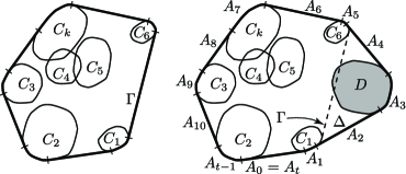
Figure 5. $\textup{Conv}_{T_{\textup{new}}}(\{C_{1},\dots,C_{k},D\})$ determines $D$, provided $D\notin\textup{Conv}_{T_{\textup{new}}}(\{C_{1},\dots,C_{k}\})$

From some aspects, the proof of part (ii) is analogous to that of Czédli [6, Proposition 2.1] for circles. If $D\in X\subseteq T_{\textup{new}}$, then $D\subseteq\textup{Points}(X)\subseteq\textup{Conv}_{\mathbb{R}^{2}}(\textup{Points}(X))$ gives that $D\in\textup{Conv}_{T_{\textup{new}}}(X)$. Hence, $X\subseteq\textup{Conv}_{T_{\textup{new}}}(X)$. Obviously, $\textup{Conv}_{T_{\textup{new}}}$ is monotone and zero-preserving. If $D\in\textup{Conv}_{T_{\textup{new}}}(\textup{Conv}_{T_{\textup{new}}}(X))$, then $D\in T_{\textup{new}}$ and

$$D\overset{\eqref{eqconvTanydef}}{\subseteq}\textup{Conv}_{\mathbb{R}^{2}}(\textup{Points}(\textup{Conv}_{T_{\textup{new}}}(X)))\overset{\eqref{eqcNvPnthnbnD}}{=}\textup{Conv}_{\mathbb{R}^{2}}(\textup{Points}(X)),$$

whereby $D\in\textup{Conv}_{T_{\textup{new}}}(X)$. Hence, $\textup{Conv}_{T_{\textup{new}}}(\textup{Conv}_{T_{\textup{new}}}(X))\subseteq\textup{Conv}_{T_{\textup{new}}}(X)$, and $\textup{Conv}_{T_{\textup{new}}}$ is a zero-preserving closure operator. That is, $\langle T_{\textup{new}};\textup{Conv}_{T_{\textup{new}}}\rangle$ satisfies Definition 1.1(i) and (iii). In order to show that it also satisfies Definition 1.2(iv), let $X=\{C_{1},\dots,C_{t}\}\subseteq T_{\textup{new}}$, $D,D^{\prime}\in T_{\textup{new}}$, and assume that $\textup{Conv}_{T_{\textup{new}}}(X\cup\{D\})=\textup{Conv}_{T_{\textup{new}}}(X\cup\{D^{\prime}\})$ and none of $D$ and $D^{\prime}$ belongs to $\textup{Conv}_{T_{\textup{new}}}(X)$. We need to give an affirmative answer to the question

(3.17) does $$\,D=D^{\prime}\,$$ hold?

By (1.3), none of $D$ and $D^{\prime}$ is a subset of $\textup{Conv}_{\mathbb{R}^{2}}(\textup{Points}(X))$. Let $\Gamma$ be the boundary of $\textup{Conv}_{\mathbb{R}^{2}}(\textup{Points}(X))$; see Figures 5 and 6. Note that in these two figures, $D$ is grey-filled but no $D^{\prime}$ distinct from $D$ is depicted. Singleton members of $X$ like $C_{2}$ in Figure  6 cause no problem.

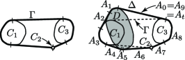
Figure 6. Two characteristic arcs, $A_{1}$ and $A_{5}$

We think of $\Gamma$ as a tight resilient rubber noose. Since $D\nsubseteq\textup{Conv}_{\mathbb{R}^{2}}(\textup{Points}(X))$, $D$ pushes $\Gamma$ outwards to obtain the boundary $\Delta$ of $\textup{Conv}_{\mathbb{R}^{2}}{(\textup{Points}(X\cup\{D\}))}$. It follows from (3.16) that $\Delta$ is also the boundary of $\textup{Conv}_{\mathbb{R}^{2}}{(\textup{Points}(X\cup\{D^{\prime}\}))}$. Hence, $D^{\prime}$ also pushes $\Gamma$ outwards to $\Delta$. Observe that $\Delta$ can be decomposed into arcs $A_{0},A_{1},\dots,A_{t-1},A_{t}=A_{0}$ of positive lengths; see Figures 5 and 6, and the same holds (with different $t$) for $\Gamma$. Keep in mind that our terminology concerning arcs allows straight line segments as special arcs. When distinction is necessary, we speak of straight line segments and non-straight arcs.

First, assume that one of $D$ and $D^{\prime}$ is a singleton. Let, say, $D$ be a singleton. Instead of a separate figure, take $X=\{C_{1},C_{3}\}$ and $D=C_{2}$ on the left of Figure 6 to see an example. Clearly, two straight line segments of $\Delta$, none of them being a part of a $\Gamma$-arc, form an angle with vertex $D$. This fact makes $D$ recognizable from $\Gamma$ and $\Delta$, and it follows that $D=D^{\prime}$. Hence, in the rest of the proof, we can assume that none of $D$ and $D^{\prime}$ is a singleton.

A non-straight arc of $\Delta$ will be called a characteristic arc (with respect to $\Gamma$) if it is neither a straight line segment, nor a subset of an arc of $\Gamma$. Necessarily, a characteristic arc is also an arc of $D$, and the same holds for $D^{\prime}$. Since $\Delta\neq\Gamma$ and none of $D$ and $D^{\prime}$ is a singleton, there is at least one characteristic arc. For example, the only characteristic arc in Figure 5 is $A_{3}$, but there are two characteristic arcs, $A_{1}$ and $A_{5}$, in Figure 6. Thus, $D$ and $D^{\prime}$ have an arc of positive length in common: a characteristic arc $I_{0}$ of $\Delta$. By (3.14), there exist $\langle\kappa,n,\vec{o},m\rangle$ and $\langle\kappa^{\prime},n^{\prime},\vec{o}\kern 1.0pt^{\prime},m^{\prime}\rangle$ in $\mathbb{R}\times U$, $e\in\{1,\dots,n\}$, $e^{\prime}\in\{1,\dots,n^{\prime}\}$, and non-degenerate affine transformations $\mu$ and $\mu^{\prime}$ such that

(3.18) $$D =\mu\bigl{(}C({{}^{\scriptscriptstyle{\textup{gf}}}\kern-2.2ptF},S(m,\vec{o},K_{\kappa,n,\vec{o},m};e))\bigr{)}\quad\text{and }$$

$$D^{\prime} =\mu^{\prime}\bigl{(}C({{}^{\scriptscriptstyle{\textup{gf}}}\kern-2.2ptF},S(m^{\prime},\vec{o}\kern 1.0pt^{\prime},K_{\kappa^{\prime},n^{\prime},\vec{o}\kern 1.0pt^{\prime},m^{\prime}};e^{\prime}))\bigr{)}.$$

Since $D$ and $D^{\prime}$ have the arc $I_{0}$ in common, their preimages,

$$C:=C({{}^{\scriptscriptstyle{\textup{gf}}}\kern-2.2ptF},S(m,\vec{o},K_{\kappa,n,\vec{o},m};e)) C^{\prime}:=C({{}^{\scriptscriptstyle{\textup{gf}}}\kern-2.2ptF},S(m^{\prime},\vec{o}\kern 1.0pt^{\prime},K_{\kappa^{\prime},n^{\prime},\vec{o}\kern 1.0pt^{\prime},m^{\prime}};e^{\prime}))$$ and ,

have arcs

(3.19) $$A:=A_{S(m,\vec{o},K_{\kappa,n,\vec{o},m};e),i,j}\,\text{ and }\,A^{\prime}:=A_{S(m^{\prime},\vec{o}\kern 1.0pt^{\prime},K_{\kappa^{\prime},n^{\prime},\vec{o}\kern 1.0pt^{\prime},m^{\prime}};e^{\prime}),i^{\prime},j^{\prime}},$$

respectively and in the sense of (3.6), such that the $I_{1}\subseteq\mu(A)$ and $I_{1}\subseteq\mu^{\prime}(A^{\prime})$ holds for some nonempty open sub-arc $I_{1}$ of $I_{0}$; necessarily of positive length. By the construction of our almost-circles in Definition 3.3, there are $\alpha,\alpha^{\prime}\in(0,1)$ and non-degenerate affine transformations $\varphi$ and $\varphi^{\prime}$ such that $A=\varphi(\textup{Graph}(f_{\alpha}))$ and $A^{\prime}=\varphi^{\prime}(\textup{Graph}(f_{\alpha^{\prime}}))$. Letting $\psi:=\mu\circ\varphi$ and $\psi^{\prime}:=\mu^{\prime}\circ\varphi^{\prime}$, we have that $I_{1}$ is a common open arc of both $\psi(\textup{Graph}(f_{\alpha}))$ and $\psi^{\prime}(\textup{Graph}(f_{\alpha^{\prime}}))$. It follows from (F5) that $\alpha=\alpha^{\prime}$ and $\psi=\psi^{\prime}$.

Roughly saying, disregarding $\psi$ in (3.14), $f_{\alpha}\in T_{\textup{new}}$ is used only once in the definition of $T_{\textup{new}}$, that is only in one almost-circle and only at one edge of this almost-circle; this implies that $\varphi=\varphi^{\prime}$. However, we give rigorous details below.

By the construction, see Definition 3.3, (3.9), and (3.14), $\alpha\in K_{\kappa,n,\vec{o},m}$ is an entry of the matrix $S:=S(m,\vec{o},K_{\kappa,n,\vec{o},m};e)$ and $\alpha^{\prime}\in K_{\kappa^{\prime},n^{\prime},\vec{o}\kern 1.0pt^{\prime},m^{\prime}}$ is that of $S^{\prime}:=S(m^{\prime},\vec{o}\kern 1.0pt,^{\prime}K_{\kappa^{\prime},n^{\prime},\vec{o}\kern 1.0pt^{\prime},m^{\prime}};e^{\prime})$. Since $\alpha=\alpha^{\prime}$, (3.13) yields that the quadruples $\langle\kappa,n,\vec{o},m\rangle$ and $\langle\kappa^{\prime},n^{\prime},\vec{o}\kern 1.0pt^{\prime},m^{\prime}\rangle$ are the same. Hence, using the equality $\alpha=\alpha^{\prime}$ together with Remark 3.6 for $\langle n,m,\vec{o},K_{\kappa,n,\vec{o},m}\rangle$ in the role of $\langle n,m,\vec{o},K\rangle$, we conclude that $S=S^{\prime}$, and there is a unique triplet $\langle i,j,e\rangle$ such that $\alpha$ is the $\langle i,j\rangle$-th entry of $S$. Furthermore, $S=S^{\prime}$ and $e=e^{\prime}$ give that $C=C^{\prime}$. Taking the uniqueness of $\langle i,j\rangle$ also into account, we obtain that $A=A^{\prime}$. The position of the $\langle i,j\rangle$-th arc in $C=C^{\prime}$ is uniquely determined by its endpoints given in (3.4) and (3.5). Therefore, $\varphi=\varphi^{\prime}$.

Finally, multiplying $\mu\circ\varphi=\psi=\psi^{\prime}=\mu^{\prime}\circ\varphi^{\prime}=\mu^{\prime}\circ\varphi$ by $\varphi^{-1}$ from the right, we obtain that $\mu=\mu^{\prime}$. Armed with $\mu=\mu^{\prime}$ and $C=C^{\prime}$, (3.18) gives that $D=D^{\prime}$, as required in (3.17). Thus, $T_{\textup{new}}$ satisfies Definition 1.2(iv). Hence, part (ii) of the theorem holds and the proof if complete. ∎

References

- [1] Adaricheva, K.; Czédli, G.: Note on the description of join-distributive lattices by permutations. Algebra Universalis 72, 155–162 (2014)
- [2] Adaricheva, K.; Nation, J.B.: Convex geometries. In Lattice Theory: Special Topics and Applications, volume 2, G. Grätzer and F. Wehrung, eds., Birkhäuser, 2015.
- [3] Adaricheva, K.; Nation, J.B.: A class if infinite convex geometries. arXiv:1501.04174
- [4] S.P. Avann: Application of the join-irreducible excess function to semimodular lattices. Math. Ann. 142, 345–354 (1961)
- [5] Czédli, G.: Coordinatization of join-distributive lattices. Algebra Universalis 71, 385–404 (2014)
- [6] Czédli, G.: Finite convex geometries of circles. Discrete Math. 330, 61–75 (2014)
- [7] Czédli, G.: Large sets of lattices without order embeddings. Communications in Algebra 44, 668–679 (2016)
- [8] Czédli, G.: Jakubíková-Studenovská, D.: Large rigid sets of algebras with respect to embeddability. Mathematica Slovaca 66, 401–406 (2016)
- [9] Czédli, G.; Maróti, M.; Romanowska, A.B.: A dyadic view of rational convex sets. Comment. Math. Univ. Carolin. 55, 159–173 (2014)
- [10] R.P. Dilworth: Lattices with unique irreducible decompositions. Ann. of Math. (2) 41, 771–777 (1940)
- [11] Duquenne, V.: The core of finite lattices. Discrete Math. 88 133–147 (1991)
- [12] P. H. Edelman; R. E. Jamison: The theory of convex geometries. Geom. Dedicata 19, 247–271 (1985)
- [13] Kashiwabara, Kenji; Nakamura, Masataka; Okamoto, Yoshio: The affine representation theorem for abstract convex geometries. Comput. Geom. 30 129–144 (2005)
- [14] B. Monjardet: A use for frequently rediscovering a concept. Order 1, 415–417 (1985)
- [15] Richter, Michael; Rogers, Luke G.: Embedding convex geometries and a bound on convex dimension. Discrete Mathematics; accepted subject to minor changes; arXiv:1502.01941