EXPONENTIAL FOURIER COLLOCATION METHODS FOR SOLVING FIRST-ORDER DIFFERENTIAL EQUATIONS

Abstract

In this paper, a novel class of exponential Fourier collocation methods (EFCMs) is presented for solving systems of first-order ordinary differential equations. These so-called exponential Fourier collocation methods are based on the variation-of-constants formula, incorporating a local Fourier expansion of the underlying problem with collocation methods. We discuss in detail the connections of EFCMs with trigonometric Fourier collocation methods (TFCMs), the well-known Hamiltonian Boundary Value Methods (HBVMs), Gauss methods and Radau IIA methods. It turns out that the novel EFCMs are an essential extension of these existing methods. We also analyse the accuracy in preserving the quadratic invariants and the Hamiltonian energy when the underlying system is a Hamiltonian system. Other properties of EFCMs including the order of approximations and the convergence of fixed-point iterations are investigated as well. The analysis given in this paper proves further that EFCMs can achieve arbitrarily high order in a routine manner which allows us to construct higher-order methods for solving systems of first-order ordinary differential equations conveniently. We also derive a practical fourth-order EFCM denoted by EFCM(2,2) as an illustrative example. The numerical experiments using EFCM(2,2) are implemented in comparison with an existing fourth-order HBVM, an energy-preserving collocation method and a fourth-order exponential integrator in the literature. The numerical results demonstrate the remarkable efficiency and robustness of the novel EFCM(2,2).

5L05, 65L20, 65M20, 65M70.

1 Introduction

This paper is devoted to analysing and designing novel and efficient numerical integrators for solving the following first-order initial value problems

$$u^{\prime}(t)+Au(t)=g(t,u(t)),\qquad u(0)=u_{0},\qquad t\in[0,t_{\mathrm{end}}],$$ (1)

where $g:\mathbb{R}\times\mathbb{R}^{d}\rightarrow\mathbb{R}^{d}$ is an analytic function, $A$ is assumed to be a linear operator on a Banach space $X$ with a norm $\left\|\cdot\right\|$, and $(-A)$ is the infinitesimal generator of a strongly continuous semigroup $e^{-tA}$ on $X$ (see, e.g. [27]). This assumption of $A$ means that there exist two constants $C$ and $\omega$ satisfying

$$\left\|e^{-tA}\right\|_{X\leftarrow X}\leq Ce^{\omega t},\ \ \ \ \ t\geq 0.$$ (2)

An analysis about this result can be found in [27]. It is noted that if $X$ is chosen as $X=\mathbb{R}^{d}$ or $X=\mathbb{C}^{d}$, then the linear operator $A$ can be expressed by a $d\times d$ matrix. Accordingly in this case, $e^{-tA}$ is exactly the matrix exponential function. It also can be observed that the condition (2) holds with $\omega=0$ provided the field of values of $A$ is contained in the right complex half-plane. In the special and important case where $A$ is skew-Hermitian or Hermitian positive semidefinite, we have $C=1$ and $\omega=0$ in the Euclidean norm, independently of the dimension $d$. If $A$ originates from a spatial discretisation of a partial differential equation, then the assumption of $A$ leads to temporal convergence results that are independent of the spatial mesh.

It is known that the exact solution of (1) can be represented by the variation-of-constants formula

$$u(t)=e^{-tA}u_{0}+\int_{0}^{t}e^{-(t-\tau)A}g(\tau,u(\tau))d\tau.\\$$ (3)

For oscillatory problems, the exponential subsumes the full information on linear oscillations. This class of problems (1) frequently rises in a wide variety of applications including engineering, mechanics, quantum physics, circuit simulations, flexible body dynamics and other applied sciences (see, e.g. [10, 16, 24, 27, 39, 41, 44, 47]). Parabolic partial differential equations with their spatial discretisations and highly oscillatory problems are two typical examples of the system (1) (see, e.g. [30, 31, 32, 33, 34, 42]). Linearizing stiff systems $u^{\prime}(t)=F(t,u(t))$ also yields examples of the form (1)(see, e.g. [15, 25, 28]).

Based on the variation-of-constants formula (3), the numerical scheme for (1) is usually constructed by incorporating the exact propagator of (1) in an appropriate way. For example, interpolating the nonlinearity at the known value $g(0,u_{0})$ yields the exponential Euler approximation for (3). Approximating the functions arising by rational approximations leads to implicit or semi-implicit Runge–Kutta methods, Rosenbrock methods or W-schemes. Recently, the construction, analysis, implementation and application of exponential integrators have been studied by many researchers, and we refer the reader to [3, 11, 12, 13, 16, 37, 45], for example. Exponential integrators make explicit use of the quantity $Au$ of (1), and a systematic survey of exponential integrators is referred to [27].

Based on Lagrange interpolation polynomials, exponential Runge-Kutta methods of collocation type are constructed and their convergence properties are analysed in [26]. In [40], the authors developed and researched a novel type of trigonometric Fourier collocation methods (TFCMs) for second-order oscillatory differential equations $q^{\prime\prime}(t)+Mq(t)=f(q(t))$ with a principal frequency matrix $M\in\mathbb{R}^{d\times d}$. These new trigonometric Fourier collocation methods take full advantage of the special structure brought by the linear term $Mq$, and its construction incorporates the idea of collocation methods, the variation-of-constants formula and the local Fourier expansion of the system. The results of numerical experiments in [40] showed that the trigonometric Fourier collocation methods are much more efficient in comparison with some alternative approaches that have previously appeared in the literature. On the basis of the work in [26, 40], in this paper we make an effort to conduct the research of novel exponential Fourier collocation methods (EFCMs) for efficiently solving first-order differential equations (1). The construction of the novel EFCMs incorporates the exponential integrators, the collocation methods, and the local Fourier expansion of the system. Moveover, EFCMs can be of an arbitrarily high order, and when $A\rightarrow 0$, EFCMs reduce to the well-known Hamiltonian Boundary Value methods (HBVMs) which have been studied by many researchers (see, e.g. [6, 7, 8]). It is also shown in this paper that EFCMs are an extension of Gauss methods, Radau IIA methods and TFCMs.

The paper is organized as follows. We first formulate the scheme of EFCMs in Section 2. Section 3 discusses the connections of the novel EFCMs with HBVMs, Gauss methods, Radau IIA methods and TFCMs. In Section 4, we analyse the properties of EFCMs. Section 5 is concerned with constructing a practical EFCM and reporting four numerical experiments to demonstrate the excellent qualitative behavior of the novel approximation. Section 6 includes some conclusions.

2 Formulation of EFCMs

In this section, we present the formulation of exponential Fourier collocation methods (EFCMs) for systems of first-order differential equations (1).

2.1 Local Fourier expansion

We first restrict the first-order differential equations (1) to the interval $[0,h]$ with any $h>0$:

$$u^{\prime}(t)+Au(t)=g(t,u(t)),\qquad u(0)=u_{0},\qquad t\in[0,h].$$ (4)

Consider the shifted Legendre polynomials $\{\widehat{P}_{j}\}_{j=0}^{\infty}$ satisfying

$$\int_{0}^{1}\widehat{P}_{i}(x)\widehat{P}_{j}(x)dx=\delta_{ij},\qquad\deg\big{(}\widehat{P}_{j}\big{)}=j,\qquad i,j\geq 0,$$

where $\delta_{ij}$ is the Kronecker symbol. We then expand the right-hand-side function of (4) as follows:

$$g(\xi h,u(\xi h))=\sum\limits_{j=0}^{\infty}\widehat{P}_{j}(\xi)\kappa_{j}(h,u),\ \ \xi\in[0,1];\ \ \kappa_{j}(h,u):=\int_{0}^{1}\widehat{P}_{j}(\tau)g(\tau h,u(\tau h))d\tau.$$ (5)

The system (4) now can be rewritten as

$$u^{\prime}(\xi h)+Au(\xi h)=\sum\limits_{j=0}^{\infty}\widehat{P}_{j}(\xi)\kappa_{j}(h,u),\qquad u(0)=u_{0}.$$ (6)

The next theorem gives its solution.

Theorem 2.1.

The solution of (4) can be expressed by

$$u(t)=\varphi_{0}(-tA)u_{0}+t\sum\limits_{j=0}^{\infty}I_{j}(tA)\kappa_{j}(t,u),$$ (7)

where $t\in[0,h]$ and

$$I_{j}(tA):=\int_{0}^{1}\widehat{P}_{j}(z)e^{-(1-z)tA}dz=\sqrt{2j+1}\sum\limits_{k=0}^{j}(-1)^{j+k}\frac{(j+k)!}{k!(j-k)!}\varphi_{k+1}(-tA).$$ (8)

Here the $\varphi$-functions (see, e.g. [24, 25, 27, 28]) are defined by:

$$\varphi_{0}(z)=e^{z},\ \ \varphi_{k}(z)=\int_{0}^{1}e^{(1-\sigma)z}\frac{\sigma^{k-1}}{(k-1)!}d\sigma,\ \ k=1,2,\ldots.$$

Proof 2.2.

It follows from the variation-of-constants formula (3) that

$$u(t) =e^{-tA}u_{0}+\int_{0}^{t}e^{-(t-\tau)A}g(\tau,u(\tau))d\tau$$

$$=\varphi_{0}(-tA)u_{0}+t\int_{0}^{1}e^{-(1-z)tA}g(zt,u(zt))dz.$$

Replacing the function $g(zt,u(zt))$ in the integral by (5) yields

$$u(t) =\varphi_{0}(-tA)u_{0}+t\int_{0}^{1}e^{-(1-z)tA}\sum\limits_{j=0}^{\infty}\widehat{P}_{j}(z)\kappa_{j}(t,u)dz$$

$$=\varphi_{0}(-tA)u_{0}+t\sum\limits_{j=0}^{\infty}\int_{0}^{1}\widehat{P}_{j}(z)e^{-(1-z)tA}dz\kappa_{j}(t,u),$$

which gives the formula (7) by letting $I_{j}(tA)=\int_{0}^{1}\widehat{P}_{j}(z)e^{-(1-z)tA}dz$.

According to the definition of shifted Legendre polynomials in the interval $[0,1]$:

$$\widehat{P}_{j}(x)=(-1)^{j}\sqrt{2j+1}\sum\limits_{k=0}^{j}{j\choose{k}}{j+k\choose{k}}(-x)^{k},\qquad j=0,1,\ldots,\qquad x\in[0,1],$$ (9)

we arrive at

$$I_{j}(tA)=\int_{0}^{1}\widehat{P}_{j}(z)e^{-(1-z)tA}dz$$

$$= \int_{0}^{1}(-1)^{j}\sqrt{2j+1}\sum\limits_{k=0}^{j}{j\choose{k}}{j+k\choose{k}}(-z)^{k}e^{-(1-z)tA}dz$$

$$= \sqrt{2j+1}\sum\limits_{k=0}^{j}(-1)^{j+k}{j\choose{k}}{j+k\choose{k}}\int_{0}^{1}z^{k}e^{-(1-z)tA}dz$$

$$= \sqrt{2j+1}\sum\limits_{k=0}^{j}(-1)^{j+k}\frac{(j+k)!}{k!(j-k)!}\varphi_{k+1}(-tA).$$

2.2 Discretisation

The authors in [8] made use of interpolation quadrature formulae and gave the discretisation for initial value problems. Following [8], two tools are coupled in this part. We first truncate the local Fourier expansion after a finite number of terms and then compute the coefficients of the expansion by a suitable quadrature formula.

We now consider truncating the Fourier expansion, a technique which originally appeared in [8]. This can be achieved by truncating the series (7) after $n$ ($n\geq 2$) terms with the stepsize $h$ and $V:=hA$:

$$\tilde{u}(h)=\varphi_{0}(-V)u_{0}+h\sum\limits_{j=0}^{n-1}I_{j}(V)\kappa_{j}(h,\tilde{u}),$$ (10)

which satisfies the following initial value problem:

$$\tilde{u}^{\prime}(\xi h)+A\tilde{u}(\xi h)=\sum\limits_{j=0}^{n-1}\widehat{P}_{j}(\xi)\kappa_{j}(h,\tilde{u}),\ \ \ \ \tilde{u}(0)=u_{0}.$$

The key challenge in designing practical methods is how to deal with $\kappa_{j}(h,\tilde{u})$ effectively. To this end, we introduce a quadrature formula using $k$ abscissae $0\leq c_{1}\leq\ldots\leq c_{k}\leq 1$ and being exact for polynomials of degree up to $m-1$. It is required that $m\geq k$ in this paper, and we note that many existed quadrature formulae satisfy this requirement, such as the well-known Gauss–Legendre quadrature and the Radau quadrature. We thus obtain an approximation of the form

$$\kappa_{j}(h,\tilde{u})\approx\sum\limits_{l=1}^{k}b_{l}\widehat{P}_{j}(c_{l})g(c_{l}h,\tilde{u}(c_{l}h)),\ \ \ \ j=0,1,\ldots,n-1,$$ (11)

where $b_{l}$ for $l=1,2,\ldots,k$ are the quadrature weights. It is noted that since the number of the integrals $\kappa_{j}(h,\tilde{u})$ is $n$, it is assumed that $k\geq n$. Therefore, we have $m\geq n$.

Since the quadrature is exact for polynomials of degree $m-1$, its remainder depends on the $m$-th derivative of the integrand $\widehat{P}_{j}(\tau)g(\tau h,u(\tau h))$ with respect to $\tau$. Consequently, the approximation gives

$$\Delta_{j}(h,\tilde{u}):=\kappa_{j}(h,\tilde{u})-\sum\limits_{l=1}^{k}b_{l}\widehat{P}_{j}(c_{l})g(c_{l}h,\tilde{u}(c_{l}h))$$

$$= \int_{0}^{1}\widehat{P}_{j}(\tau)g(\tau h,u(\tau h))d\tau-\sum\limits_{l=1}^{k}b_{l}\widehat{P}_{j}(c_{l})g(c_{l}h,\tilde{u}(c_{l}h))$$

$$= C\int_{0}^{1}\dfrac{d^{m}\Big{(}\widehat{P}_{j}(\tau)g(\tau h,u(\tau h))\Big{)}}{d\tau^{m}}|_{\tau=\zeta}d\tau,$$

where $C$ is a constant, and $\zeta\ (\zeta\in[0,1])$ depends on $\tau$. Taking account of $\widehat{P}^{(k)}_{j}(\tau)=0$ for $k>j$, we obtain

$$\Delta_{j}(h,\tilde{u})= C\int_{0}^{1}\widehat{P}_{j}(\zeta)\hat{g}^{(m)}(\zeta h)d\tau h^{m}+Cm\int_{0}^{1}\widehat{P}^{\prime}_{j}(\zeta)\hat{g}^{(m-1)}(\zeta h)d\tau h^{m-1}$$

$$+\cdots+C{m\choose{j}}\int_{0}^{1}\widehat{P}^{(j)}_{j}(\zeta)\hat{g}^{(m-j)}(\zeta h)d\tau h^{m-j}=\mathcal{O}(h^{m-j}),$$

$$\qquad\qquad\qquad\qquad\qquad\qquad\qquad\qquad\qquad\qquad j=0,1,\ldots,n-1$$

with the notation $\hat{g}^{(k)}(\zeta h)=g^{(k)}(\zeta h,u(\zeta h)).$ This guarantees that each $\Delta_{j}(h,\tilde{u})$ has good accuracy for any $j=0,1,\ldots,n-1$. Choosing $k$ large enough, along with a suitable choice of $c_{l},\ b_{l}$ for $\ l=1,2,\ldots,k$, allows us to approximate the given integral $\kappa_{j}(h,\tilde{u})$ to any degree of accuracy.

With (10) and (11), it is natural to consider the following numerical scheme

$$v(h)=\varphi_{0}(-V)u_{0}+h\sum\limits_{j=0}^{n-1}I_{j}(V)\sum\limits_{l=1}^{k}b_{l}\widehat{P}_{j}(c_{l})g(c_{l}h,v(c_{l}h)),$$

which exactly solves the initial value problem as follows:

$$v^{\prime}(\xi h)=-Av(\xi h)+\sum\limits_{j=0}^{n-1}\widehat{P}_{j}(\xi)\sum\limits_{l=1}^{k}b_{l}\widehat{P}_{j}(c_{l})g(c_{l}h,v(c_{l}h)),\ \ \ \ v(0)=u_{0}.$$ (12)

It follows from (12) that $v(c_{i}h)$ for $i=1,2,\ldots,k$ satisfy the following first-order differential equations:

$$v^{\prime}(c_{i}h)+Av(c_{i}h)=\sum\limits_{j=0}^{n-1}\widehat{P}_{j}(c_{i})\sum\limits_{l=1}^{k}b_{l}\widehat{P}_{j}(c_{l})g(c_{l}h,v(c_{l}h)),\ \ \ v(0)=u_{0}.$$ (13)

Letting $v_{i}=v(c_{i}h),$ (13) can be solved by the variation-of-constants formula (3) of the form:

$$v_{i}= \varphi_{0}(-c_{i}V)u_{0}+c_{i}h\sum\limits_{j=0}^{n-1}I_{j,c_{i}}(V)\sum\limits_{l=1}^{k}b_{l}\widehat{P}_{j}(c_{l})g(c_{l}h,v_{l}),\ \ \ i=1,2,\ldots,k,$$

where

$$I_{j,c_{i}}(V):=\int_{0}^{1}\widehat{P}_{j}(c_{i}z)e^{-(1-z)c_{i}V}dz$$ (14)

$$= \int_{0}^{1}(-1)^{j}\sqrt{2j+1}\sum\limits_{k=0}^{j}{j\choose{k}}{j+k\choose{k}}(-c_{i}z)^{k}e^{-(1-z)c_{i}V}dz$$

$$= (-1)^{j}\sqrt{2j+1}\sum\limits_{k=0}^{j}(-c_{i})^{k}{j\choose{k}}{j+k\choose{k}}\int_{0}^{1}z^{k}e^{-(1-z)c_{i}V}dz$$

$$= (-1)^{j}\sqrt{2j+1}\sum\limits_{k=0}^{j}(-c_{i})^{k}\frac{(j+k)!}{k!(j-k)!}\varphi_{k+1}(-c_{i}V).$$

2.3 The exponential Fourier collocation methods

We are now in a position to present the novel exponential Fourier collocation methods for systems of first-order differential equations (1).

Definition 2.3.

The $k$-stage exponential Fourier collocation method with an integer $n$ (denoted by EFCM(k,n)) for integrating systems of first-order differential equations (1) is defined by

$$v_{i}= \varphi_{0}(-c_{i}V)u_{0}+c_{i}h\sum\limits_{l=1}^{k}b_{l}\Big{(}\sum\limits_{j=0}^{n-1}I_{j,c_{i}}(V)\widehat{P}_{j}(c_{l})\Big{)}g(c_{l}h,v_{l}),\ i=1,2,\ldots,k,$$ (15)

$$v(h) =\varphi_{0}(-V)u_{0}+h\sum\limits_{l=1}^{k}b_{l}\Big{(}\sum\limits_{j=0}^{n-1}I_{j}(V)\widehat{P}_{j}(c_{l})\Big{)}g(c_{l}h,v_{l}),$$

where $h$ is the stepsize, $V:=hA$, $\widehat{P}_{j}$ for $j=0,1,\ldots,n-1$ are defined by (9), and $c_{l},\ b_{l}$ for $l=1,2,\ldots,k$ are the node points and the quadrature weights of a quadrature formula, respectively. Here, $n$ is an integer which is required to satisfy the condition: $2\leq n\leq k$. $I_{j}(V)$ and $I_{j,c_{i}}(V)$ are determined by

$$I_{j}(V)=\sqrt{2j+1}\sum\limits_{k=0}^{j}(-1)^{j+k}\frac{(j+k)!}{k!(j-k)!}\varphi_{k+1}(-V),$$

$$I_{j,c_{i}}(V)=(-1)^{j}\sqrt{2j+1}\sum\limits_{k=0}^{j}(-c_{i})^{k}\frac{(j+k)!}{k!(j-k)!}\varphi_{k+1}(-c_{i}V).$$

Remark 2.4.

Clearly, it can be observed that the EFCM(k,n) defined by (15) exactly integrates the homogeneous linear system $u^{\prime}+Au=0$, thus it is trivially A-stable. The EFCM(k,n) (15) approximates the solution of (1) in the time interval $[0,h]$. Obviously, the obtained result $v(h)$ can be considered as the initial condition for a new initial value problem and $u(t)$ can be approximated in the time interval $[h,2h]$. In general, the EFCM(k,n) can be extended to the approximation of the solution in an arbitrary interval $[0,Nh]$, where $N$ is a positive integer.

Remark 2.5.

The novel EFCM(k,n) (15) developed here is a kind of exponential integrator which requires the approximation of products of $\varphi$-functions with vectors. It is noted that if $A$ has a simple structure, it is possible to compute the $\varphi$-functions in a fast and reliable way. Moveover, many different approaches to evaluating this action in an efficient way have been proposed in the literature, see, e.g. [1, 2, 4, 22, 23, 27, 35, 36]. Furthermore, all the matrix functions appearing in the EFCM(k,n) (15) only need to be calculated once in the actual implementation for the given stepsize $h$. In Section 5, we will compare our novel methods with some traditional collocation methods (which do not require the evaluation of matrix functions) by four experiments. For each problem, we will display the work precision diagram in which the global error is plotted versus the execution time. The numerical results given in Section 5 demonstrate the efficiency of our novel approximation.

3 Connections with some existing methods

So far various effective methods have been developed for solving first-order differential equations and this section is devoted to exploring the connections between our novel EFCMs and some other existing methods in the literature. It turns out that some existing traditional methods can be gained by letting $A\rightarrow 0$ in the corresponding EFCMs or by applying EFCMs to special second-order differential equations.

3.1 Connections with HBVMs and Gauss methods

Hamiltonian Boundary Value methods (HBVMs) are an interesting class of integrators, which exactly preserve energy of polynomial Hamiltonian systems (see, e.g. [6, 7, 8]). We first consider the connection between EFCMs and HBVMs.

It can be observed that from (14) that when $A\rightarrow 0$, $I_{j}(V)$ and $I_{j,c_{i}}(V)$ in (15) become

$$\tilde{I}_{j}: =I_{j}(0)=\int_{0}^{1}\widehat{P}_{j}(z)dz=\left\{\begin{aligned} &1,\ j=0,\\ &0,\ j\geq 1,\end{aligned}\right.$$

$$\tilde{I}_{j,c_{i}}: =I_{j,c_{i}}(0)=\int_{0}^{1}\widehat{P}_{j}(c_{i}z)dz.$$

This can be summed up in the following result.

Theorem 3.1.

When $A\rightarrow 0$, the EFCM(k,n) defined by (15) reduces to

$$v_{i}= u_{0}+c_{i}h\sum\limits_{l=1}^{k}b_{l}\Big{(}\sum\limits_{j=0}^{n-1}\tilde{I}_{j,c_{i}}\widehat{P}_{j}(c_{l})\Big{)}g(c_{l}h,v_{l}),\ i=1,2,\ldots,k,$$ (16)

$$v(h) =u_{0}+h\sum\limits_{l=1}^{k}b_{l}g(c_{l}h,v_{l}),$$

which can be rewritten as a $k$-stage Runge-Kutta method with the following Butcher tableau

$$c_{1}$$

(17)

This method is exactly the Hamiltonian Boundary Value Method HBVM(k,n) using the discretisation researched in [6, 7, 8] for the first-order system

$$u^{\prime}(t)=g(t,u(t)),\ u(0)=u_{0}.$$

From the property of HBVM(k,n) given in [8], it follows that HBVM(k,k) reduces to a $k$-stage Gauss-Legendre collocation method when a Gaussian distribution of the nodes $(c_{1},\cdots,c_{k})$ is used. In view of this and as an straightforward consequence of Theorem 3.1, we obtain the connection between EFCMs and Gauss methods. This result is described below.

Theorem 3.2.

Under the condition that $c_{l},\ b_{l}$ for $l=1,2,\ldots,k$ are chosen respectively as the node points and the quadrature weights of a $k$-point Gauss–Legendre quadrature over the interval $[0,1]$, then the EFCM(k,k) defined by (15) reduces to the $k$-stage Gauss method presented in [19] when $A\rightarrow 0$.

3.2 Connection between EFCMs and Radau IIA methods

The following theorem states the connection between EFCMs and Radau IIA methods.

Theorem 3.3.

Choose $c_{l},\ b_{l}$ for $l=1,2,\ldots,k$ respectively as the node points and the weights of the Radau-right quadrature formula. Then the EFCM(k,k) defined by (15) reduces to a $k$-stage Radau IIA method presented in [20] when $A\rightarrow 0$.

Proof 3.4.

It follows from Theorem 3.1 that when $A\rightarrow 0,$ the EFCM(k,k) defined by (15) reduces to (16) with $n=k$. According to [20], the shifted Legendre polynomials $\{\widehat{P}_{j}\}_{j=0}^{\infty}$ satisfy the following integration formulae

$$\int_{0}^{x}\widehat{P}_{0}(t)dt=\xi_{1}\widehat{P}_{1}(x)+\frac{1}{2}\widehat{P}_{0}(x),$$

$$\int_{0}^{x}\widehat{P}_{m}(t)dt=\xi_{m+1}\widehat{P}_{m+1}(x)-\xi_{m}\widehat{P}_{m-1}(x),\ m=1,2,\ldots,k-2,$$

$$\int_{0}^{x}\widehat{P}_{k-1}(t)dt=\beta_{k}\widehat{P}_{k-1}(x)-\xi_{k-1}\widehat{P}_{k-2}(x),$$

where

$$\xi_{m}=\frac{1}{2\sqrt{4m^{2}-1}},\ \ \ \beta_{k}=\frac{1}{4k-2}.$$

These formulae imply

$$\bar{A}= \left(\begin{array}[]{ccc}\int_{0}^{c_{1}}\widehat{P}_{0}(\tau)d\tau&\ldots&\int_{0}^{c_{1}}\widehat{P}_{k-1}(\tau)d\tau\\ \vdots&&\vdots\\ \int_{0}^{c_{k}}\widehat{P}_{0}(\tau)d\tau&\ldots&\int_{0}^{c_{k}}\widehat{P}_{k-1}(\tau)d\tau\\ \end{array}\right)\left(\begin{array}[]{ccc}b_{1}\widehat{P}_{0}(c_{1})&\ldots&b_{s}\widehat{P}_{0}(c_{s})\\ \vdots&&\vdots\\ b_{1}\widehat{P}_{k-1}(c_{1})&\ldots&b_{s}\widehat{P}_{k-1}(c_{s})\\ \end{array}\right)$$

$$= WX_{k}Q,$$

where the matrix $W$ is defined by

$$\omega_{ij}=\widehat{P}_{j-1}(c_{i}),\ \ \ \ i,j=1,\ldots,k,$$

and the matrices $X_{k},\ Q$ are determined by

$$X_{k}=\left(\begin{array}[]{ccccc}\frac{1}{2}&-\xi_{1}&&&\\ \xi_{1}&0&-\xi_{2}&&\\ &\ddots&\ddots&\ddots&\\ &&\xi_{k-2}&0&-\xi_{k-1}\\ &&&\xi_{k-1}&\beta_{k}\\ \end{array}\right),\ \ Q=\left(\begin{array}[]{ccc}b_{1}\widehat{P}_{0}(c_{1})&\ldots&b_{s}\widehat{P}_{0}(c_{s})\\ \vdots&&\vdots\\ b_{1}\widehat{P}_{k-1}(c_{1})&\ldots&b_{s}\widehat{P}_{k-1}(c_{s})\\ \end{array}\right).$$ (18)

Based on the fact that the Radau-right quadrature formula is of order $2k-1$, we obtain that polynomials $\widehat{P}_{m}(x)\widehat{P}_{n}(x)\ (m+n\leq 2k-2)$ are integrated exactly by this quadrature formula, i.e.,

$$\sum\limits_{i=1}^{k}b_{i}\widehat{P}_{m}(c_{i})\widehat{P}_{n}(c_{i})=\int_{0}^{1}\widehat{P}_{m}(x)\widehat{P}_{n}(x)dx=\delta_{mn},$$

which means $WQ=I.$ Therefore,

$$\bar{A}=WX_{k}W^{-1}.$$

(17) now becomes

$$c_{1}$$

which is exactly the same as the scheme of Radau IIA method presented in [5] by using the W-transformation.

3.3 Connection between EFCMs and TFCMs

A novel type of trigonometric Fourier collocation methods (TFCMs) for second-order oscillatory differential equations

$$q^{\prime\prime}(t)+Mq(t)=f(q(t)),\qquad q(0)=q_{0},\ \ q^{\prime}(0)=q^{\prime}_{0}$$ (19)

has been developed and researched in [40]. These methods can attain arbitrary algebraic order in a very simple way, which is very important for solving systems of second-order oscillatory ODEs. This part is devoted to clarifying the connection between EFCMs and TFCMs.

We apply the TFCMs presented in [40] to (19) and denote the numerical solution by $(v_{T},\ u_{T})^{\intercal}$. According to the analysis in [40], it is known that the numerical solution satisfies the following differential equation

$$\left(\begin{array}[]{c}v_{T}(\xi h)\\ u_{T}(\xi h)\\ \end{array}\right)^{\prime}=\left(\begin{array}[]{c}u_{T}(\xi h)\\ -Mv_{T}(\xi h)+\sum\limits_{j=0}^{n-1}\widehat{P}_{j}(\xi)\sum\limits_{l=1}^{k}b_{l}\widehat{P}_{j}(c_{l})f(v_{T}(c_{l}h))\end{array}\right)$$ (20)

with the initial value

$$\big{(}v_{T}(0),u_{T}(0)\big{)}^{\intercal}=(q_{0},q^{\prime}_{0})^{\intercal}.$$

By appending the equation $q^{\prime}=p$, the system (19) can be turned into

$$\left(\begin{array}[]{c}q(t)\\ p(t)\\ \end{array}\right)^{\prime}+\left(\begin{array}[]{cc}0&-I\\ M&0\\ \end{array}\right)\left(\begin{array}[]{c}q(t)\\ p(t)\\ \end{array}\right)=\left(\begin{array}[]{c}0\\ f(q(t))\\ \end{array}\right),\ \ \ \left(\begin{array}[]{c}q(0)\\ p(0)\\ \end{array}\right)=\left(\begin{array}[]{c}q_{0}\\ q^{\prime}_{0}\\ \end{array}\right).$$ (21)

We apply the EFCM(k,n) defined by (15) to the first-order differential equations (21) and denote the corresponding numerical solution by $(v_{E},u_{E})^{\intercal}$. From the formulation of EFCMs presented in Section 2, it follows that $(v_{E},u_{E})^{\intercal}$ is the solution of the system

$$\left(\begin{array}[]{c}v_{E}(\xi h)\\ u_{E}(\xi h)\\ \end{array}\right)^{\prime}+\left(\begin{array}[]{cc}0&-I\\ M&0\\ \end{array}\right)\left(\begin{array}[]{c}v_{E}(\xi h)\\ u_{E}(\xi h)\\ \end{array}\right)=\left(\begin{array}[]{c}0\\ \sum\limits_{j=0}^{n-1}\widehat{P}_{j}(\xi)\sum\limits_{l=1}^{k}b_{l}\widehat{P}_{j}(c_{l})f(v_{E}(c_{l}h))\\ \end{array}\right)$$ (22)

with the initial value

$$\big{(}v_{E}(0),u_{E}(0)\big{)}^{\intercal}=(q_{0},q^{\prime}_{0})^{\intercal}.$$

It is obvious that the system (22) as well as the initial condition is exactly the same as (20). Therefore, we obtain the following theorem.

Theorem 3.5.

The EFCM(k,n) defined by (15) reduces to a trigonometric Fourier collocation method given in [40] when it is applied to solve the special first-order differential equations (21), namely, the second-order oscillatory differential equations (19).

Remark 3.6.

It follows from Theorems 3.1–3.5 that EFCMs are an effective extension of HBVMs, Gauss methods, Radau IIA methods and TFCMs. Consequently, EFCMs can be regarded as a generalization of these existing methods in the literature.

4 Properties of EFCMs

In this section, we turn to analysing the properties of EFCMs, including their accuracy in preserving the Hamiltonian energy and the quadratic invariants once the underlying problem is a Hamiltonian system, their algebraic order and convergence condition of the fixed-point iteration.

The following result is needed in our analysis, and its proof can be found in [8].

Lemma 4.1.

Let $f:[0,h]\rightarrow\mathbb{R}^{d}$ have $j$ continuous derivatives in the interval $[0,h]$. Then, we obtain $\int_{0}^{1}\widehat{P}_{j}(\tau)f(\tau h)d\tau=\mathcal{O}(h^{j}).$

As a consequence of this lemma, we have

$$\kappa_{j}(h,v)=\int_{0}^{1}\widehat{P}_{j}(\tau)g(\tau h,v(\tau h))d\tau=\mathcal{O}(h^{j}).$$

4.1 The Hamiltonian case

Consider the following initial-value Hamiltonian systems

$$u^{\prime}(t)=J\nabla H(u(t)),\ \ \ u(0)=u_{0}$$ (23)

with the Hamiltonian function $H(u)$ and the skew-symmetric matrix $J$. Under the condition that

$$J\nabla H(u(t))=g(t,u(t))-Au(t),$$ (24)

the Hamiltonian systems (23) are identical to the first-order initial value problems of the form (1). The following is an important example (see, e.g. [14, 40]):

$$H(p,q)=\frac{1}{2}p^{\intercal}p+\dfrac{1}{2}q^{\intercal}Mq+U(q),$$

where $M$ is a symmetric and positive semi-definite matrix, and $U$ is a smooth potential with moderately bounded derivatives. This kind of Hamiltonian system frequently arises in applied mathematics, molecular biology, electronics, chemistry, astronomy, classical mechanics and quantum physics, and it can be expressed by the following differential equation:

$$\left(\begin{array}[]{c}q\\ p\\ \end{array}\right)^{\prime}+\left(\begin{array}[]{cc}0&-I\\ M&0\\ \end{array}\right)\left(\begin{array}[]{c}q\\ p\\ \end{array}\right)=\left(\begin{array}[]{c}0\\ -\nabla U(q)\\ \end{array}\right),$$

which is exactly a first-order differential system of the form (1).

In what follows, we are concerned with the order of preserving the Hamiltonian energy when EFCMs are applied to solve the Hamiltonian system (23)–(24).

Theorem 4.2.

Let the quadrature formula in (15) be exact for polynomials of degree up to $m-1$. Then, for the EFCM(k,n) when applied to the Hamiltonian system (23)–(24), we have

$$H(v(h))=H(u_{0})+\mathcal{O}(h^{r+1})\ \ \ \textmd{with}\ \ r=\min\{m,2n\}.$$

Proof 4.3.

It follows from (12) and (24) that

$$H(v(h))-H(u_{0})=h\int_{0}^{1}\nabla H(v(\xi h))^{\intercal}v^{\prime}(\xi h)d\xi$$

$$= h\int_{0}^{1}\nabla H(v(\xi h))^{\intercal}\Big{(}\sum\limits_{j=0}^{n-1}\widehat{P}_{j}(\xi)\sum\limits_{l=1}^{k}b_{l}\widehat{P}_{j}(c_{l})g(c_{l}h,v(c_{l}h))-Av(\xi h)\Big{)}d\xi$$

$$= h\int_{0}^{1}\Big{(}g(v(\xi h))-Av(\xi h)\Big{)}^{\intercal}J\Big{(}\sum\limits_{j=0}^{n-1}\widehat{P}_{j}(\xi)\sum\limits_{l=1}^{k}b_{l}\widehat{P}_{j}(c_{l})g(c_{l}h,v(c_{l}h))-Av(\xi h)\Big{)}d\xi$$

$$= h\int_{0}^{1}\Big{(}g(v(\xi h))-Av(\xi h)\Big{)}^{\intercal}J\Big{(}g(v(\xi h))-Av(\xi h)$$

$$+\sum\limits_{j=0}^{n-1}\widehat{P}_{j}(\xi)\sum\limits_{l=1}^{k}b_{l}\widehat{P}_{j}(c_{l})g(c_{l}h,v(c_{l}h))-g(v(\xi h))\Big{)}d\xi$$

$$= h\int_{0}^{1}\Big{(}g(v(\xi h))-Av(\xi h)\Big{)}^{\intercal}J\Big{(}g(v(\xi h))-Av(\xi h)\Big{)}d\xi$$

$$+h\int_{0}^{1}\Big{(}g(v(\xi h))-Av(\xi h)\Big{)}^{\intercal}J\Big{(}\sum\limits_{j=0}^{n-1}\widehat{P}_{j}(\xi)\sum\limits_{l=1}^{k}b_{l}\widehat{P}_{j}(c_{l})g(c_{l}h,v(c_{l}h))-g(v(\xi h))\Big{)}d\xi.$$

Since J is skew-symmetric, we have

$$\int_{0}^{1}\Big{(}g(v(\xi h))-Av(\xi h)\Big{)}^{\intercal}J\Big{(}g(v(\xi h))-Av(\xi h)\Big{)}d\xi=0.$$

Thus

$$H(v(h))-H(u_{0})$$

$$= h\int_{0}^{1}\nabla H(v(\xi h))^{T}\Big{(}\sum\limits_{j=0}^{n-1}\widehat{P}_{j}(\xi)\sum\limits_{l=1}^{k}b_{l}\widehat{P}_{j}(c_{l})g(c_{l}h,v(c_{l}h))-g(v(\xi h))\Big{)}d\xi$$

$$= h\int_{0}^{1}\nabla H(v(\xi h))^{T}\Big{(}\sum\limits_{j=0}^{n-1}\widehat{P}_{j}(\xi)\sum\limits_{l=1}^{k}b_{l}\widehat{P}_{j}(c_{l})g(c_{l}h,v(c_{l}h))-\sum\limits_{j=0}^{+\infty}\widehat{P}_{j}(\xi)\kappa_{j}(h,v)\Big{)}d\xi$$

$$= -h\int_{0}^{1}\nabla H(v(\xi h))^{T}\Big{(}\sum\limits_{j=0}^{n-1}\widehat{P}_{j}(\xi)\Delta_{j}(h,v)+\sum\limits_{j=n}^{+\infty}\widehat{P}_{j}(\xi)\kappa_{j}(h,v)\Big{)}d\xi$$

$$= -h\sum\limits_{j=0}^{n-1}\int_{0}^{1}\nabla H(v(\xi h))^{T}\widehat{P}_{j}(\xi)d\xi\Delta_{j}(h,v)-h\sum\limits_{j=n}^{+\infty}\int_{0}^{1}\nabla H(v(\xi h))^{T}\widehat{P}_{j}(\xi)d\xi\kappa_{j}(h,v).$$

From Lemma 4.1, we have

$$H(v(h))-H(u_{0})=-h\sum\limits_{j=0}^{n-1}\mathcal{O}(h^{j}\times h^{m-j})-h\sum\limits_{j=n}^{\infty}\mathcal{O}(h^{j}\times h^{j})=\mathcal{O}(h^{m+1})+\mathcal{O}(h^{2n+1}),$$

which shows the result of the theorem.

4.2 The quadratic invariants

Quadratic invariants appear often in applications and we thus pay attention to the quadratic invariants of (1) in this subsection. Consider the following quadratic function

$$Q(u)=u^{\intercal}Cu$$

with a symmetric square matrix $C$. It is an invariant of (1) provided $u^{\intercal}C(g(t,u)-Au)=0$ holds.

Theorem 4.4.

Let the quadrature formula in (15) be exact for polynomials of degree up to $m-1$, then

$$Q(v(h))=Q(u_{0})+\mathcal{O}(h^{r+1})\ \ \textmd{with}\ \ r=\min\{m,2n\}.$$

Proof 4.5.

It follows from the definition of quadratic function $Q$ that

$$Q(v(h))-Q(u_{0})$$

$$= \int_{0}^{1}dQ(v(\xi h))=\int_{0}^{1}\frac{dQ(v(\xi h))}{d\xi}d\xi=2h\int_{0}^{1}v^{\intercal}(\xi h)Cv^{\prime}(\xi h)d\xi$$

$$= 2h\int_{0}^{1}v^{\intercal}(\xi h)C\Big{(}\sum\limits_{j=0}^{n-1}\widehat{P}_{j}(\xi)\sum\limits_{l=1}^{k}b_{l}\widehat{P}_{j}(c_{l})g(c_{l}h,v(c_{l}h))-Av(\xi h)\Big{)}d\xi$$

$$= 2h\int_{0}^{1}v^{\intercal}(\xi h)C\Big{(}g(\xi h,v(\xi h))-Av(\xi h)$$

$$+\sum\limits_{j=0}^{n-1}\widehat{P}_{j}(\xi)\sum\limits_{l=1}^{k}b_{l}\widehat{P}_{j}(c_{l})g(c_{l}h,v(c_{l}h))-g(\xi h,v(\xi h))\Big{)}d\xi.$$

Since $u^{\intercal}C(g(t,u)-Au)=0$, we obtain

$$Q(v(h))-Q(u_{0})$$

$$= 2h\int_{0}^{1}v^{\intercal}(\xi h)C\Big{(}\sum\limits_{j=0}^{n-1}\widehat{P}_{j}(\xi)\sum\limits_{l=1}^{k}b_{l}\widehat{P}_{j}(c_{l})g(c_{l}h,v(c_{l}h))-g(\xi h,v(\xi h))\Big{)}d\xi$$

$$= -2h\int_{0}^{1}v^{\intercal}(\xi h)C\Big{(}\sum\limits_{j=0}^{n-1}\widehat{P}_{j}(\xi)\Delta_{j}(h,v)+\sum\limits_{j=n}^{+\infty}\widehat{P}_{j}(\xi)\kappa_{j}(h,v)\Big{)}d\xi$$

$$= -2h\sum\limits_{j=0}^{n-1}\int_{0}^{1}v^{\intercal}(\xi h)\widehat{P}_{j}(\xi)d\xi C\Delta_{j}(h,v)-2h\sum\limits_{j=n}^{+\infty}\int_{0}^{1}v^{\intercal}(\xi h)\widehat{P}_{j}(\xi)d\xi C\kappa_{j}(h,v)$$

$$= -2h\sum\limits_{j=0}^{n-1}\mathcal{O}(h^{j}\times h^{m-j})-2h\sum\limits_{j=n}^{\infty}\mathcal{O}(h^{j}\times h^{j})=\mathcal{O}(h^{m+1})+\mathcal{O}(h^{2n+1}),$$

which proves the theorem.

4.3 Algebraic order

As the importance of different qualitative features, a discussion of the qualitative theory of the underlying ODEs is given. Therefore, in this subsection, we analyse the algebraic order of EFCMs in preserving the accuracy of the solution $u(t)$.

To express the dependence of the solutions of

$$u^{\prime}(t)=g(t,u(t))-Au(t)$$

on the initial values, we denote by $u(\cdot,\tilde{t},\tilde{u})$ the solution satisfying the initial condition $u(\tilde{t},\tilde{t},\tilde{u})=\tilde{u}$ for any given $\tilde{t}\in[0,h]$ and set

$$\Phi(s,\tilde{t},\tilde{u})=\frac{\partial u(s,\tilde{t},\tilde{u})}{\partial\tilde{u}}.$$ (25)

Recalling the elementary theory of ordinary differential equations, we have the following standard result (see, e.g. [21])

$$\frac{\partial u(s,\tilde{t},\tilde{u})}{\partial\tilde{t}}=-\Phi(s,\tilde{t},\tilde{u})(g(\tilde{t},\tilde{u})-A\tilde{u}).$$ (26)

The following theorem states the result on the algebraic order of the novel EFCMs.

Theorem 4.6.

Let the quadrature formula in (15) be exact for polynomials of degree up to $m-1$. Then we have

$$u(h)-v(h)=\mathcal{O}(h^{r+1})\ \ \ \textmd{with}\ \ r=\min\{m,2n\},$$

for the EFCM(k,n) defined by (15).

Proof 4.7.

It follows from Lemma 4.1, (25) and (26) that

$$u(h)-v(h)=u(h,0,u_{0})-u\big{(}h,h,v(h)\big{)}=-\int_{0}^{h}\frac{du\big{(}h,\tau,v(\tau)\big{)}}{d\tau}d\tau$$

$$= -\int_{0}^{h}\Big{[}\frac{\partial u\big{(}h,\tau,v(\tau)\big{)}}{\partial\tilde{t}}+\frac{\partial u\big{(}h,\tau,v(\tau)\big{)}}{\partial\tilde{u}}v^{\prime}(\tau)\Big{]}d\tau$$

$$= h\int_{0}^{1}\Phi\big{(}h,\xi h,v(\xi h)\big{)}\Big{[}g\big{(}\xi h,v(\xi h)\big{)}-Av(\xi h)-v^{\prime}(\xi h)\Big{]}d\xi$$

$$= h\int_{0}^{1}\Phi\big{(}h,\xi h,v(\xi h)\big{)}\Big{[}\sum\limits_{j=0}^{+\infty}\widehat{P}_{j}(\xi)\kappa_{j}(h,v)-Av(\xi h)$$

$$-\sum\limits_{j=0}^{n-1}\widehat{P}_{j}(\xi)\sum\limits_{l=1}^{k}b_{l}\widehat{P}_{j}(c_{l})g(c_{l}h,v(c_{l}h))+Av(\xi h)\Big{]}d\xi$$

$$= h\int_{0}^{1}\Phi\big{(}h,\xi h,v(\xi h)\big{)}\Big{[}\sum\limits_{j=0}^{+\infty}\widehat{P}_{j}(\xi)\kappa_{j}(h,v)-\sum\limits_{j=0}^{n-1}\widehat{P}_{j}(\xi)\sum\limits_{l=1}^{k}b_{l}\widehat{P}_{j}(c_{l})g(c_{l}h,v(c_{l}h))\Big{]}d\xi$$

$$= h\int_{0}^{1}\Phi\big{(}h,\xi h,v(\xi h)\big{)}\Big{[}\sum\limits_{j=n}^{+\infty}\widehat{P}_{j}(\xi)\kappa_{j}(h,v)+\sum\limits_{j=0}^{n-1}\widehat{P}_{j}(\xi)\Delta_{j}(h,v)\Big{]}d\xi$$

$$= h\sum\limits_{j=n}^{+\infty}\int_{0}^{1}\Phi\big{(}h,\xi h,v(\xi h)\big{)}\widehat{P}_{j}(\xi)d\xi\kappa_{j}(h,v)+h\sum\limits_{j=0}^{n-1}\int_{0}^{1}\Phi\big{(}h,\xi h,v(\xi h)\big{)}\widehat{P}_{j}(\xi)d\xi\Delta_{j}(h,v)$$

$$= h\Big{(}\sum\limits_{j=n}^{\infty}\mathcal{O}(h^{j}\times h^{j})+\sum\limits_{j=0}^{n-1}\mathcal{O}(h^{j}\times h^{m-j})\Big{)}=\mathcal{O}(h^{2n+1})+\mathcal{O}(h^{m+1})$$

$$= \mathcal{O}(h^{\min\{m,2n\}+1}).$$

The proof is complete.

Remark 4.8.

This result means that choosing a suitable quadrature formula as well as a suitable value of $n$ in (15) can yield an EFCM of arbitrarily high order. This manipulation is very simple and convenient, and it opens up a new possibility to construct higher–order EFCMs in a simple and routine manner.

Remark 4.9.

It is well known that rth-order numerical methods can preserve the Hamiltonian energy or the quadratic invariant with at least rth degree of accuracy, but unfortunately it follows from the analysis of Subsections 4.1 and 4.2 that our methods preserve the Hamiltonian energy and the quadratic invariant with only rth degree of accuracy.

4.4 Convergence condition of the fixed-point iteration

It is worthy noting that usually the EFCM(k,n) defined by (15) constitutes of a system of implicit equations for the determination of $v_{i}$, and the iterative computation is required. In this paper, we only consider using the fixed-point iteration in practical computation. Other iteration methods such as waveform relaxation methods, Krylov subspace methods and preconditioning will be analysed in a future research. For the convergence of the fixed-point iteration for the EFCM(k,n) (15), we have the following result.

Theorem 4.10.

Assume that $g$ satisfies a Lipschitz condition in the variable $u$, i.e. there exists a constant $L$ with the property:

$$\left\|g(t,u_{1})-g(t,u_{2})\right\|\leq L\left\|u_{1}-u_{2}\right\|.$$

If

$$0<h<\dfrac{1}{L\dfrac{Cr^{2}(e^{\omega}-1)}{\omega}\max\limits_{i,j=1,\cdots,k}c_{i}|b_{j}|},$$ (27)

then, the fixed-point iteration for the EFCM(k,n) (15) is convergent. Here, $C$ and $\omega$ are constants independent of $A$. For a quadrature formula, generally speaking, not all of the node points $c_{i}\ (i=1,2,\ldots,k)$ are equal to zero, and this ensures that $\max\limits_{i,j=1,\cdots,k}c_{i}|b_{j}|\neq 0.$

Proof 4.11.

Following Definition 2.3, the first formula of (15) can be rewritten as

$$Q =e^{-cV}u_{0}+hA(V)g(ch,Q),$$ (28)

where $c=(c_{1},c_{2},\ldots,c_{k})^{\intercal},\ Q=(v_{1},v_{2},\ldots,v_{k})^{\intercal},\ A(V)=(a_{ij}(V))_{k\times k}$ and $a_{ij}(V)$ are defined as

$$a_{ij}(V):=c_{i}b_{j}\sum\limits_{l=0}^{n-1}I_{l,c_{i}}(V)\widehat{P}_{l}(c_{j}).$$

It follows from (9) that $|\widehat{P}_{j}|\leq\sqrt{2j+1}.$ We then obtain

$$\left\|a_{ij}(V)\right\| \leq c_{i}|b_{j}|\sum\limits_{l=0}^{n-1}\sqrt{2l+1}\int_{0}^{1}|\widehat{P}_{l}(c_{i}z)|\left\|e^{-(1-z)c_{i}V}\right\|dz$$

$$\leq c_{i}|b_{j}|\sum\limits_{l=0}^{n-1}(2l+1)\int_{0}^{1}\left\|e^{-(1-z)c_{i}V}\right\|dz.$$

Furthermore, we get

$$\left\|a_{ij}(V)\right\| \leq c_{i}|b_{j}|\sum\limits_{l=0}^{n-1}(2l+1)C\int_{0}^{1}e^{\omega(1-z)}dz=Cc_{i}|b_{j}|r^{2}(e^{\omega}-1)/\omega,$$

which yields

$$\left\|A(V)\right\|\leq\frac{Cr^{2}(e^{\omega}-1)}{\omega}\max\limits_{i,j=1,\cdots,k}c_{i}|b_{j}|.$$

Let

$$\varphi(x)=e^{-cV}u_{0}+hA(V)g(ch,x).$$

Then we have

$$\left\|\varphi(x)-\varphi(y)\right\| =\left\|hA(V)g(ch,x)-hA(V)g(ch,y)\right\|\leq hL\left\|A(V)\right\|\left\|x-y\right\|$$

$$\leq hL\frac{Cr^{2}(e^{\omega}-1)}{\omega}\max\limits_{i,j=1,\cdots,k}c_{i}|b_{j}|\left\|x-y\right\|,$$

which shows that $\varphi(x)$ is a contraction under the assumption (27). The well-known Contraction Mapping Theorem then ensures the convergence of the fixed-point iteration.

In what follows, we discuss the convergence of the fixed-point iteration for the HBVM(k,n) (16) for solving (1). When the HBVM(k,n) (16) is applied to solve

$$u^{\prime}(t)=g(t,u(t))-Au(t),\ \ \ u(0)=u_{0},$$

the scheme of HBVM(k,n) becomes

$$v_{i}= u_{0}+c_{i}h\sum\limits_{l=1}^{k}b_{l}\Big{(}\sum\limits_{j=0}^{n-1}\tilde{I}_{j,c_{i}}\widehat{P}_{j}(c_{l})\Big{)}(g(c_{l}h,v_{l})-Av_{l}),\ \ i=1,2,\ldots,k,$$ (29)

$$v(h) =u_{0}+h\sum\limits_{l=1}^{k}b_{l}(g(c_{l}h,v_{l})-Av_{l}).$$

The first formula of (29) is also implicit and it requires the iterative computation as well. Under the assumption that $g$ satisfies a Lipschitz condition in the variable $u$, in order to analyse the convergence for the fixed-point iteration for the formula (29), we denote the iterative function by

$$\psi(x)=u_{0}+h\tilde{A}(g(ch,x)-Ax),$$

where $\tilde{A}=(\tilde{a}_{ij})_{k\times k}$ and $\tilde{a}_{ij}=c_{i}b_{j}\sum\limits_{l=0}^{n-1}\tilde{I}_{l,c_{i}}\widehat{P}_{l}(c_{j}).$

Then, we have

$$\left\|\psi(x)-\psi(y)\right\| =\left\|h\tilde{A}(g(ch,x)-Ax)-h\tilde{A}(g(ch,y)-Ay)\right\|$$

$$\leq hL\left\|\tilde{A}\right\|\left\|x-y\right\|+h\left\|\tilde{A}\right\|\left\|A\right\|\left\|x-y\right\|$$

$$\leq h(L+\left\|A\right\|)\max\limits_{i,j=1,\cdots,k}|\tilde{a}_{ij}|\left\|x-y\right\|,$$

which means that if

$$0<h<\dfrac{1}{(L+\left\|A\right\|)\max\limits_{i,j=1,\cdots,k}|\tilde{a}_{ij}|},$$

then, the fixed-point iteration for the HBVM(k,n) is convergent.

Remark 4.12.

It is very clear that the convergence of HBVM(k,n) when applied to $u^{\prime}(t)=g(u(t))-Au(t)$ depends on $\left\|A\right\|,$ and the larger $\left\|A\right\|$ becomes, the smaller the stepsize is required. Whereas, it is of prime importance to note that from (27), the convergence of EFCM(k,n) is independent of $\left\|A\right\|$. This fact implies that EFCMs have the better convergence condition than HBVMs, especially when $\left\|A\right\|$ is large, such as when the problem (1) is a stiff system. This point will be numerically demonstrated by the experiments carried out in next section. We also note that an efficient implementation of HBVMs has been considered in [7] and this technique is suitable for stiff first–order and second–order problems.

5 A practical EFCM and numerical experiments

As an illustrative example of EFCMs, we choose the 2-point Gauss–Legendre quadrature as the quadrature formula in (15), that is exact for all polynomials of degree $\leq 3$. This means that $k=2$ in the $k$-point Gauss–Legendre quadrature and this case gives

$$c_{1}=\frac{3-\sqrt{3}}{6},\ \ c_{2}=\frac{3+\sqrt{3}}{6},$$ (30)

$$b_{1}=\frac{1}{2},\qquad\ \ \ \ b_{2}=\frac{1}{2}.$$

Then we choose $n=2$ in (15) and denote the corresponding exponential Fourier collocation method as EFCM(2,2). After some calculations, the scheme of this method can be expressed by

$$v_{1}= \varphi_{0}(-c_{1}V)u_{0}+\frac{h}{6}\Big{(}\sqrt{3}\varphi_{1}(-c_{1}V)+(3-2\sqrt{3})\varphi_{2}(-c_{1}V)\Big{)}g(c_{1}h,v_{1})$$ (31)

$$+\frac{3-2\sqrt{3}}{6}h\Big{(}\varphi_{1}(-c_{1}V)-\varphi_{2}(-c_{1}V)\Big{)}g(c_{2}h,v_{2}),$$

$$v_{2}= \varphi_{0}(-c_{2}V)u_{0}+\frac{3+2\sqrt{3}}{6}h\Big{(}\varphi_{1}(-c_{2}V)-\varphi_{2}(-c_{2}V)\Big{)}g(c_{1}h,v_{1})$$

$$+\frac{h}{6}\Big{(}-\sqrt{3}\varphi_{1}(-c_{2}V)+(3+2\sqrt{3})\varphi_{2}(-c_{2}V)\Big{)}g(c_{2}h,v_{2}),$$

$$v(h) =\varphi_{0}(-V)u_{0}+\frac{h}{2}\Big{(}(1+\sqrt{3})\varphi_{1}(-V)-2\sqrt{3}\varphi_{2}(-V)\Big{)}g(c_{1}h,v_{1})$$

$$+\frac{h}{2}\Big{(}(1-\sqrt{3})\varphi_{1}(-V)+2\sqrt{3}\varphi_{2}(-V)\Big{)}g(c_{2}h,v_{2}).$$

When $A\rightarrow 0$, the method EFCM(2,2) reduces to HBVM(2,2) given in [8], which coincides with the two-stage Gauss method given in [19]. Various examples of EFCMs can be obtained by choosing different quadrature formula and different values of $n$, and we do not go further on this point in this paper for brevity.

In order to show the efficiency and robustness of the fourth order method EFCM(2,2), the integrators we select for comparisons are also of order four and we denote them as follows:

• EFCM(2,2): the EFCM(2,2) method of order four derived in this section;

• HBVM(2,2): the Hamiltonian Boundary Value Method of order four in [8] which coincides with the two-stage Gauss method in [19];

• EPCM5s4: the fourth-order energy-preserving collocation method (the case $s=2$) in [17] with the integrals approximated by the Lobatto quadrature of order eight, which is precisely the “extended Labatto IIIA method of order four” in [29];

• EERK5s4: the explicit five-stage exponential Runge–Kutta method of order four derived in [25].

It is noted that the first three methods are implicit and we use one fixed-point iteration in the practical computations for showing the work precision diagram (the gloal error versus the execution time) as well as energy conservation for a Hamiltonian system. For each problem, we also present the requisite total numbers of iterations for implicit methods when choosing different error tolerances in the fixed-point iteration. In all the numerical experiments, the matrix exponential is calculated by the algorithm given in [1].

Problem 1. We first consider the Hénon-Heiles Model which is created for describing stellar motion (see, e.g. [9, 19]). The Hamiltonian function of the system is given by

$$H(p,q)=\dfrac{1}{2}(p_{1}^{2}+p_{2}^{2})+\dfrac{1}{2}(q_{1}^{2}+q_{2}^{2})+q_{1}^{2}q_{2}-\dfrac{1}{3}q_{2}^{3}.$$

This is identical to the following first-order differential equations

$$\left(\begin{array}[]{c}q_{1}\\ q_{2}\\ p_{1}\\ p_{2}\\ \end{array}\right)^{\prime}+\left(\begin{array}[]{cccc}0&0&-1&0\\ 0&0&0&-1\\ 1&0&0&0\\ 0&1&0&0\\ \end{array}\right)\left(\begin{array}[]{c}q_{1}\\ q_{2}\\ p_{1}\\ p_{2}\\ \end{array}\right)=\left(\begin{array}[]{c}0\\ 0\\ -2q_{1}q_{2}\\ -q_{1}^{2}+q_{2}^{2}\\ \end{array}\right).$$

The initial values are chosen as

$$\big{(}q_{1}(0),q_{2}(0),p_{1}(0),p_{2}(0)\big{)}^{\intercal}=\Big{(}\sqrt{\dfrac{11}{96}},0,0,\dfrac{1}{4}\Big{)}^{\intercal}.$$

It is noted that we use the result of the standard ODE45 in MATLAB as the true solution for this problem and the next problem. We first solve the problem in the interval $[0,1000]$ with different stepsizes $h=1/2^{i},\ i=2,3,4,5$. The work-precision diagram is presented in Figure 1 (i). Then, we integrate this problem with the stepsize $h=1.5$ in the interval $[0,3000].$ See Figure 1 (ii) for the energy conservation for different methods. We also solve the problem in $[0,10]$ with $h=0.01$ by the three implicit methods and display the total numbers of iterations in Table 1 for different error tolerances (tol) chosen in the fixed-point iteration.

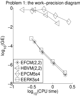
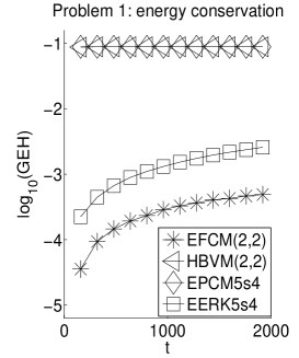
(i)	(ii)

Figure 1: Results for Problem 1. (i): The $\log$-$\log$ plot of the maximum global error ($GE$) over the integration interval against the execution time. (ii): The logarithm of the global error of Hamiltonian $GEH=|H_{n}-H_{0}|$ against $t$.

$$\begin{array}[]{|c|c|c|c|c|c|}\hline\cr\text{Methods}&tol=1.0e-006&tol=1.0e-008&tol=1.0e-010&tol=1.0e-012\\ \hline\cr\text{EFCM(2,2)}&2000&2000&2000&3000\cr\text{HBVM(2,2)}&2000&3000&3769&4000\cr\text{EPCM5s4}&2000&3000&4000&4999\cr\hline\cr\end{array}$$

Table 1: Results for Problem 1. The total numbers of iterations for different error tolerances (tol).

Problem 2. The Fermi–Pasta–Ulam problem is an important model for simulations in statistical mechanics which is considered in [14, 18, 19, 43, 46]. It is a Hamiltonian system with the Hamiltonian

$$H(x,y) =\dfrac{1}{2}\textstyle\sum\limits_{i=1}^{2m}y_{i}^{2}+\dfrac{\omega^{2}}{2}\textstyle\sum\limits_{i=1}^{m}x_{m+i}^{2}+\dfrac{1}{4}\Big{[}(x_{1}-x_{m+1})^{4}$$

$$+\textstyle\sum\limits_{i=1}^{m-1}(x_{i+1}-x_{m+i-1}-x_{i}-x_{m+i})^{4}+(x_{m}+x_{2m})^{4}\Big{]}.$$

This results in

$$\left(\begin{array}[]{c}x\\ y\\ \end{array}\right)^{\prime}+\left(\begin{array}[]{cc}\mathbf{0}_{2m\times 2m}&-I_{2m}\\ M&\mathbf{0}_{2m\times 2m}\end{array}\right)\left(\begin{array}[]{c}x\\ y\\ \end{array}\right)=\left(\begin{array}[]{c}0\\ -\nabla U(x)\\ \end{array}\right),\qquad t\in[0,t_{\textmd{end}}],$$ (32)

where

$$M=\left(\begin{array}[c]{cc}\mathbf{0}_{m\times m}&\mathbf{0}_{m\times m}\\ \mathbf{0}_{m\times m}&\omega^{2}I_{m\times m}\end{array}\right),$$

$$U(x)=\dfrac{1}{4}\Big{[}(x_{1}-x_{m+1})^{4}+\textstyle\sum\limits_{i=1}^{m-1}(x_{i+1}-x_{m+i-1}-x_{i}-x_{m+i})^{4}+(x_{m}+x_{2m})^{4}\Big{]}.$$

We choose

$$m=3,\ \omega=50,\ x_{1}(0)=1,\ y_{1}(0)=1,\ x_{4}(0)=\dfrac{1}{\omega},\ y_{4}(0)=1,$$

and choose zero for the remaining initial values. The system is integrated in the interval $[0,10]$ with the stepsizes $h=1/2^{k},\ k=3,4,5,6.$ We plot the work-precision diagram in Figure 2 (i). Then, we solve this problem in the interval $[0,1000]$ with the stepsize $h=1/10$ and present the energy conservation in Figure 2 (ii). Here, it is noted that we do not plot some points in Figure 2 when the errors of the corresponding numerical results are too large. Similar situation occurs in the next two problems. Furthermore, we solve the problem in $[0,10]$ with $h=0.01$ to show the convergence rate of iterations for the three implicit methods. Table 2 lists the total numbers of iterations for different error tolerances.

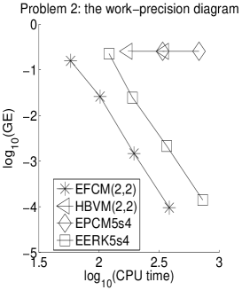
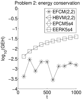
(i)	(ii)

Figure 2: Results for Problem 2. (i): The $\log$-$\log$ plot of the maximum global error ($GE$) over the integration interval against the execution time. (ii): The logarithm of the global error of Hamiltonian $GEH=|H_{n}-H_{0}|$ against $t$.

$$\begin{array}[]{|c|c|c|c|c|c|}\hline\cr\text{Methods}&tol=1.0e-006&tol=1.0e-008&tol=1.0e-010&tol=1.0e-012\\ \hline\cr\text{EFCM(2,2)}&2000&2080&2998&3027\cr\text{HBVM(2,2)}&6801&9291&10980&13912\cr\text{EPCM5s4}&9937&11925&14844&16945\cr\hline\cr\end{array}$$

Table 2: Results for Problem 2. The total numbers of iterations for different error tolerances (tol).

Problem 3. Consider the semilinear parabolic problem (this problem has been considered in [25])

$$\frac{\partial u}{\partial t}(x,t)=\dfrac{\partial^{2}u}{\partial x^{2}}(x,t)+\frac{1}{1+u(x,t)^{2}}+\Phi(x,t)$$

for $x\in[0,1]$ and $t\in[0,1],$ subject to homogeneous Dirichlet boundary conditions. The source function $\Phi(x,t)$ is chosen in such a way that the exact solution of the problem is $u(x,t)=x(1-x)\textmd{e}^{t}$.

We discretise this problem in space by using second-order symmetric differences with 1000 grid points. The problem is solved in the interval $[0,1]$ with different stepsizes $h=1/2^{i},\ i=2,3,4,5.$ The work-precision diagram is presented in Figure 3. Then, the problem is solved in $[0,1]$ with $h=\frac{1}{10}$ to show the convergence rate of iterations. See Table 3 for the total numbers of iterations for different error tolerances.

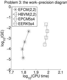
Figure 3: Results for Problem 3. The $\log$-$\log$ plot of the maximum global error ($GE$) over the integration interval against the execution time.

$$\begin{array}[]{|c|c|c|c|c|c|}\hline\cr\text{Methods}&tol=1.0e-006&tol=1.0e-008&tol=1.0e-010&tol=1.0e-012\\ \hline\cr\text{EFCM(2,2)}&40&50&60&73\cr\text{HBVM(2,2)}&86&86&86&86\cr\text{EPCM5s4}&87&87&87&87\cr\hline\cr\end{array}$$

Table 3: Results for Problem 3. The total numbers of iterations for different error tolerances (tol).

From the results, it can be clearly observed that the novel method EFCM(2,2) provides a considerably more accurate numerical solution than other methods and preserves well the Hamiltonian energy when solving Hamiltonian systems. Moreover, our method EFCM(2,2) requires less fixed-point iterations than both HBVM(2,2) and EPCM5s4, which is important in long-term computations.

6 Conclusions

In this paper, we formulated and analysed the novel methods EFCMs for solving systems of first-order differential equations. The novel EFCMs are an efficient kind of exponential integrators, and their construction takes full advantage of the variation-of-constants formula, the local Fourier expansion and collocation methods. We discussed the connections with HBVMs, Gauss methods, Radau IIA methods and TFCMs. It turned out that the first three traditional methods can be attained by letting $A\rightarrow 0$ in the corresponding EFCMs, and applying EFCMs to the second-order oscillatory differential equation (19) yields TFCMs. The properties of EFCMs were also analysed and it was shown that the new EFCMs can reach arbitrarily high order in a very convenient and simple way. A practical scheme of EFCMs was constructed in this paper. The numerical experiments were carried out and the results affirmatively demonstrate that the novel EFCMs have excellent numerical behaviour in comparison with some existing effective methods in the scientific literature.

This is a preliminary research on EFCMs for first-order ordinary differential equations and the authors are clearly aware that there are still some issues which will be further considered:

• The error bounds and convergence properties of EFCMs for linear and semilinear problems will be discussed in another work.

• For the EFCM(k,n) (15), it is assumed that $k\geq n$ in this paper. EFCMs with $k<n$ will be discussed and this case maybe not affect the computational cost associated with the implementation of the methods for some special systems. Some equations and unknowns in the methods may be removed and we will consider the efficient implementation of the novel EFCMs in a future research.

• We only consider the fixed-point iteration for the EFCMs in this paper. Other iteration methods such as waveform relaxation methods, Krylov subspace methods and preconditioning as well as their actual implementation for EFCMs will be analysed in future.

• The shifted Legendre polynomials are chosen as an orthonormal basis to give the Fourier expansion of the function $g(t,u(t))$. We observe that a different choice of the orthonormal basis would modify the arguments presented in this paper. The scheme of the numerical methods as well as their analysis is then modified accordingly. Different choices of the orthonormal basis will be considered in future investigations.

• Another issue for future exploration is the application of our methodology in other differential equations such as Schördinger equations and other stiff PDEs.

Acknowledgments. Bin Wang was supported by National Natural Science Foundation of China (Grant No. 11401333), by Natural Science Foundation of Shandong Province (Grant No. ZR2014AQ003) and by China Postdoctoral Science Foundation (Grant No. 2015M580578). Xinyuan Wu was supported by National Natural Science Foundation of China (Grant No. 11271186), by NSFC and RS International Exchanges Project (Grant No. 113111162), by Specialized Research Foundation for the Doctoral Program of Higher Education (Grant No. 20130091110041), by 985 Project at Nanjing University (Grant No. 9112020301), by A Project Funded by the Priority Academic Program Development of Jiangsu Higher Education Institutions. Fanwei Meng was supported by National Natural Science Foundation of China (Grant No. 11171178). Yonglei Fang was partially supported by National Natural Science Foundation of China (Grant No. 11571302) and the foundation of Scientific Research Project of Shandong Universities (Grant No. J14LI04).

References

• [1] A.H. Al-Mohy, N J. Higham, A new scaling and squaring algorithm for the matrix exponential, SIAM J. Mat. Anal. Appl. 31, 970-989 (2009).
• [2] A.H. Al-Mohy, N J. Higham, Computing the action of the matrix exponential, with an application to exponential integrators, SIAM J. Sci. Comput. 33, 488-511 (2011).
• [3] H. Berland, B. Owren, B. Skaflestad, B-series and order conditions for exponential integrators, SIAM J. Numer. Anal. 43, 1715-1727 (2005).
• [4] H. Berland, B. Skaflestad, W.M. Wright, EXPINT—A MATLAB package for exponential integrators, ACM Transactions on Mathematical Software (TOMS) 33, 4 (2007).
• [5] L. Brugnano, F. Iavernaro, C. Magherini, Efficient implementation of Radau collocation methods, Appl. Numer. Math. 87, 100-113 (2015).
• [6] L. Brugnano, F. Iavernaro, D. Trigiante, Hamiltonian boundary value methods (energy preserving discrete line integral methods), J. Numer. Anal. Ind. Appl. Math. 5, 17-37 (2010).
• [7] L. Brugnano, F. Iavernaro, D. Trigiante, A note on the efficient implementation of Hamiltonian BVMs, J. Comput. Appl. Math. 236, 375-383 (2011).
• [8] L. Brugnano, F. Iavernaro, D. Trigiante, A simple framework for the derivation and analysis of effective one-step methods for ODEs, Appl. Math. Comput. 218, 8475-8485 (2012).
• [9] L. Brugnano, F. Iavernaro, D. Trigiante, Energy and quadratic invariants preserving integrators based upon Gauss collocation formulae. SIAM J. Numer. Anal. 50, 2897-2916 (2012).
• [10] L. Brugnano, F. Mazzia, D. Trigiante, Fifty years of stiffness, Recent Advances in Computational and Applied Mathematics, Springer Netherlands 1-21 (2011).
• [11] M. Caliari, A. Ostermann, Implementation of exponential Rosenbrock-type integrators, Appl. Numer. Math. 59, 568-581 (2009).
• [12] M.P. Calvo, C. Palencia, A class of explicit multistep exponential integrators for semilinear problems, Numer. Math. 102, 367-381 (2006).
• [13] E. Celledoni, D. Cohen, B. Owren, Symmetric exponential integrators with an application to the cubic Schrödinger equation, Found. Comput. Math. 8, 303-317 (2008).
• [14] D. Cohen, T. Jahnke, K. Lorenz, C. Lubich, Numerical integrators for highly oscillatory Hamiltonian systems: a review, in Analysis, Modeling and Simulation of Multiscale Problems (A. Mielke, ed.), Springer, Berlin, 553-576 (2006).
• [15] S.M. Cox, P.C. Matthews, Exponential time differencing for stiff systems, J. Comput. Phys. 176, 430-455 (2002).
• [16] V. Grimm, M. Hochbruck, Error analysis of exponential integrators for oscillatory second-order differential equations, J. Phys. A: Math. Gen. 39, 5495-5507 (2006).
• [17] E. Hairer, Energy-preserving variant of collocation methods, JNAIAM J. Numer. Anal. Ind. Appl. Math. 5, 73–84 (2010).
• [18] E. Hairer, C. Lubich, Long-time energy conservation of numerical methods for oscillatory differential equations, SIAM J. Numer. Anal. 38, 414-441 (2000).
• [19] E. Hairer, C. Lubich, G. Wanner, Geometric Numerical Integration: Structure-Preserving Algorithms for Ordinary Differential Equations, 2nd edn. (Springer-Verlag, Berlin, Heidelberg, 2006).
• [20] E. Hairer, S.P. Nørsett, G. Wanner, Solving Ordinary Differential Equations II, Stiff and Differential-Algebraic Problems, (Springer-Verlag, Berlin, second edition, 1996).
• [21] J.K. Hale, Ordinary Differential Equations, (Roberte E. Krieger Publishing company, Huntington, New York, 1980).
• [22] N. J. Higham, A. H.Al-Mohy, Computing matrix functions, Acta Numer. 19, 159-208 (2010).
• [23] M. Hochbruck, C. Lubich, On Krylov subspace approximations to the matrix exponential operator, SIAM J. Numer. Anal. 34, 1911-1925 (1997).
• [24] M. Hochbruck, C. Lubich, H. Selhofer, Exponential integrators for large systems of differential equations, SIAM J. Sci. Comput. 19, 1552-1574 (1998).
• [25] M. Hochbruck, A. Ostermann, Explicit exponential Runge–Kutta methods for semilineal parabolic problems, SIAM J. Numer. Anal. 43, 1069-1090 (2005).
• [26] M. Hochbruck, A. Ostermann, Exponential Runge-Kutta methods for parabolic problems, Appl Numer Math 53, 323-339 (2005).
• [27] M. Hochbruck, A. Ostermann, Exponential integrators, Acta Numer. 19, 209-286 (2010).
• [28] M. Hochbruck, A. Ostermann, J. Schweitzer, Exponential rosenbrock-type methods, SIAM J. Numer. Anal. 47, 786-803 (2009).
• [29] F. Iavernaro, D. Trigiante, High-order symmetric schemes for the energy conservation of polynomial Hamiltonian problems, JNAIAM J. Numer. Anal. Ind. Appl. Math. 4, 787-101 (2009).
• [30] A. Iserles, On the global error of discretization methods for highly-oscillatory ordinary differential equations, BIT 42, 561-599 (2002).
• [31] A. Iserles, Think globally, act locally: solving highly-oscillatory ordinary differential equations, Appl. Num. Anal. 43, 145-160 (2002).
• [32] A.K. Kassam, L.N.Trefethen, Fourth-order time-stepping for stiff PDEs, SIAM J. Sci. Comput. 26, 1214-1233 (2005).
• [33] M. Khanamiryan, Quadrature methods for highly oscillatory linear and nonlinear systems of ordinary differential equations: part I, BIT Num. Math. 48, 743-762 (2008).
• [34] S. Krogstad, Generalized integrating factor methods for stiff PDEs, J. Comput. Phys. 203, 72-88 (2005).
• [35] C. Lubich, From quantum to classical molecular dynamics: reduced models and numerical analysis, (European Mathematical Society, 2008).
• [36] C. Moler, C. Van Loan, Nineteen dubious ways to compute the exponential of a matrix, twenty-five years later, SIAM review 45 3-49 (2003).
• [37] A. Ostermann, M. Thalhammer, W.M. Wright, A class of explicit exponential general linear methods, BIT Numer. Math. 46, 409-431 (2006).
• [38] L.N. Trefethen, Spectral methods in MATLAB, (SIAM, Philadelphia, 2000).
• [39] B. Wang, A. Iserles, Dirichlet series for dynamical systems of first-order ordinary differential equations, Disc. Cont. Dyn. Sys. B 19, 281-298 (2014).
• [40] B. Wang, A. Iserles, X. Wu, Arbitrary–order trigonometric Fourier collocation methods for multi-frequency oscillatory systems, Found. Comput. Math. 16, 151-181 (2016).
• [41] B. Wang, G. Li, Bounds on asymptotic-numerical solvers for ordinary differential equations with extrinsic oscillation, Appl. Math. Modell. 39, 2528-2538 (2015).
• [42] B. Wang, K. Liu, X. Wu, A Filon-type asymptotic approach to solving highly oscillatory second-order initial value problems, J. Comput. Phys. 243, 210-223 (2013).
• [43] B. Wang, X. Wu, A new high precision energy-preserving integrator for system of oscillatory second-order differential equations, Phys. Lett. A 376, 1185-1190 (2012).
• [44] B. Wang, X. Wu, Improved Filon-type asymptotic methods for highly oscillatory differential equations with multiple time scales, J. Comput. Phys. 276, 62-73 (2014).
• [45] X. Wu, B. Wang, W. Shi, Efficient energy-preserving integrators for oscillatory Hamiltonian systems, J. Comput. Phys. 235, 587-605 (2013).
• [46] X. Wu, B. Wang, J. Xia, Explicit symplectic multidimensional exponential fitting modified Runge-Kutta-Nyström methods, BIT 52, 773-795 (2012).
• [47] X. Wu, X. You, B. Wang, Structure-Preserving Algorithms for Oscillatory Differential Equations, (Springer-Verlag, Berlin, Heidelberg, 2013).