Multiple Infection Sources Identification with
Provable Guarantees

Abstract

Given an aftermath of a cascade in the network, i.e. a set $V_{I}$ of “infected” nodes after an epidemic outbreak or a propagation of rumors/worms/viruses, how can we infer the sources of the cascade? Answering this challenging question is critical for computer forensic, vulnerability analysis, and risk management. Despite recent interest towards this problem, most of existing works focus only on single source detection or simple network topologies, e.g. trees or grids.

In this paper, we propose a new approach to identify infection sources by searching for a seed set $S$ that minimizes the symmetric difference between the cascade from $S$ and $V_{I}$, the given set of infected nodes. Our major result is an approximation algorithm, called SISI, to identify infection sources without the prior knowledge on the number of source nodes. SISI, to our best knowledge, is the first algorithm with provable guarantee for the problem in general graphs. It returns a $\frac{2}{(1-\epsilon)^{2}}\Delta$-approximate solution with high probability, where $\Delta$ denotes the maximum number of nodes in $V_{I}$ that may infect a single node in the network. Our experiments on real-world networks show the superiority of our approach and SISI in detecting true source(s), boosting the F1-measure from few percents, for the state-of-the-art NETSLEUTH, to approximately 50%.

<ccs2012> <concept> <concept_id>10002951.10003227.10003351</concept_id> <concept_desc>Information systems Data mining</concept_desc> <concept_significance>500</concept_significance> </concept> <concept> <concept_id>10003752.10003809.10003635</concept_id> <concept_desc>Theory of computation Graph algorithms analysis</concept_desc> <concept_significance>500</concept_significance> </concept> <concept> <concept_id>10003752.10003809.10003636</concept_id> <concept_desc>Theory of computation Approximation algorithms analysis</concept_desc> <concept_significance>500</concept_significance> </concept> <concept> <concept_id>10002950.10003648.10003671</concept_id> <concept_desc>Mathematics of computing Probabilistic algorithms</concept_desc> <concept_significance>300</concept_significance> </concept> <concept> <concept_id>10002950.10003714.10003716.10011136.10011137</concept_id> <concept_desc>Mathematics of computing Network optimization</concept_desc> <concept_significance>300</concept_significance> </concept> <concept> <concept_id>10003033.10003083.10003095</concept_id> <concept_desc>Networks Network reliability</concept_desc> <concept_significance>300</concept_significance> </concept> <concept> <concept_id>10003033.10003106.10003114.10011730</concept_id> <concept_desc>Networks Online social networks</concept_desc> <concept_significance>300</concept_significance> </concept> </ccs2012>

[500]Theory of computation Graph algorithms analysis [500]Theory of computation Approximation algorithms analysis [300]Mathematics of computing Probabilistic algorithms [300]Mathematics of computing Network optimization [300]Networks Network reliability [300]Networks Online social networks

1 Introduction

The explosion of online social networks with billion of users such as Facebook or Twitter have fundamentally changed the landscapes of information sharing, nowadays. Unfortunately, the same channels can be exploited to spread rumors and misinformation that cause devastating effects such as widespread panic in the general public [1], diplomatic tensions [2], and witch hunts towards innocent people [3].

Given a snapshot of the network with a set $V_{I}$ of infected nodes who posted the rumors, identifying the set of nodes who initially spread the rumors is a challenging, yet important question, whether for forensic use or insights to prevent future epidemics. Other applications of infection source detection can be found in finding first computing devices that get infected with a virus or source(s) of contamination in water networks.

Despite recent interest towards this problem, termed Infection Sources Identifications (ISI), most of existing works either limit to single source detection [23, 22] or simple network topologies, e.g. trees or grids, with ad hoc extensions to general graphs [20, 26, 27, 23]. A recent work in [25] provides an MDL-based method, called NETSLEUTH, to detect both the number of infection sources and the sources themselves. However the proposed heuristics seems to only work well for grid networks and cannot detect any true infection source. Thus there is lack of a rigorous and accurate method to detect multiple infection sources in general graphs.

Figure 1: Infection sources detection on a $60\times 60$ grid graph

In this paper, we present a new approach to identify multiple infection sources that looks into both infected and uninfected nodes. This contradicts to existing methods [20, 25] which limit the attention to the subgraph induced by the infected nodes. Given a snapshot of network $G=(V,E)$ and a set of infected nodes $V_{I}$, we identify the sources by searching for a set $\hat{S}$ that minimize the symmetric difference between the cascade from $S$ and $V_{I}$. While our objective, the symmetric difference, is similar to the one used in $k$-effector [20], our novel formulation does not require the knowledge of the number of infection sources $k$. In deriving optimization method for this new approach, we face strong challenges in developing efficient solution:

• The exponential number, up to $2^{\theta(n)}$ for large $V_{I}$, of possible solutions. This makes the exhaustive search for the case of single source [23, 22, 12] intractable.

• The non-submodular objective. Thus, it is inefficient to solve the problem through simple greedy methods.

• The stochastic nature of the infection process requires considering exponentially many possible cascades.

To tackle ISI, we propose SISI, an algorithm that can accurately detect infection sources. We employ in SISI two novel techniques: a Truncated Reverse Infection Sampling (TRIS) method to generate random reachability RR sets that encode the infection landscape and a primal-dual algorithm for the Submodular-cost Covering [18]. SISI, to our best knowledge, is the first algorithm with provable guarantee for multiple infection sources detection in general graphs. It returns an $\frac{2}{(1-\epsilon)^{2}}\Delta$-approximate solution with a high probability, where $\Delta$ denotes the maximum number of nodes in $V_{I}$ that may infect the same node in the network. Experiments on real-world networks show the huge leap of SISI in detecting true infection sources, boosting the true source discovery rates from merely few percents, for the state-of-the-art NETSLEUTH, to more than 70%. Thus SISI has both high empirical performance and theoretical guarantees.

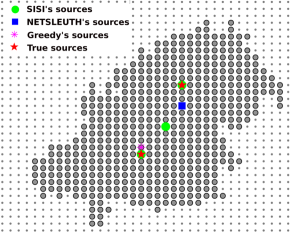
The advantages of SISI over other methods are illustrated through a cascade on a $60\times 60$ grid in Fig. 1. SISI is the only one which can detect the true infection sources. To avoid false negative, which is more serious than false positive, SISI often output slightly more infection sources than other methods (SISI: 3, NETSLEUTH: 1, Greedy:1, Ground-truth: 2). However, it maintains a reasonable F1-score of over 50%.

We summarize our contributions as follows

• We propose a new approach to identify multiple infection sources through minimizing the symmetric difference between the cascade of the suspected source nodes $S$ with the infected nodes $V_{I}$ without knowing the number of sources a priori. Our experiments show that methods following this approach including our algorithm SISI and the greedy algorithm outperform the other approaches in terms of detecting true sources.

• To our best knowledge, we propose the first approximation algorithm, termed SISI, for detecting multiple infection sources in general graphs and our algorithm does not require the knowledge on the number of infection sources. Given an approximation error $\epsilon>0$, we provide rigorous analysis on sample complexity, deriving the necessary number of samples to guarantee a multiplicative error $(1\pm\epsilon)$ on the objective estimation.

• Extensive experiments on real-world networks shows the superiority of SISI over other approaches in detecting the exact sources under both SI and IC models. The relax version of SISI is also faster than NETSLEUTH while still retaining high-quality solutions.

Related works. Infection Source Identification (ISI) under different names has recently emerged and attracted quite a number of researchers in multiple disciplines with diverse techniques. There are two main streams of works and methods that can be listed: 1) exact algorithms on tree graphs [26, 27, 23, 20, 11], 2) ad hoc heuristics approaches without any guarantee for general graphs [25, 23, 22].

In the first stream, Shah and Zaman in [26] established the notion of rumor-centrality which is an Maximum Likelihood estimator on regular trees under the SI model. They proposed an optimal algorithm to identify the single source of an epidemic. In [27], the same authors improved the previous results by deriving the exact expression for the probability of correct detection. Later Luo et al. [23] based on approximations of the infection sequences count to develop an algorithm that can find at most two sources in a geometric tree. Since solely targeting trees, all these methods are unable of solving ISI problem on general graphs.

Lappas et al. [20] formulated ISI problem under the name of $k$-effector and introduced the minimization of the symmetric difference between the observed infection and the resulting cascade if starting from a candidate source set. While the formulation is novel, their solution is, unfortunately, limited to tree graphs and require the knowledge of the number of infection sources. The extension for general graphs by approximating a graph by a tree does not work well either as we show later in the experiment section.

Prakash et al. [25] resort to heuristic approach to find multiple sources in general graphs and propose NETSLEUTH which relies on the two-part code Minimum Description Length. They show that NETSLEUTH is able to detect both the sources and how many of them. However, besides no guarantee on solution quality, we show in our experiments that NETSLEUTH performs poorly on a simple grid graph with large overlapping region of cascades from two source nodes. Luo et al. [23] also derived an estimator to find multiple sources given that the maximum number of sources is provided. Yet similar to [20], their estimator depends on the approximation of a general graph to tree and also requires the maximum number of sources.

There are also other works on related areas: [15] studies the rumor-centrality estimator on trees under an additional constraint that the status (infected or not) of a node is revealed with probability $p\leq 1$. In case of $p=1$, the estimator is able to reproduce the previous results and with large enough $p<1$, it achieves performance within $\epsilon$ the optimal. Under a different model, Chen et al. [9] study the problem of detecting multiple information sources in networks under the Susceptible-Infected-Recovered (SIR) model. They propose an estimator for regular trees that can detect sources within a constant distance to the real ones with high probability and investigate a heuristic algorithm for general cases. In another study [22], Lokhov et al. take the dynamic message-passing approach under SIR model and introduce an inference algorithm which is shown to admit good improvement.

Influence maximization problem [16] that find $k$ nodes to maximize the expected influence is one of the most extensively studied problem. The latest references on the problem can be found in [29] and the references therein.

Organization. We present our model and problem formulation in Section 2. The hardness and inapproximability results are provided in Section 2.3. The main algorithm SISI is proposed in Section 3 while its performance guarantees and running time are analyzed in Section 4. We provide comparison on empirical performance of our algorithms and other approaches in Section 5. Conclusions and extensions for other settings are discussed in Section 6.

2 Models and Problem definition

We represent the network in which the infection spreads as a directed graph $G=(V,E)$ where $V$ is the set of $n$ nodes, e.g., computers in a computer network, and $E$ is the set of $m$ directed edges, e.g., connections between the computers. In addition, we are given a subset $V_{I}\subseteq V$ of observed infected nodes and the remaining nodes are assumed to be not infected and denoted by $\bar{V_{I}}=V\backslash V_{I}$.

Table 1: Table of Notations

Notation	Description
$n,m$	#nodes, #edges of graph $G=(V,E)$.
$V_{I},\bar{V}_{I}$	Set of infected and uninfected nodes.
$\beta,k$	Infection probability and $k=|V_{I}|$.
$V(S,\mathcal{M})$	An infection cascade from $S$ under model $\mathcal{M}$.
$D(S,\mathcal{M},V_{I})$	Symmetric different on a graph realization.
$\mathbb{E}[D(S,\mathcal{M},V_{I})]$	The expectation of $D(S,\mathcal{M},V_{I})$ over all realizations.
$\hat{S}$	The returned source set of SISI.
$OPT,S^{*}$	The optimal value of $\mathbb{E}[D(S,\tau)]$ and an optimal solution set which achieves the optimal value.
$R_{j},\textsf{src}(R_{j})$	A random RR set and its source node $\textsf{src}(R_{j})$.
$\Delta$	Maximum size of an RR set ($\Delta\leq V_{I}$).
$c,M$	$c=2(e-2)\approx\sqrt{2}$, $M=2^{k}+1$.
$\Lambda$	$\Lambda=(1+\epsilon)2c(\ln\frac{2}{\delta}+k\ln 2+1)\frac{1}{\epsilon^{2}}$.

2.1 Infection Model

We focus on the popular Susceptible-Infected (SI) model.

Susceptible-Infected (SI) model. In this infection model, each node in the network is in one of two states: 1) Susceptible (S) (not yet infected) and 2) Infected (I) (infected and capable of spreading the disease/rumor). Once infected, the node starts spreading to its neighbors through their connections. While the initial model were proposed for a complete graph topology [5], the model can be extended for arbitrary graph $G=(V,E)$. We assume that the infection spreads in discrete time steps. At time $t=0$, a subset of nodes, called the infection sources, are infected and the rest is uninfected. Once a node $u$ gets infected at time $t$, it will continuously try to infect its uninfected neighbor $v$ and succeed with probability $0<\beta\leq 1$ from step $t+1$ onwards until successful. The single parameter $\beta$ indicates how contagious the infection is and thus the higher, the faster it contaminates the network.

Other cascade model. In principle, our formulation and proposed method will work for most progressive diffusion models in which once a node becomes infected, it stays infected. These include the two popular models Independent Cascade IC and Linear Threshold (LT) models [16]. Other non-progressive models can be first converted to a progressive ones as outlined in [8].

For simplicity, we present our method for the SI model and discuss the extension to the IC and LT models through changing the sampling method in Subsection 3.1.

Learning model parameters. Learning propagation model parameters is an important topic and has received a great amount of interest [17, 28, 14, 21, 19]. Our approaches can rely on these learning methods to extract influence cascade model parameters from real datasets, e.g., action logs, connection networks.

2.2 Problem Formulation

Intuitively, given an infection model, denoted by $\mathcal{M}$, the goal of infection source identification is to identify a set of source nodes $S$ (unknown size) so that the resulting cascade originated from nodes in $S$, within a duration $\tau>0$, matches $V_{I}$ as closely as possible.

To formalize the problem, we define a cascade $V(S,\mathcal{M})$ as the set of infected nodes if we select nodes in $S$ as the sources (initially infected) under infection model $\mathcal{M}$. Thus, the objective function which characterizes the aforementioned criteria, termed symmetric difference, is defined as follows,

$$D(S,\mathcal{M},V_{I})=|V_{I}\backslash V(S,\mathcal{M})|+|\bar{V_{I}}\cap V(S,\mathcal{M})|$$ (1)

Figure 2: Illustration of symmetric difference.

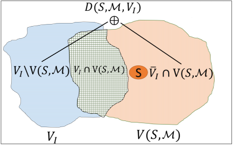
In Eq. 1, the first term $|V_{I}\backslash V(S,\mathcal{M})|$ counts the number of nodes in $V_{I}$ that are not infected by the propagation spreading from $S$ within a duration $\tau$ and the second term indicates the number of nodes that are “mistakenly” infected during the same time interval (illustrated in Fig. 2). Together, the sum measures the similarity between the observed cascade $V_{I}$ and the cascade causes by the suspected nodes $S$.

Due to the stochastic nature of the cascade, there are exponentially many possible cascades for a given set of source nodes $S$. Here cascade is used to refer to the set of infected nodes within $\tau$ steps. To account for this, we aggregate the symmetric difference over the probabilistic space of the possible cascades spreading from $S$. Denote by $\Pr[V(S,\mathcal{M})]$, the probability of receiving a particular cascade $V(S,\mathcal{M})$ within $t=\tau$ time steps. We compute the expected symmetric difference as follows,

$$\mathbb{E}[D(S,\mathcal{M},V_{I})]=\sum_{\text{possible }V(S,\mathcal{M})}D(S,\mathcal{M},V_{I})\Pr[V(S,\mathcal{M})]$$

$$=\sum_{\text{possible }V(S,\mathcal{M})}(|V_{I}\backslash V(S,\mathcal{M})|+|\bar{V_{I}}\cap V(S,\mathcal{M})|)\Pr[V(S,\mathcal{M})]$$

$$=\sum_{u\in V_{I}}\Pr[u\text{ not infected by }S]+\sum_{v\notin V_{I}}\Pr[v\text{ infected by }S]$$ (2)

In the last equation, the ‘infected’ and ‘not infected’ probabilities are w.r.t. a random cascade from $S$ within $\tau$ steps.

We now state the problem of identifying the infection sources as follows.

Definition 1 (Infection Sources Identification)

Given a graph $G=(V,E)$, infection model $\mathcal{M}$ (e.g., $\beta$ for SI model), observation set $V_{I}$ of infected nodes, and the duration of the cascade $\tau$ (could be infinity), the Infection Sources Identification (ISI) problem asks for a set $\hat{S}$ of nodes such that,

$$\hat{S}=\arg\min_{S\subseteq V_{I}}\mathbb{E}[D(S,\mathcal{M},V_{I})]$$ (3)

While this formulation is similar to [20], we do not require knowledge on the number of infection sources.

2.3 Hardness and Inapproximability

This subsection shows the NP-hardness and inapproximability results of the ISI problem. From Def. 1, there are two major difficulties in finding the sources: 1) first, by a similar argument to that of the influence maximization problem in [16], the objective function is #P-hard to compute exactly; 2) second, the objective is non-submodular, i.e., there are no easy greedy approaches to obtain approximation algorithms. In fact, we show a stronger inapproximability result in the below theorem.

Theorem 1

ISI cannot be approximated within a factor $O(2^{\log^{1-\epsilon}n})$ for any $\epsilon>0$, where $n=|V|$, unless NP $\subseteq$ DTIME($n^{polylog(n)}$).

Proof 2.2.

To prove Theo. 1, we construct a gap-preserving polynomial-time reduction which reduces any instance of the Red-Blue Set Cover problem [7] to an instance of ISI. The Red-Blue Set Cover problem is defined as follows: an instance of Red-Blue Set Cover problem consists of two disjoint sets: $R=\{r_{1},...,r_{p}\}$ of red elements, $B=\{b_{1},...,b_{q}\}$ of blue elements, and a family $T\subseteq 2^{R\cup B}$ of $n(n\geq p,n\geq q)$ subsets of $R\cup B$. The problem asks a subfamily $C^{*}\subseteq T$ of subsets that covers all the blue elements but minimum number of reds,

$$C^{*}=\arg\min_{C\subseteq T}\{|R\cap(\cup_{i=1}^{|C|}T_{i})|\}$$ (4)

Our polynomial reduction ensures that if the ISI instance has an $O(2^{\log^{1-\epsilon}n})$-approximate solution $S$, then there must be a corresponding $O(2^{\log^{1-\epsilon}n})$-approximate solution of the Red-Blue Set Cover polynomially induced from $S$. The reduction is grounded on the observation that any solution of the Red-Blue Set Cover costs at most $p$ - the number of red elements. Then, based on the result in [7] that the Red-Blue Set Cover cannot be approximated within a factor $O(2^{\log^{1-\epsilon}N})$ where $N=n^{4}$ for any $\epsilon>0$ unless NP $\subseteq$ DTIME($N^{polylog(N)}$), we obtain the Theorem 1.

We will give a polynomial reduction from an instance of the Red-Blue Set Cover to an ISI instance with $\beta=1$ and $\tau=1$ such that,

• The optimal solution of the ISI instance polynomially infers the optimal solution for the instance of Red-Blue Set Cover.

• If we obtain an $O(2^{\log^{1-\epsilon}n})$-approximate solution for ISI, we will also have an $O(2^{\log^{1-\epsilon}n})$-approximate solution for the Red-Blue Set Cover instance.

These two conditions are sufficient to conclude that we cannot approximate the optimal solution of ISI within a factor $O(2^{\log^{1-\epsilon}n})$ unless we can do that for Red-Blue Set Cover. Thus, the Theorem 1 follows. We will present the reduction and then prove the satisfaction of each condition.

Figure 3: Reduction from Red-Blue Set Cover to ISI in which infected nodes are blue-colored and uninfected nodes are in red.

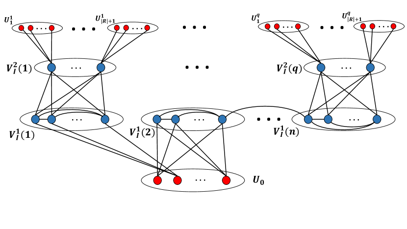
Given an instance of Red-Blue Set Cover with two sets $R,B$ and a family $T$, we suppose all the subsets in $T$ contains at least a blue element, otherwise we can trivially discard all those subsets since we never select that type of subsets. In the reverse way, we also suppose every pair of subset in $T$ has at least one red element different from each other. Otherwise we always select/reject both at the same time without changing the cost, in other words, we can group together to create one subset. We construct a corresponding ISI instance consisting of the node set $V$, the infected set $V_{I}\subseteq V$ and the set of edges $E$ as follows (depicted in Fig. 3):

• Set of infected nodes $V_{I}$: For each subset $T_{i}\in T$, there is a set $V_{I}^{1}(i)$ of infected nodes whose number is the number of blues in $T_{i}$. For each blue node $B_{j}$ in $B$, we form a set $V_{I}^{2}(j)$ of $|R|+1$ infected nodes.

• Set of uninfected nodes $V\backslash V_{I}$: For each infected node $l$ in $V_{I}^{2}(j)$, a set $U_{l}^{j}$ of $|R|+1$ uninfected nodes is constructed. We also have a set $U_{0}$ of $p$ uninfected nodes corresponding to the red set $R$ in Red-Blue Set Cover instance.

• Set of edges $E$: For any pair $(u,v)\in V_{I}^{1}(i)$, we connect them by an edge, so that the subgraph of nodes in $V_{I}^{1}(i)$ is a clique. For each $u\in T_{i}\cap T_{j}$, we connect the two corresponding nodes in $V_{I}^{1}(i)$ and $V_{I}^{1}(j)$ by an edge. For each $u\in V_{I}^{1}(i)$, we connect $u$ to all $|R|+1$ nodes in $V_{I}^{2}(u)$ and, subsequently, each node $l$ in $V_{I}^{2}(u)$ is connected to all $|R|+1$ nodes in $U_{l}^{u}$. For any pair $u,v\in V_{I}^{1}(j)$ for each $j\in\{1,...,n\}$, we connect $u$ with all the nodes in $V_{I}^{2}(v)$ and $v$ with all the nodes in $V_{I}^{2}(u)$. If the subset $T_{i}$ contains red element $R_{j}$, then for each $u\in V_{I}^{1}(i)$, there is an edge connecting $u$ to the corresponding node of $R_{j}$ in $U_{0}$.

Now, we will prove the two conditions consecutively. Our proof relies on two observations: the first one is that if the feasible solution for ISI contains at least an infected node from $V_{I}^{2}(j)$ for some $j\in\{1,...,q\}$, then the number of uninfected nodes covered is at least $|R|+1$ which causes the cost to be at least $|R|+1$. The same phenomenon happens if an infected node $v$ in $V_{I}^{1}(j)$ for some $j\in\{1,...,n\}$ is not covered since there would be $|R|+1$ infected nodes in $V_{I}^{2}(v)$ not covered. On the other hand, if all the infected nodes in $V_{I}^{1}(j)$ for all $j\in\{1,...,n\}$ are covered, then all infected nodes in the whole network are indeed covered and at most $|R|$ uninfected nodes (in $U_{0}$) are also covered. The second observation with the previous case is that in the original Red-Blue Set Cover instance, we select those subset $T_{i}$ such that the corresponding $V_{I}^{1}(i)$ contains a infection source chosen in ISI, then the cost in the two problem are equal (cover the same number of red elements/uninfected nodes).

Prove condition (1). Based on our observation, the optimal solution $S^{*}$ of the ISI instance has to cover all the nodes in $V_{I}^{1}(j)$ for all $j$ and has the least number of uninfected nodes covered. From this solution, we construct the solution for the original Red-Blue Set Cover instance by selecting the subfamily $C^{*}$ of subsets $T_{i}$ such that the corresponding $V_{I}^{1}(i)$ contains a infection source in the optimal solution of ISI. First, this subfamily covers all the blue elements since each blue element corresponds to some infected nodes in $V_{I}^{1}(j)$ for some $j$. Secondly, if this subfamily has the lowest cost (covers the least number of red elements). Otherwise, suppose that a different subfamily $\hat{C}$ has lower cost, then we can equivalently find another solution for the reduced ISI instance and obtain the same cost (lower than that of $S^{*}$). That contradicts with the optimality of $S^{*}$.

Prove condition (2). Based on condition (1) that the optimal solution of ISI instance infers the optimal solution of Ref-Blue Set Cover with the same cost. Suppose we have an $O(2^{\log^{1-\epsilon}n})$-approximate solution $\hat{S}$ for Red-Blue Set Cover instance, there are two possible cases:

• If $\hat{S}$ contains a node in $V_{I}^{2}(j)$ for some $j$ or $\hat{S}$ does not cover a node in $V_{I}^{1}(j)$ for some $j$, then based on the first observation, the cost of $\hat{S}$ has to be at least $|R|+1$. Because this is an $O(2^{\log^{1-\epsilon}n})$-approximate solution, we just select the whole family $T$ in Red-Blue Set Cover instance which has cost of only $|R|$ and obtain an $O(2^{\log^{1-\epsilon}n})$-approximate solution.

• Otherwise, based on the second observation, we can easily construct a solution for Red-Blue Set Cover with equal cost and thus obtain an $O(2^{\log^{1-\epsilon}n})$-approximate solution.

Lastly, note that the number of blue and red elements must be at least $|T|$, otherwise we can drop or merge some sets together without effecting any solution. Thus, by following our construction of the ISI instance, we determine the number of uninfected nodes,

$$|V| =|U_{0}|+\sum_{i=1}^{n}|V_{I}^{1}(i)|+\sum_{i=1}^{q}|V_{I}^{2}(i)|\cdot\sum_{j=1}^{|R+1|}|U^{i}_{j}|$$

$$\leq|T|+|T|+|T|^{2}(|T|+1)\leq|T|^{4}\text{ \ \ \ }(\text{|}T|\geq 4)$$ (5)

Since $|T|=n$ and the Red-Blue Set Cover cannot be approximated within a factor of $O(2^{\log^{1-\epsilon}N})$ where $N=n^{4}$ for any $\epsilon>0$ unless NP $\subseteq$ DTIME($N^{polylog(N)}$), we obtain our results in Theo. 1.

3 Sampling-based SISI algorithm

In this section, we present SISI, our sampling-based method with guarantee on achieving $\frac{2}{(1-\epsilon)^{2}}\Delta$-approximation factor for arbitrary small $\epsilon>0$. Here $\Delta$ equals the maximum nodes in $V_{I}$ that can infect a single node in the graph and is the same with the maximum sample size in Subsec. 3.1.

Outline. SISI contains two key components: 1) an efficient Truncated Reverse Infection Sampling (TRIS) to compute the objective with high accuracy and confidentiality (presented in Subsection 3.1) and 2) an innovative transformation of the studied problem into a submodular-cost covering problem to provide high quality solutions with performance guarantees (presented in Subsection 3.2). We show the combination of the two components to obtains the SISI algorithm in Subsection 3.3.

3.1 Truncated Reverse Infection Sampling

We propose the Truncated Reverse Infection Sampling (TRIS) strategy to generate random Reverse Reachable (RR) sets, following the reverse influence sampling method (RIS) pioneered in [6]. A RR set, $R_{j}$, is generated as follows.

Definition 2 (Reverse Reachable set (RR set))

Given $G=(V,E)$, probability $\beta$ and propagation time $\tau$, a RR set is generated from $G$ by 1) selecting a (uniformly) random source node $v\in V$, 2) generating a reverse random cascade from $v$ in $G$ within $\tau$ steps and 3) returning $R_{j}$ as the set of nodes in the cascade.

The main intuition is that each RR set $R_{j}$ contains the nodes that can infect its source $v=\textsf{src}(R_{j})$ within a given time $\tau$. Thus RR sets were used in previous works [6, 29, 24] (without the step/time limit $t$) to estimate influence of nodes. We shall show later in next subsection that RR sets can also be fine-tuned to estimate the chance of being infection sources.

Note that the above description of generating RR sets is model-independent, i.e., you can use it with many different cascade models for reverse cascade simulation in the step 2. For example, the reverse simulation for IC and LT, the two most popular cascades models, are presented in [6] and [4], respectively. Here we focus on the reverse sampling for SI model and highlight the necessary changes to make the method work for our problem.

Input: Graph $G$, probability $\beta$, max time $\tau$ and $V_{I}$

Output: A random RR set $R_{j}$

1 Pick a random node $u\in V$

2 RR set $R_{j}=\{u\}$

3 Infection time $T\{v\}=\infty$, $\forall v\in V\backslash\{u\}$, $T\{u\}=0$

4 Min priority queue $PQ=\{u\}$

5 while $PQ$ not empty do

6       $u=PQ.pop()$

7       foreach  $v\in(\text{in-neighbors}(u)\backslash R_{j})\cup PQ$ do

8             $r\leftarrow$ a random number in [0,1]

9             $t\leftarrow\lceil\log_{1-\beta}(1-r)\rceil$ {Assume $0<\beta<1$}

10             $T(v)=\min\{T(v),T(u)+t\}$

11             if $T(v)<\tau$ then

12                   if $v\notin R_{j}$ then

13                         if $v\in V_{I}$ then

14                               $R_{j}=R_{j}\cup\{v\}$

15                              

16                        $PQ.push(v)$

17                        

18                  else

19                         $PQ.update(v)$

20                        

21                  

22            

23      

24Return $R_{j}$

Algorithm 1 Fast-TRIS

3.1.1 Generating RR Sets under SI model.

The main difference between SI model vs. LT and IC models are SI model allows multiple attempts for an infected node to its neighbors in contrast to a single attempt in IC and LT. Given a network $G=(V,E)$ and infection probability $0<\beta\leq 1$, RR sets in the SI model are generated as follows.

• Select a random node $u$. Only $u$ is infected at time $0$ and all other nodes are not infected.

• For each time step $i\in[1,\tau]$, consider all edges $(u,v)\in E$ in which $v$ is infected and $u$ is not infected (note the direction). Toss a $\beta$-head biased coin to determine whether $u$ succeeds in infecting $v$. If the coin gives head (with a probability $\beta$), we mark $u$ as infected.

• After $\tau$ steps, return $R_{j}$ as the set of infected nodes, removing all nodes that are not in $V_{I}$.

Note the last step, the nodes that are not in $V_{I}$ will be removed from the RR set (hence the name truncated). This truncation is due to the observation that the suspected nodes must be among the infected nodes in $V_{I}$. Our RR sets are in general smaller than the RR sets in [6] and might be empty. This saves us a considerable amount of memory in storing the RR sets.

A naive implementation of the above reserve sampling has a high complexity and does not scale when $\tau$ grows, thus we present a fast implementation using geometric distribution in Algorithm 1.

The complete pseudocode for the fast TRIS algorithm is described in Alg. 1. The key observation to speed up the TRIS procedure is that each trial in the sequence of infection attempts is a Bernoulli experiment with success probability of $\beta$. Thus this sequence of attempts until successful actually follows a geometric distribution. Instead of tossing the Bernoulli coin many times until getting a head, we can toss once and use the geometric distribution to determine the number of Bernoulli trials until successful (Lines 8,9).

Another issue is the order of attempts since a node can be infected from any of her in-neighbors but only the earliest one counts. Therefore, we will keep the list of all newly infected nodes in a min priority queue (PQ) w.r.t infection time. In each iteration, the top node is considered (Lines 6). The algorithm behaves mostly like the legacy Dijkstra’s algorithm [13] except we have time for a node $w$ to infect a node $v$ on each edge $(w,v)$ instead of the length. Also, the algorithm is constrained within the region consisting of nodes at most ‘distance’ $\tau$ from the selected $u$.

The time complexities of the naive and fast implementation of TRIS are stated in the following lemma.

Lemma 1

Expected time complexity of the naive TRIS is,

$$C(R_{j})=\frac{\Delta m\tau}{n}$$ (6)

and that of the fast implementation is,

$$C^{\prime}(R_{j})=\frac{\Delta m}{n}+\Delta\log(\Delta)\log(1+\frac{\Delta m}{n^{2}})$$ (7)

Proof 3.3.

Similar to the analysis of Expected Performance of Dijkstra’s Shortest Path Algorithm in [13] and denote the expected complexity of the fast algorithm by $C^{\prime}(R_{j})$, we have,

$$C^{\prime}(R_{j})=C(edges)+\Delta\log(\Delta)\log(1+C(edges)/n)$$ (8)

where $C(edges)$ is the expected number of edges examined. Note that this is different from $C(R_{j})$ since in this case, each edge can be checked once while, for the latter, it is multiple until successful. $\Delta$ is defined previously as the maximum size of a RR set. We also have,

$$C(edges)\leq\frac{1}{n}\sum_{u\in V}\sum_{v\in V}\Pr[u,v]d^{in}(v)\leq\frac{\Delta m}{n}$$ (9)

in which the details are similar to that of Eq. 6. Thus, combining with Eq. 8, we obtain,

$$C^{\prime}(R_{j})=\frac{\Delta m}{n}+\Delta\log(\Delta)\log(1+\frac{\Delta m}{n^{2}})$$ (10)

In Eq. 7, the first term is usually the leading factor and, then, the complexity depends mostly on $\frac{\Delta m}{n}$. We now analyze the expected time complexity $C(R_{j})$ of generating $R_{j}$ by the naive way.

$$C(R_{j})\leq\frac{\tau}{n}\sum_{u\in V}\sum_{v\in V}\Pr[u,v]d^{in}(v)=\frac{\tau}{n}\sum_{v\in V}d^{in}(v)\sum_{u\in V}\Pr[u,v]$$

where $\Pr[u,v]$ is the probability of $v$ infected by $u$ within $\tau$ steps, $d^{in}(v)$ is the in-degree of $v$. Here we take the average over all possible sources $u$ of $R_{j}$ (each has probability $1/n$) and the maximum number of edge checks for node $v$ is $\tau d^{in}(v)$. Let denote the maximum size of a random RR set as $\Delta$, we get $\sum_{u\in V}\Pr[u,v]\leq\Delta$ and thus,

$$C(R_{j})\leq\frac{\tau}{n}\sum_{v\in V}d^{in}(v)\Delta=\frac{\Delta\tau}{n}\sum_{v\in V}d^{in}(v)=\frac{\Delta m\tau}{n}$$ (11)

From Eq. 6, the complexity depends linearly on $\tau$ and is very high with large values of $\tau$.

Thus, the running time $C^{\prime}(R_{j})$ of our fast implementation is roughly $\tau$ times smaller than that $C(R_{j})$ of the naive implementation, especially, for large values of $\tau$.

3.1.2 Chance of Being Infection Sources

We show how to utilize the generated RR sets to estimate the chance that nodes being infection sources. First, we classify each generated RR $R_{j}$ into one of the two groups, based on the source of $R_{j}$, denoted by $\textsf{src}(R_{j})$.

• $\mathcal{R}_{Blue}=\{R_{j}|\textsf{src}(R_{j})\in V_{I}\}$: The set of blue RR sets that sources are.

• $\mathcal{R}_{Red}=\{R_{j}|\textsf{src}(R_{j})\notin V_{I}\}$: The set of red RR sets that sources are not in $V_{I}$.

Since the infection sources infect the nodes in $V_{I}$ but not the nodes outside of $V_{I}$ (within a time $\tau$), thus, the infection sources should appear frequently in blue RR sets (of which sources are in $V_{I}$) and appear infrequently in red RR sets (of which sources are not in $V_{I}$.) Thus, a node $v$ that appear in many blue RR and few red RR sets will be more likely to be among the infection sources.

The above observation can be generalized for a given a subset of nodes $S\subset V_{I}$, e.g., a subset of suspected nodes. A subset $S$ that covers (i.e. to intersect with) many blue RR sets and few red RR sets will be more likely to be the infection sources.

Define the following two subgroups of RR sets,

$$\mathcal{R}_{Blue}^{-}(S) =\{R_{j}|R_{j}\in\mathcal{R}_{Blue}\text{ and }R_{j}\cap S\mathbb{=}\emptyset\},\text{ and }$$ (12)

$$\mathcal{R}_{Red}^{+}(S) =\{R_{j}|R_{j}\in\mathcal{R}_{Red}\text{ and }R_{j}\cap S\mathbb{\neq}\emptyset\}.$$ (13)

They are the blue RR sets that a suspected subset $S$ “fails” to cover (i.e. to intersect with) and the red RR sets that $S$ (“mistakenly”) covers. The less frequent a random RR set $R_{j}$ falls into one of those two subgroups, the more likely $S$ will be the infection sources.

Formally, we can prove that the probability of a random RR set falls into one of those two subgroups equals exactly our objective function, denoted by $\mathbb{E}[D(\hat{S},\tau,V_{I})]$. We state the result in the following lemma.

Lemma 2

Given a fixed set $S\in V_{I}$, for a random RR set $R_{j}$, denote $X_{j}$ a random variable such that,

$$X_{j}=\left\{\begin{array}[]{ll}1&\mbox{if }R_{j}\in\mathcal{R}^{-}_{Blue}(S)\text{ or }R_{j}\in\mathcal{R}^{+}_{Red}(S)\\ 0&\mbox{otherwise}\end{array}\right.$$ (16)

then,

$$\mathbb{E}[X_{j}]=\frac{\mathbb{E}[D(S,\tau,V_{I})]}{n}$$ (17)

Proof 3.4.

Since for a random RR set $R_{j}$, $R_{j}\in\mathcal{R}^{-}_{Blue}(S)$ and $R_{j}\in\mathcal{R}^{+}_{Red}(S)$ are two mutually exclusive events,

$$\mathbb{E}[X_{j}]= \Pr_{R_{j}}[R_{j}\in\mathcal{R}^{-}_{Blue}(S)]+\Pr_{R_{j}}[R_{j}\in\mathcal{R}^{+}_{Red}(S)]$$ (18)

We will prove an equivalent formula of Eq. 17 that,

$$\mathbb{E}[D(S,\tau)]=n(\Pr_{R_{j}}[R_{j}\in\mathcal{R}^{-}_{Blue}(S)]+\Pr_{R_{j}}[R_{j}\in\mathcal{R}^{+}_{Red}(S)])$$

Let define $\mathcal{G}$ as a realization of the graph $G$, $\mathcal{G}\sim G$, where each edge $(u,v)$ is assigned a length value indicating the number of trials $u$ has to make until $v$ gets infected from $u$. In one realization $\mathcal{G}$, the cascade from $S$ at time $\tau$, $V(S,\tau)$, is uniquely defined (the reachable nodes from $S$ within $\tau$-length path) and so as $D(S,\tau)$. According to the definition of $\mathbb{E}[D(S,\tau)]$ in Eq. 2, we have,

$$\mathbb{E}[D(S,\tau)]=\sum_{u\in V_{I}}\Pr_{\mathcal{G}\sim G}[u\text{ not infected}]+\sum_{v\notin V_{I}}\Pr_{\mathcal{G}\sim G}[v\text{ infected}]$$

Let denote $R_{j}(u)$ be a random RR set rooted at $u$, the first term in the right-hand side is equivalent to,

$$\sum_{u\in V_{I}}\Pr_{\mathcal{G}\sim G}[u\text{ not infected}]=\sum_{u\in V_{I}}\Pr_{R_{j}(u)\vdash\mathcal{G}}[S\cap R_{j}(u)=\emptyset]$$

where $R_{j}(u)\vdash\mathcal{G}$ denotes the consistency of $R_{j}(u)$ to $\mathcal{G}$ since $\mathcal{G}$ is a realization of $G$ and thus $R_{j}(u)$ is well-defined. Since,

$$\Pr_{R_{j}(u)\vdash\mathcal{G}}[S\cap R_{j}(u)=\emptyset]=\Pr_{R_{j}}[S\cap R_{j}=\emptyset\text{ }|\text{ }\textsf{src}(R_{j})=u]$$

we obtain,

$$\sum_{u\in V_{I}} \Pr_{\mathcal{G}\sim G}[u\text{ not infected}]=\sum_{u\in V_{I}}\Pr_{R_{j}}[S\cap R_{j}=\emptyset\text{ }|\text{ }\textsf{src}(R_{j})=u]$$

$$=\sum_{u\in V_{I}}\frac{\Pr_{R_{j}}[S\cap R_{j}=\emptyset\text{ }\&\text{ }\textsf{src}(R_{j})=u]}{\Pr_{R_{j}}[\textsf{src}(R_{j})=u]}$$

$$=\sum_{u\in V_{I}}\Pr_{R_{j}}[S\cap R_{j}=\emptyset\text{ }\&\text{ }\textsf{src}(R_{j})=u]\cdot n$$

(since the source of each RR set is randomly chosen)

$$=n\sum_{u\in V_{I}}\Pr_{R_{j}}[S\cap R_{j}=\emptyset\text{ }\&\text{ }\textsf{src}(R_{j})=u]$$

$$=n\Pr_{R_{j}}[S\cap R_{j}=\emptyset\text{ }\&\text{ }\textsf{src}(R_{j})\in V_{I}]$$ (19)

$$=n\Pr_{R_{j}}[R_{j}\in\mathcal{R}^{-}_{Blue}(S)]$$ (20)

The Eq. 19 follows from the fact that, for all $u\in V_{I}$, $(S\cap R_{j}=\emptyset\text{ }\&\text{ }\textsf{src}(R_{j})=u)$ are mutually exclusive. Thus,

$$\sum_{u\in V_{I}}\Pr_{\mathcal{G}\sim G}[u\text{ not infected}]=n\Pr_{R_{j}}[R_{j}\in\mathcal{R}^{-}_{Blue}(S)]$$ (21)

Similarly, we can also achieve,

$$\sum_{v\in\bar{V}_{I}}\Pr_{\mathcal{G}\sim G}[v\text{ infected}]=n\Pr_{R_{j}}[R_{j}\in\mathcal{R}^{+}_{Red}(S)]$$ (22)

From Eq. 21, Eq. 22 and Eq. 18, we obtain

$$\mathbb{E}[D(S,\tau)]=n(\Pr_{R_{j}}[R_{j}\in\mathcal{R}^{-}_{Blue}(S)]+\Pr_{R_{j}}[R_{j}\in\mathcal{R}^{+}_{Red}(S)])$$

which completes the proof of Lem. 2.

Lem. 2 suggests a two-stages approach to identify the infection sources: 1) generating many RR sets and 2) look for a subset $S\subset V_{I}$ that minimize the size of $|\mathcal{R}^{-}_{Blue}(S)\cup R_{j}\in\mathcal{R}^{+}_{Red}(S)|$. In next two subsections, we address two key issues of this approach 1) Optimization method to identify $S$ with guarantees and 2) Sample complexity, i.e., how many RR sets is sufficient to generate a good solution. Too few RR sets lead to biased and poor solutions, while too many RR set lead to high running time.

3.2 Submodular-cost Covering

We will transform the ISI problem to a submodular-cost covering problem over the generated RR sets. This allows us to apply the $\Delta$-approximation algorithm in [18], where $\Delta$ is the maximum size of any RR set.

By Lemma 2, the problem of minimizing $\mathbb{E}[D(S,\mathcal{M},V_{I})]$ can be cast as a minimization problem of $\Pr[R_{j}\in\mathcal{R}^{-}_{Blue}(S)\cup\mathcal{R}^{+}_{Red}(S)]$. This, in turn, can be approximated with the following problem over the generated RR sets.

$$\min_{S\subseteq V_{I}}|\mathcal{R}^{-}_{Blue}(S)\cup\mathcal{R}^{+}_{Red}(S)|,$$ (23)

and, since $R_{j}\in\mathcal{R}^{-}_{Blue}(S)$ and $R_{j}\in\mathcal{R}^{+}_{Red}(S)$ are disjoint, the above minimization problem is equivalent to,

$$\min_{S\subseteq V_{I}}|\mathcal{R}^{-}_{Blue}(S)|+|\mathcal{R}^{+}_{Red}(S)|$$ (24)

We shall convert the above problem to the submodular-cost covering in [18], stated as follows.

Definition 3 (Submodular-cost covering)

[18] An instance is a triple $(c,\mathcal{C},U)$ where

• The cost function $c(x):\mathbf{R}^{n}_{\geq 0}\rightarrow\mathbf{R}_{\geq 0}$ is submodular, continuous, and non-decreasing.

• The constraint set $\mathcal{C}\subseteq 2^{\mathbf{R}_{\geq 0}}$ is a collection of covering constraints, where each constraint $S\in\mathcal{C}$ is a subset of $\mathbf{R}^{n}_{\geq 0}$.

• For each $j\in[n]$, the domain $U_{j}$ for variable $x_{j}$ is any subset of $\mathbf{R}_{\geq 0}$.

The problem is to find $x\in\mathbf{R}^{n}_{\geq 0}$, minimizing $c(x)$ subject to $x_{j}\in U_{j},\forall j\in[n]$ and $x\in S,\forall S\in\mathcal{C}$.

Figure 4: Conversion to Submodular-cost covering.

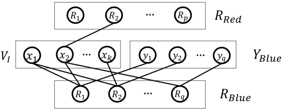
Conversion to submodular-cost covering problem. We convert the form in Eq. 24 into a submodular-cost covering problem as demonstrated in Fig. 4. Let $q=|\mathcal{R}_{Blue}|$ and $p=|\mathcal{R}_{Red}|$. We associate a variable $x_{u}\in[0,1]$ for each $u\in V_{I}$ to indicate whether the corresponding node is selected as an infected source. We also assign a variable $y_{j}$ to each RR set $R_{j}\in\mathcal{R}_{Blue}$. We require all blue RR $R_{j}$ sets to be covered through the constraint $\max\{\max_{u\in R_{j}}x_{u},y_{j}\}\geq 1$. Thus for each blue $R_{j}$ either $x_{v}=1$ for some $v\in R_{j}$ or the corresponding $y_{j}=1$.

The objective is to minimize the cost function $\min_{x,y}c(x,y)=\sum_{R_{j}\in\mathcal{R}_{Red}}\max_{u\in R_{j}}(x_{u})+\sum_{j=1}^{q}y_{j}$. The first part of the cost function $\max_{u\in R_{j}}(x_{u})$ is a submodular function since the $\max$ function is submodular (see footnote 1, page 2 in [18]). The second part $\sum_{j=1}^{q}y_{j}$ is a linear function, and thus is also a submodular function. Therefore, the objective is a submodular function.

Thus, the problem in Eq. 24 can be converted to the following submodular-cost covering problem,

$$\quad\quad\min_{x,y}c(x,y)=\sum_{R_{j}\in\mathcal{R}_{Red}}\max_{u\in R_{j}}(x_{u})+\sum_{j=1}^{q}y_{j}$$ (25)

$$\text{subject to (for each }R_{j}\in\mathcal{R}_{Blue}\text{) }\max\{\max_{u\in R_{j}}x_{u},y_{j}\}\geq 1$$

Since for any assignment of variable set $x$, we have a corresponding source selection: node $u$ is selected as infection source if $x_{u}=1$. The first term $\sum_{R_{j}\in\mathcal{R}_{Red}}\max_{u\in R_{j}}(x_{u})$ in Eq. 25 is equivalent to $|\mathcal{R}^{+}_{Red}(S)|$ in Eq. 24 and similarly $\sum_{j=1}^{q}y_{j}$ together with the constraints is equivalent to $|\mathcal{R}^{-}_{Blue}(S)|$. In Eq. 25, each covering constraint is associated with a blue RR set $R_{j}$ and says that if $R_{j}$ is not covered by any variable $x_{u}$ ($x_{u}=1$), then $y_{j}=1$ which will increase the cost function by 1. Thus, Eq. 25 minimizes the number of red RR sets covered and blue RR sets uncovered.

Input: Infected set $V_{I}$, collection of RR sets $\mathcal{R}$

Output: An $\Delta$-approximate set $\hat{S}$

1 Formulate the submodular cost covering version from $\mathcal{R}$

2 $x_{u}=0,\forall u\in V_{I}$ and $y_{j}=0,\forall j:R_{j}\in\mathcal{R}_{Blue}$

3 foreach $R_{j}\in\mathcal{R}_{Blue}$ do

4       $\theta=\displaystyle\min_{u\in R_{j}}\sum_{R_{t}\in\mathcal{R}^{+}_{Red}(u)}(1-\displaystyle\max_{v\in R_{t}}x_{v})$

5       $\theta=\min\{\theta,1-y_{j}\}$

6       foreach $u\in R_{j}$ do

7             if  $\mathcal{R}^{+}_{Red}(u)=\emptyset$ then

8                   $x_{u}=1$

9            else

10                   $x_{u}=\frac{1}{|\mathcal{R}^{+}_{Red}(u)|}\big{(}\theta+\displaystyle\sum_{R_{t}\in\mathcal{R}^{+}_{Red}(u)}\displaystyle\max_{v\in R_{t}}x_{v}\big{)}$

11            

12      $y_{j}=y_{j}+\theta$

13      

14Add $u$ into $\hat{S}$ if $x_{u}=1$

15 Return $\hat{S}$

Algorithm 2 Submodular-cost-Covering

$\Delta$-Approximation Algorithm. Our reformulation of ISI to submodular-cost covering problem is similar to that of the facility location problem in Section 7 of [18]. According to Lemma 5 in [18], the following greedy algorithm (Alg. 2) runs in linear time with respect to the total size of all the RR sets and returns an $\Delta$-approximate solution.

Theorem 3.5.

Alg. 2 returns an $\Delta$-approximate solution for the submodular-cost covering formulation of the ISI problem, where $\Delta$ is the maximum size of an RR set (thus, $\Delta\leq V_{I}$), and runs in linear time.

The Alg. 2 starts with formulating the submodular-cost covering problem from $V_{I}$ and $\mathcal{R}$ by creating the necessary variables, cost function and constraints as specified previously. A variable $x_{u}$ is initialized to 0 and gets updated in the iterations that node $u$ is in the RR set considering in those iterations. The algorithm passes through all the RR sets $R_{j}\in\mathcal{R}_{Blue}$ and makes each of them satisfied in a single iteration in which it calculates the minimum increase $\theta$ of the cost function (Line 4-5) that satisfies the constraint. This minimum increase is computed by sequentially trying to raise each variable $x_{u}:u\in R_{j}$ or $y_{j}$ to 1 (covering) and calculating the corresponding cost. Afterwards, it updates each variable of $R_{j}$ by an amount that makes the cost function increased by $\theta$ (Line 6-11). At the end, it selects the nodes in $V_{I}$ that have value 1 in their variables (Line 12).

Input: Graph $G=(V,E)$, infection probability $\beta$, a set of infected nodes $V_{I}$, an infection model $\mathcal{M}$ and $\epsilon,\delta\in(0,1)$.

Output: Initial infected set $\hat{S}$.

1 $\Lambda=(1+\epsilon)2c\Big{[}\ln\frac{2}{\delta}+k\ln 2+1\Big{]}\frac{1}{\epsilon^{2}}$

2 $T=\Lambda,\mathcal{R}\leftarrow\emptyset$

3 repeat

4       Generate $T$ additional RR sets by Fast-TRIS (or the reverse sampling in [6, 24] for IC, LT models)

5       $\hat{S}=$ Submodular-cost-Covering($V_{I},\mathcal{R}$)

6       $T=|\mathcal{R}|$

7       $\Delta=\max_{R_{j}}|R_{j}|$

8       if $\epsilon>1/(1+\Delta)$ then

9             $\epsilon=1/(1+\Delta)$

10             $\Lambda=(1+\epsilon)2c\Big{[}\ln\frac{2}{\delta}+k\ln 2+1\Big{]}\frac{1}{\epsilon^{2}}$

11            

12      

13until $|R_{Blue}^{-}(\hat{S})|+|R_{Red}^{+}(\hat{S})|\geq\Lambda$;

14Post-optimization($\hat{S}$)

15 Return $\hat{S}$

Algorithm 3 SISI Algorithm

3.3 SISI Approximation Algorithm

We will describe the approximation algorithm, named SISI, which combines the three key advanced components: TRIS sampling (Subsec. 3.1), the $\Delta$-approximate submodular-cost covering algorithm (Subsec. 3.2) and a stopping condition in [24], to solve the ISI problem and returns an $\Delta\frac{2}{(1-\epsilon)^{2}}$-approximate solution with at least $(1-\delta)$-probability (proved in Sec. 4). The description of SISI is given in Alg. 3.

SISI begins with initializing $\Lambda$ which will decide the stopping condition (Line 11). The whole algorithm iterates through multiple steps: in the first step, it generates $\Lambda$ RR sets and add them to $\mathcal{R}$ since, to satisfy the stopping condition (Line 11), we need at least $\Lambda$ RR sets; in subsequent iterations, the algorithm doubles the number of RR sets in $\mathcal{R}$ by generating $|\mathcal{R}|$ more. In each iteration, it utilizes the submodular-cost covering algorithm to find the candidate set $\hat{S}$ (Line 5) and check whether we have sufficient statistical evidence to achieve a good solution by checking the stopping condition (Line 11). The stopping condition plays a decisive roles in both theoretical solution quality and the complexity of the algorithm. The condition in SISI is derived from the results of optimal sampling for Monte-Carlo estimation studied in [10]. In the next section, we will prove that with this stopping condition, SISI returns an $\Delta\frac{2}{(1-\epsilon)^{2}}$-approximate solution with probability of at least $(1-\delta)$, where $\epsilon,\delta$ are given as inputs. The check in Lines 8-10 is to guarantee $\epsilon$ small enough and described in Sec. 4. At the end of the algorithm, SISI performs a post-optimization of $\hat{S}$ which incrementally removes nodes in $\hat{S}$ if that improves the objective function.

4 Algorithm Analysis

We will analyze the approximation guarantee and time complexity of SISI algorithm. In short, we prove that SISI returns an $\Delta\frac{2}{(1-\epsilon)^{2}}$-approximate solution. In the sequel, we will present the time complexity of SISI.

4.1 Approximation Guarantee

To prove the approximation guarantee of SISI, we show two intermediate results: 1) with $\frac{n\Lambda}{\mathbb{E}[D(\hat{S})]}$ RR sets where $\hat{S}$ is the solution returned by SISI, $\mathbb{E}[D(\hat{S})]=\mathbb{E}[D(\hat{S},\mathcal{M},V_{I})]$ for short since the $\mathcal{M},V_{I}$ are fixed, all the sets $S\subset V_{I}$ are well approximated from $\mathcal{R}$ with high probability (Lem. 3) and 2) the actual number of RR sets generated in SISI is greater than $\frac{n\Lambda}{\mathbb{E}[D(\hat{S})]}$ with high probability (Lem. 4). Then, combine these results and the property of submodular-cost covering, we obtain the approximation factor in Theo. 4.8.

Denote $D_{\mathcal{R}}(S)=\frac{n}{|\mathcal{R}|}(|\mathcal{R}_{Blue}^{-}(S)|+|\mathcal{R}_{Red}^{+}(S)|)$, which is an approximation of $\mathbb{E}[D(S)]$, achieved from the collection of RR sets $\mathcal{R}$. The following lemma states the approximation quality of a set $S\subseteq V_{I}$. We assume that $\mathbb{E}[D(\hat{S})]\neq 0,\forall\hat{S}\subset V_{I}$ since the case of equaling 0 only happens if $V_{I}$ is a disconnected clique with edge weights being all 1 and then, every set $S\in V_{I}$ are exactly identical. In that case, the sources can be any set of nodes and are intractable to identify.

Lemma 3

If we have $T^{*}=\frac{n\Lambda}{\mathbb{E}[D(\hat{S})]}$ RR sets where $\hat{S}$ is the solution returned by SISI, then for a set $S\subseteq V_{I}$,

$$\Pr[|D_{\mathcal{R}}(S)-\mathbb{E}[D(S)]|\geq\epsilon\sqrt{\mathbb{E}[D(S)]\cdot\mathbb{E}[D(\hat{S})]}]\leq\frac{\delta}{M}$$

where $M=2^{k}+1$ and $k=|V_{I}|$.

Proof 4.6.

First, for a subset $S\subseteq V_{I}$ and a random RR set $R_{j}$, recall the binary random variable $X_{j}$ in Eq. 16 that,

$$X_{j}=\begin{cases}1&\mbox{if }R_{j}\in\mathcal{R}_{Blue}^{-}(S)\cup\mathcal{R}_{Red}^{+}(S)\\ 0&\mbox{otherwise}.\end{cases}$$ (26)

Thus, the series of RR sets in $\mathcal{R}$ corresponds to a sequence of samples of $X_{j}$, denoted by $\{X^{1}_{j},X^{2}_{j},\dots\}$. Intuitively, since the RR are generated independently, the resulted sample sequence of $X_{j}$ should also be independent and identically distributed in $[0,1]$. However, similar to the Stopping Rule Algorithm in [10] that SISI creates a dependency on the samples by stopping the algorithm when some condition is satisfied. SISI jumps to the next round when $|R_{Blue}^{-}(\hat{S})|+|R_{Red}^{+}(\hat{S})|\geq\Lambda$ or $\sum_{i=1}^{|\mathcal{R}|}X_{j}^{i}\geq\Lambda$ is not met and hence, whether we generate more samples depending on the current set of RR sets. Interestingly, similar to the case of Stopping Rule Algorithm in [10], the sequence $\{X^{1}_{j},X^{2}_{j},\dots\}$ forms a martingle and the following results follow from [10]:

Let $X_{j}^{1},X^{2}_{j},...$ samples according to $X_{j}$ random variable in the interval $[0,1]$ with mean $\mu_{X_{j}}$ and variance $\sigma_{X_{j}}^{2}$ form a martingale and $\hat{\mu}_{X_{j}}=\frac{1}{T}\sum_{i=1}^{T}X^{i}_{j}$ be an estimate of $\mu_{X_{j}}$, for any fixed $T>0,0\geq\epsilon\geq 1$,

$$\Pr[\hat{\mu}_{X_{j}}\geq(1+\epsilon)\mu_{X_{j}}]\leq e^{\frac{-T\mu_{X_{j}}\epsilon^{2}}{2c}}$$ (27)

and,

$$\Pr[\hat{\mu}_{X_{j}}\leq(1-\epsilon)\mu_{X_{j}}]\leq e^{\frac{-T\mu_{X_{j}}\epsilon^{2}}{2c}}.$$ (28)

Recall that the value of $D_{\mathcal{R}}(S)$ is equivalent to,

$$D_{\mathcal{R}}(S)=\frac{n}{|\mathcal{R}|}\sum_{i=1}^{|\mathcal{R}|}X^{i}_{j}$$ (29)

Denote $\hat{\mu}_{S}=\frac{1}{|\mathcal{R}|}\sum_{i=1}^{|\mathcal{R}|}X^{i}_{j}$ which is an estimate of $\mu_{S}=\frac{1}{n}\mathbb{E}[D(S)]$, then $T^{*}=\frac{\Lambda}{\mu_{\hat{S}}}$ and the inequality in Lem. 3 can be rewritten,

$$\Pr[|\hat{\mu}_{S}-\mu_{S}|\geq\epsilon\sqrt{\mu_{\hat{S}}\mu_{S}}]\leq\frac{\delta}{M}$$ (30)

Now, apply the inequality in Eq. 28 on the left side of the above Eq. 30, we have,

$$\Pr[\hat{\mu}_{S}\leq(1-\epsilon\sqrt{\frac{\mu_{\hat{S}}}{\mu_{S}}})\mu_{S}]\leq e^{\frac{-T^{*}\mu_{S}\epsilon^{2}\mu_{\hat{S}}}{2c\mu_{S}}}=e^{-(\ln(2/\delta)+k\ln 2+1)}$$

Since $k\ln 2+1>\ln(2^{k}+1)$, we obtain,

$$\Pr[\hat{\mu}_{S}\leq\mu_{S}-\epsilon\sqrt{\mu_{\hat{S}}\mu_{S}}]\leq\frac{\delta}{2(2^{k}+1)}=\frac{\delta}{2M}$$ (31)

Similarly, by applying the inequality in Eq. 27, we obtain the following,

$$\Pr[\hat{\mu}_{S}\geq\mu_{S}+\epsilon\sqrt{\mu_{\hat{S}}\mu_{S}}]\leq\frac{\delta}{2(2^{k}+1)}=\frac{\delta}{2M}$$ (32)

Combining Eq. 31 and Eq. 32 proves Lem. 3.

Lem. 3 states that if we have at least $T^{*}=\frac{n\Lambda}{\mathbb{E}[D(\hat{S})]}$ RR sets then a set $S\subset V_{I}$ is approximated within an additive error of $\epsilon\sqrt{\mu_{\hat{S}}\mu_{S}}$ with probability $(1-\frac{\delta}{M})$. As a consequence, the next lemma shows that SISI generates at least $T^{*}$ RR set, thus the approximation of $S\subseteq V_{I}$ in SISI is also good.

Lemma 4 (Stopping condition)

The number of RR sets generated by SISI when it stops satisfies,

$$\Pr[|\mathcal{R}|\leq T^{*}]\leq\frac{\delta}{M}$$ (33)

Proof 4.7.

We also define the random variable $X_{j}$, samples $\{X^{1}_{j},X^{2}_{j},\dots\}$ for the set $\hat{S}$ returned by SISI similar to the proof of Lem. 3. Starting from the left-hand side of Eq. 33, we manipulate as follows,

$$\Pr[|\mathcal{R}|\leq T^{*}]=\Pr[\sum_{i=1}^{|\mathcal{R}|}X^{i}_{j}\leq\sum_{i=1}^{T^{*}}X^{i}_{j}]$$ (34)

Since $|R_{Blue}^{-}(\hat{S})|+|R_{Red}^{+}(\hat{S})|=\sum_{i=1}^{|\mathcal{R}|}X^{i}_{j}$ and SISI stops when $|R_{Blue}^{-}(\hat{S})|+|R_{Red}^{+}(\hat{S})|\geq\Lambda$, Eq. 34 is equivalent to,

$$\Pr[|\mathcal{R}|\leq T^{*}] \leq\Pr[\Lambda\leq\sum_{i=1}^{T^{*}}X^{i}_{j}]=\Pr[\frac{n}{T^{*}}\Lambda\leq\frac{n}{T^{*}}\sum_{i=1}^{T^{*}}X^{i}_{j}]$$

$$=\Pr[\Delta\frac{n}{T^{*}}\Upsilon(1+\epsilon)\leq\frac{n}{T^{*}}\sum_{i=1}^{T^{*}}X^{i}_{j}]$$ (35)

Recall that $T^{*}=\frac{n\Upsilon}{\mathbb{E}[D(\hat{S})]}$ or $\mathbb{E}[D(\hat{S})]=\frac{n\Upsilon}{T^{*}}$ and, thus,

$$\Pr[|\mathcal{R}|\leq T^{*}] \leq\Pr[\mathbb{E}[D(\hat{S})](1+\epsilon)\leq\frac{n}{T^{*}}\sum_{i=1}^{T^{*}}X^{i}_{j}]$$

$$=\Pr[\mathbb{E}[D(\hat{S})](1+\epsilon)\leq D_{T^{*}}(\hat{S})]$$ (36)

From Lem. 3, if we have $T^{*}$ RR sets, we obtain,

$$\Pr[D_{\mathcal{R}}(S)\geq\mathbb{E}[D(S)]+\epsilon\sqrt{\mathbb{E}[D(S)]\cdot\mathbb{E}[D(\hat{S})]}]\leq\frac{\delta}{M}$$

for set $S$. Replacing $S$ by $\hat{S}$ gives,

$$\Pr[D_{T^{*}}(\hat{S})\geq\mathbb{E}[D(\hat{S})]+\epsilon\mathbb{E}[D(\hat{S})]]\leq\frac{\delta}{M}$$

The left side is exactly the Eq. 4.7 and thus,

$$\Pr[|\mathcal{R}|\leq T^{*}]\leq\frac{\delta}{M}$$ (37)

That completes the proof of Lem. 4.

Based on Lem. 3 and Lem. 4, we are sufficient to prove the $\Delta\frac{2}{(1-\epsilon)^{2}}$-approximation factor of SISI.

Theorem 4.8.

Let $OPT=\mathbb{E}[D(S^{*})]$ be the optimal value of $\mathbb{E}[D(S)]$ at $S^{*}$. SISI returns an $\Delta\frac{2}{(1-\epsilon)^{2}}$-approximate solution $\hat{S}$ with probability of at least $(1-\delta)$ or,

$$\Pr[\mathbb{E}[D(\hat{S})]\leq\Delta\frac{2}{(1-\epsilon)^{2}}OPT]\geq 1-\delta$$ (38)

Proof 4.9.

From Lem. 3, we obtain,

$$\Pr[|D_{\mathcal{R}}(S)-\mathbb{E}[D(S)]|\geq\epsilon\sqrt{\mathbb{E}[D(S)]\cdot\mathbb{E}[D(\hat{S})]}]\leq\frac{\delta}{M}$$

for a particular subset $S\subseteq V_{I}$ if there are at least $T^{*}$ RR sets. Furthermore, Lem. 4 states that SISI generates at least $T^{*}$ RR sets with probability at least $\frac{\delta}{M}$. Taking union bound over all subsets $S\subseteq V_{I}$ (note that there are $2^{k}$ such subsets) to the above probability and the probability of SISI generating at least $T^{*}$ RR sets in Lem. 4, we achieve,

$$\Pr[|D_{\mathcal{R}}(S)-\mathbb{E}[D(S)]|\geq\epsilon\sqrt{\mathbb{E}[D(S)]\cdot\mathbb{E}[D(\hat{S})]}]\leq\delta$$

for every set $S$. Thus, both

$$D_{\mathcal{R}}(\hat{S})\geq\mathbb{E}[D(\hat{S})]-\epsilon\mathbb{E}[D(\hat{S})]$$ (39)

and

$$D_{\mathcal{R}}(S^{*})\leq OPT+\epsilon\sqrt{OPT\cdot\mathbb{E}[D(\hat{S})]}$$ (40)

happen with probability at least $(1-\delta)$. Plugging $D_{\mathcal{R}}(\hat{S})\leq\Delta D_{\mathcal{R}}(S^{*})$ achieved by submodular-cost covering to Eq. 40,

$$D_{\mathcal{R}}(\hat{S})\leq\Delta(OPT+\epsilon\sqrt{OPT\cdot\mathbb{E}[D(\hat{S})]})$$ (41)

then combining with Eq. 39 gives,

$$\mathbb{E}[D(\hat{S})]-\epsilon\mathbb{E}[D(\hat{S})]\leq\Delta(OPT+\epsilon\sqrt{OPT\cdot\mathbb{E}[D(\hat{S})]})$$

or

$$\frac{\mathbb{E}[D(\hat{S})]}{OPT}\leq\frac{\Delta}{1-\epsilon-\epsilon\Delta\sqrt{\frac{OPT}{\mathbb{E}[D(\hat{S})]}}}$$ (42)

This inequality is valid only when $1-\epsilon-\epsilon\Delta\sqrt{\frac{OPT}{\mathbb{E}[D(\hat{S})]}}>0$ which means $\epsilon<1/(1+\Delta\sqrt{\frac{OPT}{\mathbb{E}[D(\hat{S})]}})$. Since $\epsilon$ is a free parameter, we can choose $\epsilon\leq 1/(1+\Delta)$ and satisfy the condition. By considering $\sqrt{\frac{\mathbb{E}[D(\hat{S})]}{OPT}}$ as a variable and solve the quadratic inequality with $\epsilon\leq 1/(1+\Delta)$, we obtain,

$$\frac{\mathbb{E}[D(\hat{S})]}{OPT}\leq\Delta\frac{2}{(1-\epsilon)^{2}}$$ (43)

which states the $\Delta\frac{2}{(1-\epsilon)^{2}}$ approximation factor of SISI and happens with probability at least $(1-\delta)$.

(a) $|V_{I}|=100$

(b) $|V_{I}|=500$

(c) $|V_{I}|=1000$

Figure 5: F1-measure scores of different algorithms. Higher is better.

(a) #sources = 1

(b) #sources = 5

(c) #sources = 10

(d) #sources = 20

Figure 6: Runtime of the tested algorithms

4.2 Time Complexity

This subsection analyzes the time complexity of SISI. We analyze major procedures of the algorithm: 1) submodular-cost covering algorithm and 2) generating RR sets.

4.2.1 Submodular-cost covering algorithm

Recall that the total sizes of the generated RR sets is $\Lambda$ on the average. Since the algorithm for solving the procedure to solve submodular-cost covering problem keeps doubling the number of RR sets after each round,the total complexity of this procedure is bounded loosely by $O(\Lambda^{2})$.

4.2.2 Generating RR sets

To determine the time complexity of generating RR sets in SISI, we need analyze the time spent for generating a single RR set (Lemma 1) and the expected number of RR sets. Then multiplying two numbers to get the expected total complexity. The following lemma states the complexity results with the proof in our extended version [4].

Lemma 5

Let $E_{s}$ be the set of edges connecting nodes in $V_{I}$ to nodes in $\bar{V}_{I}$, the complexity of generating RR sets in SISI is $O(m\Lambda\Delta/|E_{s}|)$

Proof 4.10.

Generating a RR Set. As analyzed in Sec. 3, the expected complexity of generating a single RR set is as follows,

$$C^{\prime}(R_{j})=\frac{\Delta m}{n}+\Delta\log(\Delta)\log(1+\frac{\Delta m}{n^{2}})\approx\frac{\Delta m}{n}$$ (44)

Number of RR set generated. We will find an upper-bound for the number of RR sets generated by SISI. Using Wald’s equation [30], and that $\mathbb{E}[|\mathcal{R}|]<\infty$ we have

$$\mathbb{E}[|\mathcal{R}|]\mu_{\hat{S}}=\Lambda$$ (45)

Thus,

$$\mathbb{E}[|\mathcal{R}|]=\frac{\Lambda}{\mu_{\hat{S}}}=\frac{\Lambda n}{\mathbb{E}[D(\hat{S},\tau,V_{I})]}$$ (46)

Let $E_{s}$ be the set of edges connecting nodes in $V_{I}$ to nodes in $\bar{V}_{I}$, then we have

$$\mathbb{E}[D(\hat{S},\tau,V_{I})] \geq\sum_{(u,v)\in E_{s}}\big{[}(1-\Pr[\hat{S},u])+\Pr[\hat{S},v]\big{]}$$ (47)

where $(1-\Pr[\hat{S},u])$ is the probability that $u\in V_{I}$ is not infected and $\Pr[\hat{S},v]$ is the probability that $v\in V_{\bar{I}}$ is infected. Since $v$ is uninfected and connected with $u$, if $u$ is infected by $\hat{S}$, then the probability that $v$ gets the infection from $u$ is $\Pr[\hat{S},v]=\beta\Pr[\hat{S},u]$. Taking into the probability that $u$ is infected at least 1 step before $\tau$, we obtain $\Pr[\hat{S},v]\geq\beta\Pr[\hat{S},u]/(1-\beta)$ due to the binomial distribution of successes up to $\tau$ and $\tau-1$. Thus,

$$\mathbb{E}[D(\hat{S},\tau,V_{I})]\geq\sum_{(u,v)\in E_{s}}(1-\Pr[\hat{S},u]+\frac{\beta}{1-\beta}\Pr[\hat{S},u])$$

$$=|E_{s}|-(1-\frac{\beta}{1-\beta})\sum_{(u,v)\in E_{s}}\Pr[\hat{S},u]\geq\frac{\beta}{1-\beta}|E_{s}|$$ (48)

Combining this result with Eq. 46, we obtain,

$$\mathbb{E}[|\mathcal{R}|]\leq\frac{(1-\beta)\Lambda n}{\beta|E_{s}|}$$ (49)

From Eq. 44 and Eq. 49, we obtains the complexity of generating RR sets.

Therefore, the overall complexity of SISI is followed by the subsequent theorem.

Theorem 4.11.

Let $E_{s}$ be the set of edges connecting nodes in $V_{I}$ to $\bar{V}_{I}$, SISI has $O(m\Delta\Lambda/|E_{s}|+\Lambda^{2})$ time complexity.

From Theo. 4.11, we see that the complexity depends on the number of connections from infected set to the outside world $|E_{s}|$. That is if there are many infected nodes connected to uninfected nodes, it is easier for SISI to find the sources and vice versus, if only few such connections, SISI requires more time.

5 Experiments

In this section, we study the empirical performance of SISI and compare it with the current state-of-the-art methods under the popular SI and IC infection models. We show that SISI outperform the others in terms of detection quality, revealing major of the infection sources. In contrast, the other methods rarely find any true source of the infection.

$|V_{I}|$		$100$				$500$				$1000$
#sources		$1$	$5$	$10$	$20$	$1$	$5$	$10$	$20$	$1$	$5$	$10$	$20$
Symmetric Difference (smaller is better)	Ground-truth	205	173	156	134	1006	945	938	767	2026	1835	1945	1520
	SISI	211	181	168	142	1013	962	971	792	2049	1873	1959	1541
	SISI-relax	246	215	218	202	1141	993	1084	854	2179	1903	2012	1696
	NETSLEUTH	294	273	280	247	1258	1147	1193	971	2297	2095	2248	1751
	Greedy	261	226	231	219	1152	1015	1067	914	2218	2214	2124	1707
	Max-Degree	281	325	418	387	1195	1091	1206	1105	2221	2167	2182	1876
Jaccard Distance (larger is better)	Ground-truth	1	1	1	1	1	1	1	1	1	1	1	1
	SISI	0.92	0.98	0.96	0.97	0.99	0.95	0.82	0.94	0.96	0.97	0.97	0.95
	SISI-relax	0.76	0.72	0.65	0.71	0.81	0.79	0.72	0.89	0.86	0.68	0.72	0.73
	NETSLEUTH	0.21	0.24	0.31	0.37	0.16	0.29	0.26	0.41	0.20	0.17	0.18	0.21
	Greedy	0.32	0.19	0.39	0.35	0.26	0.28	0.34	0.37	0.22	0.26	0.21	0.19
	Max-Degree	0.32	0.35	0.24	0.29	0.24	0.27	0.26	0.18	0.14	0.16	0.17	0.12

Table 2: Comparison on Symmetric Difference and Jaccard-based Distance of different methods.

5.1 Experimental Settings

5.1.1 Algorithms compared

Under the SI model, we compare three groups of methods:

• SISI, a relaxed version of SISI, termed SISI-relax, in which we relax the approximation guarantee of SISI by replacing $(k\ln 2)$ in $\Upsilon$ by a smaller constant $\ln(2\times k)$ and the natural naive Greedy algorithm which iteratively selects one node at a time that commits the largest marginal decrease of symmetric difference. The purpose of designing SISI-relax is to test the empirical performance changes if we have fewer RR sets.

• NETSLEUTH [25] which is the existing best algorithm in general graphs however it fails to provide any guarantee on solution quality.

• Max-Degree based method which ranks node degrees and iteratively selects nodes with highest degree until increasing the symmetric difference as the solution.

Under the IC model, we compare SISI with k-effector [20] and the naive Max-Degree algorithm on IC model.

For SISI and SISI-relax, we set the parameters $\epsilon=0.1,\delta=0.01$. For k-effector, $k$ is set to the number of true sources.

5.1.2 Quality measures

To evaluate the solution quality, we adopt three measures:

• Symmetric difference ($\mathbb{E}[D(S,\tau,V_{I})]$) which is separately calculated with high accuracy ($\epsilon=0.01,\delta=0.001$) through generating random RR sets as in Subsection 3.1.

• Jaccard distance based $Q_{JD}$ [25]:

  $$Q_{JD}(S)=\frac{\mathbb{E}[JD_{S}(V_{I})]}{\mathbb{E}[JD_{S^{*}}(V_{I})]}$$ (50)

  where $\mathbb{E}[JD_{S}(V_{I})]$ is the average Jaccard distance of $S$ w.r.t. $V_{I}$ and computed by generating many (10000 in our experiments) infection simulations from $S$ and averaging over the Jaccard similarities between the infected sets and $V_{I}$. $S^{*}$ contains the true sources.

• F1-measure:

  $$PR(S)=\frac{|S\cap\{\text{true sources}\}|}{2|S|}+\frac{|S\cap\{\text{true sources}\}|}{2|\{\text{true sources}\}|}$$

  This accurately captures our ultimate goal of ISI problem: finding both the true sources and the correct number of sources. We also define true source detection rate (%) as $100\frac{|S\cap\{\text{true sources}\}|}{|\{\text{true sources}\}|}$.

Both $Q_{JD}(S)$ and $PR(S)$ are ranging in $[0,1]$ and larger is better. $\mathbb{E}[D(S,\tau,V_{I})]$ is nonnegative and smaller is better.

5.1.3 Datasets

For experimental purposes, we select a moderate-size real network - NetHEPT with 15233 nodes and 62796 edges that is actually the largest dataset ever tested on ISI problem. We comprehensively carry experiments on NetHEPT with various numbers of sources $\{1,5,10,20\}$, chosen uniformly random, and the propagation time $\tau$ is chosen so that the infection sizes reach (or exceed) predefined values in the set $\{100,500,1000\}$. For each pair of the two values, we generated 10 random test cases with $\beta=0.05$ and then ran each method on these random tests and took the average of each quality measure over 10 such results.

5.1.4 Testing Environments

We implement SISI, SISI-relax, Greedy and Max-Degree methods in C++, NETSLEUTH is in Matlab code and obtained from the authors of [25]. We experiment on a Linux machine with an 8 core 2.2 GHz CPU and 100GB RAM.

5.2 Experiments on real network and SI model

Comparing solution quality. The solution quality measured are the true infection sources discovery rate, symmetric difference (our objective) and Jaccard-based distance [25]

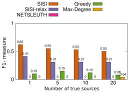
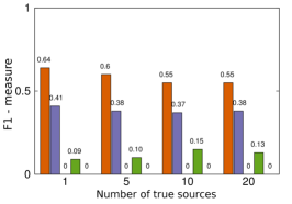
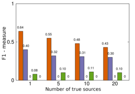
True source discovery. Fig. 5 reports the F1-measure scores of the tested algorithms. Note that this score has not been used in previous works [25, 23] since previous methods can only find nodes that are within few hops from the sources, but not the sources themselves. As shown in the figure, SISI and SISI-relax have the best performance. More than 50% of the true sources was discovered by SISI and 35% by SISI-relax that exquisitely surpass NETSLEUTH, Max-Degree with 0% and Greedy with roughly 10%.

#src	SISI	SISI-relax	NETS.	Greedy	Max-Degree
1	91.4	84.2	0	14.5	0
5	79.7	53.9	0	15.2	0
10	74.1	52.3	0	11.8	0
20	77.3	56.5	0	9.6	0

Table 3: True sources detected (%) with $|V_{I}|=1000$.

We also present the true source detected rates of different methods in Tab. 3 since this is an important aspect (positive rate) of ISI problem. The table shows accurate detection of SISI and SISI-relax. More than 70% and 50% of true sources are identified by SISI and SISI-relax respectively while NETSLEUTH and Max-Degree cannot detect any source.

Symmetric difference. Tab. 2 shows the $\mathbb{E}[D(S,\tau,V_{I})]$ values where $S$ is the returned solution of each algorithm with various number of true sources and sizes of infection cascades. In all the cases, SISI largely outperforms the other methods and obtains very close values to the true sources. The superiority of SISI against the SISI-relax and Greedy confirms the good solution guarantee of SISI. NETSLEUTH and Max-Degree optimize different criteria, i.e., description length (MDL) and node degree, and thus show poor performance in terms of symmetric difference. SISI-relax is consistently the second best method and preserves very well the performance of SISI.

Jaccard distance. We use $Q_{JD}(S)$ as in [25] to evaluate the algorithms and plot the results in Tab. 2. In this case, the closer value of $Q_{JD}(S)$ to 1 indicates better solution. In terms of $Q_{JD}(S)$, we observe the similar phenomena as measured by symmetric difference that SISI achieve drastically better solution than the others and the results of SISI-relax approach those of SISI very well with much fewer RR sets.

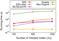
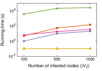
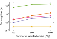
Comparing running time. Fig. 6 illustrates the running time of the algorithms in the previous experiments. We see that SISI is slower than NETSLEUTH and SISI-relax but the differences are minor while it provides by far better accuracy than other algorithms. SISI-relax obtains possibly the best balance among all: faster than NETSLEUTH and providing good solution quality as shown previously.

5.3 Experiments on the IC model

Set up. We compare SISI with the dynamic programming algorithm, temporarily called k-effector, in [20] when the infection process follows the IC model. Similar to other experiments, we simulate the infection process under the IC model with 4 different numbers of sources, i.e., 1, 5, 10, 20 and run SISI and k-effector on the resulting cascades. For each setting, we carry 10 simulations and report the average results. Note that the solution for k-effector in [20] requires the number of sources as an additional input parameter and for simplicity, we provide the true number of sources used in the simulation processes. SISI, however, do not require this information. We report the results in Table 4.

#src	Symmetric Difference			F1-measure
	SISI	k-effector	Max-Deg.	SISI	k-effector	Max-Deg.
1	6.6	18.4	42.3	0.57	0	0.02
5	55.1	103.4	176.9	0.53	0.02	0
10	25.2	72.6	154.1	0.49	0.03	0
20	203.7	295.2	384.7	0.52	0.05	0.03

Table 4: Comparison under the IC model.

Results. It is clear from Table 4 that SISI massively outperforms k-effector in terms of both symmetric difference and true source recovering ability. In summary, for any value of the number of true sources $k$, SISI always returns solution with symmetric difference equal half of the one returned by k-effector. In terms of true source discovery ability, while k-effector almost detects none of the true sources, SISI consistently achieves the F1-measure of at least 50%.

6 Discussion and Conclusion

We present SISI the first approximation algorithm for multiple source detection in general graphs which also works very well in practice. The algorithm can be extended to several other diffusion models and settings with little modification on the sampling procedure as outlined below.

Incomplete Observation [12, 15]. In many cases, we can only observe the states (infected/not infected) for a subset $O\subsetneq V$ of nodes in the network. In those cases, we need to modify the Fast TRIS sampling Algorithm in Line 1 and pick a node $u$ uniformly in $O$ (instead of $V$) and allow the sources to be from $V_{I}$ or unknown state nodes.

However, the SISI cannot be directly adapted to non-progessive models in which a node can switch from an infected state into uninfected state. Thus approximation algorithm for source detection in non-progressive models leaves an open question and is among our future work.

References

- [1] http://www.pcworld.com/article/163920/swine_flu_twitter.html.
- [2] http://fox13now.com/2013/04/24/the-power-of-one-wrong-tweet/.
- [3] http://www.businessinsider.com/reddit-falsely\-accuses-sunil-tripathi-of-boston-bombing-2013-7.