A two-scale approach for efficient on-the-fly operator assembly in massively parallel high performance multigrid codes

Abstract.

Matrix-free finite element implementations of massively parallel geometric multigrid save memory and are often significantly faster than implementations using classical sparse matrix techniques. They are especially well suited for hierarchical hybrid grids on polyhedral domains. In the case of constant coefficients all fine grid node stencils in the interior of a coarse macro element are equal. However, for non-polyhedral domains the situation changes. Then even for the Laplace operator, the non-linear element mapping leads to fine grid stencils that can vary from grid point to grid point. This observation motivates a new two-scale approach that exploits a piecewise polynomial approximation of the fine grid operator with respect to the coarse mesh size. The low-cost evaluation of these surrogate polynomials results in an efficient stencil assembly on-the-fly for non-polyhedral domains that can be significantly more efficient than matrix-free techniques that are based on an element-wise assembly. The performance analysis and additional hardware-aware code optimizations are based on the Execution-Cache-Memory model. Several aspects such as two-scale a priori error bounds and double discretization techniques are presented. Weak and strong scaling results illustrate the benefits of the new technique when used within large scale PDE solvers.

^a Dept. of Earth and Environmental Sciences, Ludwig-Maximilians-Universität München, 80333 München, Germany
^b Dept. of Computer Science 10, FAU Erlangen-Nürnberg, 91058 Erlangen, Germany
^c Erlangen Regional Computing Center (RRZE), FAU Erlangen-Nürnberg, 91058 Erlangen, Germany
^d Institute for Numerical Mathematics (M2), Technische Universität München, 85748 Garching b. München, Germany
^e Leibniz Supercomputing Center (LRZ), 85748 Garching b. München, Germany

Keywords. two-scale, massively parallel multigrid, matrix free, on-the-fly assembly, ECM-model, scaling results, surrogate operator

1. Introduction

In many real-life applications, e.g., from structural mechanics, fluid dynamics, or geophysics, a simulation method may have to accommodate curved boundaries of the computational domain, see e.g. [1, 2, 3, 4]. In particular, one of the grand challenges in geophysics are Earth mantle simulations where the domain is a thick spherical shell. Here, patch-wise defined isogeometric elements can achieve a high accuracy per degree of freedom. However, to date no high performance implementation exists on peta-scale supercomputer systems.

Classical low order finite elements are well-established also as highly efficient parallel implementations. Nevertheless, large scale applications often require a careful, memory aware realization. For instance, the global resolution of the Earth mantle with 1 km already leads to a mesh with $10^{12}$ nodes. Then the solution vector for a scalar PDE operator requires 8 TByte of memory. Such a large vector still fits well in the aggregate memory of current peta-scale supercomputers such as SuperMUC that we will use for our scalability experiments in Sec. 6.

This becomes different, when we consider storing the stiffness matrix. For linear tetrahedral elements on average 15 non-zeros are generated per matrix row. Then, even in classical compressed row sparse (CRS) matrix format [5], such a matrix of dimension $10^{12}$ will require 240 TByte of storage and this may drive even large computers beyond their limits. While developing more efficient sparse matrix techniques is an active field of research, see e.g. [6, 7, 8], pre-computing and storing the entries of the stiffness matrix inevitably requires a vast amount of memory and in turn produces massive memory traffic in the solution phase of the algebraic system, [9]. We point out that transferring large amounts of data from memory to the CPU is considered to be a critical cost factor, e.g. in terms of energy consumption. We also note that memory caching as well as spatial and temporal blocking techniques can be used to alleviate this problem [10, 11], but that their benefit is also limited.

To avoid the bottleneck of storing huge matrices, so-called matrix-free approaches [12, 13, 14, 15, 16] must be employed when possible. Here all matrix entries are re-computed on-the-fly when needed. We refer to [17, 18, 19, 20, 21, 22] for state of the art massively parallel solvers for PDEs and to [23, 24, 25] for large scale applications in geophysics.

For polyhedral domains, matrix-free methods can exploit the structure of uniformly refined mesh sequences. Here simple on-the-fly assembly routines can be developed that make use of the similarity of the finite elements in the refinement hierarchy. In this case, the performance depends essentially on exploiting the redundancy in the mesh structure. However, the situation is more complex for non-polyhedral domains. A naïve approach which ignores the physically correct domain and resolves the geometry only with respect to a coarser mesh will result in a reduced accuracy. The cheapest version, using a fixed non-exact resolution of the geometry will, in general, result asymptotically in a loss of convergence.

Resolving the geometry by nodal low order interpolation and using affine element mappings, gives optimal order results for linear finite elements. However, resolving the geometry more and more accurately with increasing refinement level is computationally expensive, since now the refinement process generates new non-similar elements and thus the local assembly process cannot profit to the full extent from the uniform refinement structure. These fundamental observations are the reason why current matrix-free codes reach significantly better performance on polyhedral domains than in more general geometries.

The main contribution of this article is a novel technique that improves the performance of matrix-free techniques in the case of complex geometries and curved boundaries without sacrificing accuracy. To achieve this, we will propose and analyze a new two-scale combination of classical interpolation with finite element approximations.

The outline of the paper is as follows: We start with the formulation of the model problem and a brief discussion of hybrid hierarchical grids in Sec. 2. In Sec. 3, we introduce the new two-scale method based on a higher order polynomial approximation of the low order finite element stencil presentation. We discuss two different variants using standard interpolation and least square fitting techniques and comment on a priori estimates. In Sec. 4, we focus on a study of the numerical accuracy and cost considerations. The influence of the polynomial degree in the stencil approximation on the accuracy as well as the effect of a double discretization [26] used for residual computation and smoother application is illustrated. Sec. 5 is devoted to the kernel optimization as it is essential for large scale high performance computations. The analysis is based on an enhanced Execution-Cache-Memory (ECM) model. Finally in Sec. 6, we present weak and strong scaling results on a current peta-scale architecture.

2. Model problem and hybrid hierarchical meshes

Matrix-free implementations of finite element schemes for partial differential equations are attractive on modern heterogeneous architectures. However, special care is required in the case of PDEs on domains with curvilinear boundary surfaces or interfaces. Here we propose a novel two-scale scheme that is perfectly suited to large scale matrix-free geometric multigrid solvers for low order conforming finite element discretizations.

2.1. Model problem

We consider the Laplace equation with homogeneous Dirichlet boundary conditions on a spherical shell as our model problem

(1) $$-\Delta u=f\quad\text{in }\Omega\quad\text{and}\quad u=0\quad\text{on }\partial\Omega$$

where $\Omega:=\{(x,y,z)\in\mathbb{R}^{3}:r_{1}^{2}<x^{2}+y^{2}+z^{2}<r_{2}^{2}\}$ with $0<r_{1}<r_{2}$ and $f\in L^{2}(\Omega)$. But we point out, that our approach can be also applied for more complex systems of PDEs, variable coefficients PDEs and general geometries.

The standard Galerkin formulation of (1) reads as: find $u\in H_{0}^{1}(\Omega)$ which satisfies

(2) $$a(u,v)=(f,v)\qquad\forall v\in H_{0}^{1}(\Omega)$$

where the bilinear and linear forms are given by

$$a(u,v):=\langle\nabla u,\nabla v\rangle_{\Omega}\enspace,\quad(f,v):=\langle f,v\rangle_{\Omega},$$

for all $u,v\in H^{1}_{0}(\Omega)$.

2.2. Domain and finite element approximations

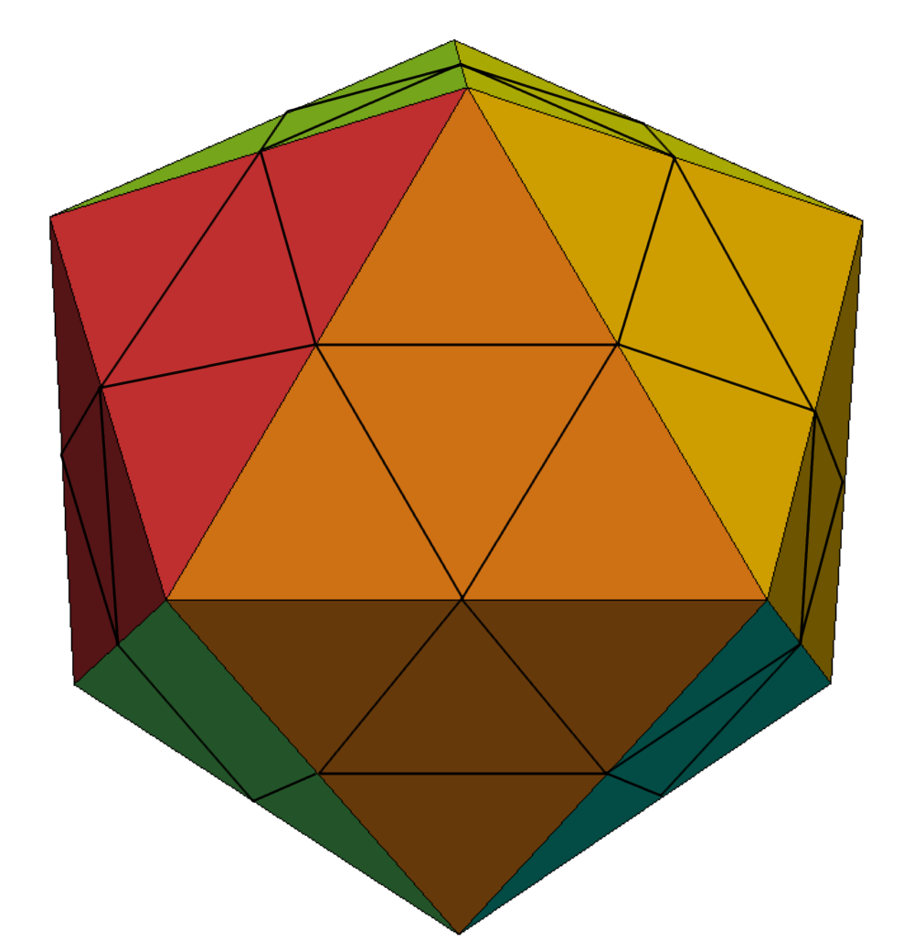
If a polyhedral domain is considered, the input mesh can be selected such that the domain is equal to the union of all elements of the mesh. Thus, the domain can be represented exactly. However, for our model domain of a spherical shell this is not possible when using tetrahedra that are affinely mapped from the reference tetrahedron $\hat{T}$ with nodes $(0,0,0)$, $(1,0,0)$, $(0,1,0)$ and $(0,0,1)$. We use two different sequences of triangulations. Both of them are based on a possibly unstructured simplicial initial mesh $\mathcal{T}_{-2}$ of meshsize $H$ defining $\overline{\Omega}_{H}:=\cup_{T\in\mathcal{T}_{-2}}\overline{T}$. We start by constructing a hierarchy of uniformly refined triangulations $\mathcal{T}:=\{\mathcal{T}_{\ell},\,\ell=0,1,\dots,L\}$ based on successive regular refinement [27].

Figure 2.1. Approximation of spherical shell with $\mathcal{T}_{-1}$ (left) and $\tilde{\mathcal{T}}_{-1}$ (right).

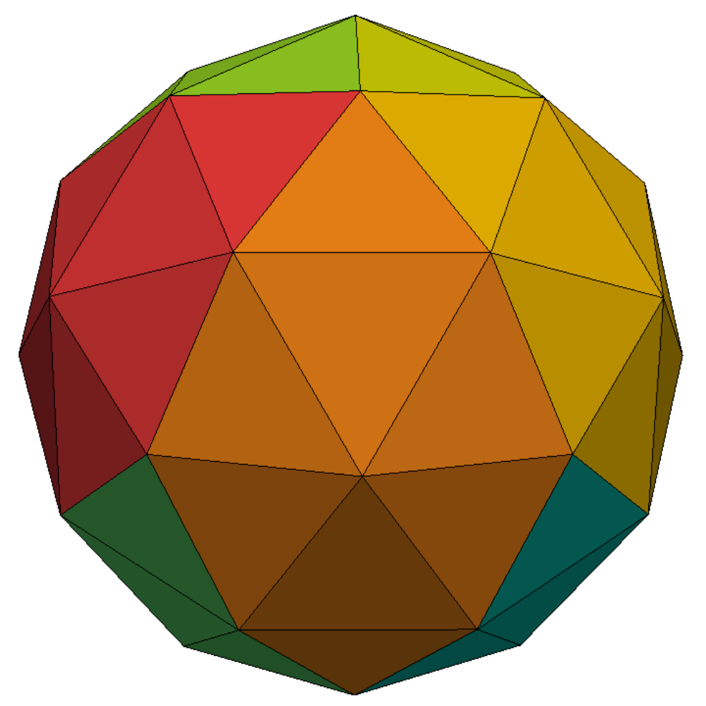We refer to the elements of $\mathcal{T}_{-2}$ as macro elements and point out that our notation guarantees that each macro element has at least one inner node for every mesh in the sequence $\mathcal{T}$. The level mesh-size is given by $h_{\ell}=2^{-(\ell+2)}H$. For each mesh $\mathcal{T}_{\ell}\in\mathcal{T}$, we find $\overline{\Omega}_{H}=\cup_{T\in\mathcal{T}_{\ell}}\overline{T}$. Consequently, the quality of the geometry approximation is fixed and does not improve with increasing refinement level. Therefore in a subsequent step, we project all refined nodes onto the spherical surface.

Figure 2.2. Sketch of the different macro element mappings. In the reference domain (left) nodes are associated with the discrete indices $(i,j,k)$. Here $k$ is fixed to get a 2D clipping and we call it an index plane. Firstly the reference domain is affinely mapped by $\Psi_{T}$ to the physical coordinates. This is the standard HHG domain (center). Secondly, the macro element $T$ is mapped by $\Phi_{T}$ to the projected element (right).

This is schematically illustrated for one macro element by a 2D clipping in Fig. 2.2. Firstly, the reference element $\hat{T}$ is affinely mapped by $\Psi_{T}$ onto a macro element $T$ in $\mathcal{T}_{-2}$. Secondly, $T$ is mapped by a blending function $\Phi_{T}$ reflecting the domain of interest. In case of a polyhedral domain, $\Phi_{T}$ can be selected as identity and in more general but piecewise smooth settings, we have $\|(\Phi_{T}-{\rm Id})\circ\Psi_{T}\|_{\infty}={\mathcal{O}}(H^{2})$. We refer to [28] for an explicit proof in 2D if $\Phi_{T}$ is defined by a smooth surface representation. Note that in our case the mapping $\Phi_{T}$ is also done for the interior elements of $\mathcal{\widetilde{T}}_{-2}$, such that they form spherical layers.

Now, we define the global mapping $\Phi$ elementwise by $\Phi|_{T}:=\Phi_{T}$ and assume that $\Phi$ is globally continuous and $\Phi(\Omega_{H})=\Omega$. In terms of $\Phi$, we obtain a second family $\mathcal{\widetilde{T}}:=\{\mathcal{\widetilde{T}}_{\ell}\}_{{}_{\ell}}$ of simplicial triangulations as follows: The vertices of $\mathcal{\widetilde{T}}_{\ell}$ are obtained by an application of $\Phi$ on the vertices of $\mathcal{T}_{\ell}$, and the edge graphs are topologically equivalent to the ones of $\mathcal{T}$, i.e., the node connectivity remains unchanged. Under the assumption that $\Phi$ is a piecewise smooth bijection, $\mathcal{\widetilde{T}}$ satisfies a uniform shape regularity and standard a priori finite element estimates holds. Moreover the vertices of $\mathcal{\widetilde{T}}_{\ell}$ are also vertices of $\mathcal{\widetilde{T}}_{\ell+1}$. However the midpoints of the edges on level $\ell$ are, in general, not the new vertices on level $\ell+1$. Consequently the arising sub-elements are not similar to one of the three sub-element classes which occur, if one tetrahedron is uniformly refined, see also Fig. 2.3.

Typically, low order finite element approximations are then based on the mesh sequence $\mathcal{\widetilde{T}}$ and not on $\mathcal{T}$. The standard finite element space is defined as

$$V_{\ell}=\{v\in H_{0}^{1}(\Omega_{\ell}):v|_{T}\in P_{1}(T),~{}\forall\,T\in\mathcal{\widetilde{T}}_{\ell}\},$$

where $\overline{\Omega}_{\ell}:=\cup_{T\in\mathcal{\widetilde{T}}_{\ell}}\overline{T}$. We point out that $\Omega_{\ell}$ forms a sequence of domains approximating $\Omega$ and that due to the domain approximation $V_{\ell}\not\subset V_{\ell+1}$. The discrete Galerkin formulation of (2) then reads as: find $u_{\ell}\in V_{\ell}$ that satisfies

(3) $$a_{\ell}(u_{\ell},v_{\ell})=\langle f,v_{\ell}\rangle_{\Omega_{\ell}}\qquad\forall v_{\ell}\in{V}_{\ell}$$

where $a_{\ell}(\cdot,\cdot):=\langle\nabla\cdot,\nabla\cdot\rangle_{\Omega_{\ell}}$. Let $\{\phi_{I}\}_{I}$ be the nodal basis of $V_{\ell}$; for simplicity we ignore in the notation of $\phi_{I}$ the level index $\ell$, if there is no ambiguity. Then this transforms to the algebraic system

(4) $$\mathcal{L}_{\ell}\mathbf{u}_{\ell}=\mathbf{f}_{\ell}$$

where $\mathbf{u}_{\ell}$ denotes the vector of nodal values of the finite element approximations, i.e., $u_{\ell}=\sum_{I}(\mathbf{u}_{\ell})_{I}\phi_{I}$, and $\mathbf{f}_{\ell}$ stands for the algebraic representation of the linear form $(\mathbf{f}_{\ell})_{I}=\langle f,\phi_{I}\rangle_{\Omega_{\ell}}$. As it is standard, the entries of $\left(\mathcal{L}_{\ell}\right)_{I,J}$ are given by $a_{\ell}(\phi_{I},\phi_{J})$. The standard matrix formulation (4) can be related to a representation of $\mathcal{L}_{\ell}$ in stencil form, i.e., each line of the matrix is associated with a node $I$, and its non-zero entries form the weights of the associated node stencil $s^{I}$.

2.3. Hybrid hierarchical mesh stencils

Massively parallel and highly scalable PDE software frameworks depend on a sophisticated data structure based on ghost layers. To reduce communication and memory traffic, the abstract concept of different hierarchical primitives can be applied. Here we use the hybrid hierarchical grids (HHG) framework which provides an excellent compromise between flexibility and performance [13, 29, 30]. While the coarse mesh can be completely unstructured, the fine mesh is obtained by uniform refinement following the rules given in [27]. Each element is refined into eight sub-elements each of which belongs to one of three different sub-classes, see the left of Fig. 2.3. All nodes $I$ of the triangulation can then be grouped into vertex, edge, face or volume primitives depending on their position within one macro element. The vertex, edge and face primitives form the lower primitive classes. Such a structured block refinement then guarantees in the case of affine element mappings that the node stencils for partial differential equations with constant coefficients do not depend on the node location within one primitive. More precisely for each macro element, all volume primitive stencils are exactly the same and are given by a symmetric 15-point stencil, see the right of Fig. 2.3.

Figure 2.3. 15-point stencil (right) and the three classes of sub-tetrahedra (left).

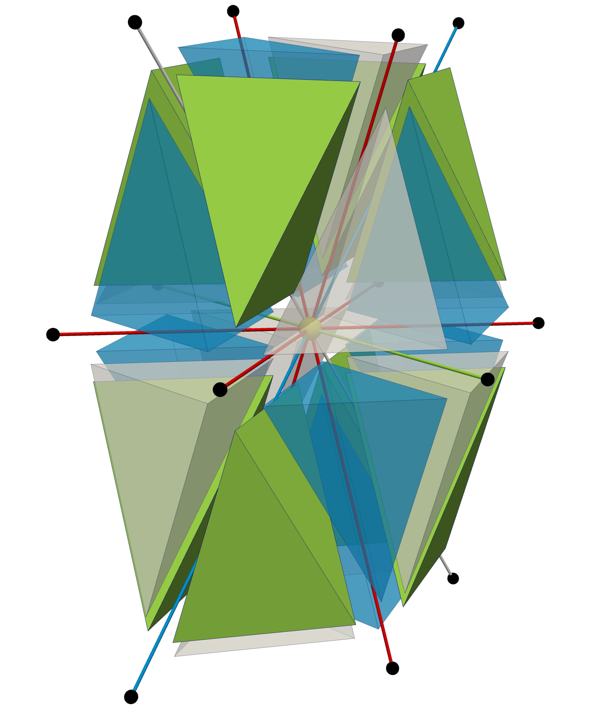
In large scale applications, the number of nodes in the volume primitive containers is significantly higher than the number of nodes in the lower primitive classes. It grows with ${\mathcal{O}}(2^{3\ell})$ whereas the number of remaining nodes increases only with ${\mathcal{O}}(2^{2\ell})$. Since we are interested in large scale simulations, the computational cost associated with the node stencils on the lower primitives is rather small compared to the cost associated with the nodes in the volume primitives. Thus we compute on-the-fly the nodes stencils for nodes in a lower primitive class in a straightforward way by reassembling the contributions of local stiffness matrices. Only the on-the-fly computation of the node stencils for nodes in a volume primitive class will be replaced by a surrogate stencil operator. We recall that the volume primitives are associated with the macro elements. Let $T\in\mathcal{T}_{-2}$ be fixed, then we denote by $\mathcal{M}_{\ell}$ the set of all interior points of $T$. These nodes are within the volume primitive associated with $T$, at refinement level $0\leqslant\ell\leqslant L$. For $\ell=0$ this consists of exactly one single point. The number $n_{\ell}$ of elements in $\mathcal{M}_{\ell}$ is given by

(5) $$n_{\ell}=\frac{\left(2^{\ell+2}-3\right)\left(2^{\ell+2}-2\right)\left(2^{\ell+2}-1\right)}{6}.$$

Remark 1.

We point out that all our techniques can also be applied to the construction of stencil entries associated with face and edge nodes. This is of interest in case of moderate level hierarchies.

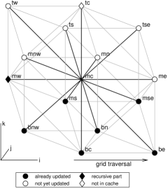
For a fixed node $I$, the stencil weight for accessing another node $J$ is given by $a_{\ell}(\phi_{I},\phi_{J})$ and will only be non-zero, if both nodes are connected by an edge in $\mathcal{T}_{\ell}$. In case of our uniform mesh refinement, the stencil weights can be identified by their cardinal directions $w\in\mathcal{W}=\{be,bc,...,mc\}$, where, as noted before, we have $|\mathcal{W}|=15$. The first character in $w$ denotes the bottom, middle and top plane whereas the second specifies the orientation within the plane, as illustrated in Fig. 2.4. Then the stencil for node $I$ can be represented by a vector $s^{I}=(a_{\ell}(\phi_{I},\phi_{J_{be}}),$ …,$a_{\ell}(\phi_{I},\phi_{J_{mc}}))$ in $\mathbb{R}^{15}$. We note that $J_{mc}=I$.

Figure 2.4. Layout of a typical low order 15pt stencil; see also [29]; node symbols will be relevant in Sec. 5.

Moreover there exists a unique mapping between the nodes in ${\mathcal{M}}_{\ell}$ and the set of index triples ${\mathcal{I}}_{\ell}$ given by

$$\{(i,j,k);0<i,j,k<2^{\ell+2}-2,i+j+k<2^{\ell+2}\}.$$

Hence the node stencils on level $\ell$ can be associated with a stencil function $s:{\mathcal{I}}_{\ell}\rightarrow\mathbb{R}^{15}$, i.e. $s^{I}=s(i_{I},j_{I},k_{I})$ where $(i_{I},j_{I},k_{I})$ is the index triple associated with node $I$. If $\Phi=\text{Id}$ then all $s^{I}$, $I\in{\mathcal{M}}_{\ell}$ are the same, i.e., $s$ is a constant function. Moreover it is obtained by simple scaling from a reference stencil $\hat{s}$, i.e., $s^{I}=2^{-\ell}\hat{s}$, $I\in{\mathcal{M}}_{\ell}$, with $\hat{s}$ being the stencil associated with the single node in ${\mathcal{M}}_{0}$. This is not the case for our model domain. Here $s$ is a non-constant function and consequently all stencil weights have to be computed on-the-fly. To do so for each node $I\in{\mathcal{M}}_{\ell}$, we have to consider the 24 tetrahedra adjacent to it and their associated local stiffness matrices which can be different from element to element due to a general $\Phi$. Thus this process, although linear with respect to $n_{\ell}$, can be rather cost intense. For $L=6$ we have to compute on-the-fly $2,731,135$ different stencils per macro element.

Figure 2.5. Uniformly refined reference tetrahedron. Highlighted plane shows the location of nodal centers for the stencils visualized in Fig. 2.6 and Fig. 3.1. Black dots mark the ten sampling points for IPOLY (Sec. 3.1).

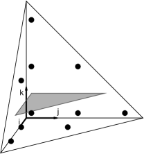
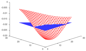
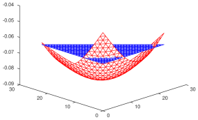
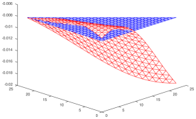
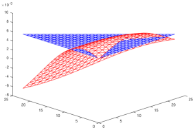
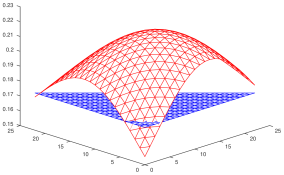
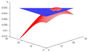
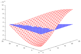
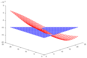
In Fig. 2.6, we illustrate the influence of $\Phi$ on the node stencil restricted to an index plane, see Fig. 2.5. Note that for $\Phi=\text{Id}$ not only the stiffness matrix but also the stencil is symmetric, i.e., opposite stencil entries, e.g., tw and be, are identical. While this kind of symmetry is not completely preserved in the more general case, it is still reflected. Hence, we show only seven stencil entries plus the central one in Fig. 2.6. One can clearly see that the stencil entries are smooth functions that can be easily approximated by polynomials. This observation motivates our new approach.

(a) $w=tc$	(b) $w=ts$
(c) $w=mw$	(d) $w=mn$
(e) $w=mc$	(f) $w=mse$
(g) $w=bnw$	(h) $w=be$

Figure 2.6. Eight out of the 15 stencil values associated with the uniformly refined mesh series $\mathcal{T}$ (blue) and the projected series $\mathcal{\widetilde{T}}$ (red). Each subplot shows the stencil values of one $w\in\mathcal{W}$ for all fine grid nodes in the plane $k=7$ of a macro element at refinement level $\ell=3$. Here the x,y location corresponds to the i,j index of the nodes, and the z-direction shows the stencil value. The fixed $k$ index is chosen such that it contains the median node.

3. Two-scale approach

Our idea now is to replace the components of the exact stencil function $s$ associated with a volume primitive node by surrogate polynomials of moderate order. More precisely, we consider for each cardinal direction $w\in{\mathcal{W}}$ a polynomial defined either by interpolation or alternatively by a discrete $L^{2}$-best fit. We will only perform the replacement of the stencil function on levels $\ell\geqslant 1$ as on the coarsest level $\ell=0$ a macro element has only one interior node with a single associated stencil.

3.1. Interpolation of stencils (IPOLY)

A tri-variate polynomial of degree less or equal to $q$ can be represented as

(6) $$p(i,j,k)=\sum_{\begin{subarray}{c}l,m,n=0\\ l+m+n\leqslant q\end{subarray}}a_{l,m,n}\lambda_{l,m,n}(i,j,k)\enspace,$$

where the $\lambda_{l,m,n}$ form a basis. Solving for the coefficients $\mathbf{a}=(a_{q00},...,$ $a_{000})\in\mathbb{R}^{m_{q}}$ where

(7) $$m_{q}=\frac{1}{6}(q+3)(q+2)(q+1)$$

of an interpolation polynomial in general leads to a linear system $A\mathbf{a}=\mathbf{b}$ with a Vandermonde-type matrix $A\in\mathbb{R}^{m_{q}\times m_{q}}$ and sampling values $\mathbf{b}\in\mathbb{R}^{m_{q}}$. The special choice of a Lagrange interpolation basis yields $A=\text{Id}$. As example, we consider the case $q=2$. Here we have $m_{2}=10$ and for sampling we use the quadratic nodal interpolation points of a shrunk macro element. More precisely we use the nodes with indices

$$(1,1,1),\enspace(1,1,a),\enspace(1,a,1),\enspace(a,1,1),$$

$$(1,1,b),\enspace(1,b,1),\enspace(b,1,1),$$

$$(1,b,b),\enspace(b,1,b),\enspace(b,b,1)$$

where $a=2^{\ell+2}-3$, $b=2^{\ell+1}-1$ as sampling points, see also Fig. 2.5.

3.2. Least-squares approximation (LSQP)

Applying an interpolation polynomial implies that the polynomial is exact at the sampling points, which elevates these points. Alternatively, we can use a discrete $L^{2}$-best approximation polynomial. This leads to a system with an $n_{\ell}\times m_{q}$ matrix, as we now use all points of $\mathcal{M}_{\ell}$ as our sampling set $\mathcal{S}_{\ell}$. More generally, we define the coefficients $\mathbf{a}$ of the approximating polynomial as solution of the least-squares problem

$$\mathbf{a}:=\operatorname*{argmin}_{\mathbf{z}\in\mathbb{R}^{m_{q}}}\|A\mathbf{z}-\mathbf{b}\|_{2}\enspace,$$

$$A\in\mathbb{R}^{|\mathcal{S}_{\ell}|\times m_{q}}\>,\,\mathbf{b}\in\mathbb{R}^{|\mathcal{S}_{\ell}|}\enspace.$$

Each row of $A$ is defined by the values of the basis functions $\lambda_{l,m.n}$ evaluated at the corresponding sampling point. The choice $\mathcal{S}_{\ell}=\mathcal{M}_{\ell}$ quickly becomes quite expensive, due to the fast growth of $n_{\ell}$ with $\ell$. Thus we also consider reduced sampling sets $S_{\ell}:=\mathcal{M}_{m(\ell,j)}$ with

(8) $$m(\ell,j):=\min\{\ell,\max\{1,j\}\}$$

where $j$ may depend on $\ell$. The min-max definition guarantees that we neither exceed the largest possible set, i.e., $\mathcal{M}_{\ell}$ on level $\ell$, nor go below $\mathcal{M}_{1}$. For simplicity of notation, we also denote $\mathcal{M}_{m(\ell,j)}$ by $\mathcal{M}_{j}$ if there is no ambiguity.

We note that for $q\leqslant 4$, the matrix $A$ has full rank for any choice of $S_{\ell}=\mathcal{M}_{k}$ with $k\in\{1,\ldots,\ell\}$. This is easily seen by comparing (5) and (7) and considering the spatial distribution of the nodes in the mesh. Consequently the least-squares problem will then have a unique solution.

3.3. IPOLY versus LSQP for quadratic surrogate polynomials

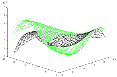
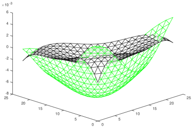
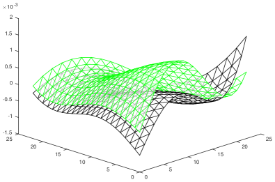
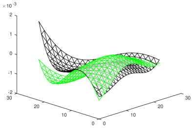
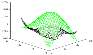
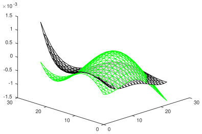
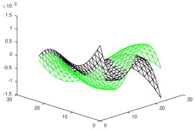
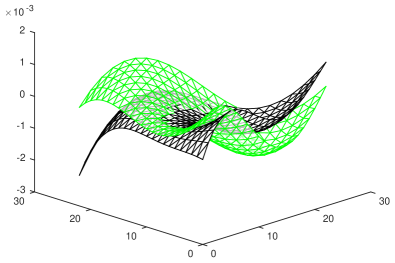
In a first test, we compare the difference between the least-squares technique for ${\mathcal{S}}_{\ell}={\mathcal{M}}_{\ell-1}$ and the interpolation based approach, see Fig. 3.1. Note that, as in Fig. 2.6, the points visualized are chosen to be in the plane with $k=7$. Hence the displayed corners are no sampling points for IPOLY. While the values of IPOLY are more accurate close to the boundary, the values of LSQP have an uniformly better fit.

(a) $w=tc$	(b) $w=ts$
(c) $w=mw$	(d) $w=mn$
(e) $w=mc$	(f) $w=mse$
(g) $w=bnw$	(h) $w=be$

Figure 3.1. Difference between IFEM and IPOLY (green) or LSQP (black) for the same setting than in Fig. 2.6.

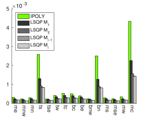
In order to provide a more quantitative measure for the approximation accuracy, we introduce two metrics, one for the overall fit and one for the maximal deviation. For $w\in{\mathcal{W}}$ we set

$$e_{w}^{2} :=\sqrt{\sum_{(i,j,k)\in{\mathcal{I}}_{\ell}}\frac{\left[s_{w}(i,j,k)-\mathcal{P}^{\alpha}{s}_{w}(i,j,k)\right]^{2}}{n_{\ell}}}$$

$$e_{w}^{\infty} :=\max_{(i,j,k)\in{\mathcal{I}}_{\ell}}\left|{s}_{w}(i,j,k)-\mathcal{P}^{\alpha}{s}_{w}(i,j,k)\right|\,,$$

where $\mathcal{P}^{\alpha}s_{w}$, $\alpha\in\{\textsc{LSQP},\textsc{IPOLY}\}$, denotes one of the proposed surrogate polynomials associated with the cardinal direction $w\in{\mathcal{W}}$. Obviously these two metrics correspond to the discrete $L^{2}$ and $L^{\infty}$ norms of the error in approximating the $w$-th component of the stencil function $s$.

Figure 3.2. $e_{w}^{2}$ (left) and $e_{w}^{\infty}$ (right) for IPOLY and LSQP with different choices for the sampling set. Macro mesh consists of 60 elements and $L=4$.

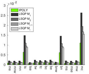In Fig. 3.2, we illustrate the influence of the choice of the sampling set on LSQP and compare it to the IPOLY approach. We observe two peaks for the off-center values and consequently also one in the center stencil entry. The mapping function $\Phi$ depends on the location of the macro element within the spherical shell and determines which $w\in{\mathcal{W}}$ is more strongly affected by the approximation. Comparing LSQP and IPOLY we find that the maximal difference for LSQP is higher while the $L^{2}$ fit is better by construction. Already for the smallest sampling set ${\mathcal{M}}_{1}$, i.e., $n_{1}=35$, it is significantly better than for IPOLY. We note that ${\mathcal{M}}_{2}$, i.e., $n_{2}=455$, is, in general, a good compromise, in particular if the number of macro elements is already large.

3.4. Definition of the surrogate operator

We define our new two-scale finite element approximation as the solution of

(9) $$\mathcal{L}_{\ell}^{H,\alpha,q}\mathbf{u}_{\ell}^{H,\alpha,q}=\mathbf{f}_{\ell}.$$

Here, the superscripts mark the dependencies on the macro element size $H$, the degree $q$ of the surrogate polynomial, and the selected approach $\alpha\in\{\textsc{IPOLY},\textsc{LSQP}\}$. For ease of notation, we replace the superscript triple by a tilde, i.e., we set $\widetilde{\mathcal{L}}_{\ell}:=\mathcal{L}_{\ell}^{H,\alpha,q}$ and similarly for $\mathbf{u}_{\ell}^{H,\alpha,q}$.

As is the case with $\mathcal{L}_{\ell}$, each row of $\widetilde{\mathcal{L}}_{\ell}$ is associated with a node. In our approach, we replace for all nodes in a volume primitive the exact finite element stencil on level $\ell$ by its surrogate polynomial approximation, i.e., instead of computing $s_{w}(i,j,k)$ on-the-fly, we evaluate the surrogate ${\mathcal{P}}^{\alpha}s_{w}(i,j,k)$. As already mentioned, the stencil entries associated with nodes on lower dimensional primitives are assembled on-the-fly in standard fashion.

Remark 2.

We point out that, if $\Phi_{T}=\text{Id}$, $T\in{\mathcal{T}}_{-2}$, then both our approaches reduces to the standard one. Also, they can be applied selectively, and switched on or off macro element-wise depending on the location of $T$ within the domain or its shape. Additionally the choice of the polynomial degree can depend on $T$, and we can even use anisotropic orders reflecting the properties of the mapping $\Phi_{T}$.

Since we have one stencil weight for each of the 15 couplings $w\in\mathcal{W}$, we use 15 different second order polynomials, described by 15 different sets of coefficients $\mathbf{a}_{w}$. The latter are computed in a setup phase. This, firstly, requires for each macro element and each level $\ell\geqslant 1$ the evaluation of $m_{q}$ (IPOLY) or $|\mathcal{S}_{\ell}|$ (LSQP) stencils and then the solution of a linear or least-squares system.

Once the setup is completed, whenever the stencil for node $I$ is to be applied, e.g. as part of a smoothing step in a multigrid method, or a residual computation, 15 polynomials of type (6) must be evaluated at this node to provide the surrogate stencil weights. At first glance, this does not seem to be any faster than a standard implementation. Recall, however, that within a typical matrix-free framework, the on-the-fly evaluation of the stencil involves costly operations such as the (re-)computation of local element matrices or the direct evaluation of weak forms via quadrature rules. The advantage of our approach is that the setup needs to be performed only once. The operator assembly itself reduces to polynomial evaluations. This also implies that the cost for the actual stencil application is the same for both, IPOLY and LSQP. Only in the setup phase is LSQP more expensive as more sampling points need to be evaluated and the minimization problem includes a larger system matrix.

Compared to a full stencil pre-calculation and storage scheme also the amount of required memory can be neglected. We only need $15m_{q}L$ coefficients per macro element to fully describe the approximated stencils. Such a small number of coefficients can easily be stored even when $L$ is large.

Remark 3.

Alternatively, one can think of using the same fine level surrogate polynomial to evaluate the stencils on the coarser meshes. A rigorous study of this effect on the multigrid convergence rate is beyond the scope of the paper.

We want to point out that in the application of the surrogate operator we loop over the indices $(i,j,k)$ in a line-wise fashion. This implies that we can always fix two of the three indices and, consequently, only need to evaluate a 1D and not a 3D polynomial. This reduces the cost significantly as the 1D polynomial has fewer terms. Evaluation of the 1D polynomial itself can be accomplished very efficiently by using a hierarchical recursion formula. More precisely starting from a single direct evaluation of $\hat{p}(i):={\mathcal{P}}^{\alpha}s_{w}(i,j_{0},k_{0})$, we can evaluate the polynomial incrementally in terms of $q$ basic operations. In computer graphics this technique is known as forward differencing [31, 32].

Apart from its cost, the accuracy of a numerical scheme is, of course, of major importance. In this context we provide the following lemma related to the consistency of the discretization expressed by $\widetilde{\mathcal{L}}_{\ell}$.

Lemma 1.

The row sum property of the stencil

$$\sum_{w\in\mathcal{W}}s_{w}^{I}=0$$

is preserved by IPOLY and LSQP.

Proof.

We recall that the coefficients of both our approaches can formally be obtained by solving a system of normal equations. As $A$ has full rank its solution is unique and

$$\mathbf{a}_{mc} =\left(A^{\top}A\right)^{-1}A^{\top}\mathbf{b}_{mc}$$

$$=-\left(A^{\top}A\right)^{-1}A^{\top}\sum_{\begin{subarray}{c}w\in\mathcal{W}\\ w\neq mc\end{subarray}}\mathbf{b}_{w}=-\sum_{\begin{subarray}{c}w\in\mathcal{W}\\ w\neq mc\end{subarray}}\mathbf{a}_{w}\,.$$

Thus, the row sum condition holds for the coefficients of the surrogate polynomials and, consequently, also for the stencil entries approximated by an evaluation of the polynomials at each node position. ∎

Finally, we recall that the matrix $\mathcal{L}_{\ell}$ is symmetric, as $a_{\ell}({\phi}_{I},{\phi}_{J})$ = $a_{\ell}({\phi}_{J},{\phi}_{I})$. This property is not preserved by our approach, due to the fact that the polynomials are evaluated at the nodes. Let $I$ be a node, and $J$ be the neighboring node which is reached, if we move from $I$ in cardinal direction $w$. By $w^{\text{o}}$, we denote the opposite cardinal direction, i.e., if we move from $J$ into the direction of $w^{\text{o}}$ then we recover $I$. In our approach, we find

$$(\widetilde{\mathcal{L}}_{\ell})_{IJ} ={\mathcal{P}}^{\alpha}s_{w}(i_{I},j_{I},k_{I})$$

$$(\widetilde{\mathcal{L}}_{\ell})_{JI} ={\mathcal{P}}^{\alpha}s_{w^{\text{o}}}(i_{J},j_{J},k_{J})\,.$$

To quantify this loss of symmetry, we measure it in the relative Frobenius norm. We consider

$$\frac{\|(\widetilde{\mathcal{L}}_{\ell}|_{T})^{\top}-\widetilde{\mathcal{L}}_{\ell}|_{T}\|_{{}_{F}}}{\|\mathcal{L}_{\ell}|_{T}\|_{{}_{F}}}\,.$$

Here $\widetilde{\mathcal{L}}_{\ell}|_{T}$ is the restriction of the global stiffness matrix to one macro element. As expected, for both IPOLY and LSQP we find that the relative non-symmetry is in $\mathcal{O}(h_{\ell})$.

Remark 4.

A symmetric matrix can also be recovered. One possibility is to only define seven cardinal directions, associated with the seven edge directions of a macro element. For this we identify the cardinal directions $w$ and $w^{\text{o}}$ and evaluate the surrogate polynomial at the center of the edge connecting two nodes. Note that in that case, we need to define the central stencil weight via the row sum condition. As we will see in Sec. 5, a direct evaluation of the row sum is more expensive than the evaluation of a surrogate polynomial of moderate order. Therefore we will not further consider this option. We also point out that the loss of symmetry can be considered as a small perturbation and does not prohibit using a conjugate gradient method as solver.

3.5. A priori estimate

In this section, we will present an a priori estimate for the IPOLY and LSQP discretization errors in the $L^{2}$-norm. Let $\mathbf{u}_{\ell}$ and $\mathbf{\tilde{u}}_{\ell}$ be the solution of (4) and (9), respectively, and $u$ the exact solution of (1).

Since $\widetilde{\mathcal{L}}_{\ell}$ can be interpreted as polynomial approximation of a smooth function, we assume that it can be written as

$$\widetilde{\mathcal{L}}_{\ell}=\mathcal{L}_{\ell}\left(\text{Id}+H^{q+1}\widetilde{B}_{\ell}\right)$$

with a suitable $\widetilde{B}_{\ell}$ satisfying

(10) $$\|\widetilde{B}_{\ell}\|\leqslant C_{q,\alpha}<\infty.$$

Here $\|\cdot\|$ denotes the Euclidean norm. We point out that our assumption is motivated by the assumed smoothness of $\Phi$ in combination with best approximation and interpolation results. Moreover by construction we preserve the row sum property, and thus the kernel of $\mathcal{L}_{\ell}$ and $\widetilde{\mathcal{L}}_{\ell}$ is locally the same. The notation $\lesssim$ is used for $\leqslant C$ with an $\ell,H$-independent constant $C<\infty$.

Furthermore, we assume that $H$ is chosen small enough such that $H^{q+1}\|\widetilde{B}_{\ell}\|<1$. By employing the properties of the Neumann series, we then obtain

$$\begin{split}\widetilde{\mathcal{L}}_{\ell}^{-1}&=\left(\text{Id}+H^{q+1}\widetilde{B}_{\ell}\right)^{-1}\mathcal{L}_{\ell}^{-1}\\ &=\left[\sum_{k=0}^{\infty}\left(-H^{q+1}\widetilde{B}_{\ell}\right)^{k}\right]\mathcal{L}_{\ell}^{-1}\\ &=\left(\text{Id}-H^{q+1}\widetilde{B}_{\ell}\right)\mathcal{L}_{\ell}^{-1}+\mathcal{O}\left(H^{2(q+1)}\right).\end{split}$$

Neglecting the higher order terms, we arrive at

$$\begin{split}\|\tilde{{u}}_{\ell}-{u}_{\ell}\|_{0}^{2}&\lesssim h^{3}\|\tilde{\mathbf{u}}_{\ell}-\mathbf{u}_{\ell}\|^{2}\\ &=h^{3}\|\mathcal{L}_{\ell}^{-1}\mathbf{f}_{\ell}-\widetilde{\mathcal{L}}_{\ell}^{-1}\mathbf{f}_{\ell}\|^{2}\\ &\lesssim h^{3}\|H^{q+1}\widetilde{B}_{\ell}\mathcal{L}_{\ell}^{-1}\mathbf{f}_{\ell}\|^{2}\\ &\lesssim h^{3}H^{2(q+1)}\|\widetilde{B}_{\ell}\|^{2}\|\mathbf{u}_{\ell}\|^{2}\\ &\lesssim H^{2(q+1)}\|\widetilde{B}_{\ell}\|^{2}\|u_{\ell}\|_{0}^{2}\>.\end{split}$$

It is well known that under suitable regularity assumptions $\|u-u_{\ell}\|_{0}\lesssim h_{\ell}^{2}\|f\|_{0}$. Then the triangle inequality yields

(11) $$\begin{split}\|u-\tilde{u}_{\ell}\|_{0}&\leqslant\|u-u_{\ell}\|_{0}+\|u_{\ell}-\tilde{u}_{\ell}\|_{0}\\ &\lesssim\left(h_{\ell}^{2}+H^{q+1}\right)\|f\|_{0}\\ &\lesssim h_{\ell}^{2}\left(1+4^{l+2}H^{q-1}\right)\|f\|_{0}\>.\end{split}$$

We note that the generic constants do possibly depend on $\alpha$ and $q$. Keeping $H$ fixed and increasing $\ell$ will result in an asymptotically constant error not equal to zero. However for $\ell\leqslant L$ and $L$ fixed and a small enough macro meshsize $H$, we obtain optimal order results in $h_{\ell}$, $q\geqslant 2$.

4. Evaluation of accuracy and cost

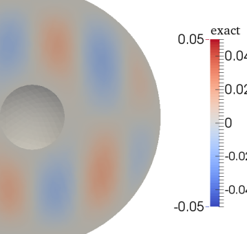
For our numerical studies, we employ model problem (1) with an exact solution given by

$$\bar{u}=(r-r_{1})(r-r_{2})\sin(10x)\sin(4y)\sin(7z)$$

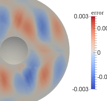
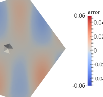
where $r=r(x,y,z)=\left(x^{2}+y^{2}+z^{2}\right)^{1/2}$. The right-hand side is set accordingly, and the homogeneous Dirichlet boundary conditions are automatically satisfied by $\bar{u}$. An illustration is given in the left plot of Fig. 4.1. The right plot shows the finite element error associated with the mesh sequence $\mathcal{T}$. It is obviously dominated by the inaccurate boundary approximation of $\Omega_{H}$ and is of second order in $H$.

Figure 4.1. Cut parallel to $x,y$-plane at $z=-0.5$. Exact solution $\bar{u}$ (left), error $\bar{u}-u_{\textsc{IFEM}}$ (middle) and $\bar{u}-u_{\text{cons}}$ (right). On the boundary the error of the constant solution is equal to the exact $\bar{u}$ as we impose zero Dirichlet boundary conditions. For $u_{\textsc{IFEM}}$ the error is one order of magnitude lower. The slight asymmetry visible results from the unstructured macro grid.

To solve the discrete problem, we employ a geometric multigrid solver. It uses a V(3,3)-cycle with a lexicographic hybrid Gauss-Seidel (GS) smoother, which also serves as coarse grid solver. The smoother is hybrid in the sense that, due to the HHG communication patterns between primitives, some dependencies are neglected and low-order primitives can have some points that are only updated in a Jacobi-like fashion, see [13] for details. However, the majority of points is updated as in a standard GS scheme. Experiments with different numbers of smoothing steps have shown qualitatively the same results. The iteration is started with a random initial guess.

A standard geometric multigrid solver contains two operations which involve the application of the stencils. These are smoothing and residual computation. Instead of applying either the stencil for $\mathcal{L}_{\ell}$ or $\widetilde{\mathcal{L}}_{\ell}$ in both operations, it is also possible to apply a mixed formulation. This is known as double discretization (DD), see [26]. We include this technique in our tests. For this we apply the less expensive surrogate operator $\widetilde{\mathcal{L}}_{\ell}$ for the relaxation sweeps, as those require less accuracy, and the exact one $\mathcal{L}_{\ell}$ for residual computation. Using two different operators leads to two competing components in the multigrid method, as the smoother and the coarse grid correction aim to drive the iterate towards the algebraic solution of their respective operators. Hence in the double discretization approach, the algebraic convergence will typically suffer, and residual-based stopping criteria are inappropriate. Instead one should, e.g., check the sequence of updates for convergence to zero [26].

4.1. Accuracy of IPOLY and LSQP

For our numerical study, we will compare the standard Galerkin formulation with projected coordinates, termed IFEM, against the IPOLY and LSQP approaches. For the latter, we will also test the aforementioned double discretization technique. The resulting iterative schemes are denoted as IPOLY DD and LSQP DD. Besides this we will show finite element results for an unprojected approach (CONS), i.e. with a fixed $\Omega_{H}$. In order to further stress out the quality of the double discretization approach, we test it using this unprojected operator for smoothing, giving us CONS DD. If not explicitly mentioned otherwise, all IPOLY and LSQP based results use quadratic polynomials.

We start our tests with an initial mesh $\mathcal{T}_{-2}$ consisting of 60 macro elements and set $L\in\{1,\ldots,6\}$. To measure the discretization error, we introduce the discrete $L^{2}$-norm

$$e:=h_{\ell}^{\nicefrac{{3}}{{2}}}\|I_{\ell}(\bar{u})-\mathbf{v}_{\ell}\|_{2}\,,$$

where $I_{\ell}$ denotes the nodal interpolation operator, and $\mathbf{v}_{\ell}$ represents either the actual multigrid approximation or the final iterate of the employed scheme. This error is equivalent to the $L^{2}$-error of the associated finite element functions. In order to be sure to have reached the asymptotic regime, we perform 10 multigrid cycles. Results for $L=5$ are given in Fig. 4.2.

Figure 4.2. Development of the error in the iterates for an input mesh of 60 macro tetrahedrons and refinement level $L=5$.

Figure 4.3. Discrete $L^{2}$ norm of the residual at $L=5$ for a input mesh with 60 macro tetrahedrons.

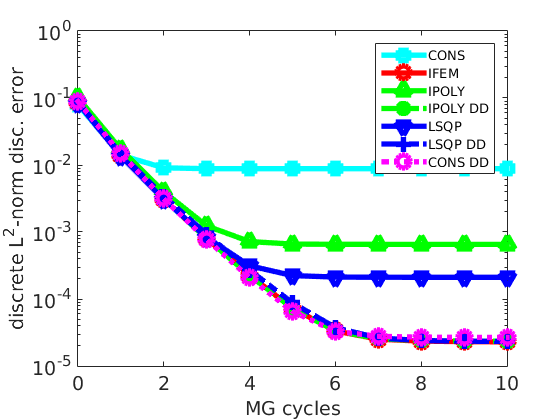
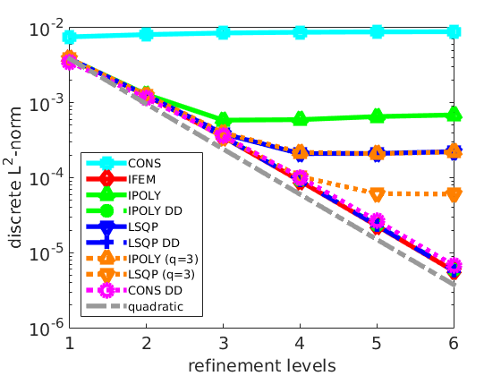
One can see that the discretization error for CONS clearly suffers from the insufficient resolution of the spherical geometry. The errors for IPOLY and LSQP are roughly a factor of 10 and 50 smaller, respectively. We observe that LSQP performs better than IPOLY which can be attributed to a smaller constant in (10). This supports the observation from Sec. 3.2 that the stencils are uniformly better fitted. Note that, as was to be expected for a rather coarse input mesh (large $H$) and multiple refinements (large $L$), the error is dominated by the approximation error in the stencil $s$ introduced by replacing its values by those of the surrogate polynomials. Using the double discretization scheme, however, allows to (almost) recover the discretization error of the IFEM approach. Here, both IPOLY DD and LSQP DD perform equally well and even CONS DD achieves very good results.

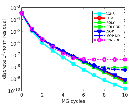
In Fig. 4.3, we provide the discrete $L^{2}$-norms of the residuals. We observe that the convergence for the DD variants breaks down after a few iterations. As already indicated, this was to be expected due to the inconsistency in smoothing and residual computation. Whereas the residuals of all non DD-scenarios show similar asymptotic convergence rates.

In Fig. 4.4, we show the discrete $L^{2}$-error for increasing refinement levels. As expected, IFEM shows quadratic order convergence.

This is also satisfied by the DD approaches. But, as already mentioned before, this does not hold for IPOLY and LSQP. Nevertheless, we observe in the pre-asymptotic regime a second order error decay and only asymptotically, the error is dominated by the term in $H^{q+1}$, see also (11). For LSQP we observe second order for $L\leqslant 3$, while for IPOLY this is only the case for $L\leqslant 2$.

Figure 4.4. Discretization error in discrete $L^{2}$ norm for different levels of refinement.

While DD shows excellent convergence, it also requires the application of the expensive operator $\mathcal{L}_{\ell}$. Although it is used only every seventh operator call, in case of a V(3,3) cycle, it still dominates the time to solution. This can be seen in the scaling results in Sec. 6.

Motivated by the a priori estimates from Sec. 3.5, we further investigate the dependence of LSQP and IPOLY on the refinement level $L$, the macro mesh-size $H$ and the polynomial degree $q$. The above test setting describes the coarsest macro mesh with 60 elements. Further refinement in radial and tangential direction results in input meshes $\mathcal{T}_{-2}$ with 480, 3,840 and 30,720 macro elements, respectively. The discretization error for IFEM, LSQP and IPOLY after 10 multigrid cycles is displayed in Tab. 4.1 for different numbers of macro elements and different polynomial degrees, $q=1,2,3$. These results are for $j=2$ in $m(\ell,j)$, i.e. for $S_{\ell}=M_{2}$. We note that using a computationally more expensive choice of $S_{\ell}$ did not yield any significant differences.

As expected, we see in Tab. 4.1 a quadratic convergence for IFEM. For the other variants we observe that for a finer input mesh and for a higher polynomial degree, the accuracy obtained increases. Combinations for which $e_{\textsc{LSQP}}$ or $e_{\textsc{IPOLY}}$ differ relatively by more than 10 percent from $e_{\textsc{IFEM}}$ are highlighted by italic table entries.

We find that for IPOLY and $q=1$ the maximal feasible refinement level $L$ is independent of $H$. While for $q=2$ two refinements in $H$ allow one more refinement in $L$. And for $q=3$ those values form a diagonal, meaning that for each finer $H$ also $L$ can be increased by one. For LSQP the results look even better. As a rule of thumb we observe that for LSQP the italic entries are shifted by at least one level down compared to IPOLY.

Table 4.1. Discretization error for IFEM and IPOLY/LSQP (linear, quadratic and cubic) for different combinations of $h_{\ell}$ and $H$. Italic entries have a relative deviation from the reference $e_{\textsc{IFEM}}$ of more than 10 percent.

#mac el	60	480	3840	30720
	$e_{\textsc{IFEM}}$
$L=2$	1.2e-03	3.5e-04	8.9e-05	2.2e-05
$L=3$	3.4e-04	9.4e-05	2.2e-05	5.6e-06
$L=4$	9.0e-05	2.3e-05	5.7e-06	1.4e-06
$L=5$	2.2e-05	5.9e-06	1.4e-06	3.5e-07
$L=6$	5.7e-06	1.5e-06	3.5e-07	8.9e-08
	$e_{\textsc{IPOLY}}$ ($q=1$)
$L=2$	1.5e-03	4.1e-04	8.9e-05	2.2e-05
$L=3$	2.1e-03	5.6e-04	1.1e-04	2.8e-05
$L=4$	2.7e-03	7.3e-04	1.5e-04	3.8e-05
$L=5$	3.1e-03	8.2e-04	1.8e-04	4.4e-05
$L=6$	3.3e-03	8.7e-04	1.9e-04	4.7e-05
	$e_{\textsc{IPOLY}}$ ($q=2$)
$L=2$	1.3e-03	3.6e-04	9.0e-05	2.3e-05
$L=3$	5.9e-04	1.0e-04	2.3e-05	5.7e-06
$L=4$	5.9e-04	6.3e-05	6.5e-06	1.5e-06
$L=5$	6.5e-04	6.7e-05	3.4e-06	4.0e-07
$L=6$	6.9e-04	7.1e-05	3.1e-06	1.7e-07
	$e_{\textsc{IPOLY}}$ ($q=3$)
$L=2$	1.3e-03	3.6e-04	9.0e-05	2.3e-05
$L=3$	4.0e-04	9.6e-05	2.3e-05	5.7e-06
$L=4$	2.2e-04	2.7e-05	5.9e-06	1.4e-06
$L=5$	2.1e-04	1.2e-05	1.6e-06	3.7e-07
$L=6$	2.2e-04	9.9e-06	6.4e-07	1.0e-07
	$e_{\textsc{LSQP}}$ ($q=1$)
$L=2$	1.3e-03	3.7e-04	9.0e-05	2.3e-05
$L=3$	7.7e-04	1.4e-04	2.7e-05	6.4e-06
$L=4$	8.0e-04	1.1e-04	1.5e-05	3.1e-06
$L=5$	8.5e-04	1.2e-04	1.4e-05	2.8e-06
$L=6$	8.8e-04	1.2e-04	1.5e-05	2.9e-06
	$e_{\textsc{LSQP}}$ ($q=2$)
$L=2$	1.3e-03	3.6e-04	8.9e-05	2.3e-05
$L=3$	3.9e-04	9.4e-05	2.3e-05	5.7e-06
$L=4$	1.9e-04	2.5e-05	5.6e-06	1.4e-06
$L=5$	1.8e-04	1.3e-05	1.4e-06	3.5e-07
$L=6$	1.9e-04	1.3e-05	3.8e-07	8.2e-08
	$e_{\textsc{LSQP}}$ ($q=3$)
$L=2$	1.3e-03	3.6e-04	8.9e-05	2.3e-05
$L=3$	3.5e-04	9.4e-05	2.3e-05	5.7e-06
$L=4$	1.0e-04	2.4e-05	5.7e-06	1.4e-06
$L=5$	6.9e-05	5.8e-06	1.4e-06	3.5e-07
$L=6$	7.3e-05	1.9e-06	3.3e-07	8.7e-08

These observations confirm our theory that the discretization error is a combination of two parts: one fine scale part $h_{\ell}^{2}$ and one depending on the coarse meshsize $H$, but being of higher order depending on the selected polynomial degree.

Real geophysical applications will typically be executed on HPC systems with ${\mathcal{O}}(10^{5})$ cores. Each core will then manage at least one, but often also more than one macro element, imposing a small upper bound on $H$ and thus a reasonable large bound on $L$. Hence, in these application we will be automatically in an $(L,H)$-parameter regime that does not exceed the critical $L$. Consequently our two-scale approach is perfectly suited for this kind of applications.

4.2. Cost considerations

Besides the quality of the approximation, we also have to consider its cost. We split our considerations into two parts, the cost for applying and the cost for setting up the surrogate operator. While our two approaches IPOLY and LSQP have different setup costs, the cost for the evaluation of the surrogate stencil operator is the same in both surrogate approaches. Moreover once the stencil weights are evaluated, the application of the actual stencil is independent of the chosen approach.

4.2.1. Cost for operator evaluation

To give a quantitative idea Tab. 4.2 provides the number of FLOPs for a single Gauss-Seidel relaxation step, which involves the equivalent of one stencil application, see (13) below. We base our considerations, w.r.t. polynomial evaluation, on the incremental approach. Note that the traditional FLOPs measure can only give an impression on the arithmetic load of the different variants. The actual execution times depend on various implementation details, see also Sec. 5 where we discuss how to optimize the polynomial evaluation with respect to run-time.

For the constant case, we get in Tab. 4.2 the minimal value of 29 FLOPs, as the same pre-computed stencil can be used at all nodes. As mentioned above this cost for the stencil application remains the same in the other approaches. However, the extra cost for computing the proper finite element or surrogate stencil entries occur. As a small detail note that in the constant case HHG employs a multiplication with the reciprocal of the central stencil weight in (13) which gets pre-computed in the setup phase. For the other approaches we need to perform a floating point division, which is more costly.

Setting up the stencil in the IFEM approach with projected coordinates involves firstly computing for the current node the element matrices of its surrounding 24 elements. For this we use a C++ code that was auto-generated and optimized using the FEniCS Form Compiler (FFC), see [33], which results in 53 FLOPs per element matrix. Stencil weights are obtained by summing up the associated entries in the element matrices. In our 15-point-stencil, we have 6 weights belonging to edges attached to 4 neighboring elements and 8 weights belonging to edges attached to 6 neighboring elements, see Fig. 2.3. Hence, computation of the non-central stencil weights adds another 58 FLOPs. The central weight can either be assembled in the same fashion (23 FLOPs) or via the row sum property (13 FLOPs). Altogether this leads to the cost of 1353 resp. 1343 FLOPs given in Tab. 4.2. Thus, this approach is nearly a factor of $50$ more costly than the constant one. Though, to be fair, we remark that our implementation does not take into account the fact that each element matrix is shared by four nodes. However, exploiting this is not straightforward as the point-smoother we are considering here requires an assembled central stencil weight and re-using element matrices for different nodes introduces additional overhead to manage the related dependency information.

Table 4.2. Number of FLOPs for a single stencil application in a Gauss-Seidel relaxation step for a scalar operator in HHG. For fair comparison DD cost is averaged over cheap smoothing and expensive residual computation.

Constant	29
IFEM (direct)	1353
IFEM (row sum)	1343
IPOLY/LSQP (naïve, $q=2$)	378
IPOLY/LSQP (increment)	29+15q
CONS DD	$\frac{1343+29\nu}{\nu+1}$

We now turn to our proposed surrogate stencils. Here we need to add on top of the cost for applying the stencil the evaluation of the polynomials to obtain its weights. If we employ the naïve approach, i.e., a straightforward evaluation with respect to its monomial basis representation, we end up with 378 FLOPs for a tri-variate quadratic polynomial. Here, we assumed the sum rule is employed for the central weight. This already gains a factor of 3.5 compared to IFEM, but still requires over ten times more FLOPs than in the constant case. Now, for the incremental approach, asymptotically, only two operations are needed for the evaluation of each polynomial. Thus, the total number of FLOPs decreases to 59, which is only about twice the optimal value of the constant setting. Note that in this case, evaluation of the central entry via its polynomial is, of course, cheaper than the sum rule. Using higher order polynomials of degree $q$, we asymptotically need $q$ operations and an additional cost factor of

(12) $$C(q)=1+\frac{15q}{29}\approx 1+\frac{q}{2}.$$

So the cubic IPOLY/ LSQP approach, overall, is a factor of 1.25 more expensive than the quadratic one.

To quantify the cost of a CONST double discretization approach in comparison with a pure IPOLY/ LSQP approach ($q=2$), we take the average over one residual computation and a total of $\nu$ pre- and post-smoothing steps. For a typical choice of $\nu$ ranging between 2 and 8 the resulting cost factor is roughly between 8 and 3. This demonstrates that DD is an option that should seriously be considered, but overall is still dominated by the expensive residual computation.

In order to reach the best performance it is better to either decrease $H$ or to increase the polynomial degree. For smaller runs on workstations or on mid-sized clusters the latter may be the preferred choice in order to keep the number of macro elements as low as possible. Whereas for large scale simulation on high performance computers, quadratic polynomials seem most suitable. Here, $H$ is decreased almost naturally as the number of cores that are to be used is coupled to the number of macro elements.

4.2.2. Cost for setup

Table 4.3. Number of sampling points $|S_{L}|$ for a single macro element on finest level $(L=5)$, sum of sampling points over all levels, time $t_{\text{sample}}$ for stencil computation at sampling points, $t_{\text{linalg}}$ for computation of polynomial coefficients, $t_{\text{setup}}$ for total setup, $t_{\text{cycle}}$ for a single V(3,3)-cycle, $p_{\text{cycle}}$ percentage of $t_{\text{setup}}$ w.r.t. $t_{\text{cycle}}$; for IFEM $p_{\text{cycle}}$ relates an IFEM to a LSQP cycle; for LSQP values depend on strategy $m(\ell,j)$ for choosing $S_{\ell}$; times are given in seconds.

	$j$	$|S_{L}|$	$\sum_{\ell=1}^{L}|S_{\ell}|$	$t_{\text{sample}}$	$t_{\text{linalg}}$	$t_{\text{setup}}$	$t_{\text{cycle}}$	$p_{\text{cycle}}$
IPOLY	—	10	50	0.01	0.001	0.01	16.8	0.1%
	$2$	455	1,855	0.52	0.02	0.56	16.8	3%
LSQP	$\ell-1$	39,711	44,731	11.06	0.37	11.53	16.8	67%
	$\ell$	333,375	378,071	96.22	4.10	102.66	16.8	611%
IFEM	—	333,375	378,071	—	—	—	872.8	5195%

We continue by considering the setup phase. This consists in the computation of the sampling values and the solution of the resulting linear systems for IPOLY or least-squares problems for LSQP. For the IPOLY approach with its small number of sampling points and very low dimensional linear system we expect the cost to be negligible. In the LSQP approach, however, the situation might be different as problem size strongly varies with the choice of the sampling set $S_{\ell}$.

To quantify this setup cost we report in Tab. 4.3 on run-times related to the setup phase and compare them to the execution time for a single V(3,3)-cycle with our surrogate operator. For this we restrict ourselves to the case of quadratic polynomials and deliberately consider the worst case scenario of a monomial basis. Measurements were performed for a serial run on a single node on the SuperMUC cluster, cf. Sec. 6 for technical details. The code was compiled with the Intel Compiler version 15.0. Linear systems for IPOLY were solved using the DGESV routine of LAPACK, while for the least-squares problems in the LSQP case we used DGELS. In both cases the LAPACK implementation from the Intel Math Kernel Library (MKL) in version 11.3 was employed. The macro mesh consisted of 60 elements, and we used $L=5$ levels of refinement. Reported values are the minimal ones over a collection of test runs.

Table 4.3 lists the size of the sampling set for the finest level and the total number of sampling points over levels 1 to $L$ for IPOLY and LSQP with different choices for $m(\ell,j)$, see (8). The value $t_{\text{sample}}$ represents the time spent with computing stencil weights at the sampling points from the finite element formulation with projected coordinates. This was performed as described in Sec. 4.2.1 for the IFEM approach. The values $t_{\text{linalg}}$ and $t_{\text{setup}}$ give the time required for the solution of the linear systems resp. least-squares problems and the total time of the setup phase for computing the polynomial coefficients. The last two columns provide information to relate the cost of the setup to those for the evaluation and application of our surrogate operator. $t_{\text{cycle}}$ represents the run-time for a single $V(3,3)$–cycle using, in the case of IPOLY and LSQP, the surrogate operator and $p_{\text{cycle}}$ gives the percentage of $t_{\text{setup}}$ with respect to $t_{\text{cycle}}$.

For comparison the last row shows for the IFEM approach the number of sampling points, the cost for a $V(3,3)$–cycle using this operator and percentage of these cost compared to $t_{\text{cycle}}$ of the surrogate operator. Remember that in this approach there is no setup phase, but instead the stencils are re-computed on-the-fly for each stencil application. This must be done for every node which corresponds to LSQP using $j=\ell$.

Examining the results we see that, as expected, the cost for IPOLY is marginal, only 0.1% of the time required for a single V(3,3)-cycle. This changes dramatically, when we employ for LSQP all available points $\mathcal{M}_{\ell}$ on level $\ell$ as sampling points, i.e.,  we choose $j=\ell$ for $m(\ell,j)$. However, already for $j=(\ell-1)$ this reduces to 67%, i.e., two thirds of one multigrid cycle. For $m(\ell,j)\equiv 2$ this reduces further to only 3% and this choice seems to be the optimal trade-off between accuracy and cost. We point out that the relative cost is measured with respect to one MG-cycle based on the surrogate operator evaluation.

Note that for all choices in the LSQP case the majority, between 90 and 95%, of the time for the setup phase is spent in the evaluation of the stencil weights at the sampling points and only the remaining fraction is required for solving the least-squares problems.

Our previous accuracy experiments had shown that even using a sampling set $S_{\ell}$ as coarse as $M_{2}$ can give satisfactory results and thus the relative setup cost for our surrogate approaches is quite small compared to the total cost of the solver.

5. Kernel optimization

In Sec. 4, the run-time $t_{\text{cycle}}$ of a single V-cycle was measured in a serial setting. Comparing the measured 16.8 seconds to the 5.0 seconds required for a V-cycle with a constant stencil application shows that our straightforward implementation based on incremental polynomial evaluation underperforms. We exceed the theoretically expected cost factor given in (12) by roughly a factor of 1.68.

Thus we now focus on a node-level performance analysis and a more sophisticated re-implementation of the surrogate polynomial application. As we are mainly interested in extreme scale simulations, this will be done for the quadratic case.

In the following, we study the optimization of the GS smoother in detail. Updating the value of the current iterative solution at node $I$ can be formulated as

(13) $$\mathbf{u}_{I}=\frac{1}{s_{mc}^{I}}\left(\mathbf{f}_{I}-\sum_{w\in\mathcal{W}\setminus\{mc\}}s_{w}^{I}\mathbf{u}_{I_{w}}\right)$$

and, naturally, involves all 15 stencil weights $s_{w}^{I}$. Here $I_{w}$ stands for the node which is the closest one to $I$ when we move in direction $w$. We will refer to this as a stencil-based update (SUP) below.

Our Gauss-Seidel smoother uses a lexicographic ordering. Within HHG this implies that the function values $\mathbf{u}_{I}$ are updated in the following ordering, as shown in Fig. 2.4. We traverse the nodes of a volume primitive from west to east, going line by line from south to north and plane by plane from bottom to top. Hence, when updating the value at node $I$, the values at the neighboring nodes with indices $bc$, $be$, $bnw$, $bn$, $ms$, $mse$, and $mw$ have already been updated during the current sweep, whereas values at nodes with indices $me$, $mnw$, $mn$, $ts$, $tse$, $tw$, and $tc$ still need to be updated. Note that due to the hybrid nature of the smoother this is true for the majority of, but not for all nodes, as those near the boundary couple to lower dimensional primitives. Consequently, the only data dependency which must be considered during the update inside a line is $\mathbf{u}_{I_{mw}}$. This value is only available for updating $\mathbf{u}_{I}$ after the update at the previous node, i.e., $I_{mw}$, was computed. We further remark that due to the lexicographic ordering, the $tc$ value is the only one that has not been touched in a previous update. Hence, it has not been loaded into the cache so far.

Our analysis revealed that the recursive dependency in  (13) dominates the execution time for the update. Furthermore, it hinders certain optimizations, like vectorization, and thereby prohibits exploiting the full floating point performance of the core.

To circumvent this problem, the update formula (13) for all nodes within one line of the volume primitive is re-arranged. For this, we split it into a non-recursive and a recursive part $\mathbf{u}_{I}=\tau+\rho$ with

(14) $$\tau =\frac{1}{s_{mc}^{I}}\Big{(}\mathbf{f}_{I}-\sum_{\begin{subarray}{c}w\in\mathcal{W}\\ w\notin\{mc,mw\}\end{subarray}}s_{w}^{I}\mathbf{u}_{I_{w}}\Big{)}$$

(15) $$\rho =-\frac{1}{s^{I}_{mc}}s^{I}_{mw}\mathbf{u}_{I_{mw}}\enspace.$$

Firstly, the non-recursive part $\tau$ is pre-computed and stored in a temporary array, tmp in Alg. 1 below, large enough to hold the results for a complete line. As an incremental polynomial evaluation does not allow complete vectorization, we instead represent the stencil weights $s^{d}_{w}$ for $d\in\mathbb{N}_{0}$ as

(16) $$s^{d}_{w}=\hat{p}_{w}(0)+d\,\delta\hat{p}_{w}(0)+\frac{(d-1)d}{2}\delta k_{w}$$

with $\hat{p}_{w}(0):={\mathcal{P}}^{\alpha}s_{w}(0,j_{0},k_{0})$ and

$$\begin{split}\delta\hat{p}_{w}(0)&:=\left.\frac{d{\mathcal{P}}^{\alpha}s_{w}(i,j_{0},k_{0})}{di}\right|_{i=0}+\frac{\delta k_{w}}{2}\,,\\ \delta k_{w}&:=\left.\frac{d^{2}{\mathcal{P}}^{\alpha}s_{w}(i,j_{0},k_{0})}{di^{2}}\right|_{i=0}\,.\end{split}$$

Here, the index $d$ denotes the position of a node inside the current line, starting at 0. For the very first line, the values $\hat{p}_{w}(0)$, $\delta\hat{p}_{w}(0)$ and $\delta k_{w}$ have to be initialized. For all further lines even these values are obtained by updates analogue to (16) in $j$ or $k$ direction, respectively.

For performance reasons, (14) is further split into two loops, where in the first all stencil elements in $\mathcal{W}_{1}$ are treated and then those in $\mathcal{W}_{2}$. The two sets are defined as

$$\mathcal{W}_{1} =\{me,mnw,mn,ts,tse,tw\},$$

$$\mathcal{W}_{2} =\{tc,bc,be,bnw,bn,ms,mse\}.$$

On the tested architecture, see below, this splitting avoids problems with register spilling, see e.g. [34]. The distribution of the sets is based on hardware dependent performance investigations as detailed in Sec. 5.1 and has no geometric meaning.

Now in a second step, the recursive part $\rho$, see (15), is computed and the stencil update completed by combining it with the pre-computed value $\tau$ stored in the temporary array. Unrolling this last loop by a factor of four or eight increases the performance on the evaluated hardware architecture.

The full pseudo code for the optimized GS smoother is displayed in Alg. 1.

1:  for line $(k,j,0:n-1)\in$ TET do

2:     initialize/update $s_{w}^{0}$, $\delta\hat{p}_{w}^{0}$

3:     // setup stencils along line and store in tmp array tmp[d], tmp_mw[d], and tmp_mc[d], except recursive part mw.

4:     for d = 0, … n-1 do // loop 1: vectorized

5:        tmp[d] = $f^{d}$; tmp_mc[d] = 0

6:        for $w_{1}\in\mathcal{W}_{1}$ do // completely unrolled

7:           compute stencil weight $s_{w_{1}}$ // evaluate (16)

8:           tmp[d] -= $s^{d}_{w_{1}}\times u^{d}_{w_{1}}$, tmp_mc[d] -= $s^{d}_{w_{1}}$

9:        end for

10:     end for

11:     for d = 0, … n-1 do // loop 2: vectorized

12:        for $w_{2}\in\mathcal{W}_{2}$ do // completely unrolled

13:           compute stencil weight $s^{d}_{w_{2}}$ // evaluate (16)

14:           tmp[d] -= $s^{d}_{w_{2}}\times u^{d}_{w_{2}}$, tmp_mc[d] -= $s^{d}_{w_{2}}$

15:        end for

16:        compute stencil weight $s^{d}_{mw}$ // evaluate (16)

17:        tmp_mc[d] -= $s^{d}_{mw}$, s0 = 1 / tmp_mc[d]

18:        tmp_mw[d] = s0 $\times s^{d}_{mw}$, tmp[d] = tmp[d] $\times$ s0

19:     end for

20:     // compute recursive part to finish application of the stencil(s)

21:     for d = 0, … n-1 do // loop 3: 4- or 8-way unrolled

22:        $u^{d}_{mc}$ = tmp[d] - tmp_mw[d] $\times$ $u^{d}_{mw}$

23:     end for

24:  end for

Algorithm 1 optimized GS smoother

5.1. Single core performance

In the following, we will conduct a detailed performance investigation. This will be based on performance modeling and compared to actual measurements. Note that we do not include the initialization in line 2 of the algorithm and that the setup phase for computing the polynomials representing the weights of our surrogate operator is considered neither in the model nor in the measurements. The latter is justifiable as for reasonable choices of $m(\ell,j)$ the cost is negligible.

Benchmarked system

The execution is modeled for and evaluated on the Haswell based Intel Xeon E5-2695 processor with $14$ cores, which was configured in cluster on die mode, i. e. seven cores per NUMA domain. This is the same system as used in the SuperMUC Phase $2$ cluster, on which the scaling experiments of Sec. 6 were conducted. The only difference is that the processor here was only clocked at $2.3$ GHz instead of $2.6$ GHz on the SuperMUC.

One core of the Intel Xeon comprises several execution ports, which can perform: floating point (FP) multiply & FP fused multiply add (FMA), FP addition & FP FMA, FP division, load, and store. Transferring a cache line between L1/L2 cache or L2/L3 cache takes $2$ cycles (cy) on Haswell, respectively. As the system sustains $24.2$ GiB/s memory bandwidth from one NUMA domain, it takes $5.7$ cy at $2.3$ GHz to transfer one cache line between L3 cache and memory.

Performance modeling

Our performance analysis is based on the Execution–Cache–Memory (ECM) model [35]. In contrast to the simpler Roofline model [36], which only takes into account the (number of) floating point operations performed for a certain amount of data transferred between core and memory, the ECM model considers the complete path of the memory hierarchy including caches. Furthermore the complete execution inside the core is examined, which, besides floating point operations, includes also, e.g., address generation and register spilling. As in the actual memory hierarchy, data is transferred in the granularity of cache lines, the modeling is based on this unit. On the target architecture a cache line comprises $64$ bytes, which is for the stencil considered equivalent to eight updates. In the following, the modeling of the execution and the data transfers inside the memory hierarchy are outlined.

Table 5.1. Cycle numbers reported by IACA for the three loops normalized to eight stencil-based updates. Given are the maximum values for each execution unit of a certain category. The reported duration of $40$ cy from IACA for loop 3 is higher than the occupancy of the execution ports. This is due to the data dependencies, which hinder efficient instruction pipelining.

		max		FP division	FP mul	FP add		load	store
loop 1		22		0	20	20		22	2
loop 2		56		56	32	34		36	4
loop 3		40		0	4	4		12	8

Modeling of execution

For modelling the execution of the optimized implementation inside the core, the Intel Architecture Code Analyzer (IACA) is used, see [37]. The tool generates a scheduling of the instructions over the available execution ports on a certain micro-architecture for a given binary. This was also used to derive the optimal distribution of the two sets $\mathcal{W}_{1}$ and $\mathcal{W}_{2}$. Here it is assumed that all data can be fetched from L1 data cache. IACA can operate in two modes: throughput and latency. In throughput mode it is assumed that the considered loop iterations are independent and can overlap, while in latency mode, it is assumed that operations between iterations cannot overlap. Analyzing the three loops in our implementation with throughput mode resulted in the closest agreement of prediction and measurement.

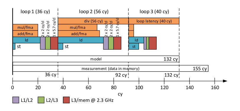
The values reported by IACA for eight stencil-based updates, our base unit from above, on the Haswell micro-architecture are listed in Tab. 5.1 for the two vectorized loops (loop 1 and 2) as well as the loop containing the recursive component (loop 3). To ease the modeling process the initialization and setup of the stencil weights in line $2$ of Alg. 1 are not considered. Whereas loop 1 and 2 are limited by the occupancy of the execution ports, IACA reports for loop 3 as bottleneck the loop latency with 40 cy. This indicates that due to data dependencies resulting from the recursion in loop 3 instructions cannot be fully pipelined and stall until their corresponding operands become available.

A more detailed overview is presented in Fig. 5.1 which displays the occupancy of the execution units.

Modeling of cache and memory transfers

The amount and duration of cache line transfers inside the memory hierarchy for eight stencil-based updates beyond L1 data cache are modeled manually. Those numbers depend on the refinement level $\ell$ of the macro tetrahedron, as it determines how many data items can be re-used from cache. If two planes of the tetrahedron fit concurrently into a cache level, i.e., the so called layer condition [38] is fulfilled, then only the leading stencil neighbor $u^{I}_{tc}$ must be loaded from a higher cache level, the last stencil neighbor $u^{I}_{bc}$ gets evicted, and the remaining neighbors can be fetched from this cache level. In our case, we focus on $\ell=5$ and for simplicity consider the case where the layer condition is only fulfilled in L3 cache. For L1 and L2 cache we assume, that in each cache level only six rows of the tetrahedron, i.e., two rows from top, middle, and bottom plane each, can be kept concurrently.

With this assumptions between L1/L2 cache and L2/L3 cache five cache lines are transferred, respectively: one cache line from each plane containing $u^{I}_{tc}$, $u^{I}_{mn}$, and $u^{I}_{bn}$ is loaded (three loads), one cache line containing the corresponding element from the $f$ array (one load), and the modified cache line containing $u^{I}_{mc}$ gets evicted (one store). As in L3 cache the layer condition is fulfilled, instead of three cache lines only the one for the top plane containing $u^{I}_{tc}$ must be loaded (one load). Everything else stays the same, which results in three cache line transfers. Concerning the arrays used for vectorization to store the temporary results, they are small enough to fit with the other data into L1 cache. Further the least recently used cache policy, commonly used on current architectures, ensures that they get not evicted.

Results

The timings resulting from the IACA analysis combined with the manual modeling of the data transfers in the memory hierarchy are summarized in Fig. 5.1. Note that this does not show an exact scheduling of the different execution phases and only sums up the duration of the different parts, which are involved during execution. The predicted duration of $132$ cy for eight stencil-based updates by the ECM model is $\approx 15$% off from the measurement of the executed kernel.

Figure 5.1. Duration of the different phases involved during eight stencil-based updates as obtained by the ECM model. Shown are the durations of executing loop 1, 2, and 3, as well as the time spend with cache line transfers inside the memory hierarchy. For the loops the occupancy of the different execution ports are shown: multiplication/fused multiply add (mul/fma), addition/fused multiply add (add/fma), division (div), loads (ld), stores (st). Considered in neither model nor measurement is the setup of the initial stencil weights.

5.2. Socket performance

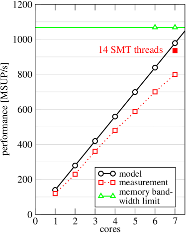
When increasing the core count the ECM model assumes that only shared resources can become a bottleneck. In the case of the benchmarked Haswell system this concerns the segmented L3 cache and the memory interface. However, the bandwidth of the L3 cache scales linearly with the number of cores. Thus, only the memory interface could limit performance. Consequently the performance should increase linearly with the number of cores up to the point where the memory interface becomes continuously occupied. The model prediction and the corresponding measurement are both shown in Fig. 5.2. The code does not saturate the memory bandwidth (green line with triangles) completely. This upper limit is given as ratio of the achievable memory bandwidth of $24.2$ GiB/s with the bytes transferred between L3 and memory required for one stencil-based update. If the layer condition is fulfilled in L3 cache one stencil-based update requires 24 bytes: load of $u^{I}_{tc}$, load of one element from $f$ array, and eviction of updated $u^{I}_{mc}$. Utilizing also the SMT thread of each core (single filled red square) increases performance slightly. This has two reasons. Firstly the memory interface is not continuously utilized and secondly still execution resources on each core are available. The resources are available because of pipeline bubbles, i.e., time slots with no operation in the execution pipeline, due to the division in loop $2$ and the recursion in loop $3$.

Figure 5.2. Performance of the optimized code (in MSUP/s, mega stencil-based updates per second) compared with the ECM model prediction.

6. Weak and strong scaling

Figure 6.1. Run-times of one V(3,3)-cycle. (Left) Weak scaling on SuperMUC. 16 macro elements are assigned to one core. The finest grid is fixed to $L=5$, i.e. there are $3.3\cdot 10^{5}$ DOFs per volume primitive. (Right) Strong scaling (solid) and parallel efficiency (dashed). The problem size is fixed to 12,960 macro elements and $L=5$. In total there are $4.5\cdot 10^{9}$ DOFs.

To demonstrate the performance and scalability of our approach, we perform weak and strong scaling runs on the supercomputer SuperMUC (Phase 2) that is ranked number 28 in the June 2016 TOP500 list. It is a Lenovo NeXtScale system with a theoretical peak performance of 3.58 PFLOPs/s. Each compute node consists of two Haswell Xeon E5-2697 v3 processors where each processor is equipped with 14 cores running at 2.6 GHz. Per core 2.3 GiB of memory are provided, but typically only 2.1 GiB are available for applications. The nodes are connected via an Infiniband (FDR14) non-blocking tree.

For our runs we utilize the Intel C/C++ Compiler 15.0 with flags -O3 -CORE-AVX2 -fma and the Intel MPI library 5.0

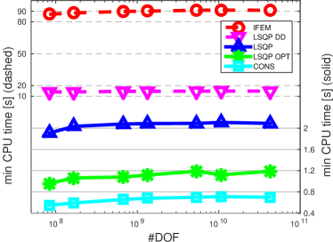
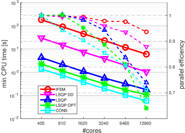
As mentioned before degree two polynomials for the IPOLY/LSQP approach provide the most efficient compromise between accuracy and computational cost in the HPC context. In Fig. 6.1 we present the run-times of one V(3,3)-cycle for the different implementations. For reproducibility we take the minimum value out of ten cycles reflecting the best exploitation of the machine’s capabilities.

The CONS setting serves as minimal cost reference. IPOLY and LSQP differ only in the setup phase, so only LSQP is considered here. For this approach, we compare the straightforward implementation of the method with the optimized version from Sec. 5 termed LSQP OPT. To demonstrate the cost of a conventional assembly of the stencils also the IFEM case is shown. Furthermore the run-times for double discretization are given. Here the non-optimized LSQP implementation is chosen for the smoother and the conventional stencil assembly for residual. As this is dominated by the expensive residual, employing the optimized smoother does not lead to a significant improvement.

For the weak scaling, Fig. 6.1 (left), we assign 16 macro elements to one core and fix the refinement level to $L=5$ giving us $3.3\cdot 10^{5}$ DOFs per volume primitive. The number of macro elements and cores varies from 240 to 122,880 and from 15 to 7,680, respectively.

We observe that the IFEM method is even more expensive than the theoretical prediction from Tab. 4.2 indicated. This is due to additional memory accesses and function calls which are not considered in the flop count. The double discretization is about a factor of 7 slower than the non-optimized LSQP method. This is in line with the flop count for a V(3,3)-cycle taking into account the aforementioned additional cost for the residual. The values for the straightforward implementation of the LSQP method reflect the serial run-time factor of $(1.68\cdot C(2))$ mentioned in Sec. 5. Our optimized version outperforms the cost factor $C(2)\approx 2$, and the run-time increases by only a factor of $1.6$ compared to the CONS case. Also it shows excellent weak scaling behavior.

For the strong scaling case, Fig. 6.1 (right), we fix the problem size to 12,960 macro elements and set $L=5$. In total this results in $4.5\cdot 10^{9}$ DOFs. This also gives an upper bound for the number of cores that can be used. The lower bound is determined by the available memory of 2.1 GiB per core where we need about 100 bytes per DOF in our implementation.

Not surprisingly, the IFEM implementation shows the best parallel efficiency of above 90% even for the largest number of cores. Here, most of the time is spent with the cost intense on-the-fly stencil computation. Thus, increasing the amount of communication by increasing the number of cores does hardly affect the performance that scales almost linearly with the number of cores. This is also the case for the DD approach. Even though the computationally expensive residual occurs a factor of 7 less often then in the IFEM case, it is still the dominating factor. Whereas for the CONS and for the LSQP implementations where the stencil is either already known or computed by an inexpensive evaluation of the surrogate polynomials, we clearly see the influence of communication for the runs with larger number of cores. But nevertheless the run-time even for the largest case of the optimized LSQP method is a factor of 10 or 55 faster than LSQP DD or IFEM, respectively, and only 1.8 times slower than the CONS reference. We point out that for the DD approaches, the expensive operator need only be used in the final few iterations and thus its cost within the solver can be further reduced.

7. Conclusion and outlook

We introduced a novel two-scale approach for handling non-polyhedral domains in large scale simulations with matrix-free finite elements. It is based on replacing the cost intensive on-the-fly computations of the node stencil by the evaluation of a surrogate approximation polynomial of low order. Typically for large system size, second order polynomials already guarantee high enough accuracy and thus reduce the flop counts significantly. This technique can be combined for a further improvement of the numerical accuracy with the classical double discretization approach. Here the smoother in the multigrid algorithm employs cheap lower order stencils while the expensive high accuracy operators are only used to compute the residual for the coarse grid correction.

The accuracy of our approach was first examined theoretically by an a priori estimate and secondly verified by numerical experiments. The implementation was further optimized on the node-level and systematically analyzed by the ECM model. Excellent performance and scalability was demonstrated on the supercomputer SuperMUC. Although all our examples referred to the spherical shell, this approach is completely local with respect to the macro elements and open to general blending functions.

Future work will include different partial differential equations such as the Stokes system, variable coefficients in the PDE and alternative stencil approximations preserving symmetry for $\widetilde{\mathcal{L}}$.

Acknowledgements

This work was partly supported by the German Research Foundation through the Priority Programme 1648 ”Software for Exascale Computing” (SPPEXA) and by WO671/11-1. The authors gratefully acknowledge the Gauss Centre for Supercomputing (GCS) for providing computing time on the supercomputer SuperMUC at Leibniz-Rechenzentrum (LRZ).

References

- [1] J.A. Cottrell, T.J.R. Hughes, and Y. Bazilevs. Isogeometric Analysis: Towards Integration of CAD and FEA. John Wiley Sons, Ltd., 2009.
- [2] Y. Bazilevs, K. Takizawa, and T.E. Tezduyar. Computational Fluid-Structure Interaction: Methods and Applications. John Wiley Sons, Ltd., 2013.
- [3] Brian L. N. Kennett and Hans-Peter Bunge. Geophysical Continua. Cambridge University Press, 2008.
- [4] Heiner Igel. Computational Seismology: A Practical Introduction. Oxford University Press, 2016.
- [5] R. Barrett, M. Berry, T. F. Chan, J. Demmel, J. Donato, J. J. Dongarra, V. Eijkhout, R. Pozo, C. Romine, and H. van der Vorst. Templates for the Solution of Linear Systems: Building Blocks for Iterative Methods. SIAM, 1994.
- [6] M. Kreutzer, G. Hager, G. Wellein, H. Fehske, and A. Bishop. A Unified Sparse Matrix Data Format for Efficient General Sparse Matrix-Vector Multiplication on Modern Processors with Wide SIMD Units. SIAM J. Sci. Comput., 36(5):C401–C423, 2014.
- [7] Dahai Guo, William Gropp, and Luke N Olson. A hybrid format for better performance of sparse matrix-vector multiplication on a GPU. International Journal of High Performance Computing Applications, 30(1):103–120, 2016.
- [8] Steven Dalton, Luke Olson, and Nathan Bell. Optimizing Sparse Matrix-Matrix Multiplication for the GPU. ACM Trans. Math. Softw., 41(4):25:1–25:20, 2015.
- [9] Amanda Bienz, Robert Falgout, William Gropp, Luke Olson, and Jacob Schroder. Reducing parallel communication in algebraic multigrid. SIAM Journal on Scientific Computing (2015),, 2015. in review.
- [10] Craig C Douglas, Jonathan Hu, Markus Kowarschik, Ulrich Rüde, and Christian Weiß. Cache optimization for structured and unstructured grid multigrid. Electronic Transactions on Numerical Analysis, 10:21–40, 2000.
- [11] Markus Kowarschik, Ulrich Rüde, and Christian Weiß. Data layout optimizations for variable coefficient multigrid. In International Conference on Computational Science, volume 2331 of Lecture Notes in Computer Science, pages 642–651. Springer, 2002.
- [12] Bert van Rietbergen, Harrie Weinans, Rik Huiskes, and Ben Polman. Computational strategies for iterative solutions of large fem applications employing voxel data. International Journal for Numerical Methods in Engineering, pages 2743–2767, 1996.
- [13] B. Bergen and F. Hülsemann. Hierarchical hybrid grids: data structures and core algorithms for multigrid. Numer. Linear Algebra Appl., 11:279–291, 2004.
- [14] Peter Arbenz, G Harry van Lenthe, Uche Mennel, Ralph Müller, and Marzio Sala. A scalable multi-level preconditioner for matrix-free -finite element analysis of human bone structures. International Journal for Numerical Methods in Engineering, 73(7):927–947, 2008.
- [15] M. Kronbichler and K. Kormann. A generic interface for parallel cell-based finite element operator application. Computers and Fluids, 63:135–147, 2012.
- [16] D. A. May, J. Brown, and L. Le Pourhiet. A scalable, matrix-free multigrid preconditioner for finite element discretizations of heterogeneous Stokes flow. Computer Methods in Applied Mechanics and Engineering, 290:496––523, 2015.
- [17] A. Baker, R. Falgout, T. Kolev, and U. Meier Yang. High-Performance Scientific Computing – Algorithms and Applications, chapter Scaling Hypre’s Multigrid Solvers to 100,000 Cores, pages 261–279. Springer, 2012.
- [18] Allison H. Baker, Axel Klawonn, Tzanio Kolev, Martin Lanser, Oliver Rheinbach, and Ulrike Meier Yang. Scalability of classical algebraic multigrid for elasticity to half a million parallel tasks. In Software for Exascale Computing – SPPEXA 2013–2015. Springer, 2016. to appear.
- [19] P. Bastian, M. Blatt, A. Dedner, C. Engwer, R. Klöfkorn, R. Kornhuber, M. Ohlberger, and O. Sander. A generic grid interface for parallel and adaptive scientific computing. Part ii: Implementation and tests in DUNE. Computing, 82(2-3):121–138, 2008.
- [20] Peter Bastian, Christian Engwer, Dominik Göddeke, Oleg Iliev, Olaf Ippisch, Mario Ohlberger, Stefan Turek, Jorrit Fahlke, Sven Kaulmann, Steffen Müthing, and Dirk Ribbrock. EXA-DUNE: Flexible PDE Solvers, Numerical Methods and Applications, pages 530–541. Springer International Publishing, Cham, 2014.
- [21] R. Falgout and U. Meier-Yang. hypre: A library of high performance preconditioners. Computational Science-ICCS 2002, pages 632–641, 2002.
- [22] Yvan Notay and Artem Napov. A massively parallel solver for discrete Poisson-like problems. J. Comput. Phys., 281(C):237–250, January 2015.
- [23] J. Bielak, O. Ghattas, and E.-J. Kim. Parallel Octree-Based Finite Element Method for Large-Scale Earthquake Ground Motion Simulation. Computer Modeling in Engineering & Sciences, 10:99–112, 2005.
- [24] C. Burstedde, G. Stadler, L. Alisic, L. C. Wilcox, E. Tan, M. Gurnis, and O. Ghattas. Large-scale adaptive mantle convection simulation. Geophys. J. Internat., 192(3):889–906, 2013.
- [25] Johann Rudi, A. Cristiano I. Malossi, Tobin Isaac, Georg Stadler, Michael Gurnis, Peter W. J. Staar, Yves Ineichen, Costas Bekas, Alessandro Curioni, and Omar Ghattas. An extreme-scale implicit solver for complex pdes: Highly heterogeneous flow in earth’s mantle. In Proceedings of the International Conference for High Performance Computing, Networking, Storage and Analysis, SC ’15, pages 5:1–5:12, New York, NY, USA, 2015. ACM.
- [26] A. Brandt and O.E. Livne. Multigrid Techniques: 1984 Guide with Applications to Fluid Dynamics, Revised Edition. Classics in Applied Mathematics. Society for Industrial and Applied Mathematics, 2011.
- [27] J. Bey. Tetrahedral grid refinement. Computing, 55(4):355–378, 1995.
- [28] B. Flemisch, J. M. Melenk, and B. I. Wohlmuth. Mortar methods with curved interfaces. Appl. Numer. Math., 54(3-4):339–361, 2005.
- [29] Benjamin Bergen. Hierarchical Hybrid Grids: Data Structures and Core Algorithms for Efficient Finite Element Simulations on Supercomputers. PhD thesis, Technische Fakultät der Friedrich-Alexander-Universität Erlangen-Nürnberg, 2005.
- [30] B. Gmeiner, U. Rüde, H. Stengel, C. Waluga, and B. Wohlmuth. Performance and Scalability of Hierarchical Hybrid Multigrid Solvers for Stokes Systems. SIAM J. Sci. Comput., 37(2):C143–C168, 2015.
- [31] Alyn P. Rockwood. Generalized scanning technique for display of parametrically defined surfaces. IEEE Comput. Graph. Appl., 7(9):15–26, August 1987.
- [32] Ari Rappoport. Rendering curves and surfaces with hybrid subdivision and forward differencing. ACM Trans. Graph., 10(4):323–341, October 1991.
- [33] A. Logg, K. B. Ølgaard, M. E. Rognes, and G. N. Wells. FFC: the FEniCS Form Compiler. In A. Logg, K.-A. Mardal, and G. N. Wells, editors, Automated Solution of Differential Equations by the Finite Element Method, volume 84 of Lecture Notes in Computational Science and Engineering, chapter 11, pages 227–238. Springer, 2012.
- [34] D. E. Comer. Essentials of Computer Architecture. Pearson Prentice Hall, New Jersey, 2005.
- [35] Georg Hager, Jan Treibig, Johannes Habich, and Gerhard Wellein. Exploring performance and power properties of modern multicore chips via simple machine models. Concurrency and Computation: Practice and Experience, 2014.
- [36] Samuel Williams, Andrew Waterman, and David Patterson. Roofline: an insightful visual performance model for multicore architectures. Commun. ACM, 52(4):65–76, Apr 2009.
- [37] Intel Corp. Intel Architecture Code Analyzer. http://software.intel.com/en-us/articles/intel-architecture-code-analyzer, 2012. Version: 2.1.
- [38] Holger Stengel, Jan Treibig, Georg Hager, and Gerhard Wellein. Quantifying performance bottlenecks of stencil computations using the execution-cache-memory model. In Proceedings of the 29th International Conference on Supercomputing, ICS ’15, pages 207–216, New York, NY, USA, 2015. ACM.