Non-LTE line formation of Fe in late-type stars – III. 3D non-LTE analysis of metal-poor stars

Abstract

As one of the most important elements in astronomy, iron abundance determinations need to be as accurate as possible. We investigate the accuracy of spectroscopic iron abundance analyses using archetypal metal-poor stars. We perform detailed 3D non-LTE radiative transfer calculations based on 3D hydrodynamic stagger model atmospheres, and employ a new model atom that includes new quantum-mechanical neutral hydrogen collisional rate coefficients. With the exception of the red giant HD122563, we find that the 3D non-LTE models achieve Fe i/Fe ii excitation and ionization balance as well as not having any trends with equivalent width to within modelling uncertainties of $0.05\,\mathrm{dex}$, all without having to invoke any microturbulent broadening; for HD122563 we predict that the current best parallax-based surface gravity is overestimated by $0.5\,\mathrm{dex}$. Using a 3D non-LTE analysis, we infer iron abundances from the 3D model atmospheres that are roughly $0.1\,\mathrm{dex}$ higher than corresponding abundances from 1D marcs model atmospheres; these differences go in the same direction as the non-LTE effects themselves. We make available grids of departure coefficients, equivalent widths and abundance corrections, calculated on 1D marcs model atmospheres and horizontally- and temporally-averaged 3D stagger model atmospheres.

1 Introduction

Iron is one of the most important elements in astronomy. The high binding energy of ${}^{56}\text{Fe}$ makes it the end product of nucleosynthesis in the cores of massive stars (e.g. Woosley et al., 2002), as well as the main product of Type-Ia supernovae through the radioactive decay of ${}^{56}\text{Ni}$ (e.g. Woosley & Weaver, 1986). Consequently, iron is highly abundant in the cosmos ($\log{\epsilon_{\mathrm{Fe\odot}}}\approx 7.47$ in the solar photosphere; Scott et al., 2015); this, coupled with its rich electronic structure, leads to numerous iron spectral lines that are easy to detect, even in extremely metal-poor stars (e.g. Yong et al., 2013; Sneden et al., 2016). Abundance ratio relations of the form $\mathrm{\left[X/Fe\right]}$ against $\mathrm{\left[Fe/H\right]}$ are commonly used to interpret the chemical evolution of galaxies (e.g. Tinsley, 1979; Edvardsson et al., 1993; Kobayashi et al., 2006). Numerous neutral iron lines with different strengths and atomic properties can be used to constrain the effective temperature $T_{\mathrm{eff}}$ (excitation balance) and microturbulent broadening parameter $\xi$ needed in 1D spectroscopic analyses, while the presence of singly ionized lines also allows constraints on the surface gravity $\log{g}$ (ionization balance; e.g. Bergemann et al., 2012). Finally, as abundances and opacities are interlinked, accurate iron abundances are important for stellar interior modelling: enhanced iron opacities helped to explain the discrepancies between theoretical and observed period ratios of Cepheid variables (Iglesias & Rogers, 1991; Moskalik et al., 1992), and might similarly lead to a resolution of the solar modelling problem (e.g. Serenelli et al., 2009; Bailey et al., 2015).

However, in classical abundance analyses, the accuracy of iron abundance determinations is limited by the assumption of Saha-Boltzmann energy partitioning, or local thermodynamic equilibrium (LTE). There is a rich literature on the non-LTE effects in iron in late-type stars (e.g. Tanaka, 1971; Athay & Lites, 1972; Steenbock, 1985; Takeda, 1991; Thévenin & Idiart, 1999; Gehren et al., 2001a; Gehren et al., 2001b; Korn et al., 2003; Collet et al., 2005; Mashonkina et al., 2011; Bergemann et al., 2012; Lind et al., 2012; Sitnova et al., 2015), with a general consensus that neutral iron suffers from overionization (e.g. Hubeny & Mihalas, 2014, Chapter 14). Qualitatively, non-local radiation originating from deep within the stellar atmosphere drives an underpopulation of the lower levels of the minority Fe i species with respect to LTE in the line-forming regions, and hence a weakening of the Fe i lines. The non-LTE effects are enhanced by the overexcitation of low-lying states ($\lesssim 2\,\mathrm{eV}$) to intermediate states (2 – 5 eV), that are more susceptible to overionization (Bergemann et al., 2012; Lind et al., 2012). The populations of the majority Fe ii species are only slightly perturbed, and therefore non-LTE effects on Fe ii lines are usually insignificant.

One of the main sources of uncertainty in non-LTE investigations stems from how neutral hydrogen collisions are treated (e.g. Asplund, 2005). In the absence of detailed quantum-mechanical calculations, authors have typically either neglected such transitions, or have resorted to the semi-empirical recipe of Drawin (1968, 1969) as formulated by either Steenbock & Holweger (1984) or Lambert (1993), and parametrized with a collisional efficiency scaling factor $S_{\mathrm{H}}$. As discussed in Barklem et al. (2011) and Barklem (2016a), both of these approaches can be prone to severe systematic errors. Non-LTE investigations, in addition to detailed quantum-mechanical calculations for the collisional cross-sections, are necessary for quantifying these errors.

As well as the assumption of LTE, classical abundance analyses are characterized by their use of theoretical one-dimensional (1D) hydrostatic model atmospheres. Real model atmospheres are three-dimensional (3D) and dynamic, and the mean temperature stratification is influenced by the competing effects of near-adiabatic cooling due to the expansion of ascending material and radiative heating due to the reabsorption of radiation by spectral lines (e.g. Nordlund et al., 2009, and references therein). Stationary 1D model atmospheres in which radiative equilibrium is enforced and convective effects are neglected are not guaranteed to predict the correct atmospheric structure; discrepancies with their 3D counterparts are large at low metallicity, where the temperature gradients in the 1D model atmospheres are typically too shallow (Asplund et al., 1999).

One-dimensional model atmospheres are also limited in their ability to model the line strengthening, skewing, shifting, and broadening effects by convective motions (e.g. Nordlund, 1980; Asplund et al., 2000). The microturbulent and macroturbulent broadening parameters required in 1D analyses approximately account for only some of these effects; they are essentially free parameters. In contrast, convective motions are predicted by ab initio three-dimensional (3D) hydrodynamic atmosphere simulations. Consequently, spectral line formation calculations using 3D radiative transfer and 3D model atmospheres naturally include the aforementioned effects without requiring any broadening parameters (e.g. Nordlund, 1982; Nordlund & Dravins, 1990; Asplund et al., 2000).

3D LTE investigations into iron line formation have generally concluded that temperature and density inhomogeneities and velocity gradients, as well as differences in the mean temperature stratification significantly strengthen Fe i lines with respect to 1D LTE, particularly lower-excitation lines (e.g. Nordlund, 1980; Asplund et al., 1999; Collet et al., 2007; Magic et al., 2013b; Gallagher et al., 2015). However, 3D effects and non-LTE effects on spectral line formation are generally not orthogonal; hence an investigation into 3D non-LTE iron line formation is warranted. Hitherto, computational constraints have restricted such investigations to the Sun and to small model atoms (Holzreuter & Solanki, 2012, 2013, 2015), or have demanded the use of the 1.5D approximation (where the columns of a 3D model atmosphere are treated independently; Shchukina & Trujillo Bueno, 2001; Shchukina et al., 2005), while others are actively developing tools for detailed 3D non-LTE radiative transfer (Hauschildt & Baron, 2014).

We present detailed 3D non-LTE radiative transfer calculations for iron in the metal-poor benchmark stars HD84937, HD122563, HD140283, and G64-12. We employ 3D hydrodynamic stagger model atmospheres (Magic et al., 2013a), and a new comprehensive model atom that includes quantum-mechanical neutral hydrogen collisional rate coefficients (Barklem, 2016b). Thus, our modelling has removed the classical free parameters that have hampered stellar spectroscopy for many decades: mixing length parameters (Magic et al., 2015), microturbulence and macroturbulence (Asplund et al., 2000; Magic et al., 2013a), Unsöld enhancement (Barklem et al., 2000), and Drawin scaling factors (Barklem et al., 2011; Barklem, 2016a). We also present extensive grids of departure coefficients, equivalent widths and abundance corrections, calculated on theoretical 1D hydrostatic marcs model atmospheres (Gustafsson et al., 2008) and on horizontally- and temporally-averaged 3D stagger model atmospheres (henceforth ⟨3D⟩; Magic et al., 2013b).

Our results complement and extend those reported in the first paper in this series (Bergemann et al., 2012), where a non-LTE investigation based on ⟨3D⟩ model atmospheres highlighted the importance of both the atmospheric structure and of departures from LTE on Fe line formation in metal-poor stars. Our results are also an update on the non-LTE abundance corrections presented in the second paper in this series (Lind et al., 2012), which were calculated prior to the completion of the stagger grid of 3D model atmospheres (Magic et al., 2013a), and prior to the computation of quantum-mechanical neutral hydrogen collisional rate coefficients (Barklem, 2016b). The next paper in this series will report on an investigation into the 3D non-LTE iron line formation in the Sun and the solar iron abundance (Lind et al. in preparation).

The rest of this paper is structured as follows. We describe the methodology in Sect. 2. This includes an overview of the 3D non-LTE code, model atom, and model atmospheres, and a discussion of the observations and the line lists. We present and discuss our 3D non-LTE calculations for the four metal-poor benchmark stars in Sect. 3. We present our 1D and ⟨3D⟩ grids of departure coefficients, equivalent widths and abundance corrections in Sect. 4, and explain how to access and use them. We also discuss the general characteristics of the 3D non-LTE effects in this section. We summarize our results in Sect. 5.

2 Method

2.1 Code description

2.1.1 Overview

The main code used in this project is a customized version of multi3d (Botnen & Carlsson, 1999; Leenaarts & Carlsson, 2009). The code takes an iterative approach to solving the statistical equilibrium equations (e.g. Hubeny & Mihalas, 2014, Chapter 9), following the multi-level Approximate Lambda Iteration (MALI) preconditioning method of Rybicki & Hummer (1992). After each iteration, the code solves the radiative transfer equation on short characteristics using cubic-convolution interpolation of the upwind and downwind quantities, and cubic Hermite spline interpolation for the source function (Ibgui et al., 2013).

Iron was assumed to be a trace element with no feedback on the background (LTE) atmosphere (the so-called restricted non-LTE problem; Hummer & Rybicki, 1971). This approximation was explored in Lind et al. (2012); the error incurred appears to be much smaller than the non-LTE effects themselves.

More information on multi3d can be found in Amarsi et al. (2016). Below, we describe some of the changes and customizations that were made specifically for this project.

2.1.2 Equation-of-state and background opacity

A new equation-of-state (EOS) and opacity code was written for this project. This code was merged with multi3d for the calculation of all the background quantities, replacing the uppsala opacity package that was originally for the marcs stellar atmosphere code (Gustafsson et al., 1975; Gustafsson et al., 2008). As with the uppsala opacity package, the new code assumes LTE, and the ionization potentials are reduced (Thorne et al., 1999, Chapter 10) to account for departures from the ideal gas law (discussed in e.g. Hummer & Mihalas, 1988). As such, the two codes give consistent results provided that the input data are identical. Considerable effort was spent to bring the atomic and molecular data up to date. The continuous opacity sources were slightly updated compared to those listed in Hayek et al. (2010, Appendix D); one notable difference is that an analytical expression was used for the H i bound-free Gaunt factor, and the tables of Hummer (1988) were used for the H i free-free Gaunt factor, instead of the tables/graphs presented in Karzas & Latter (1961). Atomic and molecular line data were taken from the Kurucz online database (Kurucz, 1995). Partition functions were taken from Barklem & Collet (2016).

LTE populations and background continuous opacities were computed at runtime at each gridpoint in the model atmosphere, and the background source function was calculated analytically by assuming all background processes to be thermalizing (such that it is equivalent to the Planck function, $S_{\nu}^{\text{bg}}=B_{\nu}$; e.g. Hubeny & Mihalas, 2014, Chapter 4). Background line opacities were precomputed on a grid of temperature, density and wavelengths, for a given chemical composition and assuming a microturbulent broadening parameter $\xi=1.0\,\mathrm{km\,s^{-1}}$, and were interpolated on to the model atmosphere at runtime. The interpolation errors incurred are permissible given the inherent approximations and uncertainties involved, and amount to errors in the final inferred abundance that are of the order 0.01 dex in HD122563, and that are negligible in the other three stars.

After the populations had converged, the final emergent Fe line spectra were computed without the inclusion of any background line opacities, and used directly for iron abundance determination. This is justified because all of the Fe lines used in the analysis are, by selection, free of blends (Sect. 2.4).

2.1.3 Angle quadrature

The adopted angle quadratures were selected to obtain accurate results at minimal computational cost. For the statistical equilibrium calculations in 3D, 4-point Lobatto quadrature for the integral over $\mu=\cos\theta$ on the interval [-1,1], and, for the non-vertical rays, equidistant 4-point trapezoidal integration for the integral over $\phi$ on the interval [0,2$\uppi$] were adopted; this equates to 10 rays over the unit sphere in total. For the statistical equilibrium calculations in 1D, 10-point Gaussian quadrature for the integral over $\mu$ on the interval [-1,1] was adopted. The final emergent fluxes were calculated using 5-point Lobatto quadrature for the integral over $\mu$ on the interval [0,1], and, in the 3D case, equidistant 4-point trapezoidal integration for the integral over $\phi$ on the interval [0,2$\uppi$]. (For more information on these angle quadratures see, for example, Hildebrand, 1956, Chapter 8.)

2.1.4 Frequency parallelization

Owing to the rich electronic structure of iron, a large model atom, of the order 300 levels and 5000 lines, is required to realistically model the non-LTE effects (Takeda, 1991). As such, 3D non-LTE calculations are far more computationally demanding than analogous calculations for less complex atoms such as lithium (e.g. Asplund et al., 2003; Lind et al., 2013; Klevas et al., 2016) or oxygen (e.g. Pereira et al., 2009; Steffen et al., 2015; Amarsi et al., 2015, 2016), which require model atoms of the order 20 to 25 levels and 50 to 100 lines. To proceed, the 3D domain-decomposed parallelization scheme of multi3d (Leenaarts & Carlsson, 2009) was extended such that the radiative transfer equations at different frequencies are also solved in parallel. Parallelization over frequency space is required when performing detailed 3D non-LTE radiative transfer calculations for complex atomic species in a practical amount of time.

2.1.5 Loss of significance issues

A recurring numerical issue in our non-LTE computations is that of loss of significance when reducing the statistical equilibrium equations. To illustrate how the problem may arise, consider two levels $i$ and $j$ that are in relative LTE (i.e. that satisfy the Saha-Boltzmann equations). For these levels, the quantity rCl δ&=n_i C_i j-n_j C_j i , where $C_{i\,j}$ is the collisional transition rate from level $i$ to level $j$, should be identically zero. Inside a computer such cancellations can depart considerably from zero when the collisional rates become large due to finite numerical precision; this is prone to occur for levels that are very close in energy.

In an earlier work (Amarsi et al., 2016) this problem was overcome by switching from 64-bit double precision to 128-bit quadruple precision to represent the relevant quantities. In this work, to save time and memory double precision was used, and large collisional rates were capped at some maximum value, $C_{i\,j}^{\text{cap}}$. This prescription was found to give equivalent results to those obtained by instead using a higher precision representation.

2.2 Model atom

The energies and statistical weights of the states of iron, as well as the radiative and collisional transition rate coefficients that connect them, are encapsulated in the model atom. The first three ionization stages of iron were considered. The energies were all taken from the Kurucz online database (Kurucz, 1995), which includes laboratory values for observed levels (the values of which are same as those found in the NIST atomic spectra database; Kramida et al., 2015) . The oscillator strengths were also taken from the Kurucz online database, but were replaced with laboratory values where the latter were available; in particular, we list the sources for the oscillator strengths used in the subsequent abundance analysis in Appendix A. Photoionization cross-sections were taken from the Iron Project (Bautista, 1997, and private communication).

Collisional transitions are responsible for thermalizing the system and bringing the results closer to LTE. The rates of excitation by electron collisions were calculated using the formula of Cox (2000, Sect. 3.6.2) for permitted transitions, based on the Born and Bethe approximations and a semi-empirical Gaunt factor (van Regemorter, 1962). The same formula was adopted for forbidden transitions, using an effective oscillator strength of $f_{\text{forb.}}=0.005$. The rates of Fe i ionization by electron collisions were calculated using the formula of Cox (2000, Sect. 3.6.1), based on an empirical correction to the Bethe cross-section (Percival, 1966), and the rates of Fe ii ionization by electron collisions were taken from the CHIANTI atomic database (Dere et al., 1997; Landi et al., 2013) .

Towards lower metallicities the electron number density diminishes and neutral hydrogen atoms become increasingly more important thermalizing agents. The often used semi-empirical recipe of Drawin (1968, 1969), as formulated by either Steenbock & Holweger (1984) or Lambert (1993), is based on the classical electron-ionization cross-section of Thomson (1912) and does not reflect the actual physics of the collisional interactions (Barklem et al., 2011; Barklem, 2016a). Although large errors in the spectrum modelling may be rectified by using a global collisional efficiency scaling factor $S_{\mathrm{H}}$ (provided that it can be calibrated reliably; e.g. Asplund, 2005), such an approach is not ideal when there are significant relative errors in the rates (in which case multiple $S_{\mathrm{H}}$ factors would be required).

We stress here that our model atom adopts new Fe+H collision rates calculated with the asymptotic two-electron method, which was presented in Barklem (2016b) where it was applied to Ca+H. The calculation used here is the same as that which will be adopted in Nordlander et al. (2016): it includes 138 states of Fe iand 11 cores of Fe ii, leading to the consideration of 17 symmetries of the FeH molecule The data include both Fe i collisional excitation, and charge transfer processes leading to Fe⁺ + H^-. While Fe ii collisional excitation is still described by the old recipe of Drawin (1968, 1969), these reactions have little influence on the overall results (Lind et al. in preparation). Thus, for the first time we perform non-LTE line formation calculations for iron using realistic quantum-mechanical neutral hydrogen collision data and without needing to invoke $S_{\mathrm{H}}$ or other largely influential free parameters.

For practical reasons it was necessary to reduce the complexity of the model atom before proceeding with the 3D non-LTE calculations. We defer a detailed discussion on how the model atom was reduced to the next paper in this series (Lind et al. in preparation). Briefly, all fine-structure levels were collapsed into terms, and high-excitation levels were merged into super levels (e.g. Hubeny & Mihalas, 2014, Chapter 18), using the mean energies of those levels weighted by their statistical weights. The effective oscillator strengths of lines between collapsed levels or super levels were obtained as the mean oscillator strength weighted by the lower-level statistical weight and the wavelength (Bergemann et al., 2012, Equation 1). Furthermore, radiative transitions that had an insignificant effect on the overall statistical equilibrium as determined by tests on various 1D and ⟨3D⟩ model atmospheres, were removed from the model atom. Tests on 1D and ⟨3D⟩ model atmospheres suggest the error incurred in the equivalent widths from reducing the model atom is less than $0.01\,\mathrm{dex}$.

The final model atom that was used in the statistical equilibrium calculations contains 421 Fe i levels, 41 Fe ii levels, and the ground state of Fe iii, with 38705 frequency points spread across 4000 Fe i lines and 48 Fe i-Fe ii continua. When determining the emergent intensities after the populations had converged, a second model atom was used, that contains 838 Fe i levels, 116 Fe ii levels, and the ground level of Fe iii; the exact number of Fe i and Fe ii lines varied depending on the star being analysed. The levels in the second model atom correspond to those in the first model atom, but with fine structure splitting taken into account; the converged populations were redistributed under the assumption that collisional transitions between fine structure levels dominate over radiative transitions, which is a sufficient condition for them to have identical departure coefficients.

2.3 Model atmospheres

Figure 1: Probability distributions of the gas temperature in 3D stagger model atmospheres of the benchmark stars on surfaces of equal vertical $\log{\tau_{500}}$. Also shown are corresponding marcs and ⟨3D⟩ temperature-$\log{\tau_{500}}$ relations. The marcs model atmospheres shown were found by interpolation on to the stellar parameters listed in Table 1. The ⟨3D⟩ model atmospheres shown correspond to the horizontally- and temporally-averaged 3D stagger model atmospheres themselves, on surfaces of equal vertical $\log{\tau_{500}}$.

2.3.1 3D hydrodynamic models

Table 1: Literature values for the stellar parameters of the four metal-poor benchmark stars analysed in this work. Also shown are the stellar parameters of the corresponding 3D stagger model atmospheres. of the benchmark stars (Collet et al., 2011).

Star	$T_{\mathrm{eff}}/\mathrm{K}$		$\log_{10}\left(g/\mathrm{cm\,s^{-2}}\right)$		$\left[\mathrm{Fe/H}\right]$
	Measured	Model	Measured	Model	Measured	Model
HD84937	$6356\pm 97^{\text{a}}$	$6375\pm 21$	$4.06\pm 0.04^{\text{b}}$	$4.0$	$-2.03\pm 0.08^{\text{e}}$	$-2.0$
HD122563	$4587\pm 60^{\text{b}}$	$4660\pm 8$	$1.61\pm 0.07^{\text{b}}$	$1.6$	$-2.57\pm 0.24^{\text{e}}$	$-2.5$
HD140283	$5591\pm 162^{\text{c}}$	$5780\pm 10$	$3.65\pm 0.06^{\text{c}}$	$3.7$	$-2.40\pm 0.07^{\text{e}}$	$-2.5$
G64-12	$6435\pm 150^{\text{d}}$	$6428\pm 13$	$4.26\pm 0.15^{\text{d}}$	$4.2$	$-3.10\pm 0.17^{\text{e}}$	$-3.0$

a: Effective temperature based on interferometric surface brightness relations calibrations of Kervella et al. (2004), from Heiter et al. (2015); b: Effective temperatures based on interferometric measurements and surface gravities based on parallax measurements of VandenBerg et al. (2014), from Heiter et al. (2015); c: Effective temperature based on interferometic measurement, accounting for the uncertainty in reddening, and surface gravity based on parallax measurement of Bond et al. (2013), from Creevey et al. (2015); d: Effective temperature based on H$\beta$ and surface gravity based on Strömgren photometry from Nissen et al. (2007), with our own estimates of their uncertainties; e: Metallicities based on ⟨3D⟩ non-LTE spectroscopy from Bergemann et al. (2012).

The 3D hydrodynamic model atmospheres were computed using the stagger code (Nordlund & Galsgaard, 1995; Stein & Nordlund, 1998; Collet et al., 2011; Magic et al., 2013a). The simulations are of the box-in-a-star variety with Cartesian geometry. The model atmospheres were first presented in Collet et al. (2011) and were used (after averaging in space and time) by Bergemann et al. (2012); the model atmospheres have been updated since then to better match the observed stellar parameters. We list the stellar parameters of the model atmospheres in Table 1, alongside recent measurements of the actual stellar parameters of the corresponding benchmark stars. The interferometric effective temperatures and parallax-based surface gravities have little dependence on model atmospheres and spectroscopy. We show the distribution of gas temperature on surfaces of equal $\log{\tau_{500}}$ in Fig. 1, alongside the corresponding ⟨3D⟩ and 1D model atmospheres (Sect. 2.3.2).

The 3D models of HD84937, HD140283 and G64-12 have mesh sizes $240\times 240\times 240$ points; the model of HD122563 was recently recomputed with higher resolution, having a mesh size $480\times 480\times 240$ points, where the last dimension represents the vertical. For the 3D non-LTE radiative transfer calculations the horizontal meshsize was reduced to $60\times 60$ points by selecting every fourth point (HD84937, HD140283, and G64-12) or every eighth point (HD122563) in the $x$- and $y$-directions. The vertical meshsize was reduced to $101$ points. This was done in two steps: first, layers for which the vertical optical depth at 500nm satisfied $\log{\tau_{500}}>3$, in every column, were removed. Second, the layers were interpolated such that the mean step in $\log{\tau_{500}}$ was roughly constant between layers.

Full 3D non-LTE radiative transfer calculations were performed on three snapshots for each of the benchmark stars. For each snapshot the EOS was determined for a range of values of $\log{\epsilon_{\mathrm{Fe}}}$, in steps of 0.5 dex. Consistency between this value of $\log{\epsilon_{\mathrm{Fe}}}$ and the EOS and background opacities was enforced. However, consistency with the metallicity of the background atmosphere was not enforced, under the assumption that iron is a trace element with no feedback on the atmosphere. This is obviously not strictly correct even for these metal-poor stars, but is necessary to make the calculations tractable; we intend to return to this issue in a future work.

Computational constraints meant that calculations were done on a few select 3D model atmospheres rather than on an extended grid. In order to interpolate the results on to the measured stellar parameters listed in Table 1, the variations in the equivalent width with effective temperature and surface gravity for a given line and iron abundance $\log{\epsilon_{\mathrm{Fe}}}$ were estimated using the grid of marcs model atmospheres (Sect. 2.3.2).

2.3.2 1D hydrostatic models

Table 2: Extent of the grid of 1D marcs model atmospheres. Consistency between the microturbulent broadening parameter $\xi$ used in the non-LTE radiative transfer calculations, and the microturbulence with which the model atmospheres were constructed, was not enforced. Missing models were obtained by interpolation, extrapolation, or substitution, as described in the text.

Parameter	Min	Max	Step
$T_{\mathrm{eff}}/\mathrm{K}$	$3500$	$8000$	$250$
$\log_{10}\left(g/\mathrm{cm\,s^{-2}}\right)$	$0.5^{\text{a}}$	$5.0$	$0.5$
$\left[\mathrm{Fe/H}\right]$	$-5.0$	$0.5$	$0.25$
$\log_{10}\left(\xi/\mathrm{km\,s^{-1}}\right)$	$-0.1$	$0.5$	$0.3$

a: $\log{g}\geq 2.0$ for $T_{\mathrm{eff}}\geq 5750\,\mathrm{K}$.

Radiative transfer calculations were also performed on an extensive grid of 1D model atmospheres, using both 1D hydrostatic marcs model atmospheres (Gustafsson et al., 2008), and horizontally- and temporally-averaged 3D stagger model atmospheres (Magic et al., 2013b), here denoted ⟨3D⟩. The standard-composition marcs models come in two varieties: spherical and plane-parallel. For $\log{g}\leq 3.5$ the spherical models were used, with microturbulence $2.0\,\mathrm{km\,s^{-1}}$; for greater values of $\log{g}$ the plane-parallel models were used, with microturbulence $1.0\,\mathrm{km\,s^{-1}}$. The ⟨3D⟩ model atmospheres were obtained by averaging the gas temperature and logarithmic gas density from the 3D stagger model atmospheres on surfaces of equal time and $\log{\tau_{500}}$. All other thermodynamic variables were calculated from these quantities via the EOS.

We state the extent of the grid in Table 2. Not all of the models were available; missing nodes that were within the boundaries of the grid were found by interpolation. Where possible, in the regime $\mathrm{\left[Fe/H\right]}\lesssim-3.0$, missing model atmospheres beyond the boundaries of the grid were substituted with the model having the same effective temperature and surface gravity, and the closest value of $\mathrm{\left[Fe/H\right]}$. Missing ⟨3D⟩ model atmospheres that could not be obtained by interpolation or by the above procedure were substituted with the corresponding marcs model atmospheres in order to construct a complete grid.

To permit a fair comparison between the results obtained with 3D and ⟨3D⟩ model atmospheres, the ⟨3D⟩ analysis of the benchmark stars was based on calculations performed on horizontally- and temporally-averaged 3D stagger model atmospheres themselves, instead of on the calculations performed on the grid of ⟨3D⟩ model atmospheres. Variations with stellar parameters were estimated in the same manner as was done for the full 3D analysis (Sect. 2.3.1).

2.4 Observations

HD84937, HD122563, and HD140283 spectra obtained with UVES/VLT via the UVES Paranal Observatory Project (POP; Bagnulo et al., 2003) were used; the spectral resolving power is $R\approx 80000$ and the signal-to-noise ratio is typically around 300 to 500. For G64-12 spectra obtained with UVES/VLT taken on 2001-03-10 (Akerman et al., 2004) were used; the spectral resolving power is $R\approx 60000$ and the signal-to-noise ratio is typically around 200 to 300.

Fe i and Fe ii lines were selected for the analyses based on a number of criteria. For maximum abundance sensitivity and diagnostic value, the lines needed to be on the linear part of the curve of growth ($\log{W/\lambda}\lesssim-4.9$), unblended, and detectable. The lines needed to have quantum-mechanical van der Waals broadening data (Anstee & O’Mara, 1995; Barklem & O’Mara, 1997; Barklem et al., 1998b, a; Barklem & Aspelund-Johansson, 2005), and laboratory oscillator strengths. To avoid complicating the analysis with instrumental broadening and rotational broadening parameters (as well as the macroturbulent broadening parameter, which is required in the case of 1D hydrostatic model atmospheres to account for convective motions on length scales larger than about one optical depth; e.g. Gray, 1992), the analysis was based on a comparison of equivalent widths, rather than the spectral line profiles themselves. The equivalent widths were measured by direct integration, which is the preferred method for very high signal-to-noise spectra for which spectral lines may deviate from Gaussian- or Voigt-shaped profiles. We list the selected Fe i and Fe ii lines, and their measured equivalent widths, in Appendix A.

2.5 Error analysis

For a given effective temperature and surface gravity, the weighted mean abundance is rCl ⟨logϵ_Fe⟩&=∑i wi logϵFei  , with the standard error in $n$ measurements rCl σ_SE^2&= 1n-1∑i wi  (logϵFei-⟨logϵFe⟩)2  . Here the normalized weights $w_{i}$ fold in the stipulated errors in ${\log{gf}}_{i}$ and the measurement errors in the observed equivalent widths $W_{i}$, assuming these errors to be uncorrelated for individual lines $i$. Errors in the inferred iron abundances ${\log{\epsilon_{\mathrm{Fe}}}}_{i}$ that arise from errors in the effective temperatures and surface gravities are correlated. Therefore, these were folded into the overall error budget $\sigma$ in a separate step via $\sigma^{2}=\sigma_{\text{SE}}^{2}+\sigma_{\text{P}}^{2}$, where rCl σ_P^2= (∂⟨logϵFe⟩∂Teff)^2σ_T_eff^2+ (∂⟨logϵFe⟩∂logg)^2σ_logg^2  .

3 Metal-poor benchmark stars

Table 3: Inferred iron abundances of the benchmark stars using the best literature values of the effective temperatures and surface gravities (Table 1). Absolute abundances $\log{\epsilon_{\mathrm{Fe}}}$ were converted to relative abundances $\mathrm{\left[Fe/H\right]}$ by adopting for the solar iron abundance $\log{\epsilon_{\mathrm{Fe\odot}}}=7.47$, which is the value found by Scott et al. (2015) from an analysis based on a 3D stagger model atmospheres and Fe i and Fe ii lines. The stipulated errors reflect the uncertainties in the equivalent widths, oscillator strengths, effective temperatures and surface gravities (Sect. 2.5). Other systematic modelling uncertainties have not been folded into the error analysis.

	Star	1D		⟨3D⟩		3D
		$\mathrm{\left[Fe/H\right]}^{\text{Fe\,{i}}}$	$\mathrm{\left[Fe/H\right]}^{\text{Fe\,{ii}}}$	$\mathrm{\left[Fe/H\right]}^{\text{Fe\,{i}}}$	$\mathrm{\left[Fe/H\right]}^{\text{Fe\,{ii}}}$	$\mathrm{\left[Fe/H\right]}^{\text{Fe\,{i}}}$	$\mathrm{\left[Fe/H\right]}^{\text{Fe\,{ii}}}$
LTE	HD84937	$-2.19\pm 0.06$	$-2.07\pm 0.02$	$-2.12\pm 0.06$	$-2.00\pm 0.02$	$-2.24\pm 0.06$	$-2.00\pm 0.02$
	HD122563	$-2.87\pm 0.06$	$-2.51\pm 0.04$	$-2.85\pm 0.06$	$-2.43\pm 0.05$	$-2.94\pm 0.07$	$-2.43\pm 0.04$
	HD140283	$-2.68\pm 0.04$	$-2.41\pm 0.05$	$-2.66\pm 0.04$	$-2.30\pm 0.04$	$-2.79\pm 0.05$	$-2.30\pm 0.04$
	G64-12	$-3.21\pm 0.11$	$-3.17\pm 0.11$	$-3.19\pm 0.11$	$-3.09\pm 0.10$	$-3.32\pm 0.12$	$-3.11\pm 0.11$
Non-LTE	HD84937	$-2.02\pm 0.06$	$-2.07\pm 0.02$	$-1.98\pm 0.06$	$-2.02\pm 0.02$	$-1.90\pm 0.06$	$-1.97\pm 0.02$
	HD122563	$-2.78\pm 0.07$	$-2.50\pm 0.04$	$-2.77\pm 0.07$	$-2.46\pm 0.04$	$-2.70\pm 0.07$	$-2.43\pm 0.04$
	HD140283	$-2.49\pm 0.04$	$-2.41\pm 0.05$	$-2.45\pm 0.04$	$-2.35\pm 0.05$	$-2.34\pm 0.05$	$-2.28\pm 0.04$
	G64-12	$-2.98\pm 0.11$	$-3.15\pm 0.10$	$-2.95\pm 0.11$	$-3.07\pm 0.10$	$-2.87\pm 0.11$	$-2.99\pm 0.08$

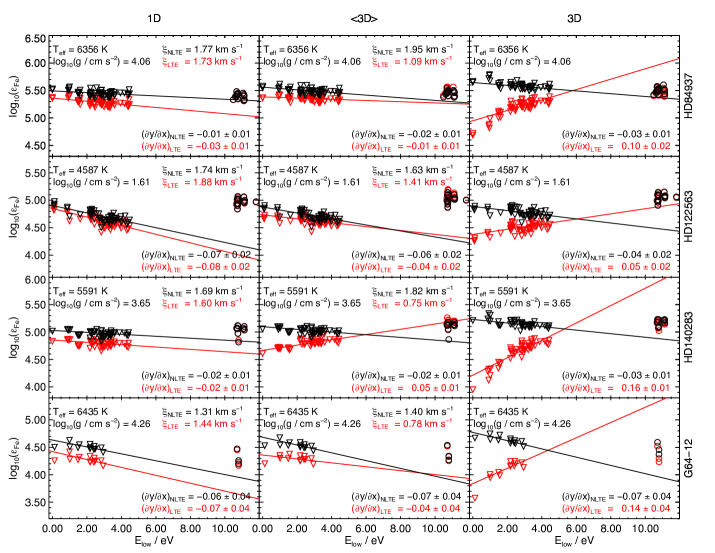
Figure 2: Inferred iron abundance against excitation energy for selected Fe i and Fe ii lines. The excitation energies for both species are given relative to the ground state of Fe i, such that the ground state of Fe ii has $E_{\mathrm{low}}=7.9024\,\mathrm{eV}$. Rows from top to bottom show the different benchmark stars: HD84937, HD122563, HD140283, and G64-12. Columns from left to right show the different paradigms: 1D radiative transfer with theoretical 1D marcs model atmospheres, 1D radiative transfer with ⟨3D⟩ stagger model atmospheres, and full 3D radiative transfer with 3D stagger model atmospheres. Fe i lines are indicated with black triangles (non-LTE) and red triangles (LTE); Fe ii lines are indicated with black circles (non-LTE) and red circles (LTE). The least-squares trend with excitation energy of the Fe i lines is overdrawn; the standard error in the gradient reflects the uncorrelated errors arising from measurement errors in the observed equivalent widths as well as correlated errors arising from errors in the effective temperatures and surface gravities (Sect. 2.5).

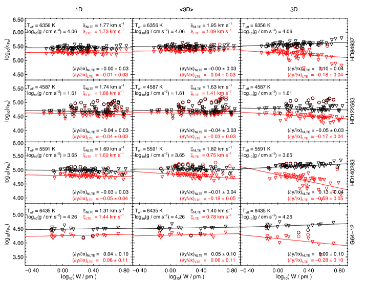
Figure 3: Inferred iron abundance against equivalent width for selected Fe i and Fe ii lines. Rows from top to bottom show the different benchmark stars: HD84937, HD122563, HD140283, and G64-12. Columns from left to right show the different paradigms: 1D radiative transfer with theoretical 1D marcs model atmospheres, 1D radiative transfer with ⟨3D⟩ stagger model atmospheres, and full 3D radiative transfer with 3D stagger model atmospheres. Fe i lines are indicated with black triangles (non-LTE) and red triangles (LTE); Fe ii lines are indicated with black circles (non-LTE) and red circles (LTE). The least-squares trend with (logarithmic) equivalent width of the Fe i lines is overdrawn; the standard error in the gradient reflects the uncorrelated errors arising from measurement errors in the observed equivalent widths as well as correlated errors arising from errors in the effective temperatures and surface gravities (Sect. 2.5). The microturbulent parameter $\xi$ in the 1D and ⟨3D⟩ analyses was calibrated to flatten these trends, without considering the uncertainties in the effective temperatures and surface gravities. If these uncertainties were considered in the calibration of $\xi$, then the trends in the first two columns would be identically zero.

For a given star, individual iron abundances were inferred for each line by fitting the theoretical line strengths to the observed equivalent width. The 1D analyses based on marcs and ⟨3D⟩ model atmospheres contain a free parameter: the microturbulent broadening parameter $\xi$. This was calibrated by removing the trend in the inferred iron abundance from Fe i lines against equivalent width. We emphasize that in 3D non-LTE calculations no microturbulence enters into the calculations (Sect. 2.3.1), which is one of the main advantages of using 3D model atmospheres (e.g. Asplund et al., 2000).

Assuming that the nominal measured effective temperatures and surface gravities of the benchmark stars, and their standard errors, are accurate (Table 1), the reliability of the 3D non-LTE spectral line formation calculations can be assessed and quantified by considering the difference between the iron abundances that are a) inferred from Fe i lines and from Fe ii lines (ionization balance); b) inferred from low-excitation Fe i lines and high-excitation Fe i lines (excitation balance); and c) inferred from weak and strong Fe lines. We illustrate this in Table 3, Fig. 2 and Fig. 3, and discuss different aspects of the results below.

3.1 3D non-LTE Fe line formation

The trends in iron abundance with excitation energy inferred from Fe i lines take the same shape in all cases, having a slight, yet significant, negative gradient. Fig. 2 shows that the mean difference between the iron abundances inferred from the lowest and highest excitation Fe i lines is roughly $0.1\,\mathrm{dex}$ for HD84937 and HD140283, which have the most significant gradients. The corresponding trends in inferred iron abundance with equivalent width are less significant, with the trend for G64-12 being consistent with zero. Fig. 3 shows that, as with the trend with excitation energy, HD140283 has the most significant gradient: the mean difference between the iron abundances inferred from the weakest and strongest Fe i lines is of the order $0.1\,\mathrm{dex}$.

Table 3 shows that for HD84937, HD140283, and G64-12 the average 3D non-LTE iron abundances inferred from Fe i lines are larger than those inferred from Fe ii lines, by $0.07\,\mathrm{dex}$, $0.06\,\mathrm{dex}$, and $0.14\,\mathrm{dex}$ respectively. These discrepancies are consistent with the $1\sigma$ standard errors in the mean for HD84937, HD140283, and G64-12. For HD122563, on the other hand, the Fe i result is smaller than the Fe ii result, by $0.26\,\mathrm{dex}$, a $3\sigma$ discrepancy. This large ionization-balance discrepancy is not unique to this work (e.g.  Bergemann et al., 2012, Sect. 4.5.4). Qualitatively, a similar discrepancy is found by the analyses based on the 1D model atmospheres, which suggests that the problem does not lie with the 3D model atmosphere itself. Rather, there may be something peculiar about some other aspect of the non-LTE calculations in this region of parameter space, such as the background opacities or the collisional rate coefficients, or about the stellar parameters that were adopted for this star. Assuming the latter, we predict that the surface gravity of this star is in fact closer to $1.1\,\mathrm{dex}$. With the upcoming Gaia Data Release 1 (Michalik et al., 2015), the parallax of HD122563 will be improved and thus our prediction tested.

Overall, with the exception of the ionization-balance in the metal-poor red giant HD122563, excitation-balance and ionization-balance are obtained to a satisfactory level, and the trends in inferred abundance with equivalent width are flat. Small modelling errors of the order $0.05\,\mathrm{dex}$ are evident however. That the trend with excitation energy takes the same shape in all four stars, as well as in the 1D results (Sect. 3.2), suggests that the non-LTE effects in the low-excitation Fe i may be slightly overestimated. Slightly weaker non-LTE effects would also improve the ionization balance in these stars (except for HD122563). The use of a collisional efficiency scaling factor $S_{\mathrm{H}}$ would mask these modelling uncertainties, as was possibly the case in our previous 1D work (Bergemann et al., 2012).

It is not obvious what exactly is causing this final shortcoming of a slight trend in iron abundance with excitation potential; we note that in 1D analyses such trends can normally be hidden by tuning the microturbulence parameter while in 3D non-LTE there is no such luxury. The results could be hinting at inadequacies in the adopted formulae for collisional excitation and ionization by electron impact (Sect. 2.2), which are based on general approximations that do not take into account the specific properties of the iron atom, and are a clear weakness of the present modelling. Then, an obvious next step in improving the non-LTE modelling and in trying to resolve this issue would be to calculate Fe+e^- collisional cross-sections using modern atomic structure and close-coupling methods such as R-matrix techniques (e.g. Burke et al., 1971; Burke & Robb, 1976; Berrington et al., 1974, 1978), or B-spline R-matrix techniques (e.g. Zatsarinny, 2006; Zatsarinny & Bartschat, 2013). Such data would at the very least rule out the collisional modelling as the origin of the remaining discrepancies.

3.2 1D versus 3D non-LTE line formation

Table 3 reveals that, in non-LTE, larger iron abundances are inferred from Fe i lines from the 3D model atmospheres than from the ⟨3D⟩ model atmospheres. This can be attributed to the effects of atmospheric inhomogeneities and horizontal radiation transfer (Holzreuter & Solanki, 2013). Non-local radiation streaming in from surrounding regions can strengthen and weaken Fe i lines depending on the sign of the temperature contrast (Holzreuter & Solanki, 2013), in this case with a net line-weakening effect in the spatially-averaged Fe i line profiles. Slightly larger iron abundances are inferred from the ⟨3D⟩ model atmospheres than from the marcs model atmospheres. This can be attributed to the differences in the mean temperature stratification predicted by 3D hydrodynamic models and by 1D hydrostatic models (Bergemann et al., 2012). Steeper temperature gradients in the outer layers of the ⟨3D⟩ model atmospheres lead to a greater amount of non-local radiation and consequently a greater degree of overionizaton of neutral iron, which weakens the Fe i lines (Bergemann et al., 2012).

Table 3 also reveals that, larger iron abundances are inferred from the Fe ii lines from the 3D model atmospheres than from the ⟨3D⟩ model atmospheres, and from Fe ii lines from the ⟨3D⟩ model atmospheres than from the marcs model atmospheres. Since the Fe ii lines form close to LTE (Sect. 4.1), these observations must be attributed to differences in the local conditions in the line-forming regions of the respective model atmospheres: temperature and density inhomogeneities and velocity gradients, as well as differences in the mean temperature stratification. The net line-weakening effects are consistent with what have been found in previous 3D LTE investigations, for example Asplund et al. (1999), Collet et al. (2007), Magic et al. (2013b), and Gallagher et al. (2015).

The microturbulent broadening parameter $\xi$, serves to improve the trends in inferred abundance with equivalent width (Fig. 3), but also with excitation energy (Fig. 2), in the 1D analyses relative to the 3D analyses, this free parameter being fitted to remove the trend in inferred iron abundance from Fe i lines with equivalent width. Since $\xi$ affects strong lines, which tend to be of low-excitation, more than it does weak (and high-excitation) lines, it has a strong influence on these trends. Its impact on the ionization balance is smaller, which is why the ionization balance remains comparable in 1D non-LTE to that in 3D non-LTE (Table 3).

HD122563 is best modelled in 3D, even without any free parameters. Fig. 2 shows that the trend in inferred iron abundance with excitation energy is significantly closer to zero with the 3D non-LTE analysis than with the 1D non-LTE analysis using marcs and ⟨3D⟩ model atmospheres. Table 3 shows that 3D non-LTE analysis results in the smallest discrepancy between the non-LTE iron abundances inferred from Fe i lines and those inferred from Fe ii lines. This suggests that 3D models are necessary for accurate spectroscopic analyses of HD122563, and of similar types of stars; however, the large ionization-balance discrepancy found for this star (Sect. 3.1) prevents a stronger conclusion on this point from being drawn.

3.3 LTE versus non-LTE line formation

Our results strongly favour non-LTE Fe i line formation over LTE line formation. Table 3 shows that the discrepancy between the mean inferred abundances from Fe i and Fe ii lines is several standard errors worse in 3D LTE than in 3D non-LTE. Similarly, Fig. 2 and Fig. 3 show that the trends in inferred iron abundance with excitation energy are typically much steeper in 3D LTE than in 3D non-LTE, by several standard errors. This is not surprising: steep temperature gradients and low temperatures in the line-forming regions of low metallicity 3D models make them prone to large departures from LTE (Asplund et al., 1999; Asplund et al., 2003).

At first glance, the difference between the LTE results and the non-LTE results are less pronounced in the 1D calculations than they are in the 3D calculations, in particular with regards to the trends in inferred iron abundance with excitation energy and equivalent width. This can be attributed to the free parameter $\xi$, which serves to mask some of the short-comings of the assumption of LTE in the 1D and ⟨3D⟩ model atmospheres (Sect. 3.2). Also noteworthy are the hotter mean temperature stratifications in the marcs model atmospheres in the outer layers (compared to the mean temperature stratification of the 3D model atmospheres; Fig. 1). The theoretical low-excitation Fe i lines are weaker in higher temperature conditions in LTE, meaning that a larger iron abundance is required to reproduce the observations. This flattens the trend in inferred iron abundance with excitation energy obtained with the marcs model atmospheres in LTE.

In summary, it is particularly important to carry out non-LTE calculations when using 3D model atmospheres at low metallicity for elements susceptible to non-LTE effects.

3.4 Best inferred iron abundances

Table 4: Best estimate of the iron abundances of the benchmark stars using the best literature values of the effective temperatures and surface gravities (Table 1), and non-LTE results from the 3D stagger model atmospheres. Absolute abundances $\log{\epsilon_{\mathrm{Fe}}}$ were converted to relative abundances $\mathrm{\left[Fe/H\right]}$ by adopting for the solar iron abundance $\log{\epsilon_{\mathrm{Fe\odot}}}=7.47$, which is the value found by Scott et al. (2015) from an analysis based on a 3D stagger model atmospheres and Fe i and Fe ii lines. The stipulated errorsreflect the uncertainties in the equivalent widths, oscillator strengths, effective temperatures and surface gravities (Sect. 2.5). Systematic modelling errors have been estimated by taking half the difference between the abundances inferred from Fe i and Fe ii lines.

Star	$\mathrm{\left[Fe/H\right]}$
HD84937	$-1.96\pm 0.02\text{(stat)}\pm 0.04\text{(sys)}$
HD122563	$-2.49\pm 0.11\text{(stat)}\pm 0.14\text{(sys)}$
HD140283	$-2.31\pm 0.03\text{(stat)}\pm 0.03\text{(sys)}$
G64-12	$-2.94\pm 0.06\text{(stat)}\pm 0.06\text{(sys)}$

We provide our best inferred iron abundances for the four benchmark stars in Table 4. These were computed from the mean of the iron abundances inferred from the Fe i and Fe ii lines using a 3D non-LTE analysis (i.e. by combining the last two columns and last four rows of Table 3), weighted by their standard errors (and without systematic errors included). Although the inferred abundances are consistent with those of Bergemann et al. (2012), listed in Table 1, to within the standard errors, our results are typically higher than their results. This can be attributed to 3D effects (Sect. 4.2) as well as larger non-LTE effects resulting from improved atomic data, especially neutral hydrogen collisional rate coefficients (Sect. 4.3).

4 Grids of non-LTE abundance corrections

Figure 4: Abundance corrections based on equivalent widths. Each panel shows a typical high-excitation Fe i line for different sets of stellar parameters; the plots are truncated after the line becomes saturated in LTE (reduced equivalent widths smaller than -4.9 dex). Several different types of correction are shown: 3D non-LTE versus ⟨3D⟩ non-LTE corrections; ⟨3D⟩ non-LTE versus 1D non-LTE corrections; 1D non-LTE versus 1D LTE corrections from this work; and 1D non-LTE versus 1D LTE abundance corrections, using marcs model atmospheres, from Lind et al. (2012). The L12 results were shifted in $\mathrm{\left[Fe/H\right]}$ to put them on the same absolute scale, where the reference solar iron abundance is $\log{\epsilon_{\mathrm{Fe\odot}}}=7.5$.

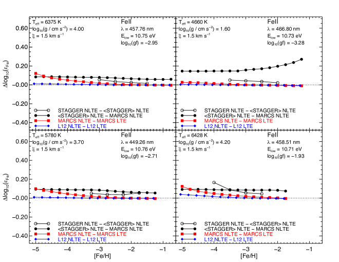
Figure 5: Abundance corrections based on equivalent widths. Each panel shows a typical Fe ii line for different sets of stellar parameters; the plots are truncated after the line becomes saturated in LTE (reduced equivalent widths smaller than -4.9 dex). The excitation energies are given relative to the ground state of Fe i, such that the ground state of Fe ii has $E_{\mathrm{low}}=7.9024\,\mathrm{eV}$. Several different types of correction are shown: 3D non-LTE versus ⟨3D⟩ non-LTE corrections; ⟨3D⟩ non-LTE versus 1D non-LTE corrections; 1D non-LTE versus 1D LTE corrections from this work; and 1D non-LTE versus 1D LTE abundance corrections, using marcs model atmospheres, from Lind et al. (2012). The L12 results were shifted in $\mathrm{\left[Fe/H\right]}$ to put them on the same absolute scale, where the reference solar iron abundance is $\log{\epsilon_{\mathrm{Fe\odot}}}=7.5$.

Grids of equivalent widths and abundance corrections were constructed for 2086 Fe i lines and 115 Fe ii lines for which accurate experimental atomic data exist. These results can be accessed on the INSPECT database, or by contacting the authors. Abundance corrections for other Fe i and Fe ii lines can be obtained by interpolation on the irregular grid of line parameters $\left(\lambda,\mathrm{E}_{\text{low}},\log g\,f\right)$; interpolation routines for that purpose are available upon request.

Grids of departure coefficients are also available, which are more appropriate when higher precision and accuracy is required, and when an analysis based on spectral line profile fitting, rather than on equivalent widths, is called for. The departure coefficients can be used to correct the LTE populations in LTE spectral line synthesis codes, to obtain non-LTE spectral lines and equivalent widths with almost no added computational cost.

We illustrate abundance corrections, based on equivalent widths, for typical Fe i lines (Fig. 4) and Fe ii lines (Fig. 5), and discuss their characteristics below.

4.1 Non-LTE effect

In line with previous non-LTE studies for iron (e.g. Thévenin & Idiart, 1999; Korn et al., 2003; Collet et al., 2005; Mashonkina et al., 2011; Lind et al., 2012; Sitnova et al., 2015), Fig. 4 shows that the Fe i lines are significantly stronger in non-LTE than they are in LTE, at least in the metal-poor regime. The 1D non-LTE versus 1D LTE abundance corrections are positive, and increasing towards lower $\mathrm{\left[Fe/H\right]}$. This is consistent with the overionization picture that we described in Sect. 1. The abundance corrections are in fact typically monotonic with stellar parameters increasing with increasing $T_{\mathrm{eff}}$, decreasing $\log{g}$, and decreasing $\mathrm{\left[Fe/H\right]}$ (Lind et al., 2012, Fig. 2).

The overionization effect on Fe i lines is very weak in the solar-metallicity and metal-rich regimes (Lind et al. in preparation). For some sets of stellar parameters, the 1D non-LTE versus 1D LTE abundance corrections are even slightly negative, reaching $-0.05\,\mathrm{dex}$ at $\mathrm{\left[Fe/H\right]}\approx 0.5$. Overionization is weaker in this regime; photon suction driven by photon losses in the lines becomes relatively important (Bergemann et al., 2012). Since the absolute size of the corrections are so small in this regime, the results are relatively sensitive to the amount of background opacity in the UV, with more background opacity serving to reduce the overionization effect (e.g. Takeda, 1991, Sect. 4.3). We were therefore careful to use recent opacity data for background lines and continua, as we discussed in Sect. 2.1.2.

Fig. 5 shows that the non-LTE effects in Fe ii lines are not strictly non-zero in the metal-poor regime. With marcs models, they are negligible for $\mathrm{\left[Fe/H\right]}\gtrsim-2.5$, but grow with decreasing $\mathrm{\left[Fe/H\right]}$. Since 3D non-LTE abundances are significantly larger than 1D non-LTE abundances (Sect. 3.2), this suggests that the metallicities of the most metal-poor stars (Christlieb et al., 2002; Frebel et al., 2007; Bessell et al., 2015) have hitherto been underestimated (Nordlander et al., 2016). This is true regardless of whether (or which) Fe i or Fe ii lines have been used.

4.2 3D effect

The impact of using 3D radiative transfer and 3D hydrodynamic model atmospheres on the inferred iron abundance can be decoupled into two separate effects: the effect of atmospheric inhomogeneities and horizontal radiation transfer (Holzreuter & Solanki, 2013), and the effect of differences in the mean temperature stratification. In this section we compare the relative sizes of the different effects, having discussed them already in Sect. 3.2. The former type of effects are quantified by the 3D versus ⟨3D⟩ abundance corrections, and the latter type are quantified by the ⟨3D⟩ versus 1D abundance corrections. This decoupling is only to aid one’s intuition: the two effects are not orthogonal, and their relative sizes are sensitive to how the ⟨3D⟩ model atmospheres are constructed.

For Fe i lines the effect of atmospheric inhomogeneities and horizontal radiation transfer is small but significant: Fig. 4 shows that the 3D non-LTE versus ⟨3D⟩ non-LTE abundance corrections are of the order $0.1\,\mathrm{dex}$. This appears to be more severe than the effect of differences in the mean temperature stratification: the magnitudes of the ⟨3D⟩ non-LTE versus 1D non-LTE abundance corrections for Fe i lines are typically smaller than $0.05\,\mathrm{dex}$. For Fe ii lines the two effects tend to be of comparable size ($0.05$-$0.10\,\mathrm{dex}$) and are of the same sign, compounding each other. This means that 3D effects are more pronounced in Fe ii lines than in Fe i lines, amounting to 3D non-LTE abundances that are of the order $0.1\,\mathrm{dex}$ higher than in 1D non-LTE with marcs model atmospheres.

In other words, with 1D marcs model atmospheres and non-LTE radiative transfer, both Fe i and Fe ii lines underestimate the true iron abundance by roughly $0.1\,\mathrm{dex}$ (as judged by the 3D non-LTE analysis; cf. Sect. 3, Table 3). Obviously Fe i lines in LTE suffer from even larger systematic errors at low $\mathrm{\left[Fe/H\right]}$ and thus their use should be avoided.

4.3 Comparison with Lind et al. (2012)

The main differences between the 1D radiative transfer calculations in 1D marcs model atmospheres carried out in this work, and the analogous calculations carried out by Lind et al. (2012), relate to the model atom and in particular to the treatment of the neutral hydrogen collisional rate coefficients. Lind et al. (2012) used semi-empirical hydrogen collisional rate coefficients from Drawin (1968, 1969) with collisional efficiency scaling factor $S_{\mathrm{H}}=1.0$, which was calibrated in Bergemann et al. (2012) so as to obtain ionization balance in benchmark stars. As we discussed in Sect. 1 (see also Barklem et al., 2011; Barklem, 2016a), this empirical approach is based on a classical formula that does not provide a good description of the actual quantum-mechanical physics. In contrast, the model atom employed in this work utilized new quantum-mechanical calculations for the neutral hydrogen collisional rate coefficients, which are expected to be more accurate than the previous classical description by orders of magnitude (Barklem, 2016b).

The 1D non-LTE versus 1D LTE abundance corrections predicted by Lind et al. (2012) for Fe i and Fe ii lines using marcs model atmospheres are typically smaller than the corresponding abundance corrections obtained here by about 0.1 to 0.2 dex; for metal-poor giants the two sets of calculations are more similar. A smaller choice of $S_{\mathrm{H}}$ in their calculations would have increased their non-LTE effects, thereby improving the agreement between their results and our own. It is important to appreciate, however, that calibrating $S_{\mathrm{H}}$ masks inadequacies in the models, that are not limited to the description of the neutral hydrogen collisional rate coefficients themselves.

5 Conclusions

We have presented the first 3D non-LTE line formation calculations for iron with quantum mechanical neutral hydrogen collisional rate coefficients data. The calculations were done for four metal-poor benchmark stars: HD84937, HD122563, HD140283, and G64-12. This type of analysis benefits from the absence of two free parameters: the microturbulent broadening parameter $\xi$, necessary in analyses based on 1D model atmospheres to account for line broadening by convective motions, and the collisional efficiency scaling factor $S_{\mathrm{H}}$, necessary in analyses based on the classical semi-empirical recipe of Drawin (1968, 1969) for the neutral hydrogen collisional rate coefficients.

Our main conclusions are:

• With the exception of the metal-poor red giant HD122563, the 3D non-LTE spectral line formation calculations appear to be accurate to about $\pm 0.05\,\mathrm{dex}$ in inferred iron abundance. Systematic modelling errors of this order are possibly due to the non-LTE effects being overestimated, which has hitherto gone unnoticed because they were hidden in the calibration of the free parameter $S_{\mathrm{H}}$. Modern quantum-mechanical electron collision cross-sections for iron are needed to place the collisional modelling on a firm footing. It is extremely important that such calculations be done and we advocate that this should be investigated as the possible source of remaining discrepancies before considering more exotic explanations.

• We predict that the parallax-based surface gravity of HD122563 is overestimated, on the basis that, in contrast to the other three stars, much larger non-LTE effects than what we currently predict would be required to rectify the observed ionization-imbalance. We predict $\log{g}\approx 1.1$ for this star.

• The new quantum-mechanical neutral hydrogen collisional rate coefficients result in larger non-LTE effects than do the recipe of Drawin (1968, 1969) with $S_{\mathrm{H}}=1.0$.

• 3D effects in Fe i lines caused by atmospheric inhomogeneities and horizontal radiation transfer are typically more severe than those caused by differences in the mean temperature stratifications; the two effects in Fe ii lines are typically of comparable size and have the same sign. Overall, the 3D effects go in the same direction as the non-LTE effects, requiring positive abundance corrections. Fe ii lines are slightly more prone to these effects than Fe i lines.

• As a consequence of the 3D effects and larger non-LTE effects, our inferred iron abundances for the four benchmark stars are slightly higher than in our previous 1D non-LTE study (Bergemann et al., 2012).

Extended grids of abundance corrections and equivalent widths based on full 3D non-LTE calculations are still somewhat beyond reach with today’s computational resources. Nevertheless, we have made available grids of departure coefficients and abundance corrections based on 1D marcs model atmospheres and ⟨3D⟩ model atmospheres (Sect. 4). A future work may consider the construction of 3D LTE grids of abundance corrections for Fe ii lines; such grids would be valid in the regime $\mathrm{\left[Fe/H\right]}\gtrsim-2.5$. We recommend that such grids be implemented into future spectroscopic stellar analyses that are based on Fe i and Fe ii lines, including large-scale surveys such as APOGEE (Majewski et al., 2015), GALAH (De Silva et al., 2015), 4MOST (de Jong et al., 2014), and WEAVE (Dalton et al., 2014).

Appendix A Line lists

Table 5: Fe ilines analysed in the various benchmark stars.

$\lambda_{\mathrm{Air}}/\mathrm{nm}$	Lower level	Upper level	$J_{\mathrm{low}}$	$J_{\mathrm{up}}$	$E_{\mathrm{low}}/\mathrm{eV}$	$\log{g\,f}$	$\text{Equivalent width}/\text{pm}$
							HD84937	HD122563	HD140283	G64-12
344.52	3d7.(4P).4s a$\,{}^{5}$P	3d7.(4P).4p u$\,{}^{5}$D	2.0	3.0	2.1979	-0.535g				0.79
347.67	3d6.(5D).4s2 a$\,{}^{5}$D	3d6.(5D).4s.4p z$\,{}^{5}$P	0.0	1.0	0.1213	-1.506g				3.62
386.55	3d7.(4F).4s a$\,{}^{5}$F	3d7.(4F).4p y$\,{}^{5}$D	1.0	1.0	1.0111	-0.950g				3.41
395.00	3d7.(4P).4s a$\,{}^{5}$P	3d6.(3P).4s.4p x$\,{}^{5}$P	3.0	2.0	2.1759	-1.251g	2.17
400.17	3d7.(4P).4s a$\,{}^{5}$P	3d6.(3P).4s.4p x$\,{}^{5}$P	3.0	3.0	2.1759	-1.901g			0.93
400.73	3d7.(2G).4s a$\,{}^{3}$G	3d6.(3F).4s.4p x$\,{}^{3}$F	3.0	2.0	2.7586	-1.276g	0.77		0.78
400.97	3d7.(4P).4s a$\,{}^{5}$P	3d6.(3P).4s.4p x$\,{}^{5}$P	1.0	2.0	2.2227	-1.252g	2.23		2.68
402.19	3d7.(2G).4s a$\,{}^{3}$G	3d6.(3H).4s.4p z$\,{}^{3}$H	3.0	4.0	2.7586	-0.729g	2.35
404.46	3d7.(4P).4s b$\,{}^{3}$P	3d7.(4P).4p y$\,{}^{3}$S	2.0	1.0	2.8316	-1.221g	0.92		1.06
406.24	3d7.(4P).4s b$\,{}^{3}$P	3d7.(4P).4p y$\,{}^{3}$S	1.0	1.0	2.8450	-0.862g	1.59		1.74
413.99	3d7.(4F).4s a$\,{}^{5}$F	3d6.(5D).4s.4p z$\,{}^{3}$F	2.0	2.0	0.9901	-3.514g		3.64
414.77	3d7.(4F).4s a$\,{}^{3}$F	3d7.(4F).4p z$\,{}^{3}$G	4.0	3.0	1.4849	-2.071g	1.74
415.88	3d6.(5D).4s.4p z$\,{}^{5}$F	3d6.(5D).4s.4d f$\,{}^{5}$F	1.0	2.0	3.4302	-0.700h	0.86
418.49	3d7.(4P).4s b$\,{}^{3}$P	3d6.(3P).4s.4p y$\,{}^{3}$P	2.0	2.0	2.8316	-0.869g	1.61		1.81
419.62	3d6.(5D).4s.4p z$\,{}^{5}$F	3d6.(5D).4s.4d e$\,{}^{5}$G	3.0	3.0	3.3965	-0.696g	0.86		0.94
420.20	3d7.(4F).4s a$\,{}^{3}$F	3d7.(4F).4p z$\,{}^{3}$G	4.0	4.0	1.4849	-0.689g				2.82
421.62	3d6.(5D).4s2 a$\,{}^{5}$D	3d6.(5D).4s.4p z$\,{}^{7}$P	4.0	4.0	0.0000	-3.357g	2.16		3.69
421.94	3d7.(2H).4s a$\,{}^{1}$H	3d7.(2H).4p y3I	5.0	6.0	3.5732	0.000g	2.56		2.48
422.22	3d6.(5D).4s.4p z$\,{}^{7}$D	3d6.(5D).4s.5s e$\,{}^{7}$D	3.0	3.0	2.4496	-0.914g	2.61		2.99
423.59	3d6.(5D).4s.4p z$\,{}^{7}$D	3d6.(5D).4s.5s e$\,{}^{7}$D	4.0	4.0	2.4254	-0.340i				1.27
423.88	3d6.(5D).4s.4p z$\,{}^{5}$F	3d6.(5D).4s.4d e$\,{}^{5}$G	3.0	4.0	3.3965	-0.233g	2.14		2.15
425.01	3d6.(5D).4s.4p z$\,{}^{7}$D	3d6.(5D).4s.5s e$\,{}^{7}$D	2.0	3.0	2.4688	-0.380g	4.97			0.98
426.05	3d6.(5D).4s.4p z$\,{}^{7}$D	3d6.(5D).4s.5s e$\,{}^{7}$D	5.0	5.0	2.3992	0.077g				2.49
428.24	3d7.(4P).4s a$\,{}^{5}$P	3d6.(3P).4s.4p z$\,{}^{5}$S	3.0	2.0	2.1759	-0.779g	4.27		4.81	0.71
437.59	3d6.(5D).4s2 a$\,{}^{5}$D	3d6.(5D).4s.4p z$\,{}^{7}$F	4.0	5.0	0.0000	-3.005g	3.72
440.48	3d7.(4F).4s a$\,{}^{3}$F	3d7.(4F).4p z$\,{}^{5}$G	3.0	4.0	1.5574	-0.147g				5.26
440.84	3d7.(4P).4s a$\,{}^{5}$P	3d6.(5D).4s.4p x$\,{}^{5}$D	2.0	1.0	2.1979	-1.775g	1.07
442.26	3d7.(4P).4s b$\,{}^{3}$P	3d6.(3P).4s.4p x$\,{}^{3}$D	1.0	1.0	2.8450	-1.115g	1.14		1.25
445.44	3d7.(4P).4s b$\,{}^{3}$P	3d6.(3P).4s.4p x$\,{}^{3}$D	2.0	2.0	2.8316	-1.298g	0.73
446.66	3d7.(4P).4s b$\,{}^{3}$P	3d6.(3P).4s.4p x$\,{}^{3}$D	2.0	3.0	2.8316	-0.600g	2.64
448.42	3d6.(5D).4s.4p z$\,{}^{5}$P	3d6.(5D).4s.5s g$\,{}^{5}$D	3.0	4.0	3.6025	-0.640h	0.61	1.83
449.46	3d7.(4P).4s a$\,{}^{5}$P	3d6.(5D).4s.4p x$\,{}^{5}$D	2.0	3.0	2.1979	-1.143g	2.86		3.63
452.86	3d7.(4P).4s a$\,{}^{5}$P	3d6.(5D).4s.4p x$\,{}^{5}$D	3.0	4.0	2.1759	-0.887g				0.72
453.12	3d7.(4F).4s a$\,{}^{3}$F	3d7.(4F).4p y$\,{}^{5}$F	4.0	4.0	1.4849	-2.101g	1.71		2.33
454.79	3d7.(a$\,{}^{2}$D).4s a$\,{}^{1}$D	3d7.(2G).4p z$\,{}^{1}$F	2.0	3.0	3.5465	-1.012g		1.40
461.93	3d6.(5D).4s.4p z$\,{}^{5}$P	3d6.(5D).4s.4d f$\,{}^{5}$D	3.0	2.0	3.6025	-1.060h		0.91
463.01	3d6.(3P).4s2 a$\,{}^{3}$P	3d6.(5D).4s.4p x$\,{}^{5}$D	2.0	3.0	2.2786	-2.587g		1.50
467.89	3d6.(5D).4s.4p z$\,{}^{5}$P	3d6.(5D).4s.4d f$\,{}^{5}$D	3.0	4.0	3.6025	-0.680h		1.95
473.68	3d6.(5D).4s.4p z$\,{}^{5}$D	3d7.(4F).5s e$\,{}^{5}$F	4.0	5.0	3.2112	-0.670h	1.31		1.44
474.15	3d7.(4P).4s b$\,{}^{3}$P	3d6.(3P).4s.4p w$\,{}^{5}$D	2.0	3.0	2.8316	-1.764g		1.07
478.88	3d7.(2H).4s b$\,{}^{3}$H	3d6.(3H).4s.4p z$\,{}^{3}$H	6.0	6.0	3.2367	-1.763g		0.57
488.21	3d6.(5D).4s.4p z$\,{}^{5}$F	3d7.(4F).5s e$\,{}^{5}$F	2.0	2.0	3.4170	-1.480h		0.72
491.90	3d6.(5D).4s.4p z$\,{}^{7}$F	3d6.(5D).4s.5s e$\,{}^{7}$D	3.0	3.0	2.8654	-0.342g	3.74		3.99
492.05	3d6.(5D).4s.4p z$\,{}^{7}$F	3d6.(5D).4s.5s e$\,{}^{7}$D	5.0	4.0	2.8325	0.070i			6.14	1.38
493.88	3d6.(5D).4s.4p z$\,{}^{7}$F	3d6.(5D).4s.5s e$\,{}^{7}$D	2.0	3.0	2.8755	-1.077g	1.02	4.29
494.64	3d6.(5D).4s.4p z$\,{}^{5}$F	3d7.(4F).5s e$\,{}^{5}$F	4.0	4.0	3.3683	-1.110i		1.75
495.01	3d6.(5D).4s.4p z$\,{}^{5}$F	3d7.(4F).5s e$\,{}^{5}$F	2.0	3.0	3.4170	-1.500h		0.67
496.61	3d6.(5D).4s.4p z$\,{}^{5}$F	3d7.(4F).5s e$\,{}^{5}$F	5.0	5.0	3.3320	-0.790h	0.88
497.31	3d6.(5D).4s.4p z$\,{}^{3}$D	3d6.(5D).4s.5s e$\,{}^{3}$D	1.0	1.0	3.9597	-0.690i		0.90
500.19	3d6.(5D).4s.4p z$\,{}^{3}$F	3d6.(5D).4s.5s e$\,{}^{3}$D	4.0	3.0	3.8816	-0.010i			1.38
500.61	3d6.(5D).4s.4p z$\,{}^{7}$F	3d6.(5D).4s.5s e$\,{}^{7}$D	5.0	5.0	2.8325	-0.615g	2.60		2.89
501.21	3d7.(4F).4s a$\,{}^{5}$F	3d6.(5D).4s.4p z$\,{}^{5}$F	5.0	5.0	0.8590	-2.642b			3.36
501.49	3d6.(5D).4s.4p z$\,{}^{3}$F	3d6.(5D).4s.5s e$\,{}^{3}$D	3.0	2.0	3.9433	-0.180h	0.96	2.27
502.22	3d6.(5D).4s.4p z$\,{}^{3}$F	3d6.(5D).4s.5s e$\,{}^{3}$D	2.0	1.0	3.9841	-0.330i		1.40
504.98	3d6.(3P).4s2 a$\,{}^{3}$P	3d7.(4F).4p y$\,{}^{3}$D	2.0	3.0	2.2786	-1.355g	1.80		2.25
505.16	3d7.(4F).4s a$\,{}^{5}$F	3d6.(5D).4s.4p z$\,{}^{5}$F	4.0	4.0	0.9146	-2.795b			2.39
506.88	3d6.(5D).4s.4p z$\,{}^{7}$P	3d6.(5D).4s.5s e$\,{}^{7}$D	4.0	3.0	2.9398	-1.041g	1.06	4.07
513.37	3d7.(4F).4p y$\,{}^{5}$F	3d7.(4F).4d f$\,{}^{5}$G	5.0	6.0	4.1777	0.360h	1.84		1.59

Table 6: continued

Fe ilines analysed in the various benchmark stars. $\lambda_{\mathrm{Air}}/\mathrm{nm}$ Lower level Upper level $J_{\mathrm{low}}$ $J_{\mathrm{up}}$ $E_{\mathrm{low}}/\mathrm{eV}$ $\log{g\,f}$ $\text{Equivalent width}/\text{pm}$ HD84937 HD122563 HD140283 G64-12 517.16 3d⁷.(⁴F).4s a$\,{}^{3}$F 3d⁶.(⁵D).4s.4p z$\,{}^{3}$F 4.0 4.0 1.4849 -1.721^g 3.35 4.28 519.14 3d⁶.(⁵D).4s.4p z$\,{}^{7}$P 3d⁶.(⁵D).4s.5s e$\,{}^{7}$D 2.0 1.0 3.0385 -0.551^g 6.09 2.28 519.23 3d⁶.(⁵D).4s.4p z$\,{}^{7}$P 3d⁶.(⁵D).4s.5s e$\,{}^{7}$D 3.0 3.0 2.9980 -0.421^g 2.65 3.02 519.49 3d⁷.(⁴F).4s a$\,{}^{3}$F 3d⁶.(⁵D).4s.4p z$\,{}^{3}$F 3.0 3.0 1.5574 -2.021^g 1.84 2.47 519.87 3d⁷.(⁴P).4s a$\,{}^{5}$P 3d⁶.(⁵D).4s.4p y$\,{}^{5}$P 1.0 2.0 2.2227 -2.135^c 3.87 521.52 3d⁶.(⁵D).4s.4p z$\,{}^{5}$D 3d⁶.(⁵D).4s.5s e$\,{}^{5}$D 2.0 1.0 3.2657 -0.860^h 2.81 521.63 3d⁷.(⁴F).4s a$\,{}^{3}$F 3d⁶.(⁵D).4s.4p z$\,{}^{3}$F 2.0 2.0 1.6079 -2.082^g 1.37 2.10 522.55 3d⁶.(⁵D).4s² a$\,{}^{5}$D 3d⁶.(⁵D).4s.4p z$\,{}^{7}$D 1.0 1.0 0.1101 -4.789^a 4.78 523.29 3d⁶.(⁵D).4s.4p z$\,{}^{7}$P 3d⁶.(⁵D).4s.5s e$\,{}^{7}$D 4.0 5.0 2.9398 -0.057^g 0.75 524.71 3d⁶.(⁵D).4s² a$\,{}^{5}$D 3d⁶.(⁵D).4s.4p z$\,{}^{7}$D 2.0 3.0 0.0873 -4.946^a 3.91 525.50 3d⁶.(⁵D).4s² a$\,{}^{5}$D 3d⁶.(⁵D).4s.4p z$\,{}^{7}$D 1.0 2.0 0.1101 -4.764^a 5.28 526.33 3d⁶.(⁵D).4s.4p z$\,{}^{5}$D 3d⁶.(⁵D).4s.5s e$\,{}^{5}$D 2.0 2.0 3.2657 -0.870^h 0.74 2.94 528.18 3d⁶.(⁵D).4s.4p z$\,{}^{7}$P 3d⁶.(⁵D).4s.5s e$\,{}^{7}$D 2.0 3.0 3.0385 -0.833^g 1.27 4.63 1.48 528.36 3d⁶.(⁵D).4s.4p z$\,{}^{5}$D 3d⁶.(⁵D).4s.5s e$\,{}^{5}$D 3.0 3.0 3.2410 -0.450^h 2.06 530.23 3d⁶.(⁵D).4s.4p z$\,{}^{5}$D 3d⁶.(⁵D).4s.5s e$\,{}^{5}$D 1.0 2.0 3.2830 -0.730^h 3.65 1.10 530.74 3d⁷.(⁴F).4s a$\,{}^{3}$F 3d⁶.(⁵D).4s.4p z$\,{}^{3}$F 2.0 3.0 1.6079 -2.912^g 3.59 532.42 3d⁶.(⁵D).4s.4p z$\,{}^{5}$D 3d⁶.(⁵D).4s.5s e$\,{}^{5}$D 4.0 4.0 3.2112 -0.110ⁱ 3.24 3.47 533.99 3d⁶.(⁵D).4s.4p z$\,{}^{5}$D 3d⁶.(⁵D).4s.5s e$\,{}^{5}$D 2.0 3.0 3.2657 -0.630^h 1.17 4.19 1.34 534.10 3d⁷.(⁴F).4s a$\,{}^{3}$F 3d⁶.(⁵D).4s.4p z$\,{}^{3}$D 2.0 2.0 1.6079 -1.953^g 2.15 536.49 3d⁷.(⁴F).4p z$\,{}^{5}$G 3d⁷.(⁴F).4d e$\,{}^{5}$H 2.0 3.0 4.4456 0.228^g 1.04 536.75 3d⁷.(⁴F).4p z$\,{}^{5}$G 3d⁷.(⁴F).4d e$\,{}^{5}$H 3.0 4.0 4.4153 0.443^g 1.33 1.23 537.00 3d⁷.(⁴F).4p z$\,{}^{5}$G 3d⁷.(⁴F).4d e$\,{}^{5}$H 4.0 5.0 4.3714 0.536^g 1.78 2.97 537.15 3d⁷.(⁴F).4s a$\,{}^{5}$F 3d⁶.(⁵D).4s.4p z$\,{}^{5}$D 3.0 2.0 0.9582 -1.645^b 6.71 538.34 3d⁷.(⁴F).4p z$\,{}^{5}$G 3d⁷.(⁴F).4d e$\,{}^{5}$H 5.0 6.0 4.3125 0.645^g 3.73 1.97 539.32 3d⁶.(⁵D).4s.4p z$\,{}^{5}$D 3d⁶.(⁵D).4s.5s e$\,{}^{5}$D 3.0 4.0 3.2410 -0.720ⁱ 1.23 539.71 3d⁷.(⁴F).4s a$\,{}^{5}$F 3d⁶.(⁵D).4s.4p z$\,{}^{5}$D 4.0 4.0 0.9146 -1.993^b 5.02 6.58 541.09 3d⁷.(⁴F).4p z$\,{}^{3}$G 3d⁷.(⁴F).4d e$\,{}^{3}$H 3.0 4.0 4.4733 0.398^g 1.17 2.05 541.52 3d⁷.(⁴F).4p z$\,{}^{3}$G 3d⁷.(⁴F).4d e$\,{}^{3}$H 5.0 6.0 4.3865 0.643^g 2.01 3.37 1.66 542.97 3d⁷.(⁴F).4s a$\,{}^{5}$F 3d⁶.(⁵D).4s.4p z$\,{}^{5}$D 3.0 3.0 0.9582 -1.879^b 5.62 543.45 3d⁷.(⁴F).4s a$\,{}^{5}$F 3d⁶.(⁵D).4s.4p z$\,{}^{5}$D 1.0 0.0 1.0111 -2.122^b 5.37 544.69 3d⁷.(⁴F).4s a$\,{}^{5}$F 3d⁶.(⁵D).4s.4p z$\,{}^{5}$D 2.0 2.0 0.9901 -1.914^g 1.05 549.75 3d⁷.(⁴F).4s a$\,{}^{5}$F 3d⁶.(⁵D).4s.4p z$\,{}^{5}$D 1.0 2.0 1.0111 -2.849^b 1.93 550.68 3d⁷.(⁴F).4s a$\,{}^{5}$F 3d⁶.(⁵D).4s.4p z$\,{}^{5}$D 2.0 3.0 0.9901 -2.797^b 1.43 556.96 3d⁶.(⁵D).4s.4p z$\,{}^{5}$F 3d⁶.(⁵D).4s.5s e$\,{}^{5}$D 2.0 1.0 3.4170 -0.520^h 1.25 3.82 1.29 557.28 3d⁶.(⁵D).4s.4p z$\,{}^{5}$F 3d⁶.(⁵D).4s.5s e$\,{}^{5}$D 3.0 2.0 3.3965 -0.280^h 2.09 1.99 558.68 3d⁶.(⁵D).4s.4p z$\,{}^{5}$F 3d⁶.(⁵D).4s.5s e$\,{}^{5}$D 4.0 3.0 3.3683 -0.110^h 2.65 6.31 2.84 561.56 3d⁶.(⁵D).4s.4p z$\,{}^{5}$F 3d⁶.(⁵D).4s.5s e$\,{}^{5}$D 5.0 4.0 3.3320 0.040ⁱ 3.38 562.45 3d⁶.(⁵D).4s.4p z$\,{}^{5}$F 3d⁶.(⁵D).4s.5s e$\,{}^{5}$D 2.0 2.0 3.4170 -0.760^h 2.73 576.30 3d⁶.(⁵D).4s.4p z$\,{}^{3}$P 3d⁶.(⁵D).4s.5s e$\,{}^{3}$D 2.0 3.0 4.2089 -0.360ⁱ 1.03 595.67 3d⁷.(⁴F).4s a$\,{}^{5}$F 3d⁶.(⁵D).4s.4p z$\,{}^{7}$P 5.0 4.0 0.8590 -4.608^e 1.27 619.16 3d⁶.(³H).4s² a$\,{}^{3}$H 3d⁷.(⁴F).4p z$\,{}^{3}$G 5.0 4.0 2.4327 -1.416^g 1.33 1.80 621.34 3d⁷.(⁴P).4s a$\,{}^{5}$P 3d⁷.(⁴F).4p y$\,{}^{5}$D 1.0 1.0 2.2227 -2.481^g 2.20 621.93 3d⁷.(⁴P).4s a$\,{}^{5}$P 3d⁷.(⁴F).4p y$\,{}^{5}$D 2.0 2.0 2.1979 -2.433^c 2.76 623.07 3d⁶.(³F).4s² b$\,{}^{3}$F 3d⁷.(⁴F).4p y$\,{}^{3}$F 4.0 4.0 2.5592 -1.281^d 1.70 6.89 1.97 625.43 3d⁶.(³P).4s² a$\,{}^{3}$P 3d⁶.(⁵D).4s.4p z$\,{}^{3}$P 2.0 1.0 2.2786 -2.443^f 2.62 626.51 3d⁷.(⁴P).4s a$\,{}^{5}$P 3d⁷.(⁴F).4p y$\,{}^{5}$D 3.0 3.0 2.1759 -2.550^c 2.60 629.78 3d⁷.(⁴P).4s a$\,{}^{5}$P 3d⁷.(⁴F).4p y$\,{}^{5}$D 1.0 2.0 2.2227 -2.740^c 1.49 633.53 3d⁷.(⁴P).4s a$\,{}^{5}$P 3d⁷.(⁴F).4p y$\,{}^{5}$D 2.0 3.0 2.1979 -2.177^g 4.02 633.68 3d⁶.(⁵D).4s.4p z$\,{}^{5}$P 3d⁶.(⁵D).4s.5s e$\,{}^{5}$D 1.0 1.0 3.6864 -0.850^h 1.32 635.87 3d⁷.(⁴F).4s a$\,{}^{5}$F 3d⁶.(⁵D).4s.4p z$\,{}^{7}$F 5.0 6.0 0.8590 -4.468^b 1.94 639.36 3d⁶.(³H).4s² a$\,{}^{3}$H 3d⁷.(⁴F).4p z$\,{}^{5}$G 5.0 4.0 2.4327 -1.432^f 6.24 640.00 3d⁶.(⁵D).4s.4p z$\,{}^{5}$P 3d⁶.(⁵D).4s.5s e$\,{}^{5}$D 3.0 4.0 3.6025 -0.270ⁱ 1.51 1.58 641.16 3d⁶.(⁵D).4s.4p z$\,{}^{5}$P 3d⁶.(⁵D).4s.5s e$\,{}^{5}$D 2.0 3.0 3.6537 -0.590^h 2.46 642.14 3d⁶.(³P).4s² a$\,{}^{3}$P 3d⁶.(⁵D).4s.4p z$\,{}^{3}$P 2.0 2.0 2.2786 -2.027^c 4.76 643.08 3d⁷.(⁴P).4s a$\,{}^{5}$P 3d⁷.(⁴F).4p y$\,{}^{5}$D 3.0 4.0 2.1759 -2.006^c 5.78 649.50 3d⁶.(³H).4s² a$\,{}^{3}$H 3d⁷.(⁴F).4p z$\,{}^{5}$G 6.0 5.0 2.4041 -1.273^c 2.53 654.62 3d⁷.(²G).4s a$\,{}^{3}$G 3d⁷.(⁴F).4p y$\,{}^{3}$F 3.0 2.0 2.7586 -1.536^g 3.34 659.29 3d⁷.(²G).4s a$\,{}^{3}$G 3d⁷.(⁴F).4p y$\,{}^{3}$F 4.0 3.0 2.7275 -1.473^g 3.84

Table 7: continued

Fe ilines analysed in the various benchmark stars. $\lambda_{\mathrm{Air}}/\mathrm{nm}$ Lower level Upper level $J_{\mathrm{low}}$ $J_{\mathrm{up}}$ $E_{\mathrm{low}}/\mathrm{eV}$ $\log{g\,f}$ $\text{Equivalent width}/\text{pm}$ HD84937 HD122563 HD140283 G64-12 667.80 3d⁷.(²G).4s a$\,{}^{3}$G 3d⁷.(⁴F).4p y$\,{}^{3}$F 5.0 4.0 2.6924 -1.418^g 5.10 675.01 3d⁶.(³P).4s² a$\,{}^{3}$P 3d⁶.(⁵D).4s.4p z$\,{}^{3}$P 1.0 1.0 2.4242 -2.621^c 1.34

a: Blackwell et al. (1979a); b: Blackwell et al. (1979b); c: Blackwell et al. (1982a); d: Blackwell et al. (1982b); e: Blackwell et al. (1986); f: Bard et al. (1991); g: O’Brian et al. (1991); h: Den Hartog et al. (2014); i: Ruffoni et al. (2014).

Table 8: Fe iilines analysed in the various benchmark stars. The excitation energies are given relative to the ground state of Fe i,such that the ground state of Fe ii has $E_{\mathrm{low}}=7.9024\,\mathrm{eV}$.

$\lambda_{\mathrm{Air}}/\mathrm{nm}$	Lower level	Upper level	$J_{\mathrm{low}}$	$J_{\mathrm{up}}$	$E_{\mathrm{low}}/\mathrm{eV}$	$\log{g\,f}$	$\text{Equivalent width}/\text{pm}$
							HD84937	HD122563	HD140283	G64-12
417.89	3d6.(3P).4s b$\,{}^{4}$P	3d6.(5D).4p z$\,{}^{4}$F	2.5	3.5	10.4850	-2.510a	2.10
430.32	3d6.(3P).4s b$\,{}^{4}$P	3d6.(5D).4p z$\,{}^{4}$D	1.5	1.5	10.6067	-2.560a	1.77
438.54	3d6.(3P).4s b$\,{}^{4}$P	3d6.(5D).4p z$\,{}^{4}$D	0.5	0.5	10.6808	-2.660a	1.59
441.68	3d6.(3P).4s b$\,{}^{4}$P	3d6.(5D).4p z$\,{}^{4}$D	0.5	1.5	10.6808	-2.650a	1.35	4.24	1.21
449.14	3d6.(3F).4s b$\,{}^{4}$F	3d6.(5D).4p z$\,{}^{4}$F	1.5	1.5	10.7579	-2.710a	0.95	3.43	0.75
450.83	3d6.(3F).4s b$\,{}^{4}$F	3d6.(5D).4p z$\,{}^{4}$D	1.5	0.5	10.7579	-2.440a	1.92	5.30	1.70
451.53	3d6.(3F).4s b$\,{}^{4}$F	3d6.(5D).4p z$\,{}^{4}$F	2.5	2.5	10.7465	-2.600a	1.49	4.69	1.29
452.02	3d6.(3F).4s b$\,{}^{4}$F	3d6.(5D).4p z$\,{}^{4}$F	4.5	3.5	10.7090	-2.650a	1.40	4.47	1.16
454.15	3d6.(3F).4s b$\,{}^{4}$F	3d6.(5D).4p z$\,{}^{4}$D	1.5	1.5	10.7579	-2.980a		2.50
457.63	3d6.(3F).4s b$\,{}^{4}$F	3d6.(5D).4p z$\,{}^{4}$D	2.5	2.5	10.7465	-2.950a	0.70	2.38
458.38	3d6.(3F).4s b$\,{}^{4}$F	3d6.(5D).4p z$\,{}^{4}$D	4.5	3.5	10.7090	-1.930a	4.39		3.87	0.71
462.05	3d6.(3F).4s b$\,{}^{4}$F	3d6.(5D).4p z$\,{}^{4}$D	3.5	3.5	10.7305	-3.210a		1.31
466.68	3d6.(3F).4s b$\,{}^{4}$F	3d6.(5D).4p z$\,{}^{4}$F	3.5	4.5	10.7305	-3.280a		1.28
492.39	3d5.(6S).4s2 a$\,{}^{6}$S	3d6.(5D).4p z$\,{}^{6}$P	2.5	1.5	10.7934	-1.260a			5.92
501.84	3d5.(6S).4s2 a$\,{}^{6}$S	3d6.(5D).4p z$\,{}^{6}$P	2.5	2.5	10.7934	-1.100a				1.86
516.90	3d5.(6S).4s2 a$\,{}^{6}$S	3d6.(5D).4p z$\,{}^{6}$P	2.5	3.5	10.7934	-1.000a				2.46
519.76	3d6.(3G).4s a$\,{}^{4}$G	3d6.(5D).4p z$\,{}^{4}$F	2.5	1.5	11.1328	-2.220a	1.34	3.92	1.16
523.46	3d6.(3G).4s a$\,{}^{4}$G	3d6.(5D).4p z$\,{}^{4}$F	3.5	2.5	11.1237	-2.180a	1.68	4.30	1.45
527.60	3d6.(3G).4s a$\,{}^{4}$G	3d6.(5D).4p z$\,{}^{4}$F	4.5	3.5	11.1018	-2.010a	2.03		1.94
531.66	3d6.(3G).4s a$\,{}^{4}$G	3d6.(5D).4p z$\,{}^{4}$F	5.5	4.5	11.0551	-1.870a	3.43		2.65
536.29	3d6.(3G).4s a$\,{}^{4}$G	3d6.(5D).4p z$\,{}^{4}$D	4.5	3.5	11.1018	-2.570a	0.86	2.83
553.48	3d6.(3H).4s b$\,{}^{2}$H	3d6.(5D).4p z$\,{}^{4}$F	5.5	4.5	11.1471	-2.750a		1.73
645.64	3d6.(3D).4s b$\,{}^{4}$D	3d6.(5D).4p z$\,{}^{4}$P	3.5	2.5	11.8058	-2.050a		1.45

a: Meléndez & Barbuy (2009).

We list the lines used for the abundance analyses of the benchmark stars in Table 5 and Table 8.

References

- Akerman et al. (2004) Akerman C. J., Carigi L., Nissen P. E., Pettini M., Asplund M., 2004, A&A, 414, 931
- Amarsi et al. (2015) Amarsi A. M., Asplund M., Collet R., Leenaarts J., 2015, MNRAS, 454, L11
- Amarsi et al. (2016) Amarsi A. M., Asplund M., Collet R., Leenaarts J., 2016, MNRAS, 455, 3735
- Anstee & O’Mara (1995) Anstee S. D., O’Mara B. J., 1995, MNRAS, 276, 859
- Asplund (2005) Asplund M., 2005, ARA&A, 43, 481
- Asplund et al. (1999) Asplund M., Nordlund Å., Trampedach R., Stein R. F., 1999, A&A, 346, L17
- Asplund et al. (2000) Asplund M., Nordlund Å., Trampedach R., Allende Prieto C., Stein R. F., 2000, A&A, 359, 729
- Asplund et al. (2003) Asplund M., Carlsson M., Botnen A. V., 2003, A&A, 399, L31
- Athay & Lites (1972) Athay R. G., Lites B. W., 1972, ApJ, 176, 809
- Bagnulo et al. (2003) Bagnulo S., Jehin E., Ledoux C., Cabanac R., Melo C., Gilmozzi R., ESO Paranal Science Operations Team 2003, The Messenger, 114, 10
- Bailey et al. (2015) Bailey J. E., et al., 2015, Nature, 517, 56
- Bard et al. (1991) Bard A., Kock A., Kock M., 1991, A&A, 248, 315
- Barklem (2016a) Barklem P. S., 2016a, A&A Rev., 24, 9
- Barklem (2016b) Barklem P. S., 2016b, Phys. Rev. A, 93, 042705
- Barklem & Aspelund-Johansson (2005) Barklem P. S., Aspelund-Johansson J., 2005, A&A, 435, 373
- Barklem & Collet (2016) Barklem P. S., Collet R., 2016, A&A, 588, A96
- Barklem & O’Mara (1997) Barklem P. S., O’Mara B. J., 1997, MNRAS, 290, 102
- Barklem et al. (1998a) Barklem P. S., Anstee S. D., O’Mara B. J., 1998a, Publications of the Astron. Soc. of Australia, 15, 336
- Barklem et al. (1998b) Barklem P. S., O’Mara B. J., Ross J. E., 1998b, MNRAS, 296, 1057
- Barklem et al. (2000) Barklem P. S., Piskunov N., O’Mara B. J., 2000, A&AS, 142, 467
- Barklem et al. (2011) Barklem P. S., Belyaev A. K., Guitou M., Feautrier N., Gadéa F. X., Spielfiedel A., 2011, A&A, 530, A94
- Bautista (1997) Bautista M. A., 1997, A&AS, 122
- Bergemann et al. (2012) Bergemann M., Lind K., Collet R., Magic Z., Asplund M., 2012, MNRAS, 427, 27
- Berrington et al. (1974) Berrington K. A., Burke P. G., Chang J. J., Chivers A. T., Robb W. D., Taylor K. T., 1974, Computer Physics Communications, 8, 149
- Berrington et al. (1978) Berrington K. A., Burke P. G., Le Dourneuf M., Robb W. D., Taylor K. T., Ky Lan V., 1978, Computer Physics Communications, 14, 367
- Bessell et al. (2015) Bessell M. S., et al., 2015, ApJ, 806, L16
- Blackwell et al. (1979a) Blackwell D. E., Ibbetson P. A., Petford A. D., Shallis M. J., 1979a, MNRAS, 186, 633
- Blackwell et al. (1979b) Blackwell D. E., Petford A. D., Shallis M. J., 1979b, MNRAS, 186, 657
- Blackwell et al. (1982a) Blackwell D. E., Petford A. D., Shallis M. J., Simmons G. J., 1982a, MNRAS, 199, 43
- Blackwell et al. (1982b) Blackwell D. E., Petford A. D., Simmons G. J., 1982b, MNRAS, 201, 595
- Blackwell et al. (1986) Blackwell D. E., Booth A. J., Menon S. L. R., Petford A. D., 1986, MNRAS, 220, 289
- Bond et al. (2013) Bond H. E., Nelan E. P., VandenBerg D. A., Schaefer G. H., Harmer D., 2013, ApJ, 765, L12
- Botnen & Carlsson (1999) Botnen A., Carlsson M., 1999, in Miyama S. M., Tomisaka K., Hanawa T., eds, Astrophysics and Space Science Library Vol. 240, Numerical Astrophysics. p. 379
- Burke & Robb (1976) Burke P. G., Robb W. D., 1976, Advances in Atomic and Molecular Physics, 11, 143
- Burke et al. (1971) Burke P. G., Hibbert A., Robb W. D., 1971, Journal of Physics B Atomic Molecular Physics, 4, 153
- Christlieb et al. (2002) Christlieb N., et al., 2002, Nature, 419, 904
- Collet et al. (2005) Collet R., Asplund M., Thévenin F., 2005, A&A, 442, 643
- Collet et al. (2007) Collet R., Asplund M., Trampedach R., 2007, A&A, 469, 687
- Collet et al. (2011) Collet R., Magic Z., Asplund M., 2011, Journal of Physics Conference Series, 328, 012003
- Cox (2000) Cox A. N., 2000, Allen’s astrophysical quantities. Springer
- Creevey et al. (2015) Creevey O. L., et al., 2015, A&A, 575, A26
- Dalton et al. (2014) Dalton G., et al., 2014, in Ground-based and Airborne Instrumentation for Astronomy V. p. 91470L (arXiv:1412.0843), doi:10.1117/12.2055132
- de Jong et al. (2014) de Jong R. S., et al., 2014, in Ground-based and Airborne Instrumentation for Astronomy V. p. 91470M, doi:10.1117/12.2055826
- De Silva et al. (2015) De Silva G. M., et al., 2015, MNRAS, 449, 2604
- Den Hartog et al. (2014) Den Hartog E. A., Ruffoni M. P., Lawler J. E., Pickering J. C., Lind K., Brewer N. R., 2014, ApJS, 215, 23
- Dere et al. (1997) Dere K. P., Landi E., Mason H. E., Monsignori Fossi B. C., Young P. R., 1997, A&AS, 125
- Drawin (1968) Drawin H.-W., 1968, Zeitschrift für Physik, 211, 404
- Drawin (1969) Drawin H. W., 1969, Zeitschrift für Physik, 225, 483
- Edvardsson et al. (1993) Edvardsson B., Andersen J., Gustafsson B., Lambert D. L., Nissen P. E., Tomkin J., 1993, A&A, 275, 101
- Frebel et al. (2007) Frebel A., Christlieb N., Norris J. E., Thom C., Beers T. C., Rhee J., 2007, ApJ, 660, L117
- Gallagher et al. (2015) Gallagher A. J., Ludwig H.-G., Ryan S. G., Aoki W., 2015, A&A, 579, A94
- Gehren et al. (2001a) Gehren T., Butler K., Mashonkina L., Reetz J., Shi J., 2001a, A&A, 366, 981
- Gehren et al. (2001b) Gehren T., Korn A. J., Shi J., 2001b, A&A, 380, 645
- Gray (1992) Gray D. F., 1992, The observation and analysis of stellar photospheres.. Cambridge Univ. Press, Cambridge
- Gustafsson et al. (1975) Gustafsson B., Bell R. A., Eriksson K., Nordlund A., 1975, A&A, 42, 407
- Gustafsson et al. (2008) Gustafsson B., Edvardsson B., Eriksson K., Jørgensen U. G., Nordlund Å., Plez B., 2008, A&A, 486, 951
- Hauschildt & Baron (2014) Hauschildt P. H., Baron E., 2014, A&A, 566, A89
- Hayek et al. (2010) Hayek W., Asplund M., Carlsson M., Trampedach R., Collet R., Gudiksen B. V., Hansteen V. H., Leenaarts J., 2010, A&A, 517, A49
- Heiter et al. (2015) Heiter U., Jofré P., Gustafsson B., Korn A. J., Soubiran C., Thévenin F., 2015, A&A, 582, A49
- Hildebrand (1956) Hildebrand F. B., 1956, Introduction to numerical analysis. International Series in Pure and Applied Mathematics, New York: McGraw-Hill, —c1956
- Holzreuter & Solanki (2012) Holzreuter R., Solanki S. K., 2012, A&A, 547, A46
- Holzreuter & Solanki (2013) Holzreuter R., Solanki S. K., 2013, A&A, 558, A20
- Holzreuter & Solanki (2015) Holzreuter R., Solanki S. K., 2015, A&A, 582, A101
- Hubeny & Mihalas (2014) Hubeny I., Mihalas D., 2014, Theory of Stellar Atmospheres. Princeton Univ. Press, Princeton, NJ
- Hummer (1988) Hummer D. G., 1988, ApJ, 327, 477
- Hummer & Mihalas (1988) Hummer D. G., Mihalas D., 1988, ApJ, 331, 794
- Hummer & Rybicki (1971) Hummer D. G., Rybicki G., 1971, ARA&A, 9, 237
- Ibgui et al. (2013) Ibgui L., Hubeny I., Lanz T., Stehlé C., 2013, A&A, 549, A126
- Iglesias & Rogers (1991) Iglesias C. A., Rogers F. J., 1991, ApJ, 371, L73
- Karzas & Latter (1961) Karzas W. J., Latter R., 1961, ApJS, 6, 167
- Kervella et al. (2004) Kervella P., Thévenin F., Di Folco E., Ségransan D., 2004, A&A, 426, 297
- Klevas et al. (2016) Klevas J., Kučinskas A., Steffen M., Caffau E., Ludwig H.-G., 2016, A&A, 586, A156
- Kobayashi et al. (2006) Kobayashi C., Umeda H., Nomoto K., Tominaga N., Ohkubo T., 2006, ApJ, 653, 1145
- Korn et al. (2003) Korn A. J., Shi J., Gehren T., 2003, A&A, 407, 691
- Kramida et al. (2015) Kramida A., Yu. Ralchenko Reader J., and NIST ASD Team 2015, NIST, NIST Atomic Spectra Database (ver. 5.3), [Online]. Available: http://physics.nist.gov/asd [2015, November 2]. National Institute of Standards and Technology, Gaithersburg, MD.
- Kurucz (1995) Kurucz R. L., 1995, in Adelman S. J., Wiese W. L., eds, Astronomical Society of the Pacific Conference Series Vol. 78, Astrophysical Applications of Powerful New Databases. p. 205
- Lambert (1993) Lambert D. L., 1993, Physica Scripta Volume T, 47, 186
- Landi et al. (2013) Landi E., Young P. R., Dere K. P., Del Zanna G., Mason H. E., 2013, ApJ, 763, 86
- Leenaarts & Carlsson (2009) Leenaarts J., Carlsson M., 2009, in Lites B., Cheung M., Magara T., Mariska J., Reeves K., eds, Astronomical Society of the Pacific Conference Series Vol. 415, The Second Hinode Science Meeting: Beyond Discovery-Toward Understanding. p. 87
- Lind et al. (2012) Lind K., Bergemann M., Asplund M., 2012, MNRAS, 427, 50
- Lind et al. (2013) Lind K., Melendez J., Asplund M., Collet R., Magic Z., 2013, A&A, 554, A96
- Magic et al. (2013a) Magic Z., Collet R., Asplund M., Trampedach R., Hayek W., Chiavassa A., Stein R. F., Nordlund Å., 2013a, A&A, 557, A26
- Magic et al. (2013b) Magic Z., Collet R., Hayek W., Asplund M., 2013b, A&A, 560, A8
- Magic et al. (2015) Magic Z., Weiss A., Asplund M., 2015, A&A, 573, A89
- Majewski et al. (2015) Majewski S. R., et al., 2015, preprint, (arXiv:1509.05420)
- Mashonkina et al. (2011) Mashonkina L., Gehren T., Shi J.-R., Korn A. J., Grupp F., 2011, A&A, 528, A87
- Meléndez & Barbuy (2009) Meléndez J., Barbuy B., 2009, A&A, 497, 611
- Michalik et al. (2015) Michalik D., Lindegren L., Hobbs D., 2015, A&A, 574, A115
- Moskalik et al. (1992) Moskalik P., Buchler J. R., Marom A., 1992, ApJ, 385, 685
- Nissen et al. (2007) Nissen P. E., Akerman C., Asplund M., Fabbian D., Kerber F., Kaufl H. U., Pettini M., 2007, A&A, 469, 319
- Nordlander et al. (2016) Nordlander T., Amarsi A. M., Lind K., Asplund M., Barklem P., Casey A. R., Collet R., Leenaarts J., 2016, 3D NLTE analysis of the most iron-deficient star, SMSS0313-6708, submitted.
- Nordlund (1980) Nordlund A., 1980, in Gray D. F., Linsky J. L., eds, Lecture Notes in Physics, Berlin Springer Verlag Vol. 114, IAU Colloq. 51: Stellar Turbulence. pp 213–224, doi:10.1007/3-540-09737-6˙33
- Nordlund (1982) Nordlund A., 1982, A&A, 107, 1
- Nordlund & Dravins (1990) Nordlund A., Dravins D., 1990, A&A, 228, 155
- Nordlund & Galsgaard (1995) Nordlund Å., Galsgaard K., 1995, Journal of Computational Physics
- Nordlund et al. (2009) Nordlund Å., Stein R. F., Asplund M., 2009, Living Reviews in Solar Physics, 6, 2
- O’Brian et al. (1991) O’Brian T. R., Wickliffe M. E., Lawler J. E., Whaling W., Brault J. W., 1991, Journal of the Optical Society of America B Optical Physics, 8, 1185
- Percival (1966) Percival I., 1966, Nuclear Fusion, 6, 182
- Pereira et al. (2009) Pereira T. M. D., Asplund M., Kiselman D., 2009, A&A, 508, 1403
- Ruffoni et al. (2014) Ruffoni M. P., Den Hartog E. A., Lawler J. E., Brewer N. R., Lind K., Nave G., Pickering J. C., 2014, MNRAS, 441, 3127
- Rybicki & Hummer (1992) Rybicki G. B., Hummer D. G., 1992, A&A, 262, 209
- Scott et al. (2015) Scott P., Asplund M., Grevesse N., Bergemann M., Sauval A. J., 2015, A&A, 573, A26
- Serenelli et al. (2009) Serenelli A. M., Basu S., Ferguson J. W., Asplund M., 2009, ApJ, 705, L123
- Shchukina & Trujillo Bueno (2001) Shchukina N., Trujillo Bueno J., 2001, ApJ, 550, 970
- Shchukina et al. (2005) Shchukina N. G., Trujillo Bueno J., Asplund M., 2005, ApJ, 618, 939
- Sitnova et al. (2015) Sitnova T., et al., 2015, ApJ, 808, 148
- Sneden et al. (2016) Sneden C., Cowan J. J., Kobayashi C., Pignatari M., Lawler J. E., Den Hartog E. A., Wood M. P., 2016, ApJ, 817, 53
- Steenbock (1985) Steenbock W., 1985, in Jaschek M., Keenan P. C., eds, Astrophysics and Space Science Library Vol. 114, Cool Stars with Excesses of Heavy Elements. pp 231–234, doi:10.1007/978-94-009-5325-3˙26
- Steenbock & Holweger (1984) Steenbock W., Holweger H., 1984, A&A, 130, 319
- Steffen et al. (2015) Steffen M., Prakapavičius D., Caffau E., Ludwig H.-G., Bonifacio P., Cayrel R., Kučinskas A., Livingston W. C., 2015, A&A, 583, A57
- Stein & Nordlund (1998) Stein R. F., Nordlund Å., 1998, ApJ, 499, 914
- Takeda (1991) Takeda Y., 1991, A&A, 242, 455
- Tanaka (1971) Tanaka K., 1971, PASJ, 23, 217
- Thévenin & Idiart (1999) Thévenin F., Idiart T. P., 1999, ApJ, 521, 753
- Thomson (1912) Thomson J. J., 1912, The London, Edinburgh, and Dublin Philosophical Magazine and Journal of Science, 23, 449
- Thorne et al. (1999) Thorne A., Litzen U., Johansson S., 1999, Spectrophysics. Springer
- Tinsley (1979) Tinsley B. M., 1979, ApJ, 229, 1046
- van Regemorter (1962) van Regemorter H., 1962, ApJ, 136, 906
- VandenBerg et al. (2014) VandenBerg D. A., Bond H. E., Nelan E. P., Nissen P. E., Schaefer G. H., Harmer D., 2014, ApJ, 792, 110
- Woosley & Weaver (1986) Woosley S. E., Weaver T. A., 1986, ARA&A, 24, 205
- Woosley et al. (2002) Woosley S. E., Heger A., Weaver T. A., 2002, Reviews of Modern Physics, 74, 1015
- Yong et al. (2013) Yong D., et al., 2013, ApJ, 762, 26
- Zatsarinny (2006) Zatsarinny O., 2006, Computer Physics Communications, 174, 273
- Zatsarinny & Bartschat (2013) Zatsarinny O., Bartschat K., 2013, Journal of Physics B Atomic Molecular Physics, 46, 112001