Softplus Regressions and Convex Polytopes

Abstract

To construct flexible nonlinear predictive distributions, the paper introduces a family of softplus function based regression models that convolve, stack, or combine both operations by convolving countably infinite stacked gamma distributions, whose scales depend on the covariates. Generalizing logistic regression that uses a single hyperplane to partition the covariate space into two halves, softplus regressions employ multiple hyperplanes to construct a confined space, related to a single convex polytope defined by the intersection of multiple half-spaces or a union of multiple convex polytopes, to separate one class from the other. The gamma process is introduced to support the convolution of countably infinite (stacked) covariate-dependent gamma distributions. For Bayesian inference, Gibbs sampling derived via novel data augmentation and marginalization techniques is used to deconvolve and/or demix the highly complex nonlinear predictive distribution. Example results demonstrate that softplus regressions provide flexible nonlinear decision boundaries, achieving classification accuracies comparable to that of kernel support vector machine while requiring significant less computation for out-of-sample prediction.

Keywords: Bernoulli-Poisson link; convolution and stack of experts; deep learning; gamma belief network; nonlinear classification; softplus and rectifier functions

1 Introduction

Logistic and probit regressions that use a single hyperplane to partition the covariate space into two halves are widely used to model binary response variables given the covariates (Cox and Snell, 1989; McCullagh and Nelder, 1989; Albert and Chib, 1993; Holmes and Held, 2006). They are easy to implement and simple to interpret, but neither of them is capable of producing nonlinear classification decision boundaries, and they may not provide large margin to achieve accurate out-of-sample predictions. For two classes not well separated by a single hyperplane, rather than regressing a binary response variable directly on its covariates, it is common to select a subset of covariate vectors as support vectors, choose a nonlinear kernel function, and regress a binary response variable on the kernel distances between its covariate vector and these support vectors (Boser et al., 1992; cortes1995support; Vapnik, 1998; Schölkopf et al., 1999; Tipping, 2001). Alternatively, one may construct a deep neural network to nonlinearly transform the covariates in a supervised manner, and then regress a binary response variable on its transformed covariates (Hinton et al., 2006; LeCun et al., 2015; Bengio et al., 2015).

Both kernel learning and deep learning map the original covariates into a more linearly separable space, transforming a nonlinear classification problem into a linear one. In this paper, we propose a fundamentally different approach for nonlinear classification. Relying on neither the kernel trick nor a deep neural network to transform the covariate space, we construct a family of softplus regressions that exploit two distinct types of interactions between hyperplanes to define flexible nonlinear classification decision boundaries directly on the original covariate space. Since kernel learning based methods such as kernel support vector machines (SVMs) (cortes1995support; Vapnik, 1998) may scale poorly in that the number of support vectors often increases linearly in the size of the training dataset, they could be not only slow and memory inefficient to train but also unappealing for making fast out-of-sample predictions (Steinwart, 2003; Wang et al., 2011). One motivation of the paper is to investigate the potential of using a set of hyperplanes, whose number is directly influenced by how the interactions of multiple hyperplanes can be used to spatially separate two different classes in the covariate space rather than by the training data size, to construct nonlinear classifiers that can match the out-of-sample prediction accuracies of kernel SVMs, but potentially with much lower computational complexity. Another motivation of the paper is to increase the margin of the classifier, related to the discussion in Kantchelian et al. (2014) that for two classes that are linearly separable, even though a single hyperplane is sufficient to separate the two different classes in the training dataset, using multiple hyperplanes to enclose one class may help clearly increase the total margin of the classifier and hence improve the out-of-sample prediction accuracies.

Our motivated construction exploits two distinct operations—convolution and stacking—on the gamma distributions with covariate-dependent scale parameters. The convolution operation convolves differently parameterized probability distributions to increase representation power and enhance smoothness, while the stacking operation mixes a distribution in the stack with a distribution of the same family that is subsequently pushed into the stack. Depending on whether and how the convolution and stacking operations are used, the models in the family differ from each other on how they use the softplus functions to construct highly nonlinear probability density functions, and on how they construct their hierarchical Bayesian models to arrive at these functions. In comparison to the nonlinear classifiers built on kernels or deep neural networks, the proposed softplus regressions all share a distinct advantage in providing interpretable geometric constraints, which are related to either a single or a union of convex polytopes (Grünbaum, 2013), on the classification decision boundaries defined on the original covariate space. In addition, like neither kernel learning, whose number of support vectors often increases linearly in the size of data (Steinwart, 2003), nor deep learning, which often requires carefully tuning both the structure of the deep network and the learning algorithm (Bengio et al., 2015), the proposed nonparametric Bayesian softplus regressions naturally provide probability estimates, automatically learn the complexity of the predictive distribution, and quantify model uncertainties with posterior samples.

The remainder of the paper is organized as follows. In Section 2, we define four different softplus regressions, present their underlying hierarchical models, and describe their distinct geometric constraints on how the covariate space is partitioned. In Section 3, we discuss Gibbs sampling via data augmentation and marginalization. In Section 4, we present experimental results on eight benchmark datasets for binary classification, making comparisons with five different classification algorithms. We conclude the paper in Section 5. We defer to the Supplementary Materials all the proofs, an accurate approximate sampler and some new properties for the Polya-Gamma distribution, the discussions on related work, and some additional example results.

2 Hierarchical Models and Geometric Constraints

2.1 Bernoulli-Poisson link and softplus function

To model a binary random variable, it is common to link it to a real-valued latent Gaussian random variable using either the logistic or probit links. Rather than following the convention, in this paper, we consider the Bernoulli-Poisson (BerPo) link (Dunson and Herring, 2005; Zhou, 2015) to threshold a latent count at one to obtain a binary outcome $y\in\{0,1\}$ as

$$y=\delta(m\geq 1),~{}m\sim\mbox{Pois}(\lambda),\vspace{0mm}$$ (1)

where $m\in\mathbb{Z}$, $\mathbb{Z}:=\{0,1,\ldots\}$, and $\delta(x)=1$ if the condition $x$ is satisfied and $\delta(x)=0$ otherwise. The marginalization of the latent count $m$ from the BerPo link leads to

$$y\sim\mbox{Bernoulli}(p),~{}p=1-e^{-\lambda}.$$

The conditional distribution of $m$ given $y$ and $\lambda$ can be efficiently simulated using a rejection sampler (Zhou, 2015). Since its use in Zhou (2015) to factorize the adjacency matrix of an undirected unweighted symmetric network, the BerPo link has been further extended for big binary tensor factorization (Hu et al., 2015), multi-label learning (Rai et al., 2015), and deep Poisson factor analysis (Henao et al., 2015). This link has also been used by Caron and Fox (2015) and Todeschini and Caron (2016) for network analysis.

We now refer to $\lambda=-\ln(1-p)$, the negative logarithm of the Bernoulli failure probability, as the BerPo rate for $y$ and simply denote (1) as $y\sim\mbox{BerPo}(\lambda).$ It is instructive to notice that $1/(1+e^{-x})=1-\exp[{-\ln(1+e^{x})}],$ and hence letting

$$y\sim\mbox{Bernoulli}\big{[}\sigma(x)\big{]},~{}\sigma(x)=1/(1+e^{-x})\vspace{0mm}$$ (2)

is equivalent to letting

$$y\sim\mbox{BerPo}\big{[}\varsigma(x)\big{]},~{}\varsigma(x)=\ln(1+e^{x}),\vspace{0mm}$$ (3)

where $\varsigma(x)=\ln(1+e^{x})$ was referred to as the softplus function in Dugas et al. (2001). It is interesting that the BerPo link appears to be naturally paired with the softplus function, which is often considered as a smoothed version of the rectifier, or rectified linear unit

$$\mbox{ReLU}(x)=\max(0,x),$$

that is now widely used in deep neural networks, replacing other canonical nonlinear activation functions such as the sigmoid and hyperbolic tangent functions (Nair and Hinton, 2010; Glorot et al., 2011; LeCun et al., 2015; Krizhevsky et al., 2012; CRLU).

In this paper, we further introduce the stack-softplus function

$$\varsigma(x_{1},\ldots,x_{t})=\ln\left(1+e^{x_{t}}\ln\left\{1+e^{x_{t-1}}\ln\big{[}1+\ldots\ln\big{(}1+e^{x_{1}}\big{)}\big{]}\right\}\right),\vspace{0mm}$$ (4)

which can be recursively defined with $\varsigma(x_{1},\ldots,x_{t})=\ln[1+e^{x_{t}}\varsigma(x_{1},\ldots,x_{t-1})]$. In addition, with $r_{k}$ as the weights of the countably infinite atoms of a gamma process (Ferguson, 1973), we will introduce the sum-softplus function, expressed as $\sum_{k=1}^{\infty}r_{k}\,\varsigma(x_{k}),$ and sum-stack-softplus (SS-softplus) function, expressed as $\sum_{k=1}^{\infty}r_{k}\,\varsigma(x_{k1},\ldots,x_{kt}).$ The stack-, sum-, and SS-softplus functions constitute a family of softplus functions, which are used to construct nonlinear regression models, as presented below.

2.2 The softplus regression family

The equivalence between (2) and (3), the apparent partnership between the BerPo link and softplus function, and the convenience of employing multiple regression coefficient vectors to parameterize the BerPo rate, which is constrained to be nonnegative rather than between zero and one, motivate us to consider using the BerPo link together with softplus function to model binary response variables given the covariates. We first show how a classification model under the BerPo link reduces to logistic regression that uses a single hyperplane to partition the covariate space into two halves. We then generalize it to two distinct multi-hyperplane classification models: sum- and stack-softplus regressions, and further show how to integrate them into SS-softplus regression. These models clearly differ from each other on how the BerPo rates are parameterized with the softplus functions, leading to decision boundaries under distinct geometric constraints.

To be more specific, for the $i$th covariate vector $\boldsymbol{x}_{i}=(1,x_{i1},\ldots,x_{iV})^{\prime}\in\mathbb{R}^{V+1}$, where the prime denotes the operation of transposing a vector, we model its binary class label using

$$y_{i}\,|\,\boldsymbol{x}_{i}\sim\mbox{BerPo}[\lambda(\boldsymbol{x}_{i})],\vspace{0mm}$$ (5)

where $\lambda(\boldsymbol{x}_{i})$, given the regression model parameters that may come from a stochastic process, is a nonnegative deterministic function of $\boldsymbol{x}_{i}$ that may contain a countably infinite number of parameters. Let $G\sim\Gamma\mbox{P}(G_{0},1/c)$ denote a gamma process (Ferguson, 1973) defined on the product space $\mathbb{R}_{+}\times\Omega$, where $\mathbb{R}_{+}=\{x:x>0\}$, $c$ is a scale parameter, and $G_{0}$ is a finite and continuous base measure defined on a complete separable metric space $\Omega$, such that $G(A_{i})\sim\mbox{Gamma}(G_{0}(A_{i}),1/c)$ are independent gamma random variables for disjoint Borel sets $A_{i}$ of $\Omega$. Below we show how the BerPo rate function $\lambda(\boldsymbol{x}_{i})$ is parameterized under four different softplus regressions, two of which use the gamma process to support a countably infinite sum in the parameterization, and also show how to arrive at each parameterization using a hierarchical Bayesian model built on the BerPo link together with the convolved and/or stacked gamma distributions.

Definition 1 (Softplus regression).

Given $\boldsymbol{x}_{i}$, weight $r\in\mathbb{R}_{+}$, and a regression coefficient vector ${\boldsymbol{\beta}}\in\mathbb{R}^{V+1}$, softplus regression parameterizes $\lambda(\boldsymbol{x}_{i})$ in (5) using a softplus function as

$$\lambda(\boldsymbol{x}_{i})=\varsigma(\boldsymbol{x}_{i}^{\prime}{\boldsymbol{\beta}})=r\ln(1+e^{\boldsymbol{x}_{i}^{\prime}{\boldsymbol{\beta}}}).\vspace{0mm}$$ (6)

Softplus regression is equivalent to the binary regression model

$$y_{i}\sim\emph{\mbox{Bernoulli}}\left[1-\big{(}{1+e^{\boldsymbol{x}_{i}^{\prime}{\boldsymbol{\beta}}}}\big{)}^{-r\,}\right],$$

which, as proved in Appendix B, can be constructed using the hierarchical model

$$y_{i}=\delta(m_{i}\geq 1),~{}m_{i}\sim\emph{\mbox{Pois}}(\theta_{i}),~{}\theta_{i}\sim\emph{\mbox{Gamma}}\big{(}r,e^{\boldsymbol{x}_{i}^{\prime}{\boldsymbol{\beta}}}\big{)}.$$ (7)

Definition 2 (Sum-softplus regression).

Given a draw from a gamma process $G\sim\Gamma\emph{\mbox{P}}(G_{0},1/c)$, expressed as $G=\sum_{k=1}^{\infty}r_{k}\delta_{{\boldsymbol{\beta}}_{k}}$, where ${\boldsymbol{\beta}}_{k}\in\mathbb{R}^{V+1}$ is an atom and $r_{k}$ is its weight, sum-softplus regression parameterizes $\lambda(\boldsymbol{x}_{i})$ in (5) using a sum-softplus function as

$$\lambda(\boldsymbol{x}_{i})=\sum_{k=1}^{\infty}r_{k}\,\varsigma(\boldsymbol{x}_{i}^{\prime}{\boldsymbol{\beta}}_{k})=\sum_{k=1}^{\infty}r_{k}\ln(1+e^{\boldsymbol{x}_{i}^{\prime}{\boldsymbol{\beta}}_{k}}).\vspace{0mm}$$ (8)

Sum-softplus regression is equivalent to the binary regression model

$$y_{i}\sim\emph{\mbox{Bernoulli}}\left[1-e^{-\sum_{k=1}^{\infty}r_{k}\varsigma(\boldsymbol{x}_{i}^{\prime}{\boldsymbol{\beta}}_{k})}\right]=\emph{\mbox{Bernoulli}}\left[1-\prod_{k=1}^{\infty}\left(\frac{1}{1+e^{\boldsymbol{x}_{i}^{\prime}{\boldsymbol{\beta}}_{k}}}\right)^{r_{k}}\right],\vspace{0mm}$$

which, as proved in Appendix B, can be constructed using the hierarchical model

$$y_{i}=\delta(m_{i}\geq 1),~{}m_{i}\sim\emph{\mbox{Pois}}(\theta_{i}),~{}\theta_{i}=\sum_{k=1}^{\infty}\theta_{ik},~{}\theta_{ik}\sim{\emph{\mbox{Gamma}}}\big{(}r_{k},e^{\boldsymbol{x}_{i}^{\prime}{\boldsymbol{\beta}}_{k}}\big{)}.$$ (9)

Definition 3 (Stack-softplus regression).

With weight $r\in\mathbb{R}_{+}$ and $T$ regression coefficient vectors ${\boldsymbol{\beta}}^{(2:T+1)}:=({\boldsymbol{\beta}}^{(2)},\ldots,{\boldsymbol{\beta}}^{(T+1)})$, where ${\boldsymbol{\beta}}^{(t)}\in\mathbb{R}^{V+1}$, stack-softplus regression with $T$ layers parameterizes $\lambda(\boldsymbol{x}_{i})$ in (5) using a stack-softplus function as

$$\displaystyle\lambda(\boldsymbol{x}_{i})=r\,\varsigma\big{(}\boldsymbol{x}_{i}^{\prime}{\boldsymbol{\beta}}^{(2)},\ldots,\boldsymbol{x}_{i}^{\prime}{\boldsymbol{\beta}}^{(T+1)}\big{)}$$

$$\displaystyle=r\ln\left(1+e^{\boldsymbol{x}_{i}^{\prime}{\boldsymbol{\beta}}^{(T+1)}}\ln\bigg{\{}1+e^{\boldsymbol{x}_{i}^{\prime}{\boldsymbol{\beta}}^{(T)}}\ln\Big{[}1+\ldots\ln\big{(}1+e^{\boldsymbol{x}_{i}^{\prime}{\boldsymbol{\beta}}^{(2)}}\big{)}\Big{]}\bigg{\}}\right).\vspace{0mm}$$ (10)

Stack-softplus regression is equivalent to the regression model

$$\small y_{i} \sim \emph{\mbox{Bernoulli}}\Big{(}1-e^{-r\,\varsigma\left(\boldsymbol{x}_{i}^{\prime}{\boldsymbol{\beta}}^{(2:T+1)}\right)}\Big{)}$$

$$= \emph{\mbox{Bernoulli}}\left[1-\left(1\!+\!e^{\boldsymbol{x}_{i}^{\prime}{\boldsymbol{\beta}}^{(T+1)}}\ln\bigg{\{}1\!+\!e^{\boldsymbol{x}_{i}^{\prime}{\boldsymbol{\beta}}^{(T)}}\ln\Big{[}1\!+\!\ldots\ln\big{(}1\!+\!e^{\boldsymbol{x}_{i}^{\prime}{\boldsymbol{\beta}}^{(2)}}\big{)}\Big{]}\bigg{\}}\right)^{-r}~{}\right],~{}~{}\vspace{0mm}$$

which, as proved in Appendix B, can be constructed using the hierarchical model that stacks $T$ gamma distributions, whose scales are differently parameterized by the covariates, as

$$~{}~{}\theta^{(T)}_{i}\sim\emph{\mbox{Gamma}}\left(r,e^{\boldsymbol{x}_{i}^{\prime}{\boldsymbol{\beta}}^{(T+1)}}\right),$$

$$~{}~{}~{}~{}~{}~{}~{}~{}~{}~{}~{}~{}~{}~{}\cdots$$

$$\theta^{(t)}_{i}\sim\emph{\mbox{Gamma}}\left(\theta^{(t+1)}_{i},e^{\boldsymbol{x}_{i}^{\prime}{\boldsymbol{\beta}}^{(t+1)}}\right),$$

$$~{}~{}~{}~{}~{}~{}~{}~{}~{}~{}~{}~{}~{}~{}\cdots$$

$$y_{i}=\delta(m_{i}\geq 1 ),~{}m_{i}\sim\emph{\mbox{Pois}}(\theta^{(1)}_{i}),~{}\theta^{(1)}_{i}\sim\emph{\mbox{Gamma}}\left(\theta^{(2)}_{i},e^{\boldsymbol{x}_{i}^{\prime}{\boldsymbol{\beta}}^{(2)}}\right).$$ (11)

Definition 4 (Sum-stack-softplus (SS-softplus) regression).

Given a drawn from a gamma process $G\sim\Gamma\emph{\mbox{P}}(G_{0},1/c)$, expressed as $G=\sum_{k=1}^{\infty}r_{k}\delta_{{\boldsymbol{\beta}}^{(2:{T}+1)}_{k}}$, where ${\boldsymbol{\beta}}^{(2:{T}+1)}_{k}$ is an atom and $r_{k}$ is its weight, with each ${\boldsymbol{\beta}}_{k}^{(t)}\in\mathbb{R}^{V+1}$, SS-softplus regression with ${T}\in\{1,2,\ldots\}$ layers parameterizes $\lambda(\boldsymbol{x}_{i})$ in (5) using a sum-stack-softplus function as

$$\displaystyle\lambda(\boldsymbol{x}_{i})=\sum_{k=1}^{\infty}r_{k}\,\varsigma\big{(}\boldsymbol{x}_{i}^{\prime}{\boldsymbol{\beta}}_{k}^{(2)},\ldots,\boldsymbol{x}_{i}^{\prime}{\boldsymbol{\beta}}_{k}^{(T+1)}\big{)}$$

$$\displaystyle=\sum_{k=1}^{\infty}r_{k}\ln\left(1+e^{\boldsymbol{x}_{i}^{\prime}{\boldsymbol{\beta}}^{({T}+1)}_{k}}\ln\bigg{\{}1+e^{\boldsymbol{x}_{i}^{\prime}{\boldsymbol{\beta}}^{({T})}_{k}}\ln\Big{[}1+\ldots\ln\big{(}1+e^{\boldsymbol{x}_{i}^{\prime}{\boldsymbol{\beta}}^{(2)}_{k}}\big{)}\Big{]}\bigg{\}}\right).\vspace{0mm}$$ (12)

SS-softplus regression is equivalent to the regression model

$$\small y_{i} \sim \emph{\mbox{Bernoulli}}\Big{(}1-e^{-\sum_{k=1}^{\infty}r_{k}\,\varsigma\left(\boldsymbol{x}_{i}^{\prime}{\boldsymbol{\beta}}_{k}^{(2:T+1)}\right)}\Big{)}$$

$$= \emph{\mbox{Bernoulli}}\left[1-\prod_{k=1}^{\infty}\left(\!1\!+\!e^{\boldsymbol{x}_{i}^{\prime}{\boldsymbol{\beta}}_{k}^{({T}\!+\!1)}}\ln\!\bigg{\{}1\!+\!e^{\boldsymbol{x}_{i}^{\prime}{\boldsymbol{\beta}}_{k}^{({T})}}\ln\Big{[}1\!+\!\ldots\ln\big{(}1\!+\!e^{\boldsymbol{x}_{i}^{\prime}{\boldsymbol{\beta}}_{k}^{(2)}}\big{)}\Big{]}\bigg{\}}\right)^{-r_{k}}~{}\!\right]\vspace{0mm}$$

which, as proved in Appendix B, can be constructed from the hierarchical model that convolves countably infinite stacked gamma distributions that have covariate-dependent scale parameters as

$$~{}~{}~{}~{}~{}~{}~{}~{}\theta^{({T})}_{ik}\sim\emph{\mbox{Gamma}}\left(r_{k},e^{\boldsymbol{x}_{i}^{\prime}{\boldsymbol{\beta}}^{({T}+1)}_{k}}\right),$$

$$~{}~{}~{}~{}~{}~{}~{}~{}~{}~{}~{}~{}~{}~{}~{}~{}~{}~{}~{}~{}~{}~{}~{}~{}\cdots$$

$$~{}~{}~{}~{}~{}~{}~{}~{}\theta^{(t)}_{ik}\sim\emph{\mbox{Gamma}}\left(\theta^{(t+1)}_{ik},e^{\boldsymbol{x}_{i}^{\prime}{\boldsymbol{\beta}}^{(t+1)}_{k}}\right),$$

$$~{}~{}~{}~{}~{}~{}~{}~{}~{}~{}~{}~{}~{}~{}~{}~{}~{}~{}~{}~{}~{}~{}~{}~{}\cdots$$

$$y_{i}=\delta(m_{i}\geq 1), ~{}m_{i}=\sum_{k=1}^{\infty}m^{(1)}_{ik},~{}m^{(1)}_{ik}\sim\emph{\mbox{Pois}}(\theta^{(1)}_{ik}),~{}\theta^{(1)}_{ik}\sim\emph{\mbox{Gamma}}\left(\theta^{(2)}_{ik},e^{\boldsymbol{x}_{j}^{\prime}{\boldsymbol{\beta}}^{(2)}_{k}}\right)\,\,.$$ (13)

Below we discuss these four different softplus regression models in detail and show that both sum- and stack-softplus regressions use the interactions of multiple regression coefficient vectors through the softplus functions to define a confined space, related to a convex polytope (Grünbaum, 2013) defined by the intersection of multiple half-spaces, to separate one class from the other in the covariate space. They differ from each other in that sum-softplus regression infers a convex-polytope-bounded confined space to enclose negative examples (i.e., data samples with $y_{i}=0$), whereas stack-softplus regression infers a convex-polytope-like confined space to enclose positive examples (i.e., data samples with $y_{i}=1$).

The opposite behaviors of sum- and stack-softplus regressions motivate us to unite them as SS-softplus regression, which can place countably infinite convex-polytope-like confined spaces, inside and outside each of which favor positive and negative examples, respectively, at various regions of the covariate space, and use the union of these confined spaces to construct a flexible nonlinear classification decision boundary. Note that softplus regressions all operate on the original covariate space. It is possible to apply them to regress binary response variables on the covariates that have already been nonlinearly transformed with the kernel trick or a deep neural network, which may combine the advantages of these distinct methods to achieve an overall improved classification performance. We leave the integration of softplus regressions with the kernel trick or deep neural networks for future study.

2.3 Softplus and logistic regressions

It is straightforward to show that softplus regression with $r=1$ is equivalent to logistic regression $y_{i}\sim{\mbox{Bernoulli}}[1/(1+e^{-\boldsymbol{x}_{i}^{\prime}{\boldsymbol{\beta}}})]$, which uses a single hyperplane dividing the covariate space into two halves to separate one class from the other. Similar connection has also been illustrated in Dunson and Herring (2005). Clearly, softplus regression arising from (7) generalizes logistic regression in allowing $r\neq 1$. Let $p_{0}\in(0,1)$ denote the probability threshold to make a binary decision. One may consider that softplus regression defines a hyperplane to partition the $V$ dimensional covariate space into two halves: one half is defined with $\boldsymbol{x}_{i}^{\prime}{\boldsymbol{\beta}}>\ln\big{[}(1-p_{0})^{-\frac{1}{r}}-1\big{]}$, assigned with label $y_{i}=1$ since $P(y_{i}=1\,|\,\boldsymbol{x}_{i},{\boldsymbol{\beta}}_{k})>p_{0}$ under this condition, and the other half is defined with $\boldsymbol{x}_{i}^{\prime}{\boldsymbol{\beta}}\leq\ln\big{[}(1-p_{0})^{-\frac{1}{r}}-1\big{]}$, assigned with label $y_{i}=0$ since $P(y_{i}=1\,|\,\boldsymbol{x}_{i},{\boldsymbol{\beta}})\leq p_{0}$ under this condition. Instead of using a single hyperplane, the three generalizations in Definitions 2-4 all partition the covariate space using a confined space that is related to a single convex polytope or the union of multiple convex polytopes, as described below.

2.4 Sum-softplus regression and convolved NB regressions

Note that since $m_{i}\sim{\mbox{Pois}}(\theta_{i}),~{}\theta_{i}=\sum_{k=1}^{\infty}\theta_{ik}$ in (9) can be equivalently written as $m_{i}=\sum_{k=1}^{\infty}m_{ik},~{}m_{ik}\sim{\mbox{Pois}}(\theta_{ik})$, sum-softplus regression can also be constructed with

$$y_{i}=\delta(m_{i}\geq 1),~{}~{}m_{i}=\sum_{k=1}^{\infty}m_{ik},~{}m_{ik}\sim{\mbox{NB}}\left[r_{k},{1}/{(1+e^{-\boldsymbol{x}_{i}^{\prime}{\boldsymbol{\beta}}_{k}})}\right],$$ (14)

where $m\sim\mbox{NB}(r,p)$ represents a negative binomial (NB) distribution (Greenwood and Yule, 1920; Fisher et al., 1943) with shape parameter $r$ and probability parameter $p$, and $m\sim\mbox{NB}[r,1/(1+e^{-\boldsymbol{x}^{\prime}{\boldsymbol{\beta}}})]$ can be considered as NB regression (Lawless, 1987; Long, 1997; Cameron and Trivedi, 1998; Winkelmann, 2008) that parameterizes the logit of $p$ with $\boldsymbol{x}^{\prime}{\boldsymbol{\beta}}$. To ensure that the infinite model is well defined, we provide the following proposition and present the proof in Appendix B.

Proposition 1.

The infinite product $e^{-\sum_{k=1}^{\infty}r_{k}\,\varsigma(\boldsymbol{x}_{i}^{\prime}{\boldsymbol{\beta}}_{k})}=\prod_{k=1}^{\infty}\left({1+e^{\boldsymbol{x}_{i}^{\prime}{\boldsymbol{\beta}}_{k}}}\right)^{-r_{k}}$ in sum-softplus regression is smaller than one and has a finite expectation that is greater than zero.

As the probability distribution of the sum of independent random variables is the same as the convolution of these random variables’ probability distributions ($e.g.$, Fristedt and Gray, 1997), the probability distribution of the BerPo rate $\theta_{i}$ is the convolution of countably infinite gamma distributions, each of which parameterizes the logarithm of its scale using the inner product of the same covariate vector and a regression coefficient vector specific for each $k$. As in (14), since $m_{i}$ is the summation of countably infinite latent counts $m_{ik}$, each of which is a NB regression response variable, we essentially regress the latent count $m_{i}$ on $\boldsymbol{x}_{i}$ using a convolution of countably infinite NB regression models. If ${\boldsymbol{\beta}}_{k}$ are drawn from a continuous distribution, then ${\boldsymbol{\beta}}_{k}\neq{\boldsymbol{\beta}}_{{\tilde{k}}}$ a.s. for all $k\neq{\tilde{k}}$, and hence given $\boldsymbol{x}_{i}$ and $\{{\boldsymbol{\beta}}_{k}\}_{k}$, the BerPo rate $\theta_{i}$ would not follow the gamma distribution and $m_{i}$ would not follow the NB distribution.

Note that if we modify the proposed sum-softplus regression model in (9) as

$$y_{ij}=\delta(m_{ij}\geq 1),~{}m_{ij}\sim{\mbox{Pois}}(\theta_{ij}),~{}\theta_{ij}=\sum_{k=1}^{K}\theta_{ijk},~{}\theta_{ijk}\sim{{\mbox{Gamma}}}\big{(}\phi_{k}^{-1},\phi_{k}\lambda_{jk}e^{\boldsymbol{x}_{ij}^{\prime}{\boldsymbol{\beta}}}\big{)},$$ (15)

then we have $P(y_{ij}=1\,|\,\boldsymbol{x}_{ij})=\left[1-\prod_{k=1}^{K}\left({1+\phi_{k}\lambda_{jk}e^{\boldsymbol{x}_{ij}^{\prime}{\boldsymbol{\beta}}}}\right)^{-\phi_{k}^{-1}}\right]$, which becomes the same as Eq. 2.7 of Dunson and Herring (2005) that is designed to model multivariate binary response variables. Though related, that construction is clearly different from the proposed sum-softplus regression in that it uses only a single regression coefficient vector ${\boldsymbol{\beta}}$ and does not support $K\rightarrow\infty$. It is of interest to extend the models in Dunson and Herring (2005) with the sum-softplus construction discussed above and the stack- and SS-softplus constructions to be discussed below.

2.4.1 Convex-polytope-bounded confined space that favors negative examples

For sum-softplus regression arising from (9), the binary classification decision boundary is no longer defined by a single hyperplane. Let us make the analogy that each ${\boldsymbol{\beta}}_{k}$ is an expert of a committee that collectively make binary decisions. For expert $k$, the magnitude of $r_{k}$ indicates how strongly its opinion is weighted by the committee, $m_{ik}=0$ represents that it votes “No,” and $m_{ik}\geq 1$ represents that it votes “Yes.” Since the response variable $y_{i}=\delta\left(\sum_{k=1}^{\infty}m_{ik}\geq 1\right)$, the committee would vote “No” if and only if all its experts vote “No” ($i.e.$, all the counts $m_{ik}$ are zeros), in other words, the committee would vote “Yes” even if only a single expert votes “Yes.”

Let us now examine the confined covariate space for sum-softplus regression that satisfies the inequality $P(y_{i}=1\,|\,\boldsymbol{x}_{i})=1-e^{-\lambda(\boldsymbol{x}_{i})}\leq p_{0}$, where a data point is labeled as one with a probability no greater than $p_{0}$. Although it is not immediately clear what kind of geometric constraints are imposed on the covariate space by this inequality, the following theorem shows that it defines a confined space, which is bounded by a convex polytope defined by the intersection of countably infinite half-spaces.

Theorem 2.

For sum-softplus regression, the confined space specified by the inequality $P(y_{i}=1\,|\,\boldsymbol{x}_{i})=1-e^{-\lambda(\boldsymbol{x}_{i})}\leq p_{0}$, which can be expressed as

$$\lambda(\boldsymbol{x}_{i})=\sum_{k=1}^{\infty}r_{k}\ln(1+e^{\boldsymbol{x}_{i}^{\prime}{\boldsymbol{\beta}}_{k}})\leq-\ln(1-p_{0}),\vspace{0mm}$$ (16)

is bounded by a convex polytope defined by the set of solutions to countably infinite inequalities

$$\boldsymbol{x}_{i}^{\prime}{\boldsymbol{\beta}}_{k}\leq\ln\big{[}(1-p_{0})^{-\frac{1}{r_{k}}}-1\big{]},~{}~{}k\in\{1,2,\ldots\}.\vspace{0mm}$$ (17)

Proposition 3.

For any data point $\boldsymbol{x}_{i}$ that resides outside the convex polytope defined by (17), which means $\boldsymbol{x}_{i}$ violates at least one of the inequalities in (17) a.s., it will be labeled under sum-softplus regression with $y_{i}=1$ with a probability greater than $p_{0}$, and $y_{i}=0$ with a probability no greater than $1-p_{0}$.

The convex polytope defined in (17) is enclosed by the intersection of countably infinite $V$-dimensional half-spaces. If we set $p_{0}=0.5$ as the probability threshold to make binary decisions, then the convex polytope assigns a label of $y_{i}=0$ to an $\boldsymbol{x}_{i}$ inside the convex polytope ($i.e.$, an $\boldsymbol{x}_{i}$ that satisfies all the inequalities in Eq. 17) with a relatively high probability, and assigns a label of $y_{i}=1$ to an $\boldsymbol{x}_{i}$ outside the convex polytope ($i.e.$, an $\boldsymbol{x}_{i}$ that violates at least one of the inequalities in Eq. 17) with a probability of at least $50\%$.

Note that as $r_{k}\rightarrow 0$, $r_{k}\ln(1+e^{\boldsymbol{x}_{i}^{\prime}{\boldsymbol{\beta}}_{k}})\rightarrow 0$ and $\ln\big{[}(1-p_{0})^{-\frac{1}{r_{k}}}-1\big{]}\rightarrow\infty$. Thus expert $k$ with a tiny $r_{k}$ essentially has a negligible impact on both the decision of the committee and the boundary of the convex polytope. Choosing the gamma process as the nonparametric Bayesian prior sidesteps the need to tune the number of experts in the committee, shrinking the weights of all unnecessary experts and hence allowing a finite number of experts with non-negligible weights to be automatically inferred from the data.

2.4.2 Illustration for sum-softplus regression

A clear advantage of sum-softplus regression over both softplus and logistic regressions is that it could use multiple hyperplanes to construct a nonlinear decision boundary and, similar to the convex polytope machine of Kantchelian et al. (2014), to separate two different classes by a large margin. To illustrate the imposed geometric constraints, we first consider a synthetic two dimensional dataset with two classes, as shown in Fig. 1 (a), where most of the data points of Class $B$ reside within a unit circle and these of Class $A$ reside within a ring outside the unit circle.

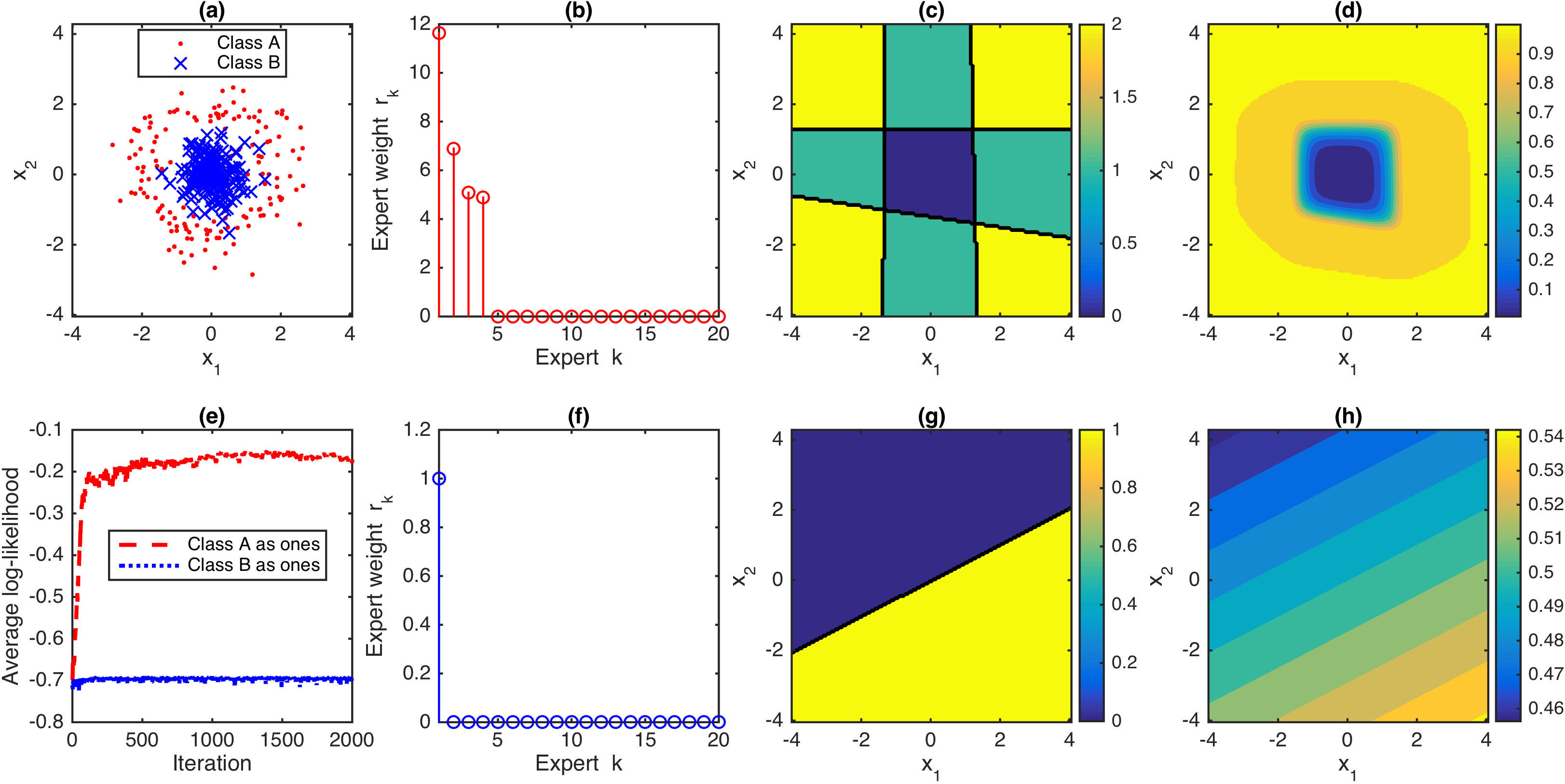
Figure 1: Visualization of sum-softplus regression with $K_{\max}=20$ experts on a binary classification problem under two opposite labeling settings. For each labeling setting, 2000 Gibbs sampling iterations are used and the MCMC sample that provides the maximum likelihood on fitting the training data labels is used to display the results. (a) A two dimensional dataset that consists of 150 data points from Class $A$, whose radiuses are drawn from $\mathcal{N}(2,0.5^{2})$ and angles are distributed uniformly at random between 0 and $360$ degrees, and another 150 data points from Class $B$, whose both $x$-axis and $y$-axis values are drawn from $\mathcal{N}(0,0.5^{2})$. With data points in Classes $A$ and $B$ labeled as “1” and “0,” respectively, and with $p_{0}=0.5$, (b) shows the inferred weights $r_{k}$ of the experts, ordered by their values, (c) shows a contour map, the value of each point of which represents how many inequalities specified in (17) are violated, and whose region with zero values corresponds to the convex polytope enclosed by the intersection of the hyperplanes defined in (17), and (d) shows the the contour map of the predicted class probabilities. (f)-(h) are analogous plots to (b)-(d), with the data points in Classes $A$ and $B$ relabeled as “0” and “1,” respectively. (e) The average per data point log-likelihood as a function of MCMC iteration, for both labeling settings.

Figure 2: Visualization of the posteriors of sum-softplus regression based on 20 MCMC samples, collected once per every 50 iterations during the last 1000 MCMC iterations, with the same experimental setting used for Fig. 1. With $p_{0}=0.5$, (a) and (b) show the contour maps of the posterior means and standard deviations, respectively, of the number of inequalities specified in (17) that are violated, and (c) and (d) show the contour maps of the posterior means and standard deviations, respectively, of predicted class probabilities. (e)-(h) are analogous plots to (a)-(d), with the data points in Classes $A$ and $B$ relabeled as “0” and “1,” respectively.

We first label the data points of Class $A$ as “1” and these of Class $B$ as “0.” Shown in Fig. 1 (b) are the inferred weights $r_{k}$ of the experts, using the MCMC sample that has the highest log-likelihood in fitting the training data labels. It is evident from Figs. 1 (b) and (c) that sum-softplus regression infers four experts (hyperplanes) with significant weights. The convex polytope in Fig. 1 (c) that encloses the space marked as zero is intersected by these four hyperplanes, each of which is defined as in (17) with $p_{0}=50\%$. Thus outside the convex polytope are data points that would be labeled as “1” with at least 50% probabilities and inside it are data points that would be labeled as “0” with relatively high probabilities. We further show in Fig. 1 (d) the contour map of the inferred probabilities for $P(y_{i}=1\,|\,\boldsymbol{x}_{i})=1-e^{-\lambda(\boldsymbol{x}_{i})}$, where $\lambda(\boldsymbol{x}_{i})$ are calculated with (8). Note that due to the model construction, a single expert’s influence on the decision boundary can be conveniently measured, and the exact decision boundary is bounded by a convex polytope. Thus it is not surprising that the convex polytope in Fig. 1 (c), which encloses the space marked as zero, aligns well with the contour line of $P(y_{i}=1\,|\,\boldsymbol{x}_{i})=0.5$ shown in Fig. 1 (d).

Despite being able to construct a nonlinear decision boundary bounded by a convex polytope, sum-softplus regression has a clear restriction in that if the data labels are flipped, its performance may substantially deteriorate, becoming no better than that of logistic regression. For example, for the same data shown in Fig. 1 (a), if we choose the opposite labeling setting where the data points of Class $A$ are labeled as “0” and these of Class $B$ are labeled as “1,” then sum-softplus regression infers a single expert (hyperplane) with non-negligible weight, as shown in Figs. 1 (f)-(g), and fails to separate the data points of two different classes, as shown in Figs. 1 (g)-(h). The data log-likelihood plots in Fig. 1 (e) also suggest that sum-softplus regression could perform substantially better if the training data are labeled in favor of its geometric constraints on the decision boundary. An advantage of a Bayesian hierarchical model is that with collected MCMC samples, one may estimate not only the posterior means but also uncertainties. The standard deviations shown in Figs. 2 (b) and (d) clearly indicate the uncertainties of sum-softplus regression on its decision boundaries and predictive probabilities in the covariate space, which may be used to help decide how to sequentially query the labels of unlabeled data in an active learning setting (Cohn et al., 1996; Settles, 2010).

The sensitivity of sum-softplus regression to how the data are labeled could be mitigated but not completely solved by combining two sum-softplus regression models trained under the two opposite labeling settings. In addition, sum-softplus regression may not perform well no matter how the data are labeled if neither of the two classes could be enclosed by a convex polytope. To fully resolve these issues, we first introduce stack-softplus regression, which defines a convex-polytope-like confined space to enclose positive examples. We then show how to combine the two distinct, but complementary, softplus regression models to construct SS-softplus regression that provides more flexible nonlinear decision boundaries.

2.5 Stack-softplus regression and stacked gamma distributions

The model in (11) combines the BerPo link with a gamma belief network that stacks differently parameterized gamma distributions. Note that here “stacking” is defined as an operation that mixes the shape parameter of a gamma distribution at layer $t$ with a gamma distribution at layer $t+1$, the next one pushed into the stack, and pops out the covariate-dependent gamma scale parameters from layers $T+1$ to 2 in the stack, following the last-in-first-out rule, to parameterize the BerPo rate of the class label $y_{i}$ shown in (10).

2.5.1 Convex-polytope-like confined space that favors positive examples

Let us make the analogy that each ${\boldsymbol{\beta}}^{(t)}$ is one of the $T$ criteria that an expert examines before making a binary decision. From (10) it is clear that as long as a single criterion $t\in\{2,\ldots,{T}+1\}$ of the expert is strongly violated, which means that $\boldsymbol{x}_{i}^{\prime}{\boldsymbol{\beta}}^{(t)}$ is much smaller than zero, then the expert would vote “No” regardless of the values of $\boldsymbol{x}_{i}^{\prime}{\boldsymbol{\beta}}^{({\tilde{t}})}$ for all ${\tilde{t}}\neq t$. Thus the response variable could be voted “Yes” by the expert only if none of the $T$ expert criteria are strongly violated. For stack-softplus regression, let us specify a confined space using the inequality $P(y_{i}=1\,|\,\boldsymbol{x}_{i})=1-e^{-\lambda(\boldsymbol{x}_{i})}>p_{0}$, which can be expressed as

$$\small\boldsymbol{x}_{i}^{\prime}{\boldsymbol{\beta}}^{({T}+1)}+\ln\ln\!\bigg{\{}1+e^{\boldsymbol{x}_{i}^{\prime}{\boldsymbol{\beta}}^{({T})}}\ln\Big{[}1+\ldots\ln\big{(}1+e^{\boldsymbol{x}_{i}^{\prime}{\boldsymbol{\beta}}^{(2)}}\big{)}\Big{]}\bigg{\}}>\ln\big{[}(1-p_{0})^{-\frac{1}{r}}-1\big{]},\vspace{0mm}$$ (18)

and hence any data point $\boldsymbol{x}_{i}$ outside the confined space ($i.e.$, violating the inequality in Eq. 18 a.s.) will be labeled as $y_{i}=0$ with a probability no less than $1-p_{0}$.

Considering the covariate space

$$\mathcal{T}^{-t}:=\left\{\boldsymbol{x}_{i}:\boldsymbol{x}^{\prime}_{i}{\boldsymbol{\beta}}_{{\tilde{t}}}\geq 0\text{ for }{\tilde{t}}\neq t\right\},\vspace{0mm}$$ (19)

where all the criteria except criterion $t$ of the expert tend to be satisfied, the decision boundary of stack-softplus regression in $\mathcal{T}^{-t}$ would be clearly influenced by the satisfactory level of criterion $t$, whose hyperplane partitions $\mathcal{T}^{-t}$ into two parts as

$$\small y_{i}=\begin{cases}\vspace{.15cm}\displaystyle 1,&{\mbox{if }}\displaystyle 1-\left(1^{T+1}+\ln\bigg{\{}1^{T}+\ln\Big{[}1^{T-1}+\ldots+\ln\big{(}1^{t}+e^{\boldsymbol{x}_{i}^{\prime}{\boldsymbol{\beta}}^{(t)}}g_{t-1}\big{)}\Big{]}\bigg{\}}\right)^{-r}\!\!>p_{0},\\ \displaystyle 0,&\mbox{otherwise},\end{cases}\vspace{0mm}$$ (20)

for all $\boldsymbol{x}_{i}\in\mathcal{T}^{-t}$. Let us define $g_{t}$ with $g_{1}=1$ and the recursion $g_{t}=\ln(1+g_{t-1})$ for $t=2,\ldots,T$, and define $h_{t}$ with $h_{T+1}=(1-p_{0})^{-\frac{1}{r}}-1$ and the recursion $h_{t}=e^{h_{t+1}}-1$ for $t=T,T-1,\ldots,2$. Using the definition of $g_{t}$ and $h_{t}$, combining all the $T$ expert criteria, the confined space of stack-softplus regression specified in (18) can be roughly related to a convex polytope, which is specified by the solutions to a set of $T$ inequalities as

$$\boldsymbol{x}_{i}^{\prime}{\boldsymbol{\beta}}^{(t)}>\ln(h_{t})-\ln(g_{t-1}),~{}t\in\{2,\ldots,T+1\}.$$ (21)

The convex polytope is enclosed by the intersection of $T$ $V$-dimensional hyperplanes, and since none of the $T$ criteria would be strongly violated inside the convex polytope, the label $y_{i}=1$ ($y_{i}=0$) would be assigned to an $\boldsymbol{x}_{i}$ inside (outside) the convex polytope with a relatively high (low) probability.

Unlike the confined space of sum-softplus regression defined in (16) that is bounded by a convex polytope defined in (17), the convex polytope defined in (21) only roughly corresponds to the confined space of stack-softplus regression, as defined in (18). Nevertheless, the confined space defined in (18) is referred to as a convex-polytope-like confined space, due to both its connection to the convex polytope in (21) and the fact that (18) is likely to be violated if at least one of the $T$ criteria is strongly dissatisfied ($i.e.$, $e^{\boldsymbol{x}_{i}^{\prime}{\boldsymbol{\beta}}^{(t)}}\rightarrow 0$ for some $t$).

2.5.2 Illustration for stack-softplus regression

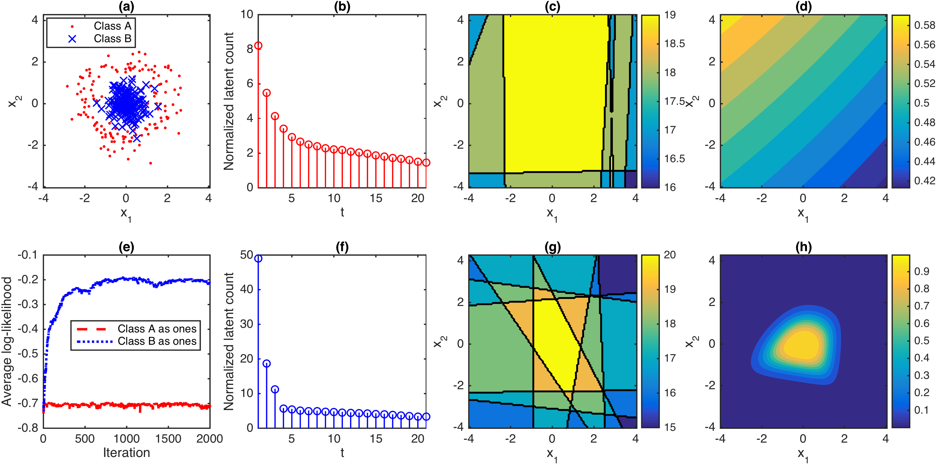
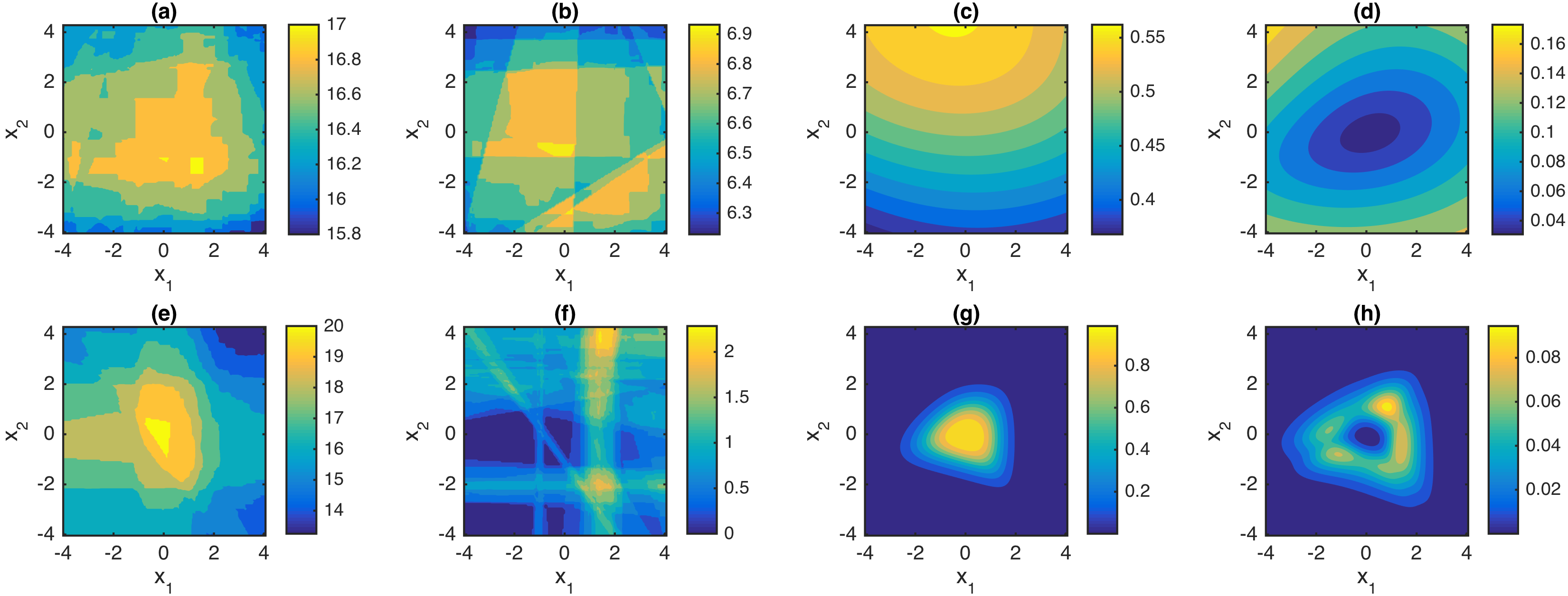
Figure 3: Analogous figure to Fig. 1 for stack-softplus regression with $T=20$ expert criteria, with the following differences: (b) shows the average latent count per positive sample, $\sum_{i}m_{i}^{(t)}\big{/}\sum_{i}\delta(y_{i}=1)$, as a function of layer $t$, (c) shows a contour map, the value of each point of which represents how many inequalities specified in (21) are satisfied, and whose region with the values of $T=20$ corresponds to the convex polytope enclosed by the intersections of the hyperplanes defined in (21),

Figure 4: Analogous figure to Fig. 2 for stack-softplus regression, with the following differences: (a) and (b) show the contour maps of the posterior means and standard deviations, respectively, of the number of inequalities specified in (21) that are satisfied. (e)-(f) are analogous plots to (a)-(b) under the opposite labeling setting.

Let us examine how stack-softplus regression performs on the same data used in Fig. 1. When Class $B$ is labeled as “1,” as shown in Fig. 4 (g), stack-softplus regression infers a convex polytope that encloses the space marked as $T=20$ using the intersection of all $T=20$ hyperplanes, each of which is defined as in (21); and as shown in Fig. 4 (h), it works well by using a convex-polytope-like confined space to enclose positive examples. However, as shown in Figs. 4 (c)-(e), its performance deteriorates when the opposite labeling setting is used. Note that due to the model construction that introduces complex interactions between the $T$ hyperplanes, (21) can only roughly describe how a single hyperplane could influence the decision boundary determined by all hyperplanes. Thus it is not surprising that neither the convex polytope in Fig. 4 (c), which encloses the space marked with the largest count there, nor the convex polytope in Fig. 4 (g), which encloses the space marked with $T$, align well with the contour lines of $P(y_{i}=1\,|\,\boldsymbol{x}_{i})=0.5$ in Figs. 4 (d) and (h), respectively.

While how the latent count $m_{\boldsymbol{\cdot}}^{(t)}$ decreases as $t$ increases does not indicate a clear cutoff point for the depth $T$, neither do we observe a clear sign of overfitting when $T$ is set as large as 100 in our experiments. Both Figs. 4 (c) and (g) indicate that most of the hyperplanes are far from any data points and tend to vote “Yes” for all training data. The standard deviations shown in Figs. 4 (f) and (h) clearly indicate the uncertainties of stack-softplus regression on its decision boundaries and predictive probabilities in the covariate space.

Like sum-softplus regression, stack-softplus regression also generalizes softplus and logistic regressions in that it uses the boundary of a confined space rather than a single hyperplane to partition the covariate space into two parts. Unlike the convex-polytope-bounded confined space of sum-softplus regression that favors placing negative examples inside it, the convex-polytope-like confined space of stack-softplus regression favors placing positive examples inside it. While both sum- and stack-softplus regressions could be sensitive to how the data are labeled, their distinct behaviors under the same labeling setting motivate us to combine them together as SS-softplus regression, as described below.

2.6 Sum-stack-softplus (SS-softplus) regression

Note that if ${T}=1$, SS-softplus regression reduces to sum-softplus regression; if $K=1$, it reduces to stack-softplus regression; and if $K=T=1$, it reduces to softplus regression, which further reduces to logistic regression if the weight of the single expert is fixed at $r=1$. To ensure that the SS-softplus regression model is well defined in its infinite limit, we provide the following proposition and present the proof in Appendix B.

Proposition 4.

The infinite product in sum-stack-softplus regression as

$$e^{-\sum_{k=1}^{\infty}r_{k}\,\varsigma\left(\boldsymbol{x}_{i}^{\prime}{\boldsymbol{\beta}}_{k}^{(2:T+1)}\right)}=\prod_{k=1}^{\infty}\left(\!1\!+\!e^{\boldsymbol{x}_{i}^{\prime}{\boldsymbol{\beta}}_{k}^{({T}\!+\!1)}}\ln\!\bigg{\{}1\!+\!e^{\boldsymbol{x}_{i}^{\prime}{\boldsymbol{\beta}}_{k}^{({T})}}\ln\Big{[}1\!+\!\ldots\ln\big{(}1\!+\!e^{\boldsymbol{x}_{i}^{\prime}{\boldsymbol{\beta}}_{k}^{(2)}}\big{)}\Big{]}\bigg{\}}\right)^{-r_{k}}$$

is smaller than one and has a finite expectation that is greater than zero.

2.6.1 Union of convex-polytope-like confined spaces

We may consider SS-softplus regression as a multi-hyperplane model that employs a committee, consisting of countably infinite experts, to make a decision, where each expert is equipped with $T$ criteria to be examined. The committee’s distribution is obtained by convolving the distributions of countably infinite experts, each of which mixes $T$ stacked covariate-dependent gamma distributions. For each $\boldsymbol{x}_{i}$, the committee votes “Yes” as long as at least one expert votes “Yes,” and an expert could vote “Yes” if and only if none of its $T$ criteria are strongly violated. Thus the decision boundary of SS-softplus regression can be considered as a union of convex-polytope-like confined spaces that all favor placing positively labeled data inside them, as described below, with the proofs deferred to Appendix B.

Theorem 5.

For sum-stack-softplus regression, the confined space specified by the inequality $P(y_{i}=1\,|\,\boldsymbol{x}_{i})=1-e^{-\lambda(\boldsymbol{x}_{i})}>p_{0}$, which can be expressed as

$$\lambda(\boldsymbol{x}_{i})=\sum_{k=1}^{\infty}r_{k}\,\varsigma\big{(}\boldsymbol{x}^{\prime}{\boldsymbol{\beta}}_{k}^{(2)},\ldots,\boldsymbol{x}^{\prime}{\boldsymbol{\beta}}_{k}^{(T+1)}\big{)}>-\ln(1-p_{0}),\vspace{0mm}$$ (22)

encompasses the union of convex-polytope-like confined spaces, expressed as

$$\mathcal{D}_{\star}=\mathcal{D}_{1}\cup\mathcal{D}_{2}\cup\ldots,$$

where the $k$th convex-polytope-like confined space $\mathcal{D}_{k}$ is specified by the inequality

$$\small\boldsymbol{x}_{i}^{\prime}{\boldsymbol{\beta}}_{k}^{({T}+1)}+\ln\ln\!\bigg{\{}1+e^{\boldsymbol{x}_{i}^{\prime}{\boldsymbol{\beta}}_{k}^{({T})}}\ln\Big{[}1+\ldots\ln\big{(}1+e^{\boldsymbol{x}_{i}^{\prime}{\boldsymbol{\beta}}_{k}^{(2)}}\big{)}\Big{]}\bigg{\}}>\ln\big{[}(1-p_{0})^{-\frac{1}{r_{k}}}-1\big{]}.\vspace{0mm}$$ (23)

Corollary 6.

For sum-stack-softplus regression, the confined space specified by the inequality $P(y_{i}=1\,|\,\boldsymbol{x}_{i})=1-e^{-\lambda(\boldsymbol{x}_{i})}\leq p_{0}$ is bounded by $\bar{\mathcal{D}}_{\star}=\bar{\mathcal{D}}_{1}\cap\bar{\mathcal{D}}_{2}\cap\ldots$

Proposition 7.

For any data point $\boldsymbol{x}_{i}$ that resides inside the union of countably infinite convex-polytope-like confined spaces $\mathcal{D}_{\star}=\mathcal{D}_{1}\cup\mathcal{D}_{2}\cup\ldots$, which means $\boldsymbol{x}_{i}$ satisfies at least one of the inequalities in (23), it will be labeled under sum-stack-softplus regression with $y_{i}=1$ with a probability greater than $p_{0}$, and $y_{i}=0$ with a probability no greater than $1-p_{0}$.

2.6.2 Illustration for sum-stack-softplus regression

Let us examine how SS-softplus regression performs on the same dataset used in Fig. 1. When Class $A$ is labeled as “1,” as shown in Figs. 6 (b)-(c), SS-softplus regression infers about eight convex-polytope-like confined spaces, the intersection of six of which defines the boundary of the covariate space that separates the points that violate all inequalities in (23) from the ones that satisfy at least one inequality in (23). The union of these convex-polytope-like confined spaces defines a confined covariate space, which is included within the covariate space satisfying $P(y_{i}\,|\,\boldsymbol{x}_{i})>0.5$, as shown in Fig. 6 (d).

When Class $B$ is labeled as “1,” as shown in Fig. 6 (f)-(g), SS-softplus regression infers about six convex-polytope-like confined spaces, one of which defines the boundary of the covariate space that separates the points that violate all inequalities in (23) from the others for the covariate space show in Fig. 6 (g). The union of two convex-polytope-like confined spaces defines a confined covariate space, which is included in the covariate space with $P(y_{i}\,|\,\boldsymbol{x}_{i})>0.5$, as shown in Fig. 6 (h). Figs. 6 (f)-(g) also indicate that except for two convex-polytope-like confined spaces, the boundaries of all the other convex-polytope-like confined spaces are far from any data points and tend to vote “No” for all training data. The standard deviations shown in Figs. 6 (b), (d), (f), and (h) clearly indicate the uncertainties of SS-softplus regression on classification decision boundaries and predictive probabilities.

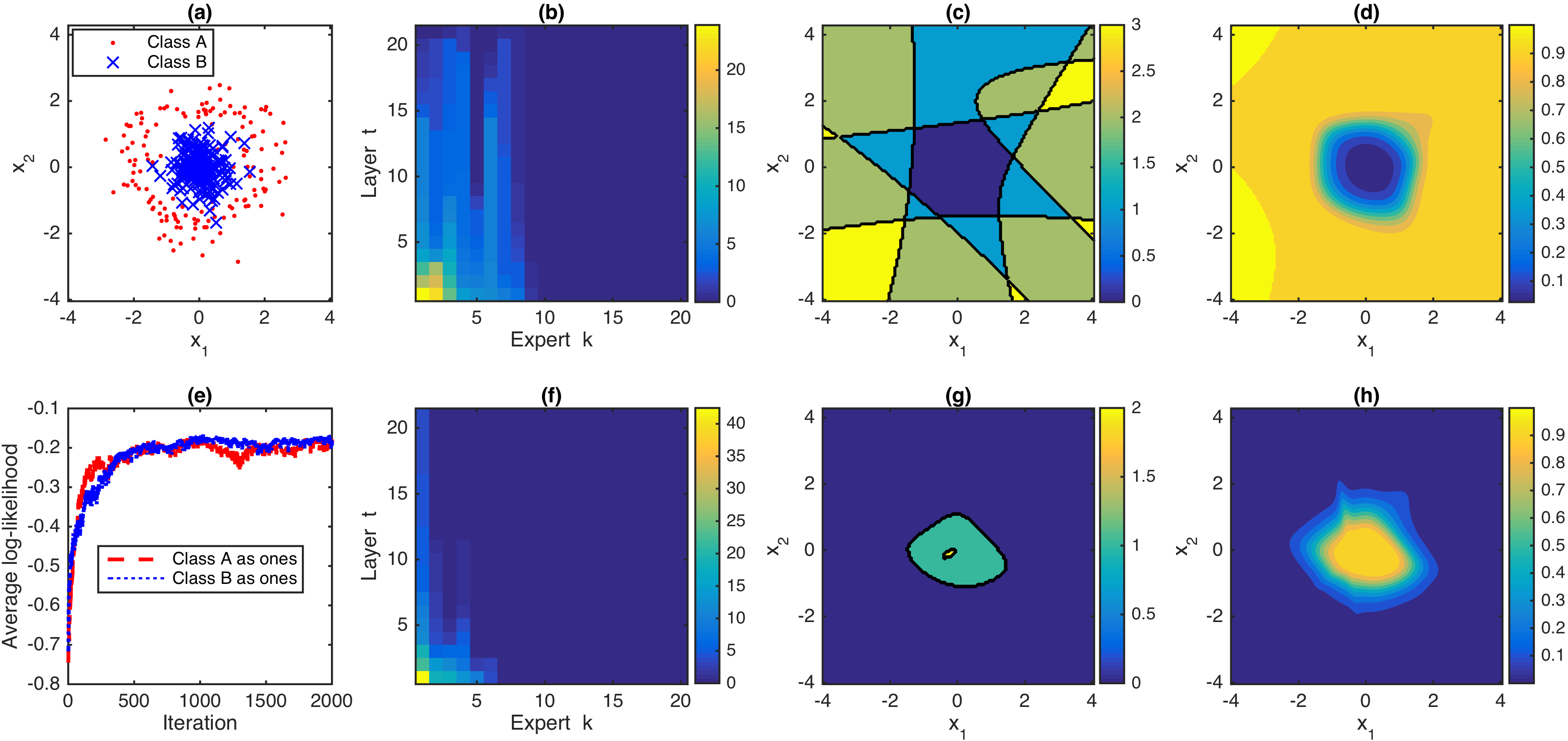
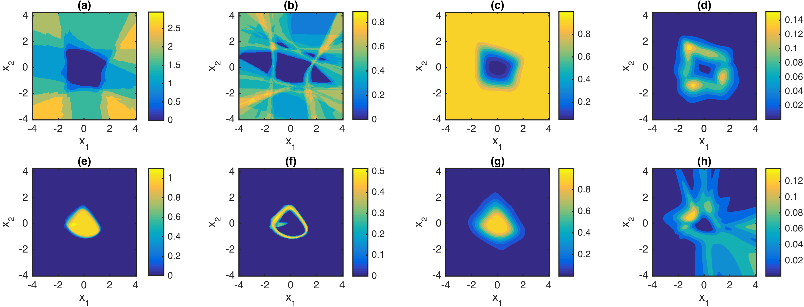
Figure 5: Analogous figure to Figs. 1 and 4 for SS-softplus regression with $K_{\max}=20$ experts and $T=20$ criteria for each expert, with the following differences: (b) shows the average latent count per positive sample, $\sum_{i}m_{ik}^{(t)}\big{/}\sum_{i}\delta(y_{i}=1)$, as a function of both the expert index $k$ and layer index $t$, where the experts are ordered based on the values of $\sum_{i}m_{ik}^{(1)}$, (c) shows a contour map, the value of each point of which represents how many inequalities specified in (23) are satisfied, and whose region with nonzero values corresponds to the union of convex-polytope-like confined spaces, each of which corresponds to an inequality defined in (23), and (f) and (g) are analogous plots to (b) and (c) under the opposite labeling setting where data in Class $B$ are labeled as “1.”

Figure 6: Analogous figure to Fig. 2 for SS-softplus regression, with the following differences: (a) and (b) show the contour maps of the posterior means and standard deviations, respectively, of the number of inequalities specified in (23) that are satisfied. (e)-(f) are analogous plots to (a)-(b).

3 Gibbs sampling via data augmentation and marginalization

Since logistic, softplus, sum-softplus, and stack-softplus regressions can all be considered as special cases of SS-softplus regression, below we will focus on presenting the nonparametric Bayesian hierarchical model and Bayesian inference for SS-softplus regression.

The gamma process $G\sim\Gamma{\mbox{P}}(G_{0},1/c)$ has an inherent shrinkage mechanism, as in the prior the number of atoms with weights larger than $\epsilon>0$ follows $\mbox{Pois}\left(\gamma_{0}\int_{\epsilon}^{\infty}r^{-1}e^{-cr}dr\right),$ whose mean is finite a.s., where $\gamma_{0}=G_{0}(\Omega)$ is the mass parameter of the gamma process. In practice, the atom with a tiny weight generally has a negligible impact on the final decision boundary of the model, hence one may truncate either the weight to be above $\epsilon$ or the number of atoms to be below $K$. One may also follow Wolpert et al. (2011) to use a reversible jump MCMC (Green, 1995) strategy to adaptively truncate the number of atoms for a gamma process, which often comes with a high computational cost. For the convenience of implementation, we truncate the number of atoms in the gamma process to be $K$ by choosing a finite discrete base measure as $G_{0}=\sum_{k=1}^{K}\frac{\gamma_{0}}{K}\delta_{\alpha_{k}}$, where $K$ will be set sufficiently large to achieve a good approximation to the truly countably infinite model.

We express the truncated SS-softplus regression model using (13) together with

$$r_{k}\sim\mbox{Gamma}(\gamma_{0}/K,1/c_{0}),~{}\gamma_{0}\sim\mbox{Gamma}(a_{0},1/b_{0}),~{}c_{0}\sim\mbox{Gamma}(e_{0},1/f_{0}),$$

$$~{}~{}~{}~{}~{}~{}~{}~{}~{}~{}~{}~{}~{}~{}~{}~{}~{}{\boldsymbol{\beta}}^{(t)}_{k}\sim\prod_{v=0}^{V}\mathcal{N}(0,\alpha_{vtk}^{-1}),~{}\alpha_{vtk}\sim\mbox{Gamma}(a_{t},1/b_{t}),$$ (24)

where $t\in\{2,\ldots,T+1\}$. Related to Tipping (2001), the normal gamma construction in (24) is used to promote sparsity on the regression coefficients ${\boldsymbol{\beta}}^{(t)}_{k}$. We derive Gibbs sampling by exploiting local conjugacies under a series of data augmentation and marginalization techniques. We comment here that while the proposed Gibbs sampling algorithm is a batch learning algorithm that processes all training data samples in each iteration, the local conjugacies revealed under data augmentation and marginalization may be of significant value in developing efficient mini-batch based online learning algorithms, including those based on stochastic gradient MCMC (Welling and Teh, 2011; Girolami and Calderhead, 2011; Patterson and Teh, 2013; Ma et al., 2015) and stochastic variation inference (Hoffman et al., 2013). We leave the maximum likelihood, maximum a posteriori, (stochastic) variational Bayes inference, and stochastic gradient MCMC for softplus regressions for future research.

For a model with ${T}=1$, we exploit the data augmentation techniques developed for the BerPo link in Zhou (2015) to sample $m_{i}$, these developed for the Poisson and multinomial distributions (Dunson and Herring, 2005; Zhou et al., 2012a) to sample $m_{ik}$, these developed for the NB distribution in Zhou and Carin (2015) to sample $r_{k}$ and $\gamma_{0}$, and these developed for logistic regression in Polson and Scott (2011) and further generalized to NB regression in Zhou et al. (2012b) and Polson et al. (2013) to sample ${\boldsymbol{\beta}}_{k}$. We exploit local conjugacies to sample all the other model parameters. For a model with ${T}\geq 2$, we further generalize the inference technique developed for the gamma belief network in Zhou et al. (2015a) to sample the model parameters of deep hidden layers. Below we provide a theorem, related to Lemma 1 for the gamma belief network in Zhou et al. (2015a), to show that each regression coefficient vector can be linked to latent counts under NB regression. Let $m\sim\mbox{SumLog}(n,p)$ represent the sum-logarithmic distribution described in Zhou et al. (2015b), Corollary 9 further shows an alternative representation of (13), the hierarchical model of SS-softplus regression, where all the covariate-dependent gamma distributions are marginalized out.

Theorem 8.

Let us denote $p_{ik}^{(t)}=1-e^{-{q}_{ik}^{(t)}}$, $i.e.$, ${q}_{ik}^{(t)}=-\ln(1-p_{ik}^{(t)})$, and $\theta_{ik}^{({T}+1)}=r_{k}$. With ${q}_{ik}^{(1)}:=1$ and

$${q}_{ik}^{(t+1)}:=\ln\left(1+{q}_{ik}^{(t)}e^{\boldsymbol{x}_{i}{\boldsymbol{\beta}}_{k}^{(t+1)}}\right)\vspace{0mm}$$ (25)

for $t=1,\ldots,T$, which means

$${q}_{ik}^{(t+1)}=\varsigma\big{(}\boldsymbol{x}_{i}^{\prime}{\boldsymbol{\beta}}_{k}^{(2)},\ldots,\boldsymbol{x}_{i}^{\prime}{\boldsymbol{\beta}}_{k}^{(t+1)}\big{)}$$

$$= \displaystyle\ln\left(\!1\!+\!e^{\boldsymbol{x}_{i}^{\prime}{\boldsymbol{\beta}}_{k}^{({t}\!+\!1)}}\ln\!\bigg{\{}1\!+\!e^{\boldsymbol{x}_{i}^{\prime}{\boldsymbol{\beta}}_{k}^{({t})}}\ln\Big{[}1\!+\!\ldots\ln\big{(}1\!+\!e^{\boldsymbol{x}_{i}^{\prime}{\boldsymbol{\beta}}_{k}^{(2)}}\big{)}\Big{]}\bigg{\}}\right),\vspace{0mm}$$ (26)

one may find latent counts $m_{ik}^{(t)}$ that are connected to the regression coefficient vectors as

$$m_{ik}^{(t)}\sim\emph{\mbox{NB}}(\theta_{ik}^{(t+1)},~{}~{}1-e^{-{q}_{ik}^{(t+1)}})=\emph{\mbox{NB}}\left(\theta_{ik}^{(t+1)},\frac{1}{1+e^{-\boldsymbol{x}_{i}^{\prime}{\boldsymbol{\beta}}_{k}^{(t+1)}-\ln({q}_{ik}^{(t)})}}\right).\vspace{0mm}$$ (27)

Corollary 9.

With $q_{ik}^{(t)}=-\ln(1-p_{ik}^{(t)})$ defined as in (26) and hence $p_{ik}^{(t)}=1-e^{-q_{ik}^{(t)}}$, the hierarchical model of sum-stack-softplus regression can also be expressed as

$$m_{ik}^{(T+1)}\sim\emph{\mbox{Pois}}(r_{k}q_{ik}^{(T+1)}),~{}r_{k}\sim\emph{\mbox{Gamma}}(\gamma_{0}/K,1/c_{0}),$$

$$m_{ik}^{(T)}\sim\emph{\mbox{SumLog}}(m_{ik}^{(T+1)},p_{ik}^{(T+1)}),~{}{\boldsymbol{\beta}}^{({T}+1)}_{k}\sim\prod_{v=0}^{V}\mathcal{N}(0,\alpha_{v({T}+1)k}^{-1}),$$

$$~{}~{}~{}~{}~{}~{}~{}~{}~{}~{}~{}~{}~{}~{}~{}~{}~{}~{}~{}~{}~{}~{}~{}~{}~{}~{}~{}~{}~{}~{}~{}~{}~{}\tiny{\cdots}$$

$$m_{ik}^{(t)}\sim\emph{\mbox{SumLog}}(m_{ik}^{(t+1)},p_{ik}^{(t+1)}),~{}{\boldsymbol{\beta}}^{(t+1)}_{k}\sim\prod_{v=0}^{V}\mathcal{N}(0,\alpha_{v(t+1)k}^{-1}),$$

$$~{}~{}~{}~{}~{}~{}~{}~{}~{}~{}~{}~{}~{}~{}~{}~{}~{}~{}~{}~{}~{}~{}~{}~{}~{}~{}~{}~{}~{}~{}~{}~{}~{}\tiny{\cdots}$$

$$y_{i}=\delta(m_{i} \geq 1),~{}m_{i}=\sum_{k=1}^{K}m^{(1)}_{ik},~{}m^{(1)}_{ik}\sim\emph{\mbox{SumLog}}(m_{ik}^{(2)},p_{ik}^{(2)}),~{}{\boldsymbol{\beta}}^{(2)}_{k}\sim\prod_{v=0}^{V}\mathcal{N}(0,\alpha_{v2k}^{-1}),$$ (28)

We outline Gibbs sampling in Algorithm 1 of Appendix E, where to save computation, we consider setting $K_{\max}$ as the upper-bound of the number of experts and deactivating experts assigned with zero counts during MCMC iterations. We provide several additional model properties in Appendix C.2 to describe how the latent counts propagate across layers, which may be used to decide how to set the number of layers $T$. For simplicity, we consider the number of criteria for each expert as a parameter that determines the model capacity and we fix it as $T$ for all experts in this paper. We defer the details of all Gibbs sampling update equations to Appendix C, in which we also describe in detail how to ensure numerical stability in a finite precision machine. Note that except for the sampling of $\{m^{(1)}_{ik}\}_{k}$, the sampling of all the other parameters of different experts are embarrassingly parallel.

4 Example Results

We compare softplus regressions with logistic regression, Gaussian radial basis function (RBF) kernel support vector machine (SVM) (Boser et al., 1992; Vapnik, 1998; Schölkopf et al., 1999), relevance vector machine (RVM) (Tipping, 2001), adaptive multi-hyperplane machine (AMM) (Wang et al., 2011), and convex polytope machine (CPM) (Kantchelian et al., 2014). Except for logistic regression that is a linear classifier, both kernel SVM and RVM are widely used nonlinear classifiers relying on the kernel trick, and both AMM and CPM use the intersection of multiple hyperplanes to construct their decision boundaries. We discuss the connections between softplus regressions and previous work in Appendix D.

Following Tipping (2001), we consider the following datasets: banana, breast cancer, titanic, waveform, german, and image. For each of these six datasets, we consider the first ten predefined random training/testing partitions, and report both the mean and standard deviation of the testing classification errors. Since these datasets, originally provided by Rätsch et al. (2001), were no longer available on the authors’ websites, we use the version provided by Diethe (2015). We also consider two additional datasets—ijcnn1 and a9a—that come with a default training/testing partition, for which we report the results of logistic regression, SVM, and RVM based on a single trial, and report the results of all the other algorithms based on five independent trials with different random initiations. We summarize in Tab. 6 of Appendix E the basic information of these benchmark datasets.

Since the decision boundaries of all softplus regressions depend on whether the two classes are labeled as “1” and “0” or labeled as “0” and “1,” we consider repeating the same softplus regression algorithm twice, using both $y_{i1}\sim\mbox{BerPo}[\lambda_{1}(\boldsymbol{x}_{i})]\text{ and }y_{i2}\sim\mbox{BerPo}[\lambda_{2}(\boldsymbol{x}_{i})],$ where $y_{i1}$ and $y_{i2}:=1-y_{i1}$ are the labels under two opposite labeling settings. We combine them to the following predictive distribution $y_{i}\,|\,\boldsymbol{x}_{i}\sim\mbox{Bernoulli}\left[(1-e^{-\lambda_{1}(\boldsymbol{x}_{i})}+e^{-\lambda_{2}(\boldsymbol{x}_{i})})/2\right],$ which no longer depends on how the data are labeled. If we set $p_{0}=0.5$ as the probability threshold to make binary decisions, then $y_{i}$ would be labeled as “1” if $\lambda_{1}(\boldsymbol{x}_{i})>\lambda_{2}(\boldsymbol{x}_{i})$ and labeled as “0” otherwise. This simple strategy to train the same asymmetric model under two opposite labeling settings and combine their results together is related to the one used in Kantchelian et al. (2014), which, however, lacks of probabilistic interpretation. We leave more sophisticated training and combination strategies to future study.

For all datasets, we consider 1) softplus regression, which generalizes logistic regression with $r\neq 1$, 2) sum-softplus regression, which reduces to softplus regression if the number of experts is $K=1$, 3) stack-softplus regression, which reduces to softplus regression if the number of layers is $T=1$, and 4) sum-stack-softplus (SS-softplus) regression, which reduces to sum-softplus regression if $T=1$, to stack-softplus regression if $K=1$, and to softplus regression if $K=T=1$. For sum-softplus regresion, we set the upperbound on the number of experts as $K_{\max}=20$, for deep softplus regression, we consider $T\in\{1,2,3,5,10\}$, and for SS-softplus regression, we set $K_{\max}=20$ and consider $T\in\{1,2,3,5,10\}$. For all softplus regressions, we consider 5000 Gibbs sampling iterations and record the maximum likelihood sample found during the last 2500 iterations as the point estimates of $r_{k}$ and ${\boldsymbol{\beta}}_{k}^{(t)}$, which are used for out-of-sample predictions. We set $a_{0}=b_{0}=0.01$, $e_{0}=f_{0}=1$, and $a_{t}=b_{t}=10^{-6}$ for $t\in\{2,\ldots,T+1\}$. As in Algorithm 1 shown in Appendix E, we deactivate inactive experts for iterations in $I_{Prune}=\{525,575,\ldots,4975\}$. For a fair comparison, to ensure that the same training/testing partitions are used for all algorithms for all datasets, we report the results by using either widely used open-source software packages or the code made public available by the original authors. We describe in Appendix E the settings of all the algorithms that are used for comparison.

4.1 Illustrations

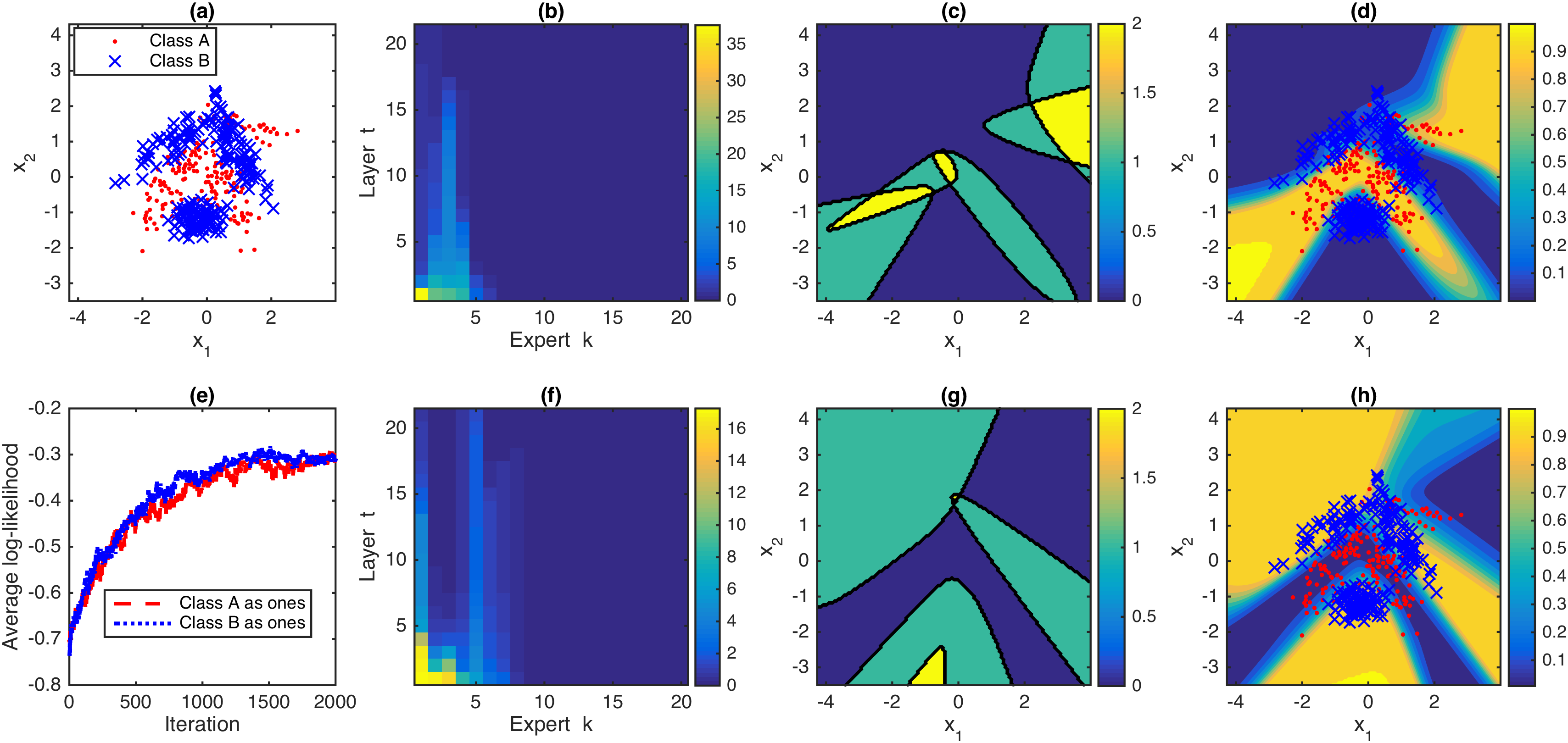
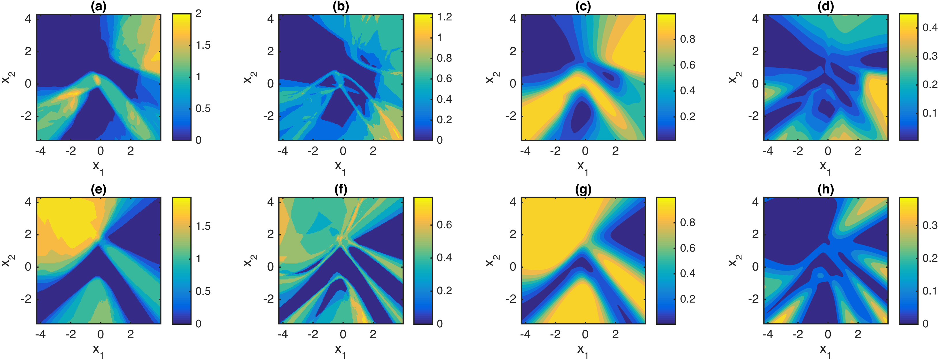
Figure 7: Analogous figure to Fig. 6 for the “banana” dataset.

Figure 8: Analogous figure to Fig. 6 for the “banana” dataset.

With a synthetic dataset, Figs. 1-6 illustrate the distinctions and connections between the sum-, stack-, and SS-softplus regressions. While both sum- and stack-softplus could work well for the synthetic dataset if the two classes are labeled in their preferred ways, as shown in Figs. 1 and 4, SS-softplus regression, as shown in Fig. 6, works well regardless of how the data are labeled. To further illustrate how the distinct, but complementary, behaviors of the sum- and stack-softplus regressions are combined together in SS-softplus regression, let us examine how SS-softplus regression performs on the banana dataset shown in Fig. 8 (a). When Class $A$ is labeled as “1,” as shown in Figs. 8 (b)-(c), SS-softplus regression infers about six convex-polytope-like confined spaces, the intersection of five of which defines the boundary of the covariate space that separates the points that satisfy at least one inequality in (23) from the ones that violate all inequalities in (23). The union of these convex-polytope-like confined spaces defines a confined covariate space, which is included within the covariate space satisfying $P(y_{i}\,|\,\boldsymbol{x}_{i})>0.5$, as shown in Fig. 8 (d).

When Class $B$ is labeled as “1,” as shown in Fig. 8 (f)-(g), SS-softplus regression infers about eight convex-polytope-like confined spaces, three of which define the boundary of the covariate space that separates the points that satisfy at least one inequality in (23) from the others for the covariate space show in Fig. 8 (g). The union of four convex-polytope-like confined spaces defines a confined covariate space, which is included in the covariate space with $P(y_{i}\,|\,\boldsymbol{x}_{i})>0.5$, as shown in Fig. 8 (h). Figs. 8 (f)-(g) also indicate that except for four convex-polytope-like confined spaces, all the other inferred convex-polytope-like confined spaces are far away from and tend to vote “No” for all training data. The standard deviations shown in Figs. 8 (b), (d), (f), and (h) indicate the uncertainties of SS-softplus regression on classification decision boundaries and predictive probabilities in the covariate space.

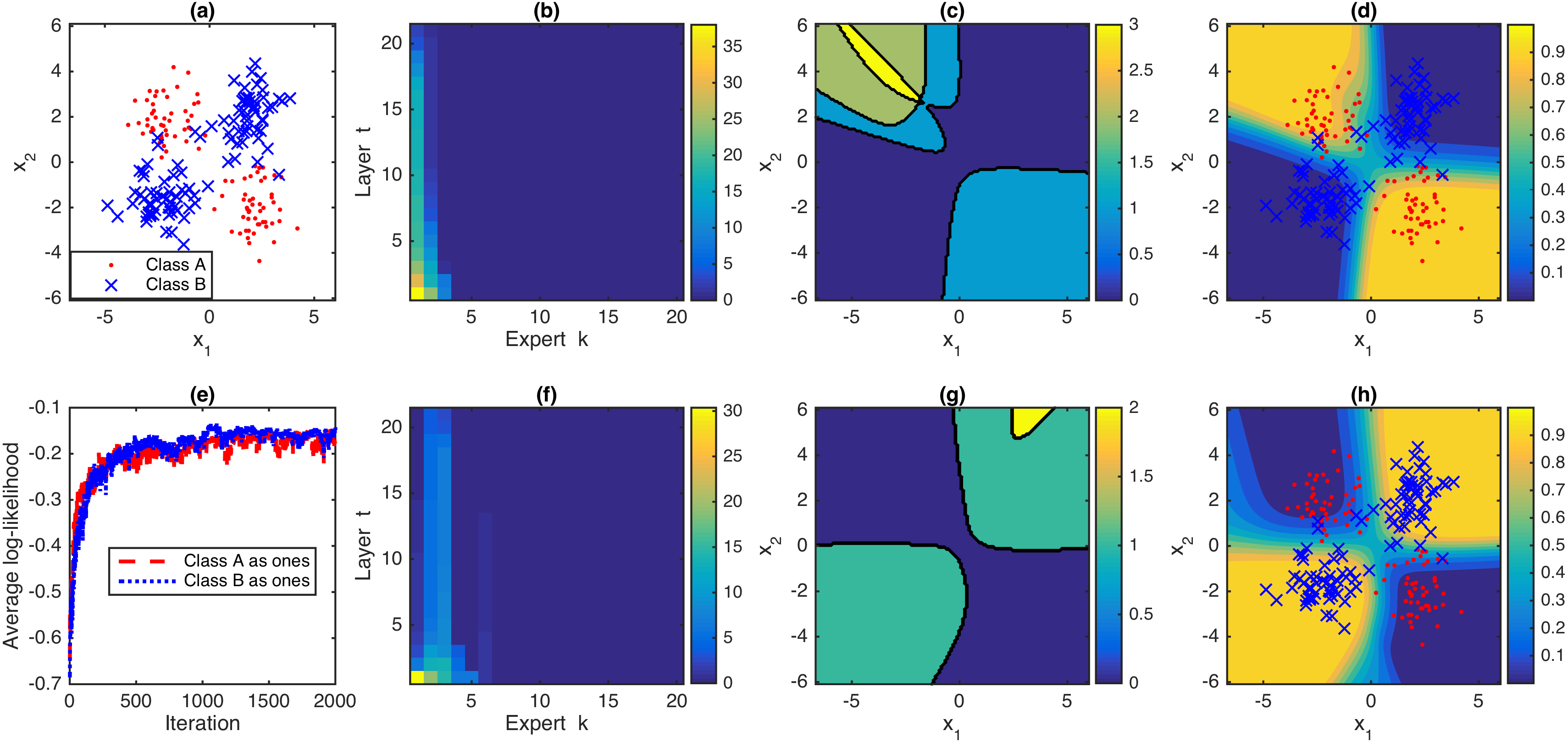
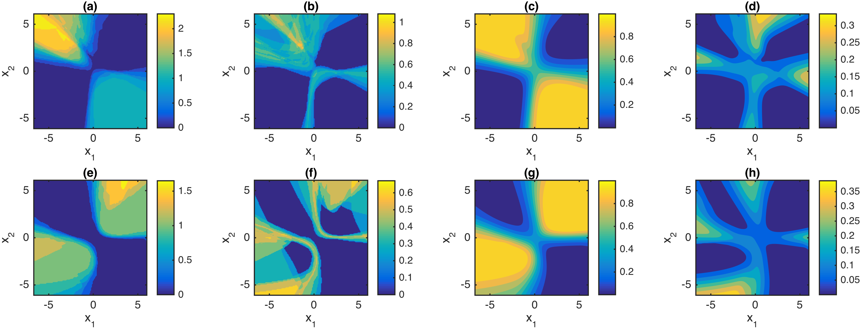
Figure 12: Analogous figure to to Fig. 8 for SS-softplus regression for a different dataset with two classes, where Class $A$ consists of 50 data points $(x_{i},y_{i})$ centering around $(-2,2)$, where $x_{i}\sim\mathcal{N}(-2,1)$ and $y_{i}\sim\mathcal{N}(2,1)$, and another 50 such kind of data points centering around $(2,-2)$, and Class $B$ consists of 50 such kind of data points centering around $(2,2)$ and another 50 such kind of data points centering around $(-2,-2)$.

Figure 13: Analogous figure to Fig. 8, with the same experimental setting used for Fig. 13.

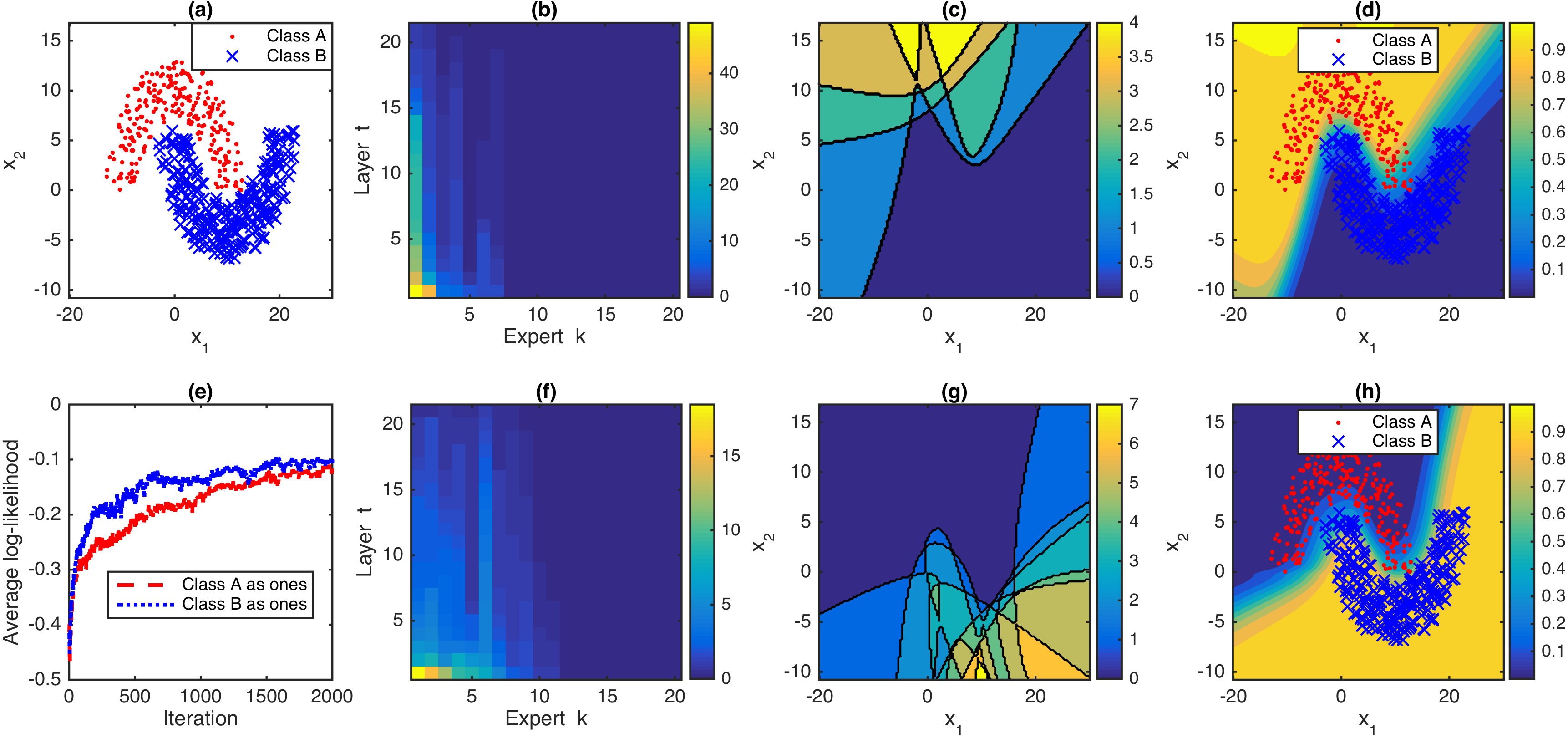
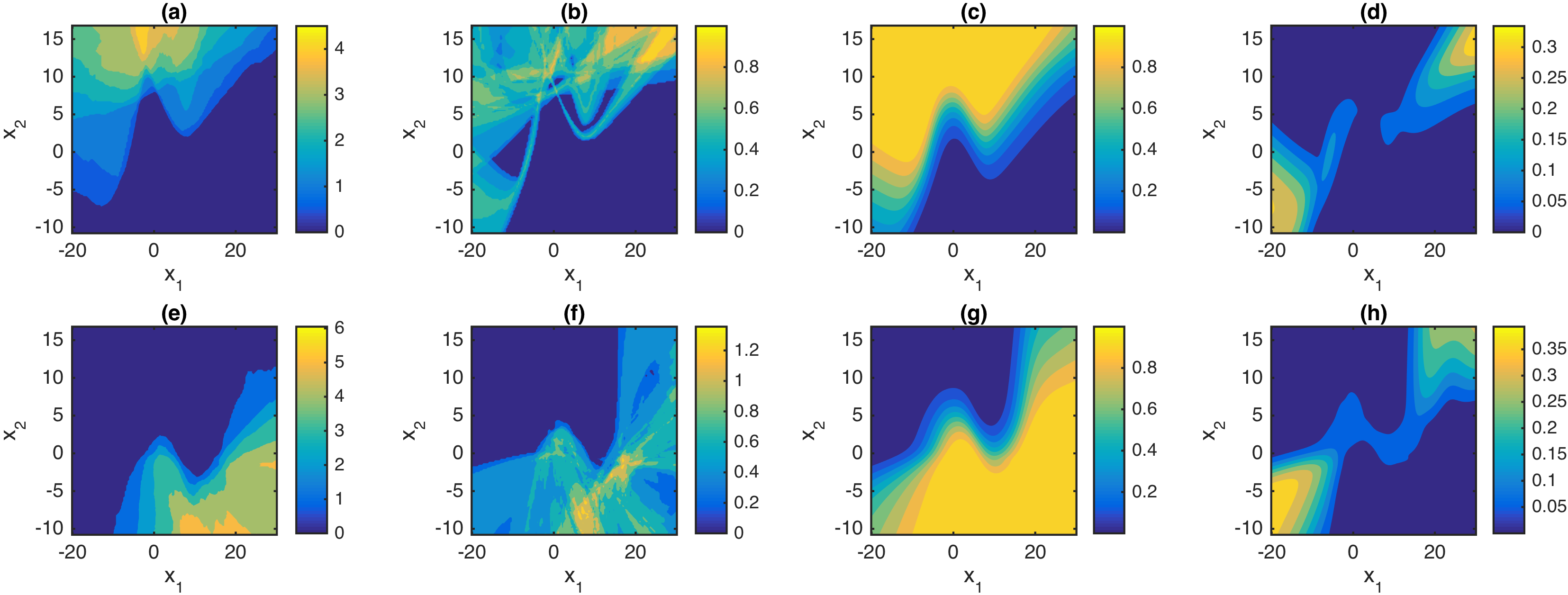
Figure 14: Analogous figure to Fig. 8 for SS-softplus regression for a double moon dataset, where both Classes $A$ and $B$ consist of 250 data points $(x_{i},y_{i})$.

Figure 15: Analogous figure to Fig. 8, with the same experimental setting used for Fig. 15.

In Figs. 13-15 of Appendix E, we further illustrate SS-softplus regression on an exclusive-or (XOR) dataset and a double-moon dataset used in Haykin (2009). For the banana, XOR, and double-moon datasets, where the two classes cannot be well separated by a single convex-polytope-like confined space, neither sum- nor stack-softplus regressions work well regardless of how the data are labeled, whereas SS-softplus regression infers the union of multiple convex-polytope-like confined spaces that successfully separates the two classes.

4.2 Classification performance on benchmark data

Table 1: Comparison of classification errors of logistic regression (LR), RBF kernel support vector machine (SVM), relevance vector machine (RVM), adaptive multi-hyperplane machine (AMM), convex polytope machine (CPM), softplus regression, sum-softplus (sum-$\varsigma$) regression with $K_{\max}=20$, stack-softplus (stack-$\varsigma$) regression with $T=5$, and SS-softplus (SS-$\varsigma$) regression with $K_{\max}=20$ and $T=5$. Displayed in each column of the last row is the average of the classification errors of an algorithm normalized by those of kernel SVM.

Dataset	LR	SVM	RVM	AMM	CPM	​softplus	​ sum-$\varsigma$​	​​stack-$\varsigma$ ($T$=5)​	​​SS-$\varsigma$ ($T$=5)
banana	$47.76$	$\mathbf{10.85}$	$11.08$	$18.76$	$21.39$	$47.87$	$30.78$	$33.21$	$11.89$
	$\pm 4.38$	$\pm 0.57$	$\pm 0.69$	$\pm 4.09$	$\pm 1.72$	$\pm 4.36$	$\pm 8.68$	$\pm 5.76$	$\pm 0.61$
breast	$28.05$	$28.44$	$31.56$	$31.82$	$32.08$	$28.70$	$30.13$	$\mathbf{27.92}$	$28.83$
cancer	$\pm 3.68$	$\pm 4.52$	$\pm 4.66$	$\pm 4.47$	$\pm 4.29$	$\pm 4.76$	$\pm 4.23$	$\pm 3.31$	$\pm 3.40$
titanic	$22.67$	$22.33$	$23.20$	$28.85$	$22.37$	$22.53$	$22.48$	$22.71$	$\mathbf{22.29}$
	$\pm 0.98$	$\pm 0.63$	$\pm 1.08$	$\pm 8.56$	$\pm 0.45$	$\pm 0.43$	$\pm 0.25$	$\pm 0.70$	$\pm 0.80$
waveform	$13.33$	$\mathbf{10.73}$	$11.16$	$11.81$	$12.76$	$13.62$	$11.51$	$12.25$	$11.69$
	$\pm 0.59$	$\pm 0.86$	$\pm 0.72$	$\pm 1.13$	$\pm 1.17$	$\pm 0.71$	$\pm 0.65$	$\pm 0.69$	$\pm 0.69$
german	$23.63$	$23.30$	$23.67$	$25.13$	$25.03$	$24.07$	$23.60$	$\mathbf{22.97}$	$24.23$
	$\pm 1.70$	$\pm 2.51$	$\pm 2.28$	$\pm 3.73$	$\pm 2.49$	$\pm 2.11$	$\pm 2.39$	$\pm 2.22$	$\pm 2.46$
image	$17.53$	$2.84$	$3.82$	$3.82$	$3.25$	$17.55$	$3.50$	$7.97$	$\mathbf{2.73}$
	$\pm 1.05$	$\pm 0.52$	$\pm 0.59$	$\pm 0.87$	$\pm 0.41$	$\pm 0.75$	$\pm 0.73$	$\pm 0.52$	$\pm 0.53$
Mean of SVM normalized errors	$2.472$	$1$	$1.095$	$1.277$	$1.251$	$2.485$	$1.370$	$1.665$	$1.033$

Table 2: Analogous table to Tab. 2 for comparing the number of experts (times the number of hyperplanes per expert), where an expert contains $T$ hyperplanes for both stack- and SS-softplus regressions and contains a single hyperplane/support vector for all the others. The computational complexity for out-of-sample prediction is about linear in the number of hyperplanes/support vectors. Displayed in each column of the last row is the average of the number of experts (times the number of hyperplanes per expert) of an algorithm normalized by those of RBF kernel SVM.

Dataset	LR	SVM	RVM	AMM	CPM	softplus	sum-$\varsigma$	stack-$\varsigma$​ ($T$=5)	SS-$\varsigma$​ ($T$=5)
banana	$1$	$129.20$	$22.30$	$9.50$	$14.60$	$2$	$3.70$	$2~{}(\times 5)$	$7.60~{}(\times 5)$
		$\pm 32.76$	$\pm 26.02$	$\pm 2.80$	$\pm 7.49$		$\pm 0.95$		$\pm 1.17~{}(\times 5)$
breast	$1$	$115.10$	$24.80$	$13.40$	$12.00$	$2$	$3.10$	$2~{}(\times 5)$	$6.40~{}(\times 5)$
cancer		$\pm 11.16$	$\pm 28.32$	$\pm 0.84$	$\pm 8.43$		$\pm 0.74$		$\pm 1.43~{}(\times 5)$
titanic	$1$	$83.40$	$5.10$	$14.90$	$5.20$	$2$	$2.30$	$2~{}(\times 5)$	$4.00~{}(\times 5)$
		$\pm 13.28$	$\pm 3.03$	$\pm 3.14$	$\pm 2.53$		$\pm 0.48$		$\pm 0.94~{}(\times 5)$
waveform	$1$	$147.00$	$21.10$	$9.50$	$6.40$	$2$	$4.40$	$2~{}(\times 5)$	$8.90~{}(\times 5)$
		$\pm 38.49$	$\pm 10.98$	$\pm 1.18$	$\pm 2.27$		$\pm 0.84$		$\pm 2.33~{}(\times 5)$
german	$1$	$423.60$	$11.00$	$18.80$	$8.80$	$2$	$6.70$	$2~{}(\times 5)$	$14.70~{}(\times 5)$
		$\pm 55.02$	$\pm 3.20$	$\pm 1.81$	$\pm 7.79$		$\pm 0.95$		$\pm 1.77~{}(\times 5)$
image	$1$	$211.60$	$35.80$	$10.50$	$23.00$	$2$	$11.20$	$2~{}(\times 5)$	$17.60~{}(\times 5)$
		$\pm 47.51$	$\pm 9.19$	$\pm 1.08$	$\pm 6.75$		$\pm 1.32$		$\pm 1.90~{}(\times 5)$
Mean of SVM normalized $K$	$0.007$	$1$	$0.131$	$0.088$	$0.075$	$0.014$	$0.030$	$0.014~{}(\times 5)$	$0.057~{}(\times 5)$

We summarize in Tab. 2 the results for the first six benchmark datasets described in Tab. 6, for each of which we report the results based on the first ten predefined random training/testing partitions. Overall for these six datasets, the RBF kernel SVM has the highest average out-of-sample prediction accuracy, followed closely by SS-softplus regression, whose mean of the errors normalized by these of of the SVM is as small as 1.033, and then by RVM, whose mean of normalized errors is 1.095. Overall, logistic regression does not perform well, which is not surprising as it is a linear classifier that uses a single hyperplane to partition the covariate space into two halves to separate one class from the other. Softplus regression, which uses an additional parameter over logistic regression, fails to reduce the classification errors of logistic regression; both sum-softplus regression, a multi-hyperplane generalization using the convolution operation, and stack-softplus regression, a multi-hyperplane generalization using the stacking operation, clearly reduce the classification errors; and SS-regression that combines both the convolution and stacking operations further improves the overall performance. Both CPM and AMM perform similarly to sum-softplus regression, which is not surprising given their connections discussed in Appendix D.2.

For out-of-sample prediction, the computation of a classification algorithm generally increases linearly in the number of used hyperplanes or support vectors. We summarize the number of experts (times the number of hyperplanes per expert if that number is not one) in Tab. 2, which indicates that in comparison to SVM that consistently requires the most number of experts (each expert corresponds to a support vector for SVM), the RVM, AMM, CPM, and the three proposed multi-hyperplane softplus regressions all require significantly less time for predicting the class label of a new data sample. It is also interesting to notice that the number of hyperplanes automatically inferred from the data by sum-softplus regression is generally smaller than the ones of AMM and CPM, both of which are selected through cross validations. Note that the number of active experts, defined as the value of $\sum_{k}\delta(\sum_{i}m^{(1)}_{ik}>0)$, inferred by both sum- and SS-softplus regressions shown in Tab. 2 will be further reduced if we only take into consideration the experts whose weights are larger than a certain threshold, such as those with $r_{k}>0.001$ for $k\in\{1,\ldots,K_{\max}\}$.

Except for banana, a two-dimensional dataset, sum-softplus regression performs similarly to both AMM and CPM; and except for banana and image, stack-softplus regression performs similarly to both AMM and CPM. These results are not surprising as CPM, closely related to AMM, uses a convex polytope, defined as the intersection of multiple hyperplanes, to enclose one class, whereas the classification decision boundaries of sum-softplus regression, defined by the interactions of multiple hyperplanes via the sum-softplus function, can be bounded within a convex polytope that encloses negative examples, and that of stack-softplus regression can be related to a convex-polytope-like confined space that encloses positive examples. Note that while both sum- and stack-softplus regressions can partially remedy their sensitivity to how the data are labeled by combining the results obtained under two opposite labeling settings, the decision boundaries of them and those of both AMM and CPM are still restricted to a confined space related to a single convex polytope, which may be used to explain why on both banana and image, as well as on the XOR and double-moon datasets shown in Appendix E, they all clearly underperform SS-softplus regression, which separates two classes using the union of convex-polytope-like confined spaces.

For breast cancer, titanic, and german, all classifiers have comparable classification errors, suggesting minor or no advantages of using a nonlinear classifier on them. For these three datasets, it is interesting to notice that, as shown in Figs. 10-10, sum- and SS-softplus regressions infer no more than two and three experts, respectively, with non-negligible weights under both labeling settings. These interesting connections imply that for two linearly separable classes, while providing no obvious benefits but also no clear harms, both sum- and SS-softplus regressions tend to infer a few active experts, and both stack- and SS-softplus regressions exhibit no clear sign of overfitting as the number of expert criteria $T$ increases.

Whereas for banana, waveform, and image, all nonlinear classifiers clearly outperform logistic regression, and as shown in Figs. 10-10, sum- and SS-softplus regressions infer at least two and four experts, respectively, with non-negligible weights under at least one of the two labeling settings. These interesting connections imply that for two classes not linearly separable, both sum- and SS-softplus regressions may significantly outperform logistic regression by inferring a sufficiently large number of active experts, and both stack- and SS-softplus regressions may significantly outperform logistic regression by setting the number of expert criteria as $T\geq 2$, exhibiting no clear sign of overfitting as $T$ further increases.

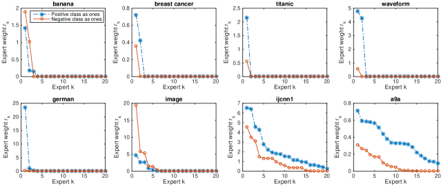
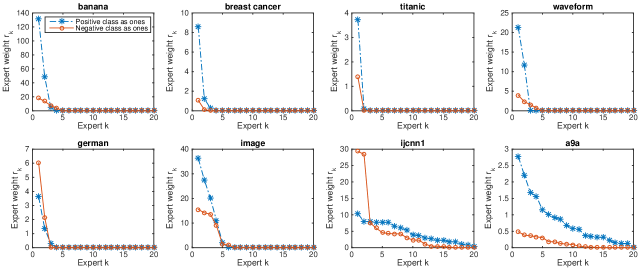
Figure 9: The inferred weights of the $K_{\max}=20$ experts of sum-softplus regression, ordered from left to right according to their weights, on all datasets shown in Tab. 6, based on the maximum likelihood sample of a single random trial.

Figure 10: Analogous to Fig. 10 for SS-softplus regression with $K_{\max}=20$ and $T=5$.

For both stack- and SS-softplus regressions, the computational complexity in both training and out-of-sample prediction increases linearly in $T$, the depth of the stack. To understand how increasing $T$ affects the performance, we show in Tabs. 6-6 of Appendix E the classification errors of stack- and SS-softplus regressions, respectively, for $T\in\{1,2,3,5,10\}$. It is clear that increasing $T$ from 1 to 2 generally leads to the most significant improvement if there is a clear advantage of increasing $T$, and once $T$ is sufficiently large, further increasing $T$ leads to small fluctuations of the performance but does not appear to lead to clear overfitting. It is also interesting to examine the number of active experts inferred by SS-softplus regression, where each expert is equipped with $T$ hyperplanes, as $T$ increases. As shown in Tab. 6 of Appendix E, this number has a clear increasing trend as $T$ increases. This is not surprising as each expert is able to fit more complex geometric structure as $T$ increases, and hence SS-softplus regression can employ more of them to more detailedly describe the decision boundaries. This phenomenon is also clearly visualized in comparing the inferred experts and decision boundaries for SS-softplus regression, as shown in Fig. 6, with those for sum-softplus regression, as shown in Fig. 1.

In addition to comparing softplus regressions with related algorithms on the six benchmark datasets used in Tipping (2001), we also consider ijcnn1 and a9a, two larger-scale benchmark datasets that have also been used in Chang et al. (2010); Wang et al. (2011) and Kantchelian et al. (2014). In Appendix E, we report results on both datasets, whose training/testing partition is predefined, based on a single random trial for logistic regression, SVM, and RVM, and five independent random trials for AMM, CPM, and all softplus regressions. As shown in Tabs. 10-10 of Appendix E, we observe similar relationships between the classification errors and the number of expert criteria for both stack- and SS-softplus regressions, and both sum- and SS-softplus regressions provide a good comprise between the classification accuracies and amount of computation required for out-of-sample predictions.

As shown in Figs. 10-10, with the upper-bound of the number of experts set as $K_{\max}=20$, for each of the first six datasets, both sum- and SS-softplus regressions shrink the weights of most of the 20 experts to be close to zero, clearly inferring the number of experts with non-negligible weights under both labeling settings. For both ijcnn1 and a9a, at one of the two labeling setting for both sum- and SS-softplus regressions, $K_{\max}=20$ does not seem to be large enough to accommodate all experts with non-negligible weights. Thus we have also tried setting $K_{\max}=50$, which is found to more clearly show the ability of the model to shrink the weights of unnecessary experts for both ijcnn1 and a9a, but at the expense of clearly increased computational complexity in both training and testing. The automatic shrinkage mechanism of the gamma process based sum- and SS-softplus regressions is attractive for both computation and implementation, as it allows setting $K_{\max}$ as large as permitted by the computational budget, without the need to worry about overfitting. Having the ability to support countably infinite experts in the prior and inferring a finite number of experts with non-negligible weights in the posterior is an attractive property of the proposed nonparametric Bayesian softplus regression models.

We comment that while we choose a fixed truncation to approximate a countably infinite nonparametric Bayesian model, it is possible to adaptive truncate the number of experts for the proposed gamma process based models, using strategies such as marginalizing out the underlying stochastic processes (Teh et al., 2006; Lijoi et al., 2007), performing reversible-jump MCMC (Green, 1995; Wolpert et al., 2011), and using slice sampling (Walker, 2007; Neal, 2003), which would be interesting topics for future research.

5 Conclusions

To regress a binary response variable on its covariates, we propose sum-, stack-, and sum-stack-softplus regressions that use, respectively, a convex-polytope-bounded confined space to enclose the negative class, a convex-polytope-like confined space to enclose the positive class, and a union of convex-polytope-like confined spaces to enclose the positive class. Sum-stack-softplus regression, including logistic regression and all the other softplus regressions as special examples, constructs a highly flexible nonparametric Bayesian predictive distribution by mixing the convolved and stacked covariate-dependent gamma distributions with the Bernoulli-Poisson distribution. The predictive distribution is deconvolved and demixed by inferring the parameters of the underlying nonparametric Bayesian hierarchical model using a series of data augmentation and marginalization techniques. In the proposed Gibbs sampler that has closed-form update equations, the parameters of different stacked gamma distributions can be updated in parallel within each iteration. Example results demonstrate that the proposed softplus regressions can achieve classification accuracies comparable to those of kernel support vector machine, but consume significant less computation for out-of-sample predictions, provide probability estimates, quantify uncertainties, and place interpretable geometric constraints on its classification decision boundaries directly in the original covariate space. It is of great interest to investigate how to generalize the proposed softplus regressions to model count, categorical, ordinal, and continuous response variables, and to model observed or latent multivariate discrete vectors. For example, to introduce covariate-dependence into a stick-breaking process mixture model (Ishwaran and James, 2001), one may consider replacing the normal cumulative distribution function used in the probit stick-breaking process of Chung and Dunson (2009) or the logistic function used in the logistic stick-breaking process of Ren et al. (2011) with the proposed softplus functions.

Appendix A Polya-Gamma distribution

To infer the regression coefficient vector for each NB regression, we use the Polya-Gamma random variable $X\sim\mbox{PG}(a,c)$, defined in Polson and Scott (2011) as the weighted sum of infinite independent, and identically distributed ($i.i.d.$) gamma random variables as

$$X=\frac{1}{2\pi^{2}}\sum_{k=1}^{\infty}\frac{g_{k}}{(k-1/2)^{2}+c^{2}/(4\pi^{2})},~{}~{}g_{k}\sim\mbox{Gamma}(a,1).\vspace{0mm}$$ (29)

As in Polson et al. (2013), the moment generating function of the Polya-Gamma random variable $X\sim\mbox{PG}(a,c)$ can be expressed as

$$\mathbb{E}[e^{sX}]={\cosh^{a}\left(\frac{c}{2}\right)}{\cosh^{-a}\left(\sqrt{\frac{c^{2}/2-s}{2}}\right)}.\vspace{0mm}$$

Let us denote $f(s)=\sqrt{\frac{c^{2}/2-s}{2}}$ and hence $f^{\prime}(s)=-1/[4f(s)]$. Since

$$\frac{d\mathbb{E}[e^{sX}]}{ds}=\frac{a}{4}\mathbb{E}[e^{sX}]\frac{\tanh[f(s)]}{f(s)},$$

$$\frac{d^{2}\mathbb{E}[e^{sX}]}{ds^{2}}=\frac{1}{\mathbb{E}[e^{sX}]}\left(\frac{d\mathbb{E}[e^{sX}]}{ds}\right)^{2}+\frac{a}{4}\mathbb{E}[e^{sX}]\cosh^{-2}[f(s)]\frac{\sinh[2f(s)]-2f[s]}{[2f(s)]^{3}},$$

the mean can be expressed as

$$\mathbb{E}[X\,|\,a,c]=\frac{d\mathbb{E}[e^{sX}]}{ds}(0)=\frac{a}{2|c|}\tanh\left(\frac{|c|}{2}\right),\vspace{0mm}$$ (30)

and the variance can be expressed as

$$\mbox{var}[X\,|\,a,c] =\frac{d^{2}\mathbb{E}[e^{sX}]}{ds^{2}}(0)-(\mathbb{E}[X])^{2}=\frac{a\cosh^{-2}\big{(}{|c|}/{2}\big{)}{[\sinh(|c|)-|c|]}}{4|c|^{3}}=\frac{a}{2|c|^{3}}\frac{{\sinh(|c|)-|c|}}{\cosh(|c|)+1}$$

$$=\frac{a}{2|c|^{3}}\frac{1-e^{-2|c|}-2|c|e^{-|c|}}{1+e^{-2|c|}+2e^{-|c|}}=\frac{a\cosh^{-2}\left(\frac{|c|}{2}\right)}{4}\left(\frac{1}{6}+\sum_{n=1}^{\infty}\frac{|c|^{2n}}{(2n+3)!}\right),$$ (31)

which matches the variance shown in Glynn et al. (2015) but with a much simpler derivation.

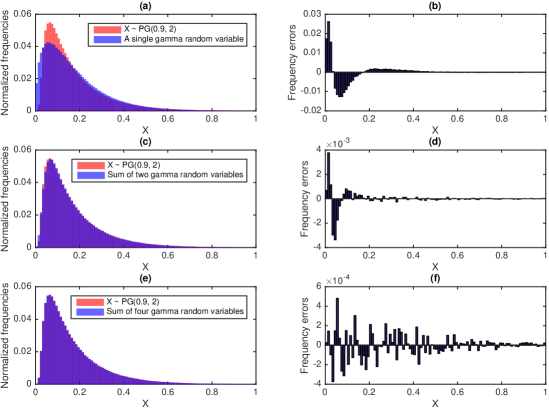
Figure 11: (a) Comparison of the normalized histogram of $10^{6}$ independent random samples following $X\sim\mbox{PG}(0.9,2)$ (simulated using the truncated sampler at a truncation level of 1000) and that of $10^{6}$ ones simulated with the approximate sampler truncated at one, $i.e.$, simulated from $X\sim\mbox{Gamma}\left({\mu_{\triangle}^{2}}/{\sigma^{2}_{\triangle}},{\sigma^{2}_{\triangle}}/{\mu_{\triangle}}\right)$, where $\mu_{\triangle}=0.1714$ and $\sigma^{2}_{\triangle}=0.0192$ are chosen to match the mean and variance of $X\sim\mbox{PG}(0.9,2)$; (b) the differences between the normalized frequencies of these two histograms. (c)-(d): analogous plots to (a)-(b), with the truncated sampler truncated at two. (e)-(f): analogous plots to (a)-(b), with the truncated sampler truncated at four.

As in (29), a PG distributed random variable can be generated from an infinite sum of weighted $i.i.d.$ gamma random variables. In Polson et al. (2013), when $a$ is an integer, $X\sim\mbox{PG}(a,c)$ is sampled exactly using a rejection sampler, but when $a$ is a positive real number, it is sampled approximately by truncating the infinite sum in (29). However, the mean of $X$ approximately generated in this manner is guaranteed to be left biased. An improved approximate sampler is proposed in Zhou et al. (2012b) to compensate the bias of the mean, but not the bias of the variance.

We present in Proposition 10 an approximate sampler that is unbiased in both the mean and variance, using the summation of a finite number of gamma random variables. As shown in Fig. 11, the approximate sampler is quite accurate even only using two gamma random variables. We also provide some additional propositions, whose proofs are deferred to Appendix B, to describe some important properties that will be used in inference.

Proposition 10.

Denoting $K\in\{1,2,\ldots\}$ as a truncation level, if

$$\hat{X}=\frac{1}{2\pi^{2}}\sum_{k=1}^{K-1}\frac{g_{k}}{(k-1/2)^{2}+c^{2}/(4\pi^{2})},~{}~{}g_{k}\sim\emph{\mbox{Gamma}}(a,1)\vspace{0mm}$$ (32)

and $X_{\triangle}\sim\emph{\mbox{Gamma}}\left({\mu_{\triangle}^{2}}{\sigma^{-2}_{\triangle}},{\mu^{-1}_{\triangle}}{\sigma^{2}_{\triangle}}\right),$ where

$$\displaystyle\mu_{\triangle}=\frac{a}{2|c|}\tanh\left(\frac{|c|}{2}\right)-\mathbb{E}[\hat{X}],~{}~{}~{}\displaystyle\sigma^{2}_{\triangle}=\frac{a}{2|c|^{3}}\frac{{\sinh(|c|)-|c|}}{\cosh(|c|)+1}-\emph{\mbox{var}}[\hat{X}],\vspace{0mm}$$

then $\hat{X}+X_{\triangle}$ has the same mean and variance as those of $X\sim\emph{\mbox{PG}}(a,c)$, and the difference between their cumulant generating functions can be expressed as

$$\ln\mathbb{E}[e^{sX}]-\ln\mathbb{E}[e^{s(\hat{X}+X_{\triangle})}]=\sum_{n=3}^{\infty}\frac{s^{n}}{n}\left[\left(a\sum_{k=K}^{\infty}d_{k}^{-n}\right)-\frac{\mu_{\triangle}^{2}}{\sigma^{2}_{\triangle}}\left(\frac{\sigma^{2}_{\triangle}}{\mu_{\triangle}}\right)^{n}\right],\vspace{0mm}$$

where $d_{k}=2\pi^{2}(k-1/2)^{2}+c^{2}/2.$

Proposition 11.

If $X\sim\emph{\mbox{PG}}(a,c)$, then $\lim_{|c|\rightarrow\infty}X=0$ and $\lim_{|c|\rightarrow\infty}|c|X=a/2$.

Proposition 12.

If $X\sim\emph{\mbox{PG}}(a,0)$, then $\mathbb{E}[X\,|\,a,0]=a/4$ and $\emph{\mbox{var}}[X\,|\,a,0]=a/24$.

Proposition 13.

If $X\sim\emph{\mbox{PG}}(a,c)$, then $\displaystyle\emph{\mbox{var}}[X\,|\,a,c]\geq\frac{a}{24}{\cosh^{-2}\left(\frac{|c|}{2}\right)}$, where the equality holds if and only if $c=0$.

Proposition 14.

$X\sim\emph{\mbox{PG}}(a,c)$ has a variance-to-mean ratio as

$$\frac{\emph{\mbox{var}}[X\,|\,a,c]}{\mathbb{E}[X\,|\,a,c]}=\frac{1}{|c|^{2}}-\frac{1}{|c|\sinh(|c|)}$$

and is always under-dispersed, since $\emph{\mbox{var}}[X\,|\,a,c]\leq\mathbb{E}[X\,|\,a,c]/6$ almost surely, where the equality holds if and only if $c=0$.

Appendix B Proofs

Proof for Definition 1.

For the hierarchical model in (7), we have $P(y_{i}=0\,|\,\theta_{i})=e^{-\theta_{i}}$. Further using the moment generating function of the gamma distribution, we have

$$P(y_{i}=0\,|\,\boldsymbol{x}_{i},{\boldsymbol{\beta}})=\mathbb{E}_{\theta_{i}}[e^{-\theta_{i}}]=(1+e^{\boldsymbol{x}_{i}^{\prime}{\boldsymbol{\beta}}})^{-1}.\vspace{0mm}$$

As $\lambda(\boldsymbol{x}_{i})=-\ln[P(y_{i}=0\,|\,\boldsymbol{x}_{i},{\boldsymbol{\beta}})]$ by definition, we have $\lambda(\boldsymbol{x}_{i})=\ln(1+e^{\boldsymbol{x}_{i}^{\prime}{\boldsymbol{\beta}}})$. ∎

Proof for Definition 2.

For the hierarchical model in (9), we have $P(y_{i}=0\,|\,\theta_{i})=e^{-\theta_{i}}=\prod_{k=1}^{\infty}e^{-\theta_{ik}}$. Using the moment generating function of the gamma distribution, we have

$$P(y_{i}=0\,|\,\boldsymbol{x}_{i},\{{\boldsymbol{\beta}}_{k}\}_{k})=\mathbb{E}_{\theta_{i}}\left[\prod_{k=1}^{\infty}e^{-\theta_{ik}}\right]=\prod_{k=1}^{\infty}\mathbb{E}_{\theta_{ik}}[e^{-\theta_{ik}}]=\prod_{k=1}^{\infty}(1+e^{\boldsymbol{x}_{i}^{\prime}{\boldsymbol{\beta}}_{k}})^{-r_{k}}.\vspace{0mm}$$

As $\lambda(\boldsymbol{x}_{i})=-\ln[P(y_{i}=0\,|\,\boldsymbol{x}_{i},\{{\boldsymbol{\beta}}_{k}\}_{k})]$ by definition, we obtain (8). ∎

Proof for Definition 3.

For the hierarchical model in (11), we have $P(y_{i}=0\,|\,\theta^{(1)}_{i})=e^{-\theta_{i}^{(1)}}$. Using the moment generating function of the gamma distribution, we have

$$P(y_{i}=0\,|\,\boldsymbol{x}_{i},{\boldsymbol{\beta}}^{(2)},\theta_{i}^{(2)})=\mathbb{E}_{\theta_{i}^{(1)}}\left[e^{-\theta_{i}^{(1)}}\right]=(1+e^{\boldsymbol{x}_{i}^{\prime}{\boldsymbol{\beta}}^{(2)}})^{-\theta_{i}^{(2)}}=e^{-\theta_{i}^{(2)}\ln(1+e^{\boldsymbol{x}_{i}^{\prime}{\boldsymbol{\beta}}^{(2)}})}.\vspace{0mm}$$

Marginalizing out $\theta_{i}^{(2)}$ leads to

$$P(y_{i}=0\,|\,\boldsymbol{x}_{i},{\boldsymbol{\beta}}^{(2:3)},\theta_{i}^{(3)})=\mathbb{E}_{\theta_{i}^{(2)}}\left[e^{-\theta_{i}^{(2)}\ln(1+e^{\boldsymbol{x}_{i}^{\prime}{\boldsymbol{\beta}}^{(2)}})}\right]=e^{-\theta_{i}^{(3)}\ln[1+e^{\boldsymbol{x}_{i}^{\prime}{\boldsymbol{\beta}}^{(3)}}\ln(1+e^{\boldsymbol{x}_{i}^{\prime}{\boldsymbol{\beta}}^{(2)}})]}.\vspace{0mm}$$

Further marginalizing out $\theta_{i}^{(3)},\ldots,\theta_{i}^{(T)}$ and with $\lambda(\boldsymbol{x}_{i})=-\ln[P(y_{i}=0\,|\,\boldsymbol{x}_{i},r,{\boldsymbol{\beta}}^{(2:T+1)})]$ by definition, we obtain (10). ∎

Proof for Definition 4.

For the hierarchical model in (13), we have $P(y_{i}=0\,|\,\{\theta^{(1)}_{ik}\}_{k})=e^{-\sum_{k=1}^{\infty}\theta_{ik}^{(1)}}$. Using the moment generating function of the gamma distribution, we have

$$P(y_{i}=0\,|\,\boldsymbol{x}_{i},\{{\boldsymbol{\beta}}_{k}^{(2)},\theta_{ik}^{(2)}\}_{k})=\prod_{k=1}^{\infty}e^{-\theta_{ik}^{(2)}\ln\big{(}1+e^{\boldsymbol{x}_{i}^{\prime}{\boldsymbol{\beta}}_{k}^{(2)}}\big{)}}.\vspace{0mm}$$

Further marginalizing out $\{\theta_{ik}^{(2)}\}_{k},\ldots,\{\theta_{ik}^{({T})}\}_{k}$ and by definition with $\lambda(\boldsymbol{x}_{i})=-\ln[P(y_{i}=0\,|\,\boldsymbol{x}_{i},\{r_{k},{\boldsymbol{\beta}}_{k}^{(2:{T}+1)}\}_{k})]$, we obtain (12). ∎

Proof of Proposition 1.

By construction, the infinite product would be equal or small than one. We need to further make sure that the infinite product would not degenerate to zero. Using the Lévy-Khintchine theorem (Kallenberg, 2006), we have

$$-\ln\left\{\mathbb{E}_{G}\left[e^{{-\sum_{k=1}^{\infty}r_{k}\ln[1+\exp(\boldsymbol{x}_{i}^{\prime}{\boldsymbol{\beta}}_{k})]}}\right]\right\} =\int_{\mathbb{R}_{+}\times\Omega}\left[1-\left(\frac{1}{1+e^{\boldsymbol{x}_{i}^{\prime}{\boldsymbol{\beta}}}}\right)^{r}\right]\nu(drd{\boldsymbol{\beta}}).$$

where $\nu(drd{\boldsymbol{\beta}})=r^{-1}e^{-cr}drG_{0}(d{\boldsymbol{\beta}})$ is the Lévy measure of the gamma process. Since if $c\geq 0$, then $1-e^{-cx}\leq cx$ for all $x\geq 0$, the right-hand-side term of the above equation would be bounded below

$$\int_{\mathbb{R}_{+}\times\Omega}r\ln[1+e^{\boldsymbol{x}_{i}^{\prime}{\boldsymbol{\beta}}}]\nu(drd{\boldsymbol{\beta}})=\frac{\gamma_{0}}{c}\int_{\Omega}\ln[1+e^{\boldsymbol{x}_{i}^{\prime}{\boldsymbol{\beta}}}]g_{0}(d{\boldsymbol{\beta}}).$$ (33)

Since $e^{e^{x}}=1+e^{x}+\sum_{n=2}^{\infty}\frac{e^{nx}}{n!}\geq 1+e^{x},$ we have

$$\ln(1+e^{x})\leq e^{x},\vspace{0mm}$$ (34)

where the equality is true if and only if $x=-\infty$. Assuming ${\boldsymbol{\beta}}\sim\mathcal{N}(0,{\boldsymbol{\Sigma}})$, we have

$$\int_{\Omega}\ln[1+e^{\boldsymbol{x}_{i}^{\prime}{\boldsymbol{\beta}}}]g_{0}(d{\boldsymbol{\beta}})\leq\int_{\Omega}e^{\boldsymbol{x}^{\prime}_{i}{\boldsymbol{\beta}}}\mathcal{N}({\boldsymbol{\beta}};0,{\boldsymbol{\Sigma}})d{\boldsymbol{\beta}}=e^{\frac{1}{2}\boldsymbol{x}_{i}^{\prime}{\boldsymbol{\Sigma}}\boldsymbol{x}_{i}}\vspace{0mm}$$

Thus the integral in the right-hand-side of (33) is finite and hence the infinite product $\prod_{k=1}^{\infty}\left[{1+e^{\boldsymbol{x}_{i}^{\prime}{\boldsymbol{\beta}}_{k}}}\right]^{-r_{k}}$ has a finite expectation that is greater than zero. ∎

Proof of Theorem 2.

Since $\sum_{k^{\prime}\neq k}r_{k^{\prime}}\ln(1+e^{\boldsymbol{x}_{i}^{\prime}{\boldsymbol{\beta}}_{k^{\prime}}})\geq 0$ a.s., if (16) is true, then $r_{k}\ln(1+e^{\boldsymbol{x}_{i}^{\prime}{\boldsymbol{\beta}}_{k}})\leq-\ln(1-p_{0})$ a.s. for all $k\in\{1,2,\ldots\}$. Thus if (16) is true, then (17) is true a.s., which means the set of solutions to (16) is included in the set of solutions to (17). ∎

Proof of Proposition 3.

Assuming $\boldsymbol{x}_{i}$ violates at least the $k$th inequality, which means $\boldsymbol{x}_{i}^{\prime}{\boldsymbol{\beta}}_{k}>\ln\big{[}(1-p_{0})^{-\frac{1}{r_{k}}}-1\big{]},$ then we have

$$\lambda(\boldsymbol{x}_{i})=r_{k}\ln(1+e^{\boldsymbol{x}_{i}^{\prime}{\boldsymbol{\beta}}_{k}})+\sum_{k^{\prime}\neq k}r_{k^{\prime}}\ln(1+e^{\boldsymbol{x}_{i}^{\prime}{\boldsymbol{\beta}}_{k^{\prime}}})\geq r_{k}\ln(1+e^{\boldsymbol{x}_{i}^{\prime}{\boldsymbol{\beta}}_{k}})>-\ln(1-p_{0})$$

and hence $P(y_{i}=1\,|\,\boldsymbol{x}_{i})=1-e^{-\lambda(\boldsymbol{x}_{i})}>p_{0}$ and $P(y_{i}=0\,|\,\boldsymbol{x}_{i})\leq 1-p_{0}$. ∎

Proof of Proposition 4.

By construction, the infinite product would be equal or small than one. We need to further make sure that the infinite product would not degenerate to zero. Using the Lévy-Khintchine theorem (Kallenberg, 2006) and $1-e^{-cx}\leq cx$ for all $x\geq 0$ if $c\geq 0$, we have

$$-\ln\left\{\mathbb{E}_{G}\exp\left[{-\sum_{k=1}^{\infty}r_{k}\ln\left(1+e^{\boldsymbol{x}_{i}^{\prime}{\boldsymbol{\beta}}^{({T}+1)}_{k}}\ln\Bigg{\{}1+e^{\boldsymbol{x}_{i}^{\prime}{\boldsymbol{\beta}}^{({T})}_{k}}\ln\bigg{[}1+\ldots\ln\Big{(}1+e^{\boldsymbol{x}_{i}^{\prime}{\boldsymbol{\beta}}^{(2)}_{k}}\Big{)}\bigg{]}\Bigg{\}}\right)}\right]\right\}$$

$$=\int\left[1-\left(1+e^{\boldsymbol{x}_{i}^{\prime}{\boldsymbol{\beta}}^{({T}+1)}}\ln\Bigg{\{}1+e^{\boldsymbol{x}_{i}^{\prime}{\boldsymbol{\beta}}^{({T})}}\ln\bigg{[}1+\ldots e^{\boldsymbol{x}_{i}^{\prime}{\boldsymbol{\beta}}^{(3)}}\ln\Big{(}1+e^{\boldsymbol{x}_{i}^{\prime}{\boldsymbol{\beta}}^{(2)}}\Big{)}\bigg{]}\Bigg{\}}\right)^{-r}\right]\nu(drd{\boldsymbol{\beta}}^{({T}+1:2)})$$

$$\leq\int r\ln\left(1+e^{\boldsymbol{x}_{i}^{\prime}{\boldsymbol{\beta}}^{({T}+1)}}\ln\Bigg{\{}1+e^{\boldsymbol{x}_{i}^{\prime}{\boldsymbol{\beta}}^{({T})}}\ln\bigg{[}1+\ldots e^{\boldsymbol{x}_{i}^{\prime}{\boldsymbol{\beta}}^{(3)}}\ln\Big{(}1+e^{\boldsymbol{x}_{i}^{\prime}{\boldsymbol{\beta}}^{(2)}}\Big{)}\bigg{]}\Bigg{\}}\right)\nu(drd{\boldsymbol{\beta}}^{({T}+1:2)}).$$ (35)

Since $\ln(1+e^{x})\leq e^{x},$ we have

$$\ln\left(1+e^{\boldsymbol{x}_{i}^{\prime}{\boldsymbol{\beta}}^{({T}+1)}}\ln\Bigg{\{}1+e^{\boldsymbol{x}_{i}^{\prime}{\boldsymbol{\beta}}^{({T})}}\ln\bigg{[}1+\ldots e^{\boldsymbol{x}_{i}^{\prime}{\boldsymbol{\beta}}^{(3)}}\ln\Big{(}1+e^{\boldsymbol{x}_{i}^{\prime}{\boldsymbol{\beta}}^{(2)}}\Big{)}\bigg{]}\Bigg{\}}\right)$$

$$\leq~{} \ln\left(1+e^{\boldsymbol{x}_{i}^{\prime}{\boldsymbol{\beta}}^{({T}+1)}}\ln\Bigg{\{}1+e^{\boldsymbol{x}_{i}^{\prime}{\boldsymbol{\beta}}^{({T})}}\ln\bigg{[}1+\ldots e^{\boldsymbol{x}_{i}^{\prime}{\boldsymbol{\beta}}^{(4)}}\ln\Big{(}1+e^{\boldsymbol{x}_{i}^{\prime}({\boldsymbol{\beta}}^{(3)}+{\boldsymbol{\beta}}^{(2)})}\Big{)}\bigg{]}\Bigg{\}}\right)$$

$$\leq~{} \ln\left(1+e^{\boldsymbol{x}_{i}^{\prime}{\boldsymbol{\beta}}^{(\star)}}\right)\leq e^{\boldsymbol{x}_{i}^{\prime}{\boldsymbol{\beta}}^{(\star)}}$$

where ${\boldsymbol{\beta}}^{(\star)}:={\boldsymbol{\beta}}^{({T}+1)}+{\boldsymbol{\beta}}^{({T})}+\ldots+{\boldsymbol{\beta}}^{(2)}$. Assuming ${\boldsymbol{\beta}}^{(t)}\sim\mathcal{N}(0,{\boldsymbol{\Sigma}}_{t})$, the right hand side of (35) would be bound below $\int re^{\boldsymbol{x}_{i}^{\prime}{\boldsymbol{\beta}}^{(\star)}}\nu(drd{\boldsymbol{\beta}}^{(\star)})=\gamma_{0}c^{-1}e^{\frac{1}{2}\boldsymbol{x}_{i}^{\prime}(\sum_{t=2}^{T+1}{\boldsymbol{\Sigma}}_{t})\boldsymbol{x}_{i}}.$ Therefore, the integral in the right-hand-side of (35) is finite and hence the infinite product in Proposition 4 has a finite expectation that is greater than zero under the gamma process. ∎

Proof of Theorem 5.

Since

$$\sum_{k^{\prime}\neq k}r_{k^{\prime}}\ln\left(1+e^{\boldsymbol{x}_{i}^{\prime}{\boldsymbol{\beta}}^{({T}+1)}_{k^{\prime}}}\ln\Bigg{\{}1+e^{\boldsymbol{x}_{i}^{\prime}{\boldsymbol{\beta}}^{({T})}_{k^{\prime}}}\ln\bigg{[}1+\ldots\ln\Big{(}1+e^{\boldsymbol{x}_{i}^{\prime}{\boldsymbol{\beta}}^{(2)}_{k^{\prime}}}\Big{)}\bigg{]}\Bigg{\}}\right)\geq 0$$

a.s., if (23) is true for at least one $k\in\{1,2,\ldots\}$, then (22) is true a.s., which means the set of solutions to $\eqref{eq:SS-softplus_ineuqality}$ encompass $\mathcal{D}_{\star}$. ∎

Proof of Proposition 7.

Assume $\boldsymbol{x}_{i}$ satisfies at least the $k$th inequality, which means (23) is true, then

$$\small\lambda(\boldsymbol{x}_{i})\geq r_{k}\ln\left(1+e^{\boldsymbol{x}_{i}^{\prime}{\boldsymbol{\beta}}^{({T}+1)}_{k}}\ln\Bigg{\{}1+e^{\boldsymbol{x}_{i}^{\prime}{\boldsymbol{\beta}}^{({T})}_{k}}\ln\bigg{[}1+\ldots\ln\Big{(}1+e^{\boldsymbol{x}_{i}^{\prime}{\boldsymbol{\beta}}^{(2)}_{k}}\Big{)}\bigg{]}\Bigg{\}}\right)>-\ln(1-p_{0})$$

and hence $P(y_{i}=1\,|\,\boldsymbol{x}_{i})=1-e^{-\lambda(\boldsymbol{x}_{i})}>p$ and $P(y_{i}=0\,|\,\boldsymbol{x}_{i})\leq 1-p_{0}$. ∎

Proof of Theorem 8.

By construction (27) is true for $t=1$. Suppose (27) is also true for $t\geq 2$, then we can augment each $m_{ik}^{(t)}$ under its compound Poisson representation as

$$m_{ik}^{(t)}\,|\,m_{ik}^{(t+1)}\sim\mbox{SumLog}(m_{ik}^{(t+1)},~{}p_{ik}^{(t+1)}),~{}~{}m_{ik}^{(t+1)}\sim\mbox{Pois}\left(\theta_{ik}^{(t+1)}q_{ik}^{(t+1)}\right),\vspace{0mm}$$ (36)

where the joint distribution of $m_{ik}^{(t)}$ and $m_{ik}^{(t+1)}$, according to Theorem 1 of Zhou and Carin (2015), is the same as that in

$$m_{ik}^{(t+1)}\,|\,m_{ik}^{(t)}\sim\mbox{CRT}(m_{ik}^{(t)},~{}\theta_{ik}^{(t+1)}),~{}~{}m_{ik}^{(t)}\sim{\mbox{NB}}(\theta_{ik}^{(t+1)},~{}p_{ik}^{(t+1)}),\vspace{0mm}$$

where CRT refers to the Chinese restaurant table distribution described in Zhou and Carin (2015). Marginalizing $\theta_{ik}^{(t+1)}$ from the Poisson distribution in (36) leads to $m_{ik}^{(t+1)}\sim{\mbox{NB}}(\theta_{ik}^{(t+2)},$ $p_{ik}^{(t+2)})$. Thus if (27) is true for layer $t$, then it is also true for layer $t+1$. ∎

Proof of Proposition 10.

Since $\hat{X}$ and $X_{\triangle}$ are independent to each other, with (30) and (A), we have and $\mathbb{E}[X]=\mathbb{E}[\hat{X}]+\mu_{\triangle}=\mathbb{E}[\hat{X}+X_{\triangle}]$ and $\mbox{var}[X]=\mbox{var}[\hat{X}]+\sigma^{2}_{\triangle}=\mbox{var}[\hat{X}+X_{\triangle}]$. Using Taylor series expansion, we have

$$\ln\mathbb{E}[e^{sX}] =-\sum_{k=1}^{\infty}a\ln(1-sd_{k}^{-1})=a\sum_{k=1}^{\infty}\sum_{n=1}^{\infty}\frac{s^{n}d_{k}^{-n}}{n}=s\mathbb{E}[X]+s^{2}\frac{\mbox{var}[X]}{2}+a\sum_{n=3}^{\infty}\sum_{k=1}^{\infty}\frac{s^{n}d_{k}^{-n}}{n},$$

$$\ln\mathbb{E}[e^{s\hat{X}}] =-\sum_{k=1}^{K-1}a\ln(1-sd_{k}^{-1})=s\mathbb{E}[\hat{X}]+s^{2}\frac{\mbox{var}[\hat{X}]}{2}+a\sum_{n=3}^{\infty}\sum_{k=1}^{K-1}\frac{s^{n}d_{k}^{-n}}{n},$$

$$\ln\mathbb{E}[e^{sX_{\triangle}}] =-\frac{\mu_{\triangle}^{2}}{\sigma^{2}_{\triangle}}\ln\left(1-s\frac{\sigma^{2}_{\triangle}}{\mu_{\triangle}}\right)=\frac{\mu_{\triangle}^{2}}{\sigma^{2}_{\triangle}}\sum_{n=1}^{\infty}\frac{s^{n}(\frac{\sigma^{2}_{\triangle}}{\mu_{\triangle}})^{n}}{n}=s\mu_{\triangle}+s^{2}\frac{\sigma^{2}_{\triangle}}{2}+\frac{\mu_{\triangle}^{2}}{\sigma^{2}_{\triangle}}\sum_{n=3}^{\infty}\frac{s^{n}(\frac{\sigma^{2}_{\triangle}}{\mu_{\triangle}})^{n}}{n}.$$

The proof is completed with $\ln\mathbb{E}[e^{sX}]-\ln\mathbb{E}[e^{s(\hat{X}+X_{\triangle})}]=\ln\mathbb{E}[e^{sX}]-\ln\mathbb{E}[e^{s(\hat{X})}]-\ln\mathbb{E}[e^{X_{\triangle})}].$ ∎

Proof of Proposition 11.

For the Polya-Gamma random variable $X\sim\mbox{PG}(a,c)$, since $\mathbb{E}[X]=\frac{a}{2|c|}\tanh\big{(}\frac{|c|}{2}\big{)}$ and $\lim_{|c|\rightarrow\infty}\tanh\big{(}\frac{|c|}{2}\big{)}=1$, we have $\lim_{|c|\rightarrow\infty}\mathbb{E}[X]=0$. With the expression of $\mbox{var}[X]$ shown in (A), we have $\lim_{|c|\rightarrow\infty}\mbox{var}[X]=0$. Therefore, we have $X\rightarrow 0$ as $|c|\rightarrow\infty$.

Since $\lim_{|c|\rightarrow\infty}\mathbb{E}[|c|X]=a/2$ and

$$\mbox{var}[|c|X]=(|c|)^{2}\mbox{var}[X]=\frac{a}{2|c|}\frac{{\sinh(|c|)-|c|}}{\cosh(|c|)+1}=\frac{a}{2}\frac{{\frac{\tanh(|c|)}{|c|}-\cosh^{-1}(|c|)}}{1+\cosh^{-1}(|c|)}.$$

we have $\lim_{|c|\rightarrow\infty}\mbox{var}[|c|X]=0$ and hence $\lim_{|c|\rightarrow\infty}|c|X=a/2$. ∎

Proof of Proposition 12.

Using (30), we have

$$\mathbb{E}[X\,|\,a,0]=\lim_{c\rightarrow 0}\mathbb{E}[X\,|\,a,c]=\lim_{c\rightarrow 0}\frac{a}{2|c|}\tanh\left(\frac{|c|}{2}\right)=\lim_{c\rightarrow 0}\frac{a}{2}\frac{e^{|c|}-1}{|c|}\frac{1}{e^{|c|}+1}=\frac{a}{4}.\vspace{0mm}$$

Using (A), we have
$\displaystyle~{}~{}~{}~{}~{}~{}~{}\mbox{var}[X\,|\,a,0]=\lim_{c\rightarrow 0}\mbox{var}[X\,|\,a,c]=\lim_{c\rightarrow 0}\frac{a\cosh^{-2}\left(\frac{|c|}{2}\right)}{4}\left(\frac{1}{6}+\sum_{n=1}^{\infty}\frac{|c|^{2n}}{(2n+3)!}\right)=\frac{a}{24}.$ ∎

Proof of Proposition 13.

Using (A), we have $\mbox{var}[X\,|\,a,c]=\frac{a\cosh^{-2}\left(\frac{|c|}{2}\right)}{4}\left(\frac{1}{6}+\sum_{n=1}^{\infty}\frac{|c|^{2n}}{(2n+3)!}\right)\geq\frac{a}{24}\cosh^{-2}\left(\frac{|c|}{2}\right)$, with the equality holds if and only if $c=0$. ∎

Proof of Proposition 14.

With (30) and (A), the variance-to-mean ratio is

$$\small\frac{\mbox{var}[X\,|\,a,c]}{\mathbb{E}[X\,|\,a,c]}=\frac{1}{|c|^{2}}-\frac{1}{|c|\sinh(|c|)}=\frac{\sinh(|c|)-|c|}{|c|^{2}\sinh(|c|)}=\left[{\frac{1}{6}\displaystyle\sum_{n=0}^{\infty}\frac{|c|^{2n+3}\,3!}{(2n+3)!}}\right]\left/\left[{\displaystyle\sum_{n=0}^{\infty}\frac{|c|^{2n+3}}{(2n+1)!}}\right]\right..\vspace{0mm}$$

When $c=0$, with Proposition 12, we have ${\mbox{var}[X\,|\,a,c]}\big{/}{\mathbb{E}[X\,|\,a,c]}=1/6$. When $c\neq 0$, since $3!/(2n+3)!<1/(2n+1)!$ a.s. for all $n\in\{1,\ldots\}$, we have

$$\sum_{n=0}^{\infty}\frac{|c|^{2n+3}\,3!}{(2n+3)!}<\sum_{n=0}^{\infty}\frac{|c|^{2n+3}}{(2n+1)!}$$

a.s. and hence ${\mbox{var}[X\,|\,a,c]}\big{/}{\mathbb{E}[X\,|\,a,c]}<1/6$ a.s. ∎

Appendix C Gibbs sampling for sum-stack-softplus regression

For SS-softplus regression, Gibbs sampling via data augmentation and marginalization proceeds as follows.
Sample $m_{i}$. Denote $\theta_{i\boldsymbol{\cdot}}=\sum_{k=1}^{K}\theta^{(1)}_{ik}$ . Since $m_{i}=0$ a.s. given $y_{i}=0$ and $m_{i}\geq 1$ given $y_{i}=1$, and in the prior we have $m_{i}\sim\mbox{Pois}(\theta_{i\boldsymbol{\cdot}})$, following the inference for the Bernoulli-Poisson link in Zhou (2015), we can sample $m_{i}$ as

$$(m_{i}\,|\,-)\sim y_{i}\mbox{Pois}_{+}\left(\theta_{i\boldsymbol{\cdot}}\right),\vspace{0mm}$$ (37)

where $m\sim\mbox{Pois}_{+}(\theta)$ denotes a draw from the truncated Poisson distribution, with PMF $f_{M}(m\,|\,y_{i}=1,\theta)=(1-e^{-\theta})^{-1}{\theta^{m}e^{-\theta}}/{m!}$, where $m\in\{1,2,\ldots\}$. To draw truncated Poisson random variables, we use an efficient rejection sampler described in Zhou (2015), whose smallest acceptance rate, which happens when the Poisson rate is one, is 63.2%.
Sample $m^{(1)}_{ik}$. Since letting $m_{i}=\sum_{k=1}^{K}m^{(1)}_{ik},~{}m^{(1)}_{ik}\sim\mbox{Pois}(\theta^{(1)}_{ik})$ is equivalent in distribution to letting $(m^{(1)}_{i1},\ldots,m^{(1)}_{iK})\,|\,m_{i}\sim\mbox{Mult}\left(m_{i},{\theta^{(1)}_{i1}}/{\theta_{i\boldsymbol{\cdot}}},\ldots,{\theta^{(1)}_{iK}}/{\theta_{i\boldsymbol{\cdot}}}\right),~{}m_{i}\sim\mbox{Pois}\left(\theta_{i\boldsymbol{\cdot}}\right)$, similar to Dunson and Herring (2005) and Zhou et al. (2012a), we sample $m^{(1)}_{ik}$ as

$$(m^{(1)}_{i1},\ldots,m^{(1)}_{iK}\,|\,-)\sim\mbox{Mult}\left(m_{i},{\theta^{(1)}_{i1}}/{\theta_{i\boldsymbol{\cdot}}},\ldots,{\theta^{(1)}_{iK}}/{\theta_{i\boldsymbol{\cdot}}}\right).\vspace{0mm}$$ (38)

Sample $m^{(t)}_{ik}$ for $t\geq 2$. As in Theorem 8’s proof, we sample $m^{(t)}_{ik}$ for $t=2,\ldots,{T}+1$ as

$$(m_{ik}^{(t)}\,|\,m_{ik}^{(t-1)},\theta_{ik}^{(t)})\sim{\mbox{CRT}}\big{(}m_{ik}^{(t-1)},~{}\theta_{ik}^{(t)}\big{)}.\vspace{0mm}$$ (39)

Sample ${\boldsymbol{\beta}}^{(t)}_{k}$. Using data augmentation for NB regression, as in Zhou et al. (2012b) and Polson et al. (2013), we denote $\omega^{(t)}_{ik}$ as a random variable drawn from the Polya-Gamma (PG) distribution (Polson and Scott, 2011) as $\omega^{(t)}_{ik}\sim\mbox{PG}\left(m^{(t-1)}_{ik}+\theta^{(t)}_{ik},~{}0\right),$ under which we have $\mathbb{E}_{\omega^{(t)}_{ik}}\left[\exp(-\omega^{(t)}_{ik}(\psi^{(t)}_{ik})^{2}/2)\right]={\cosh^{-(m^{(t-1)}_{ik}+\theta^{(t)}_{ik})}(\psi_{ik}^{(t)}/2)}$. Thus the likelihood of $\psi_{ik}^{(t)}:=\boldsymbol{x}_{i}{\boldsymbol{\beta}}_{k}^{(t)}+\ln{q}_{ik}^{(t-1)}=\ln\big{(}e^{q_{ik}^{(t)}}-1\big{)}$ in (27) can be expressed as

$$\mathcal{L}(\psi^{(t)}_{ik}) \propto\frac{{(e^{\psi^{(t)}_{ik}})}^{m^{(t-1)}_{ik}}}{{(1+e^{\psi^{(t)}_{ik}})}^{m^{(t-1)}_{ik}+\theta^{(t)}_{ik}}}=\frac{2^{-(m^{(t-1)}_{ik}+\theta^{(t)}_{ik})}\exp({\frac{m^{(t-1)}_{ik}-\theta^{(t)}_{ik}}{2}\psi^{(t)}_{ik}})}{\cosh^{m^{(t-1)}_{ik}+\theta^{(t)}_{ik}}(\psi^{(t)}_{ik}/2)}$$

$$\propto\exp\left({\frac{m^{(t-1)}_{ik}-\theta^{(t)}_{ik}}{2}\psi_{i}}\right)\mathbb{E}_{\omega^{(t)}_{ik}}\left[\exp[-\omega^{(t)}_{ik}(\psi^{(t)}_{ik})^{2}/2]\right].$$

Combining the likelihood $\mathcal{L}(\psi^{(t)}_{ik},\omega^{(t)}_{ik})\propto\exp\left({\frac{m^{(t-1)}_{ik}-\theta^{(t)}_{ik}}{2}\psi_{i}}\right)\exp[-\omega^{(t)}_{ik}(\psi^{(t)}_{ik})^{2}/2]$ and the prior, we sample auxiliary Polya-Gamma random variables $\omega^{(t)}_{ik}$ as

$$(\omega^{(t)}_{ik}\,|\,-)\sim\mbox{PG}\left(m^{(t-1)}_{ik}+\theta^{(t)}_{ik},~{}\boldsymbol{x}_{i}^{\prime}{\boldsymbol{\beta}}_{k}^{(t)}+\ln{q}_{ik}^{(t-1)}\right),\vspace{0mm}$$ (40)

conditioning on which we sample ${\boldsymbol{\beta}}^{(t)}_{k}$ as

$$({\boldsymbol{\beta}}^{(t)}_{k}\,|\,-)\sim\mathcal{N}({\boldsymbol{\mu}}^{(t)}_{k},{\boldsymbol{\Sigma}}^{(t)}_{k}),~{}~{}~{}\displaystyle{\boldsymbol{\Sigma}}^{(t)}_{k}=\left(\mbox{diag}(\alpha_{0tk},\ldots,\alpha_{Vtk})+\sum\nolimits_{i}\omega^{(t)}_{ik}\boldsymbol{x}_{i}\boldsymbol{x}_{i}^{\prime}\right)^{-1},$$

$$\displaystyle{\boldsymbol{\mu}}^{(t)}_{k}={\boldsymbol{\Sigma}}^{(t)}_{k}\left[\sum\nolimits_{i}\left(-\omega_{ik}^{(t)}\ln{q}_{ik}^{(t-1)}+\frac{m^{(t-1)}_{ik}-\theta^{(t)}_{ik}}{2}\right)\boldsymbol{x}_{i}\right].\vspace{0mm}$$ (41)

Once we update ${\boldsymbol{\beta}}^{(t)}_{k}$, we calculate $q^{(t)}_{ik}$ using (25). To draw Polya-Gamma random variables, we use the approximate sampler described in Proposition 10, which is unbiased in both its mean and its variance. The approximate sampler is found to be highly accurate even for a truncation level as small as one, for various combinations of the two Polya-Gamma parameters. Unless stated otherwise, we set the truncation level of drawing a Polya-Gamma random variable as six, which means the summation of six independent gamma random variables is used to approximate a Polya-Gamma random variable.
Sample $\theta^{(t)}_{ik}$. Using the gamma-Poisson conjugacy, we sample $\tau^{(t)}_{ik}:=\theta^{(t)}_{ik}q_{ik}^{(t)}$ as

$$(\tau^{(t)}_{ik}\,|\,-)\sim\mbox{Gamma}\left(\theta^{(t+1)}_{ik}+m^{(t)}_{ik},\,1-e^{-q_{ik}^{(t+1)}}\right).\vspace{0mm}$$ (42)

Sample $\alpha_{vtk}$. We sample $\alpha_{vtk}$ as

$$(\alpha_{vtk}\,|\,-)\sim\mbox{Gamma}\left(e_{0}+\frac{1}{2},\frac{1}{f_{0}+\frac{1}{2}(\beta^{(t)}_{vk})^{2}}\right).\vspace{0mm}$$ (43)

Sample $c_{0}$. We sample $c_{0}$ as

$$(c_{0}\,|\,-)\sim\mbox{Gamma}\left(e_{0}+\gamma_{0},\frac{1}{f_{0}+\sum_{k}r_{k}}\right).\vspace{0mm}$$ (44)

Sample $\gamma_{0}$ and $r_{k}$. Let us denote

$$\tilde{p}_{k}:={\sum\nolimits_{i}q^{({T}+1)}_{ik}}\Big{/}{\big{(}c_{0}+\sum\nolimits_{i}q^{({T}+1)}_{ik}\big{)}}.$$

Given $l_{\boldsymbol{\cdot}k}=\sum_{i}m^{({T}+1)}_{ik}$, we first sample

$$(\tilde{l}_{k}\,|\,-)\sim\mbox{CRT}(l_{\boldsymbol{\cdot}k},\gamma_{0}/K).\vspace{0mm}$$ (45)

With these latent counts, we then sample $\gamma_{0}$ and $r_{k}$ as

$$(\gamma_{0}\,|\,-)\sim\mbox{Gamma}\left(a_{0}+{\tilde{l}}_{\boldsymbol{\cdot}},\,\frac{1}{b_{0}-\frac{1}{K}\sum_{k}\ln(1-\tilde{p}_{k})}\right),$$

$$(r_{k}\,|\,-)\sim\mbox{Gamma}\left(\frac{\gamma_{0}}{K}+l_{\boldsymbol{\cdot}k},\,\frac{1}{c_{0}+\sum_{i}q^{({T}+1)}_{ik}}\right).$$ (46)

C.1 Numerical stability

For stack-softplus and SS-softplus regressions with $T>1$, if for some data point $\boldsymbol{x}_{i}$, the inner product $\boldsymbol{x}_{i}^{\prime}{\boldsymbol{\beta}}_{k}^{(t)}$ takes such a large negative number that $e^{-\boldsymbol{x}_{i}^{\prime}{\boldsymbol{\beta}}_{k}^{(t)}}=0$ under a finite numerical precision, then ${q}_{ik}^{(t)}=0$ and $\ln{q}_{ik}^{(t)}=-\infty$. For example, in both 64 bit Matlab (version R2015a) and 64 bit R (version 3.0.2), if $\boldsymbol{x}_{i}^{\prime}{\boldsymbol{\beta}}_{k}^{(t)}\leq-745.2$, then $e^{\boldsymbol{x}_{i}^{\prime}{\boldsymbol{\beta}}_{k}^{(t)}}=0$ and hence ${q}_{ik}^{(t)}=0$, $p_{ik}^{(t)}=0$, and $\ln{q}_{ik}^{(t)}=-\infty$.

If ${q}_{ik}^{(t)}=0$, then with (40), we let $\omega^{(t+1)}_{ik}=0$, and with Proposition 11, we let

$$-\omega^{(t+1)}_{ik}\ln{q}_{ik}^{(t)}+\frac{m_{ik}^{(t)}-\theta_{ik}^{(t+1)}}{2}=\frac{m_{ik}^{(t)}+\theta_{ik}^{(t+1)}}{2}+\frac{m_{ik}^{(t)}-\theta_{ik}^{(t+1)}}{2}=m_{ik}^{(t)},$$

and with (25), we let ${q}_{ik}^{(\tilde{t})}=0$ for all $\tilde{t}\geq t$. Note that if ${q}_{ik}^{(t)}=0$, drawing $\omega_{ik}^{(\tilde{t})}$ for $\tilde{t}\in\{t+1,\ldots,T+1\}$ becomes unnecessary. To avoid the numerical issue of calculating $\theta_{ik}^{(t)}$ with $\tau_{ik}^{(t)}/{q}_{ik}^{(t)}$ when ${q}_{ik}^{(t)}=0$, we let

$$\theta_{ik}^{(t)}={\tau_{ik}^{(t)}}\big{/}{\max\big{\{}\epsilon,{q}_{ik}^{(t)}\big{\}}},\vspace{0mm}$$ (47)

where we set $\epsilon=10^{-10}$ to for illustrations and $\epsilon=10^{-6}$ to produce the results in the tables. To ensure that the covariance matrix for ${\boldsymbol{\beta}}_{k}^{(t)}$ is positive definite, we bound $\alpha_{vtk}$ above $10^{-3}$.

C.2 The propagation of latent counts across layers

As the number of tables occupied by the customers is in the same order as the logarithm of the number of customers in a Chinese restaurant process, $m^{(t+1)}_{ik}$ in (28) is in the same order as $\ln\big{(}m^{(t)}_{ik}\big{)}$ and hence often quickly decreases as $t$ increases, especially when $t$ is small. In addition, since $m_{ik}^{(t+1)}\leq m_{ik}^{(t)}$ almost surely (a.s.), $m_{ik}^{(t)}=0$ a.s. if $m_{ik}^{(1)}=0$, $m_{ik}^{(t)}\geq 1$ a.s. if $m_{ik}^{(1)}\geq 1$, and $m_{i}\geq 1$ a.s. if $y_{i}=1$, we have the following two corollaries.

Corollary 15.

The latent count $m_{\boldsymbol{\cdot}k}^{(t)}=\sum_{i}m_{ik}^{(t)}$ monotonically decreases as $t$ increases and $m_{\boldsymbol{\cdot}k}^{(t)}\geq\sum_{i}\delta(m_{ik}^{(1)}\geq 1).$

Corollary 16.

The latent count $m_{\boldsymbol{\cdot}\boldsymbol{\cdot}}^{(t)}=\sum_{k}m_{\boldsymbol{\cdot}k}^{(t)}$ monotonically decreases as $t$ increases and $m_{\boldsymbol{\cdot}\boldsymbol{\cdot}}^{(t)}\geq\sum_{i}\delta(y_{i}=1).$

With Corollary 16, one may consider using the values of $m_{\boldsymbol{\cdot}\boldsymbol{\cdot}}^{(t)}/\sum_{i}\delta(y_{i}=1)$ to decide whether $T$, the depth of the gamma belief network used in SS-softplus regression, need to be increased to increase the model capacity, or whether $T$ could be decreased to reduce the computational complexity. Moreover, with Corollary 15, one may consider using the values of $m_{\boldsymbol{\cdot}k}^{(t)}/\sum_{i}\delta(y_{i}=1)$ to decide how many criteria would be sufficient to equip each individual expert. For simplicity, we consider the number of criteria for each expert as a parameter that determines the model capacity and we fix it as $T$ for all experts in this paper.

Appendix D Related Methods and Discussions

While we introduce a novel nonlinear regression framework for binary response variables, we recognize some interesting connections with previous work, including the gamma belief network, several binary classification algorithms that use multiple hyperplanes, and the ideas of using the mixture or product of multiple probability distributions to construct a more complex predictive distribution, as discussed below.

D.1 Gamma belief network

The Poisson gamma belief network is proposed in Zhou et al. (2015a) to construct a deep Poisson factor model, in which the shape parameters of the gamma distributed factor score matrix at layer $t$ are factorized under the gamma likelihood into the product of a factor loading matrix and a gamma distributed factor score matrix at layer $t+1$. While the scale parameters of the gamma distributed factor scores depend on the indices of data samples, they are constructed to be independent of the indices of the latent factors, making it convenient to derive closed-form Gibbs sampling update equations via data augmentation and marginalization. The gamma belief networks in both stack- and SS-softplus regressions, on the other hand, do not factorize the gamma shape parameters but parameterize the logarithm of each gamma scale parameter using the inner product of the corresponding covariate and regression coefficient vectors. Hence a gamma scale parameter in softplus regressions depends on both the index of the data sample and that of the corresponding latent expert. On a related note, while the gamma distribution function is the building unit for both gamma belief networks, the one in Zhou et al. (2015a) is used to factorize the Poisson rates of the observed or latent high-dimensional count vectors, extracting multilayer deep representations in an unsupervised manner, whereas the one used in (11) is designed for supervised learning to establish a direct functional relationship to predict a label given its covariates, without introducing factorization within the gamma belief network.

D.2 Multi-hyperplane regression models

Generalizing the construction of multiclass support vector machines in Crammer and Singer (2002), the idea of combining multiple hyperplanes to define nonlinear binary classification decision boundary has been discussed in Aiolli and Sperduti (2005), Wang et al. (2011), Manwani and Sastry (2010, 2011), and Kantchelian et al. (2014). In particular, Kantchelian et al. (2014) clearly connects the idea of combining multiple hyperplanes for nonlinear classification with the learning of a convex polytope, defined by the intersection of multiple hyperplanes, to separate one class from the other, and shows that a convex polytope classifier can provide larger margins than a linear classifier equipped with a single hyperplane.

From this point of view, the proposed sum-softplus regression is closely related to the convex polytope machine (CPM) of Kantchelian et al. (2014) as its decision boundary can be explicitly bounded by a convex polytope that encloses negative examples, as described in Theorem 2 and illustrated in Fig. 1. Distinct from the CPM that uses a convex polytope as its decision boundary, and provides no probability estimates for class labels and no principled ways to set its number of equally-weighted hyperplanes, sum-softplus regression makes its decision boundary smoother than the corresponding bounding convex polytope, as shown in Figs. 1 (c)-(d), using more complex interactions between hyperplanes than simple intersection, provides probability estimates for its labels, and supports countably infinite differently-weighted hyperplanes with the gamma-negative binomial process.

In addition, to solve the objective function that is non-convex, the CPM relies on heuristics to hard assign a positively labeled data point to one and only one of the hyperplanes, making the learning of the parameters for each hyperplane become a convex optimization problem, whereas all softplus regressions use Bayesian inference with closed-form Gibbs sampling update equations, in which each data point is assigned to one or multiple hyperplanes to learn their parameters. Moreover, distinct from the CPM and sum-softplus regression that use either a single convex polytope or a single convex-polytope bounded space to enclose negative examples, the proposed stack-softplus regression defines a single convex-polytope-like confined space to enclose positive examples, and the proposed SS-softplus regression further generalizes all of them in that its decision boundary is related to the union of multiple convex-polytope-like confined spaces.

D.3 Mixture, product, convolution, and stack of experts

With each regression coefficient vector analogized as an expert, the proposed softplus regressions can also be related to the idea of combining multiple experts’ beliefs to improve a model’s predictive performance. Conventionally, if an expert’s belief is expressed as a probability density/mass function, then one may consider using the linear opinion pool (Stone, 1961) or logarithmic opinion pool (Genest and Zidek, 1986; Heskes, 1998) to aggregate multiple experts’ probability distributions into a single one. To reach a single aggregated distribution of some unknown quantity $y$, the linear opinion pool, also known as mixture of experts (MoE), aggregates experts additively by taking a weighted average of their distributions on $y$, while the logarithmic opinion pool, including the product of experts (PoE) of Hinton (2002) as a special case, aggregates them multiplicatively by taking a weighted geometric mean of these distributions (Jacobs, 1995; Clemen and Winkler, 1999).

Opinion pools with separately trained experts can also be related to ensemble methods (Hastie et al., 2001; Zhou, 2012), including both bagging (Breiman, 1996) and boosting (Freund and Schapire, 1997). Another common strategy is to jointly train the experts using the same set of features and data. For example, the PoE of Hinton (2002) trains its equal-weighted experts jointly on the same data. The proposed softplus regressions follow the second strategy to jointly train on the same data not only its experts but also their weights.

Assume there are $K$ experts and the $k$th expert’s belief on $y$ is expressed as a probability density/mass function $f_{k}(y\,|\,\theta_{k})$, where $\theta_{k}$ represents the distribution parameters. The linear opinion pool aggregates the $K$ expert distributions into a single one using

$$f_{Y}(y\,|\,\{\theta_{k}\}_{k})=\sum_{k=1}^{K}\pi_{k}f_{k}(y\,|\,\theta_{k}),\vspace{0mm}$$ (48)

where $\pi_{k}$ are nonnegative weights and sum to one. The logarithmic opinion pool aggregates the $K$ expert distributions using

$$f_{Y}(y\,|\,\{\theta_{k}\}_{k})=\frac{\prod_{k=1}^{K}[f_{k}(y\,|\,\theta_{k})]^{\pi_{k}}}{\sum_{y}\prod_{k=1}^{K}[f_{k}(y\,|\,\theta_{k})]^{\pi_{k}}},\vspace{0mm}$$ (49)

where $\pi_{k}\geq 0$ and the constraint $\sum_{k=1}^{K}\pi_{k}=1$ is also commonly imposed. If $\pi_{k}=1$ for all $k$, then a logarithmic opinion pool becomes a product of experts (PoE).

In decision and risk analysis, the functions $f_{k}(y)$ usually represent independent experts’ subjective probabilities, which are often assumed to be known a priori, and the focus is to optimize the expert weights (Clemen and Winkler, 1999). Whereas in statistics and machine learning, both the functions $f_{k}(y)$ and the expert weights are typically learned from the data. One common strategy is to first train different experts separately, such as using different feature sets, different data, and different learning algorithms, and subsequently aggregate their distributions into a single one. For example, in Tax et al. (2000), a set of classifiers are first separately trained on different independent data sources and then aggregated additively or multiplicatively to construct a single classifier.

D.3.1 Mixture of experts

A linear opinion pool is also commonly known as a mixture of experts (MoE). Not only are there efficient algorithms, using expectation-maximization (EM) or MCMC, to jointly learn the experts (mixture components) and their mixture weights in a MoE, there are nonparametric Bayesian algorithms, such as Dirichlet process mixture models (Antoniak, 1974; Rasmussen, 2000), that support a potentially infinite number of experts. We note it is possible to combine the proposed softplus regression models with linear opinion pool to further improve their performance. We leave that extension for future study.

D.3.2 Product of experts

In contrast to MoEs, the logarithmic opinion pool could produce a probability distribution with sharper boundaries, but at the same time is usually much more challenging to train due to a normalization constant that is typically intractable to compute. Hinton’s product of experts (PoE) is one of the most well-know logarithmic opinion pools; since jointly training the experts and their weights in the logarithmic opinion pool makes the inference much more difficult, all the experts in a PoE are weighted equally (Hinton, 2002). A PoE is distinct from previously proposed logarithmic opinion pools in that its experts are trained jointly rather than separately. Even with the restriction of equal weights, the exact gradients of model parameters in a PoE are often intractable to compute, and hence contrastive divergence that approximately computes these gradients is commonly employed for approximate maximum likelihood inference. Moreover, no nonparametric Bayesian prior is available to allow the number of experts in a PoE to be automatically inferred. PoEs have been successfully applied to binary image modeling (Hinton, 2002) and one of its special forms, the restricted Boltzmann machine, was widely used as a basic building block in constructing a deep neural network (Hinton et al., 2006; Bengio et al., 2007). PoEs for non-binary data and several other logarithmic opinion pools inspired by PoEs have also been proposed, with applications to image analysis, information retrieval, and computational linguistics (Welling et al., 2004; Xing et al., 2005; Smith et al., 2005). We note one may apply the proposed softplus regressions to regress the binary response variables on the covariates transformed by PoEs, such as restricted Boltzmann machine and its deep constructions, to further improve the classification performance. We leave that extension for future study.

D.3.3 Stack of experts

Different from both MoE and PoE, we propose stack of experts (SoE) that repeatedly mixes the same distribution with respect to the same distribution parameter as

$$x\sim f(\,r_{1},w_{1}),\ldots,~{}r_{k-1}\sim f(r_{k},w_{k}),\ldots,~{}r_{K-1}\sim f(r_{K},w_{K}).$$

In a SoE, the marginal distribution of $x$ given $r$ and $\{w_{k}\}_{1,K}$ can be expressed as

$$f(x\,|\,r_{K},\{w_{k}\}_{1,K})=\int\!\ldots\!\int f(x\,|\,r_{1},w_{1})f(r_{1}\,|\,r_{2},w_{2})\ldots f(r_{K-1}\,|\,r_{K},w_{K})dr_{K-1}\ldots dr_{1},$$

where the parameter $w_{k}$ that is pushed into the stack after $w_{k-1}$ will pop out before $w_{k-1}$ to parameterize the marginal distribution. In both stack- and SS-softplus regressions, we obtain a stacked gamma distribution $x\sim f(r_{K},\{w_{k}\}_{1,K})$ by letting $f(x_{k}\,|\,r_{k},w_{k})=\mbox{Gamma}(x_{k};r_{k},e^{w_{k}})$, and as shown in (10) and (12), the regression coefficient vectors that are pushed into the stack later appear earlier in both the stack- and SS-softplus functions.

D.3.4 Convolution of experts

Distinct from both MoE and PoE, we may consider that both sum- and SS-softplus regressions use a convolution of experts (CoE) strategy to aggregate multiple experts’ beliefs by convolving their probability distributions into a single one. A CoEs is based on a fundamental law in probability and statistics: the probability distribution of independent random variables’ summation is equal to the convolution of their probability distributions ($e.g.$, Fristedt and Gray, 1997). Thus even though it is possible that the convolution is extremely difficult to solve and hence the explicit form of the aggregated probability density/mass function might not be available, simply adding together the random samples independently drawn from a CoE’s experts would lead to a random sample drawn from the aggregated distribution that is smoother than any of the distributions used in convolution.

In a general setting, denoting $G=\sum_{k=1}^{\infty}r_{k}\delta_{\omega_{k}}$ as a draw from a completely random measure (Kingman, 1993) that consists of countably infinite atoms, one may construct an infinite CoE model to generate random variables from a convolved distribution as $x=\sum_{k=1}^{\infty}x_{k},~{}x_{k}\sim f_{k},$ where $f_{k}=f(r_{k},\omega_{k})$ are independent experts parameterized by both the weights $r_{k}$ and atoms $\omega_{k}$ of $G$. Denoting $(f_{i}*f_{j})(x):=\int f_{i}(\tau)f_{j}(x-\tau)d\tau$ as the convolution operation, under the infinite CoE model, we have

$$f_{X}(x)=(f_{1}*f_{2}*\ldots*f_{\infty})(x),\vspace{0mm}$$

where the same distribution function is repeatedly convolved to increase the representation power to better fit complex data.

Under this general framework, we may consider both sum- and SS-softplus regressions as infinite CoEs, with the gamma process used as the underlying completely random measure Kingman (1967, 1993) to support countably infinite differently weighted probability distributions for convolution. For sum-softplus regression, as shown in (9) of Theorem 2, each expert can be considered as a gamma distribution whose scale parameter is parameterized by the inner product of the covariate vector and an expert-specific regression coefficient vector, and the convolution of countably infinite experts’ gamma distributions is used as the distribution of the BerPo rate of the response variable; and alternatively, as shown in (14) of Theorem 2, each expert can be considered as a NB regression, and the convolution of countably infinite experts’ NB distributions is used as the distribution of the latent count response variable. For SS-softplus regression, each expert can be considered as a stacked gamma distribution, and the convolution of countably infinite experts’ stacked gamma distributions is used as the distribution of the BerPo rate of a response variable.

Related to the PoE of Hinton (2002), a CoE trains its experts jointly on the same data. Distinct from that, a CoE does not have an intractable normalization constant in the aggregated distribution, its experts can be weighted differently, and its number of experts could be automatically inferred from the data in a nonparametric Bayesian manner. The training for a CoE is also unique, as inferring the parameters of each expert essentially corresponds to deconvolving the aggregated distribution. Moreover, the convolution operation ensures that the aggregated distribution is smoother than every expert distribution. For inference, while it is often challenging to analytically deconvolve the convolved distribution function, we consider first constructing a hierarchical Bayesian model that can generate random variables from the convolved distribution, and then developing a MCMC algorithm to decompose the total sum $x$ into the $x_{k}$ of individual experts, which are then used to infer the model parameters $r_{k}$ and $\omega_{k}$ for each expert.

Appendix E Experimental settings and additional results

We use the $L_{2}$ regularized logistic regression provided by the LIBLINEAR package (Fan et al., 2008) to train a linear classifier, where a bias term is included and the regularization parameter $C$ is five-fold cross-validated on the training set from $(2^{-10},2^{-9},\ldots,2^{15})$.

For kernel SVM, a Gaussian RBF kernel is used and three-fold cross validation is used to tune both the regularization parameter $C$ and kernel width on the training set. We use the LIBSVM package (Chang and Lin, 2011), where we three-fold cross-validate both the regularization parameter $C$ and kernel-width parameter $\gamma$ on the training set from $(2^{-5},2^{-4},\ldots,2^{5})$, and choose the default settings for all the other parameters. Following Chang et al. (2010), for the ijcnn1 dataset, we choose $C=32$ and $\gamma=2$, and for the a9a dataset, we choose $C=8$ and $\gamma=0.03125$.

For RVM, instead of directly quoting the results from Tipping (2001), which only reported the mean but not standard deviation of the classification errors for each of the first six datasets in Tab. 6, we use the matlab code provided by the author, using a Gaussian RBF kernel whose kernel width is three-fold cross-validated on the training set from $(2^{-5},2^{-4.5},\ldots,2^{5})$ for both ijcnn1 and a9a and from $(2^{-10},2^{-9.5},\ldots,2^{10})$ for all the others.

We consider adaptive multi-hyperplane machine (AMM) of Wang et al. (2011), as implemented in the BudgetSVM (Version 1.1) software package (Djuric et al., 2013). We consider the batch version of the algorithm. Important parameters of the AMM include both the regularization parameter $\lambda$ and training epochs $E$. As also observed in Kantchelian et al. (2014), we do not observe the testing errors of AMM to strictly decrease as $E$ increases. Thus, in addition to cross validating the regularization parameter $\lambda$ on the training set from $\{10^{-7},10^{-6},\ldots,10^{-2}\}$, as done in Wang et al. (2011), for each $\lambda$, we try $E\in\{5,10,20,50,100\}$ sequentially until the cross-validation error begins to decrease, $i.e.$, under the same $\lambda$, we choose $E=20$ if the cross-validation error of $E=50$ is greater than that of $E=20$. We use the default settings for all the other parameters.

We consider the convex polytope machine (CPM) of (Kantchelian et al., 2014), using the python code provided by the authors. Important parameters of the CPM include the entropy parameter $h$, regularization factor $C$, and number of hyperplanes $K$ for each side of the CPM (2$K$ hyperplanes in total). Similar to the setting of (Kantchelian et al., 2014), we first fix $h=0$ and select the best regularization factor $C$ from $\{10^{-4},10^{-3},\ldots,10^{0}\}$ using three-fold cross validation on the training set. For each $C$, we try $K\in\{1,3,5,10,20,40,60,80,100\}$ sequentially until the cross-validation error begins to decrease. With both $\lambda$ and $K$ selected, we then select $h$ from $\{0,\ln(K/10),\ln(2K/10),\ldots,\ln(9K/10)\}$. For each trial, we consider $10$ million iterations in cross-validation and $32$ million iterations in training with the cross-validated parameters. Note different from Kantchelian et al. (2014), which suggests that the error rate decreases as $K$ increases, we cross-validate $K$ as we have found that the testing errors of the CPM may increase once it increases over certain limits.

Algorithm 1 Upward-downward Gibbs sampling for sum-stack-softplus (SS-softplus) regression.
Inputs: $y_{i}$: the observed labels, $\boldsymbol{x}_{i}$: covariate vectors, $K_{\max}$: the upper-bound of the number of experts, $T$: the number of criteria of each expert, $I_{Prune}$: the set of iterations at which the operation of deactivating experts is performed, and the model hyper-parameters.
Outputs: $KT$ regression coefficient vectors ${\boldsymbol{\beta}}^{(t)}_{k}$ and $K$ weights $r_{k}$, where $K\leq K_{\max}$ is the total number of active experts that are associated with nonzero latent counts.

1:Initialize the model parameters with ${\boldsymbol{\beta}}^{(t)}_{k}=0$ and $r_{k}=1/K_{\max}$.

2:for $iter=1:maxIter$  do Gibbs sampling

3:    parfor $k=1,\ldots,K_{\max}$ do Downward sampling

4:         for $t=T,T-1\ldots,1$ do

5:             Sample $\theta_{ik}^{(t)}$ if Expert $k$ is active ;

6:         end for

7:    end parfor

8:    Sample $m_{i}$ ; Sample $\{m^{(1)}_{ik}\}_{k}$ ;

9:    parfor $k=1,\ldots,K_{\max}$ do Upward sampling

10:         if Expert $k$ is active  then

11:             for $t=2,3,\ldots,{T}+1$ do

12:                 Sample $m_{ik}^{(t)}$ ; Sample $\omega_{ik}^{(t)}$ ; Sample ${\boldsymbol{\beta}}_{k}^{(t)}$ and Calculate $p_{ik}^{(t)}$ and ${q}_{ik}^{(t)}$ ;

13:             end for

14:         end if

15:         Deactivate Expert $k$ if $iter\in I_{Prune}$ and $m_{\boldsymbol{\cdot}k}^{(1)}=0$ ;

16:    end parfor

17:    Sample $\gamma_{0}$ and $c_{0}$ ;

18:    Sample $r_{1},\ldots,r_{K_{\max}}$ ;

19:end for

Table 3: Binary classification datasets used in experiments, where $V$ is the feature dimension.

Dataset	banana	breast cancer	titanic	waveform	german	image	ijcnn1	a9a
Train size	400	200	150	400	700	1300	49,990	32,561
Test size	4900	77	2051	4600	300	1010	91,701	16,281
$V$	2	9	3	21	20	18	22	123

Table 4: Performance of stack-softplus regression with the depth set as $T\in\{1,2,3,5,10\}$, where stack-softplus regression with $T=1$ reduces to softplus regression.

Dataset	softplus	stack-$\varsigma$ ($T$=2)	stack-$\varsigma$ ($T$=3)	stack-$\varsigma$ ($T$=5)	stack-$\varsigma$ ($T$=10)
banana	$47.87\pm 4.36$	$34.66\pm 5.58$	$32.19\pm 4.76$	$33.21\pm 5.76$	$\mathbf{30.67}\pm 4.23$
breast cancer	$28.70\pm 4.76$	$29.35\pm 2.31$	$29.48\pm 4.94$	$\mathbf{27.92}\pm 3.31$	$28.31\pm 4.36$
titanic	$22.53\pm 0.43$	$22.80\pm 0.59$	$22.48\pm 0.55$	$22.71\pm 0.70$	$22.84\pm 0.54$
waveform	$13.62\pm 0.71$	$12.52\pm 1.14$	$\mathbf{12.23}\pm 0.79$	$12.25\pm 0.69$	$12.33\pm 0.65$
german	$24.07\pm 2.11$	$23.73\pm 1.99$	$23.67\pm 1.89$	$\mathbf{22.97}\pm 2.22$	$23.80\pm 1.64$
image	$17.55\pm 0.75$	$9.11\pm 0.99$	$8.39\pm 1.05$	$7.97\pm 0.52$	$\mathbf{7.50}\pm 1.17$
Mean of SVM normalized errors	$2.485$	$1.773$	$1.686$	$1.665$	$1.609$

Table 5: Performance of SS-softplus regression with $K_{\max}=20$ and the depth set as $T\in\{1,2,3,5,10\}$, where SS-softplus regression with $T=1$ reduces to sum-softplus regression.

Dataset	sum-$\varsigma$	SS-$\varsigma$ ($T$=2)	SS-$\varsigma$ ($T$=3)	SS-$\varsigma$ ($T$=5)	SS-$\varsigma$ ($T$=10)
banana	$30.78\pm 8.68$	$15.00\pm 5.31$	$12.54\pm 1.18$	$\mathbf{11.89}\pm 0.61$	$11.93\pm 0.59$
breast cancer	$30.13\pm 4.23$	$29.74\pm 3.89$	$30.39\pm 4.94$	$28.83\pm 3.40$	$\mathbf{28.44}\pm 4.60$
titanic	$22.48\pm 0.25$	$22.56\pm 0.65$	$22.42\pm 0.45$	$22.29\pm 0.80$	$\mathbf{22.20}\pm 0.48$
waveform	$11.51\pm 0.65$	$11.41\pm 0.96$	$\mathbf{11.34}\pm 0.70$	$11.69\pm 0.69$	$12.92\pm 1.00$
german	$23.60\pm 2.39$	$\mathbf{23.30}\pm 2.54$	$\mathbf{23.30}\pm 2.20$	$24.23\pm 2.46$	$23.90\pm 1.50$
image	$3.50\pm 0.73$	$2.76\pm 0.47$	$\mathbf{2.59}\pm 0.47$	$2.73\pm 0.53$	$2.93\pm 0.46$
Mean of SVM normalized errors	$1.370$	$1.079$	$1.033$	$1.033$	$1.059$

Table 6: Analogous table to Tab. 6 for the number of inferred experts (hyperplanes).

Dataset	sum-$\varsigma$	SS-$\varsigma$ ($T$=2)	SS-$\varsigma$ ($T$=3)	SS-$\varsigma$ ($T$=5)	SS-$\varsigma$ ($T$=10)
banana	$3.70\pm 0.95$	$5.70\pm 0.67$	$6.80\pm 0.79$	$7.60\pm 1.17$	$9.80\pm 2.39$
breast cancer	$3.10\pm 0.74$	$4.10\pm 0.88$	$5.70\pm 1.70$	$6.40\pm 1.43$	$9.50\pm 1.51$
titanic	$2.30\pm 0.48$	$3.30\pm 0.82$	$3.80\pm 0.92$	$4.00\pm 0.94$	$6.20\pm 1.23$
waveform	$4.40\pm 0.84$	$6.20\pm 1.62$	$7.00\pm 2.21$	$8.90\pm 2.33$	$11.50\pm 2.72$
german	$6.70\pm 0.95$	$9.80\pm 1.48$	$11.10\pm 2.64$	$14.70\pm 1.77$	$20.00\pm 2.40$
image	$11.20\pm 1.32$	$13.20\pm 2.30$	$14.60\pm 2.07$	$17.60\pm 1.90$	$21.40\pm 2.22$
Mean of SVM normalized $K$	$0.030$	$0.041~{}(\times 2)$	$0.048~{}(\times 3)$	$0.057~{}(\times 5)$	$0.077~{}(\times 10)$

Table 7: Comparison of classification errors of logistic regression (LR), support vector machine (SVM), adaptive multi-hyperplane machine (AMM), convex polytope machine (CPM), softplus regression, sum-softplus (sum-$\varsigma$) regression with $K_{\max}=20$, stack-softplus (stack-$\varsigma$) regression with $T=5$, and SS-softplus regression with $K_{\max}=20$ and $T=5$.

Dataset	LR	SVM	RVM	AMM	CPM	softplus	sum-$\varsigma$	stack-$\varsigma$ ($T$=5)	SS-$\varsigma$ ($T$=5)
ijcnn1	$8.00$	$1.30$	$\mathbf{1.29}$	$2.06$	$2.57$	$8.41$	$3.39$	$6.43$	$2.24$
				$\pm 0.27$	$\pm 0.17$	$\pm 0.03$	$\pm 0.17$	$\pm 0.15$	$\pm 0.12$
a9a	$15.00$	$\mathbf{14.88}$	$14.95$	$15.03$	$15.08$	$15.02$	$\mathbf{14.88}$	$15.00$	$15.02$
				$\pm 0.17$	$\pm 0.07$	$\pm 0.06$	$\pm 0.05$	$\pm 0.06$	$\pm 0.11$

Table 8: Analogous table to Tab. 10 for the number of inferred experts (hyperplanes).

	LR	SVM	RVM	AMM	CPM	softplus	sum-$\varsigma$	stack-$\varsigma$ ($T$=5)	SS-$\varsigma$ ($T$=5)
ijcnn1	1	$2477$	$296$	$8.20$	$58.00$	2	$37.60$	$2~{}(\times 5)$	$38.80~{}(\times 5)$
				$\pm 0.84$	$\pm 13.04$		$\pm 1.52$		$\pm 0.84~{}(\times 5)$
a9a	1	$11506$	$109$	$28.00$	$7.60$	2	$37.60$	$2~{}(\times 5)$	$40.00~{}(\times 5)$
				$\pm 4.12$	$\pm 2.19$		$\pm 0.55$		$\pm 0.00~{}(\times 5)$

Table 9: Performance of stack-softplus regression with the depth set as $T\in\{1,2,3,5,10\}$, where stack-softplus regression with $T=1$ reduces to softplus regression.

Dataset	softplus	stack-$\varsigma$ ($T$=2)	stack-$\varsigma$ ($T$=3)	stack-$\varsigma$ ($T$=5)	stack-$\varsigma$ ($T$=10)
ijcnn1	$8.41\pm 0.03$	$6.73\pm 0.13$	$6.44\pm 0.21$	$6.43\pm 0.15$	$\mathbf{6.39}\pm 0.08$
a9a	$15.02\pm 0.06$	$14.96\pm 0.04$	$\mathbf{14.93}\pm 0.06$	$15.00\pm 0.06$	$14.97\pm 0.08$

Table 10: Performance of SS-softplus regression with $K_{\max}=20$ and the depth set as $T\in\{1,2,3,5,10\}$, where SS-softplus regression with $T=1$ reduces to sum-softplus regression.

Dataset	sum-$\varsigma$	SS-$\varsigma$ ($T$=2)	SS-$\varsigma$ ($T$=3)	SS-$\varsigma$ ($T$=5)	SS-$\varsigma$ ($T$=10)
ijcnn1	$3.39\pm 0.17$	$2.32\pm 0.18$	$2.31\pm 0.17$	$2.24\pm 0.12$	$\mathbf{2.19}\pm 0.11$
a9a	$\mathbf{14.88}\pm 0.05$	$14.98\pm 0.03$	$15.07\pm 0.20$	$15.02\pm 0.11$	$15.09\pm 0.06$

References

- Aiolli and Sperduti [2005] F. Aiolli and A. Sperduti. Multiclass classification with multi-prototype support vector machines. 6:817–850, 2005.
- Albert and Chib [1993] J. H. Albert and S. Chib. Bayesian analysis of binary and polychotomous response data. J. Amer. Statist. Assoc., 88(422):669–679, 1993.
- Antoniak [1974] C. E. Antoniak. Mixtures of Dirichlet processes with applications to Bayesian nonparametric problems. Ann. Statist., 2(6):1152–1174, 1974.
- Bengio et al. [2007] Y. Bengio, P. Lamblin, D. Popovici, and H. Larochelle. Greedy layer-wise training of deep networks. In NIPS, pages 153–160, 2007.
- Bengio et al. [2015] Y. Bengio, I. J. Goodfellow, and A. Courville. Deep Learning. Book in preparation for MIT Press, 2015.
- Boser et al. [1992] B. E. Boser, I. M. Guyon, and V. N. Vapnik. A training algorithm for optimal margin classifiers. In Proceedings of the fifth annual workshop on Computational learning theory, pages 144–152. ACM, 1992.
- Breiman [1996] L. Breiman. Bagging predictors. Machine learning, 24(2):123–140, 1996.
- Cameron and Trivedi [1998] A. C. Cameron and P. K. Trivedi. Regression Analysis of Count Data. Cambridge, UK, 1998.
- Caron and Fox [2015] F. Caron and E. B. Fox. Sparse graphs using exchangeable random measures. arXiv:1401.1137v3, 2015.
- Chang and Lin [2011] C.-C. Chang and C.-J. Lin. LIBSVM: A library for support vector machines. ACM Transactions on Intelligent Systems and Technology, 2:27:1–27:27, 2011.
- Chang et al. [2010] Y.-W. Chang, C.-J. Hsieh, K.-W. Chang, M. Ringgaard, and C.-J. Lin. Training and testing low-degree polynomial data mappings via linear SVM. J. Mach. Learn. Res., 11:1471–1490, 2010.
- Chung and Dunson [2009] Y. Chung and D. B. Dunson. Nonparametric bayes conditional distribution modeling with variable selection. J. Amer. Statist. Assoc., 104:1646–1660, 2009.
- Clemen and Winkler [1999] R. T. Clemen and R. L. Winkler. Combining probability distributions from experts in risk analysis. Risk analysis, 19(2):187–203, 1999.
- Cohn et al. [1996] D. A. Cohn, Z. Ghahramani, and M. I. Jordan. Active learning with statistical models. Journal of Artificial Intelligence Research, 4:129–145, 1996.
- Cox and Snell [1989] D. R. Cox and E. J. Snell. Analysis of binary data, volume 32. CRC Press, 1989.
- Crammer and Singer [2002] K. Crammer and Y. Singer. On the algorithmic implementation of multiclass kernel-based vector machines. J. Mach. Learn. Res., 2:265–292, 2002.
- Diethe [2015] T. Diethe. 13 benchmark datasets derived from the UCI, DELVE and STATLOG repositories. https://github.com/tdiethe/gunnar_raetsch_benchmark_datasets/, 2015.
- Djuric et al. [2013] N. Djuric, L. Lan, S. Vucetic, and Z. Wang. Budgetedsvm: A toolbox for scalable SVM approximations. J. Mach. Learn. Res., 14:3813–3817, 2013.
- Dugas et al. [2001] C. Dugas, Y. Bengio, F. Bélisle, C. Nadeau, and R. Garcia. Incorporating second-order functional knowledge for better option pricing. In NIPS, pages 472–478, 2001.
- Dunson and Herring [2005] D. B. Dunson and A. H. Herring. Bayesian latent variable models for mixed discrete outcomes. Biostatistics, 6(1):11–25, 2005.
- Fan et al. [2008] R.-E. Fan, K.-W. Chang, C.-J. Hsieh, X.-R. Wang, and C.-J. Lin. LIBLINEAR: A library for large linear classification. J. Mach. Learn. Res., pages 1871–1874, 2008.
- Ferguson [1973] T. S. Ferguson. A Bayesian analysis of some nonparametric problems. Ann. Statist., 1(2):209–230, 1973.
- Fisher et al. [1943] R. A. Fisher, A. S. Corbet, and C. B. Williams. The relation between the number of species and the number of individuals in a random sample of an animal population. Journal of Animal Ecology, 12(1):42–58, 1943.
- Freund and Schapire [1997] Y. Freund and R. E. Schapire. A decision-theoretic generalization of on-line learning and an application to boosting. Journal of computer and system sciences, 55(1):119–139, 1997.
- Fristedt and Gray [1997] B. E. Fristedt and L. F. Gray. A modern approach to probability theory. Birkhäuser, 1997.
- Genest and Zidek [1986] C. Genest and J. V. Zidek. Combining probability distributions: A critique and an annotated bibliography. Statistical Science, 1(1):114–135, 1986.
- Girolami and Calderhead [2011] M. Girolami and B. Calderhead. Riemann manifold Langevin and Hamiltonian Monte Carlo methods. J. Roy. Statist. Soc.: B, 73(2):123–214, 2011.
- Glorot et al. [2011] X. Glorot, A. Bordes, and Y. Bengio. Deep sparse rectifier neural networks. In AISTATS, pages 315–323, 2011.
- Glynn et al. [2015] C. Glynn, S. T. Tokdar, D. L. Banks, and B. Howard. Bayesian analysis of dynamic linear topic models. arXiv:1511.03947, 2015.
- Green [1995] P. J. Green. Reversible jump Markov chain Monte Carlo computation and Bayesian model determination. Biometrika, 82(4):711–732, 1995.
- Greenwood and Yule [1920] M. Greenwood and G. U. Yule. An inquiry into the nature of frequency distributions representative of multiple happenings with particular reference to the occurrence of multiple attacks of disease or of repeated accidents. J. R. Stat. Soc., 1920.
- Grünbaum [2013] B. Grünbaum. Convex Polytopes. Springer New York, 2013.
- Hastie et al. [2001] T. Hastie, R. Tibshirani, and J. Friedman. The Elements of Statistical Learning. Springer New York, 2001.
- Haykin [2009] S. Haykin. Neural networks and learning machines, volume 3. Pearson Education Upper Saddle River, 2009.
- Henao et al. [2015] R. Henao, Z. Gan, J. Lu, and L. Carin. Deep Poisson factor modeling. In NIPS, pages 2782–2790, 2015.
- Heskes [1998] T. Heskes. Selecting weighting factors in logarithmic opinion pools. In NIPS, pages 266–272, 1998.
- Hinton [2002] G. Hinton. Training products of experts by minimizing contrastive divergence. Neural computation, 14(8):1771–1800, 2002.
- Hinton et al. [2006] G. Hinton, S. Osindero, and Y.-W. Teh. A fast learning algorithm for deep belief nets. Neural Computation, 18(7):1527–1554, 2006.
- Hoffman et al. [2013] M. D. Hoffman, D. M. Blei, C. Wang, and J. W. Paisley. Stochastic variational inference. Journal of Machine Learning Research, 14(1):1303–1347, 2013.
- Holmes and Held [2006] C. C. Holmes and L. Held. Bayesian auxiliary variable models for binary and multinomial regression. Bayesian Analysis, 1(1):145–168, 2006.
- Hu et al. [2015] C. Hu, P. Rai, and L. Carin. Zero-truncated poisson tensor factorization for massive binary tensors. In UAI, 2015.
- Ishwaran and James [2001] H. Ishwaran and L. F. James. Gibbs sampling methods for stick-breaking priors. J. Amer. Statist. Assoc., 96(453), 2001.
- Jacobs [1995] R. A. Jacobs. Methods for combining experts’ probability assessments. Neural Computation, 7(5):867–888, 1995.
- Kallenberg [2006] O. Kallenberg. Foundations of modern probability. Springer, 2006.
- Kantchelian et al. [2014] A. Kantchelian, M. C. Tschantz, L. Huang, P. L. Bartlett, A. D. Joseph, and J. D. Tygar. Large-margin convex polytope machine. In NIPS, pages 3248–3256, 2014.
- Kingman [1967] J. F. C. Kingman. Completely random measures. Pacific Journal of Mathematics, 21(1):59–78, 1967.
- Kingman [1993] J. F. C. Kingman. Poisson Processes. Oxford University Press, 1993.
- Krizhevsky et al. [2012] A. Krizhevsky, I. Sutskever, and G. E. Hinton. Imagenet classification with deep convolutional neural networks. In NIPS, pages 1097–1105, 2012.
- Lawless [1987] J. F. Lawless. Negative binomial and mixed Poisson regression. Canadian Journal of Statistics, 15(3):209–225, 1987.
- LeCun et al. [2015] Y. LeCun, Y. Bengio, and G. Hinton. Deep learning. Nature, 521(7553):436–444, 2015.
- Lijoi et al. [2007] A. Lijoi, R. H. Mena, and I. Prünster. Controlling the reinforcement in Bayesian non-parametric mixture models. J. R. Stat. Soc.: Series B, 69(4):715–740, 2007.
- Long [1997] S. J. Long. Regression Models for Categorical and Limited Dependent Variables. SAGE, 1997.
- Ma et al. [2015] Y. Ma, T. Chen, and E. Fox. A complete recipe for stochastic gradient MCMC. In NIPS, pages 2899–2907, 2015.
- Manwani and Sastry [2010] N. Manwani and P. S. Sastry. Learning polyhedral classifiers using logistic function. In ACML, pages 17–30, 2010.
- Manwani and Sastry [2011] N. Manwani and P. S. Sastry. Polyceptron: A polyhedral learning algorithm. arXiv:1107.1564, 2011.
- McCullagh and Nelder [1989] P. McCullagh and J. A. Nelder. Generalized linear models, volume 37. CRC press, 1989.
- Nair and Hinton [2010] V. Nair and G. E. Hinton. Rectified linear units improve restricted Boltzmann machines. In ICML, pages 807–814, 2010.
- Neal [2003] R. M. Neal. Slice sampling. Ann. Statist., pages 705–741, 2003.
- Patterson and Teh [2013] S. Patterson and Y. W. Teh. Stochastic gradient Riemannian Langevin dynamics on the probability simplex. In NIPS, pages 3102–3110, 2013.
- Polson and Scott [2011] N. G. Polson and J. G. Scott. Default Bayesian analysis for multi-way tables: a data-augmentation approach. arXiv:1109.4180v1, 2011.
- Polson et al. [2013] N. G. Polson, J. G. Scott, and J. Windle. Bayesian inference for logistic models using Pólya–Gamma latent variables. J. Amer. Statist. Assoc., 108(504):1339–1349, 2013.
- Rai et al. [2015] P. Rai, C. Hu, R. Henao, and L. Carin. Large-scale bayesian multi-label learning via topic-based label embeddings. In NIPS, 2015.
- Rasmussen [2000] C. E. Rasmussen. The infinite Gaussian mixture model. In NIPS, pages 554–560, 2000.
- Rätsch et al. [2001] G. Rätsch, T. Onoda, and K.-R. Müller. Soft margins for AdaBoost. Machine learning, 42(3):287–320, 2001.
- Ren et al. [2011] L. Ren, L. Du, L. Carin, and D. Dunson. Logistic stick-breaking process. J. Mach. Learn. Res., 12:203–239, 2011.
- Schölkopf et al. [1999] B. Schölkopf, C. J. C. Burges, and A. J. Smola. Advances in kernel methods: support vector learning. MIT Press, 1999.
- Settles [2010] B. Settles. Active learning literature survey. University of Wisconsin, Madison, 52(55-66):11, 2010.
- Smith et al. [2005] A. Smith, T. Cohn, and M. Osborne. Logarithmic opinion pools for conditional random fields. In ACL, pages 18–25, 2005.
- Steinwart [2003] I. Steinwart. Sparseness of support vector machines. J. Mach. Learn. Res., 4:1071–1105, 2003.
- Stone [1961] M. Stone. The opinion pool. Annals of Mathematical Statistics, 32(4):1339–1342, 1961.
- Tax et al. [2000] D. M. J. Tax, M. Van Breukelen, R. P. W. Duin, and J. Kittler. Combining multiple classifiers by averaging or by multiplying? Pattern recognition, 33(9):1475–1485, 2000.
- Teh et al. [2006] Y. W. Teh, M. I. Jordan, M. J. Beal, and D. M. Blei. Hierarchical Dirichlet processes. J. Amer. Statist. Assoc., 2006.
- Tipping [2001] M. Tipping. Sparse Bayesian learning and the relevance vector machine. J. Mach. Learn. Res., 1:211–244, June 2001.
- Todeschini and Caron [2016] A. Todeschini and F. Caron. Exchangeable random measures for sparse and modular graphs with overlapping communities. arXiv:1602.02114, 2016.
- Vapnik [1998] V. Vapnik. Statistical learning theory. Wiley New York, 1998.
- Walker [2007] S. G. Walker. Sampling the Dirichlet mixture model with slices. Communications in Statistics Simulation and Computation, 2007.
- Wang et al. [2011] Z. Wang, N. Djuric, K. Crammer, and S. Vucetic. Trading representability for scalability: adaptive multi-hyperplane machine for nonlinear classification. In KDD, pages 24–32, 2011.
- Welling and Teh [2011] M. Welling and Y. W. Teh. Bayesian learning via stochastic gradient Langevin dynamics. In ICML, pages 681–688, 2011.
- Welling et al. [2004] M. Welling, M. Rosen-Zvi, and G. E. Hinton. Exponential family harmoniums with an application to information retrieval. In NIPS, pages 1481–1488, 2004.
- Winkelmann [2008] R. Winkelmann. Econometric Analysis of Count Data. Springer, Berlin, 5th edition, 2008.
- Wolpert et al. [2011] R. L. Wolpert, M. A. Clyde, and C. Tu. Stochastic expansions using continuous dictionaries: Lévy Adaptive Regression Kernels. Ann. Statist., 39(4):1916–1962, 2011.
- Xing et al. [2005] E. P. Xing, R. Yan, and A. G. Hauptmann. Mining associated text and images with dual-wing harmoniums. In UAI, 2005.
- Zhou [2015] M. Zhou. Infinite edge partition models for overlapping community detection and link prediction. In AISTATS, pages 1135–1143, 2015.
- Zhou and Carin [2015] M. Zhou and L. Carin. Negative binomial process count and mixture modeling. IEEE Trans. Pattern Anal. Mach. Intell., 37(2):307–320, 2015.
- Zhou et al. [2012a] M. Zhou, L. Hannah, D. Dunson, and L. Carin. Beta-negative binomial process and Poisson factor analysis. In AISTATS, pages 1462–1471, 2012a.
- Zhou et al. [2012b] M. Zhou, L. Li, D. Dunson, and L. Carin. Lognormal and gamma mixed negative binomial regression. In ICML, pages 1343–1350, 2012b.
- Zhou et al. [2015a] M. Zhou, Y. Cong, and B. Chen. The Poisson gamma belief network. In NIPS, 2015a.
- Zhou et al. [2015b] M. Zhou, O. H. M. Padilla, and J. G. Scott. Priors for random count matrices derived from a family of negative binomial processes. To appear in J. Amer. Statist. Assoc., 2015b.
- Zhou [2012] Z.-H. Zhou. Ensemble methods: foundations and algorithms. CRC Press, 2012.