A new scheme based on the Hermite expansion to construct
lattice Boltzmann models associated with arbitrary specific heat ratio

Abstract

A new lattice Boltzmann scheme associated with flexible specific heat ratio is proposed. The new free degree is introduced via the internal energy associated with the internal structure. The evolution equation of the distribution function is reduced to two evolution equations. One is connected to the density and velocity, the other is of the energy. A two-dimensional lattice Boltzmann model and a three-dimensional lattice Boltzmann model are derived via the Hermite expansion. The two lattice Boltzmann models are applied to simulating the shock tube of one dimension. Good agreement between the numerical results and the analytical solutions are obtained.

PACS numbers

47.11.-j, 47.10.-g, 47.40.-x

I Introduction

A lot of thermal lattice Boltzmann(LB) models have been proposed in recent twenty years. The early thermal LB models are constructed by a try-error way. The discrete velocity set and the local equilibrium distribution function are determined by a set of constraints which makes sure the macroscopic equations match the thermohydrodynamic equations with certain accuracyAlexander et al. (1993); Qian (1993); Chen et al. (1994). Since 2006, a new method to construct LB models based on the Hermite expansion has been developedPhilippi et al. (2006, 2015); Mattila et al. (2014); Shan et al. (2006, 2010); Shim and Gatignol (2011); Shim (2012, 2013a, 2013b); Ansumali et al. (2003); Chikatamarla and Karlin (2006, 2009). The LB models based on the Hermite expansion are more stable and it is convenient to construct LB models of any required level of accuracy.

Although much effort has been devoted to construct thermal LB models and great development has been made, there are still some problems to be resolved. One of them is that the specific heat ratio $\gamma$ associated with these lattice models is fixed, in other words, the specific heat ratio $\gamma$ is not realistic.

To construct LB models associated with flexible specific heat ratio, several attempts have been madeShi et al. (2001); Kataoka and Tsutahara (2004); Watari (2007); Tsutahara et al. (2008). All these thermal LB models are constructed by the try-error way and besides the translational velocity of particle, the new introduced variables, such as the thermal energy or the rotational velocity of particle, are also discretized. So although the specific heat ratio is flexible, these LB model are much more complex than the ones associated with fixed specific heat ratio.

Another problem of the existing LB schemes associated with flexible specific heat ratio is that there are some drawbacks with the three-dimensional(3D) formation of these LB models. The 3D formation of the LB model proposed by Kataoka and Tsutahara (2004) is not stable. The LB scheme proposed byWatari (2007) can not derive the Navier-Stokes equations in 3D via the Hermite expansion; only the Euler equations can be derived.

This work propose a new LB scheme associated with arbitrary specific heat ratio. The evolution equation of the distribution function is reduced to two evolution equations. One of the reduced evolution equation is related to the translational velocity of particle and the other is connected with the energy distribution function. Unlike the LB schemes mentioned above, only the translational velocity of particle is discretized in discrete velocity space. The discrete particle velocity sets are same as the ones associated with fixed specific heat ratio. The discrete velocity set and the equilibrium distribution function are derived via the Hermite quadrature and the Hermite expansion. The LB model proposed by this work is more stable than the ones constructed by the try-error way and it is easy to construct LB models of any required level of accuracy.

The 3D formation of the LB scheme proposed by this work is stable and the Navier-Stokes equations in 3D can be derived via the Hermite expansion.

The LB scheme proposed by this work is validated by the shock tube problem of one dimension. A 2D lattice model and a 3D lattice model are employed to simulate the shock tube flow. The results of simulation agree with the analytical solutions very well.

II Two reduced Boltzmann BGK equations

The origin that the specific heat ratio is fixed is that gases are supposed to be monatomic, so there is only the translational free degree. To describe diatomic gases or polyatomic gases, a parameter $I$ connected with the internal energy should be introduced into the distribution functionLifschitz and Pitajewski (1983).

The polyatomic distribution function $f(\bm{\xi},I,\bm{x},t)$ is the probability density with the particle velocity $\bm{\xi}$ and internal energy $\epsilon(I)=I^{2/\delta}$ at point $\bm{x}$, time $t$. The density $\rho$, flow velocity $\bm{u}$ and total energy $E$ are defined as

$$\rho= \int_{R^{3}}\!\int_{R^{+}}f(\bm{\xi},I)d\bm{\xi}dI,$$ (1a)

$$\rho\bm{u}= \int_{R^{3}}\!\int_{R^{+}}f(\bm{\xi},I)\bm{\xi}d\bm{\xi}dI,$$ (1b)

$$\rho E= \int_{R^{3}}\!\int_{R^{+}}f(\bm{\xi},I)(\frac{1}{2}\xi^{2}+I^{2/\delta})d\bm{\xi}dI.$$ (1c)

where $E\!=\!\displaystyle\rho{\frac{1}{2}u^{2}+e_{tr}+e_{int}}$ is the specific total energy, $e_{tr}=\displaystyle\frac{D}{2}R_{g}T$ is the specific translational energy, $D$ is the dimension, $T$ is the absolute temperature, $R_{g}$ is the universal gas constant, $e_{int}=\displaystyle\frac{\delta}{2}R_{g}T$ is the energy associated with the internal structure. The specific internal energy $e$ is defined as $e=e_{tr}+e_{int}$ and

$$e_{tr}= \frac{1}{\rho}\int_{R^{3}}\!\int_{R^{+}}\frac{1}{2}(\bm{\xi}-\bm{u})^{2}fd\bm{\xi}dI,$$ (2a)

$$e_{int} =\frac{1}{\rho}\int_{R^{3}}\!\int_{R^{+}}I^{2/\delta}fd\bm{\xi}dI.$$ (2b)

Here, the specific heat ratio $\gamma$ is defined as

$$\gamma=\frac{\delta+D+2}{\delta+D}.$$ (3)

The equilibrium distribution function $f^{eq}$ can be expressedLifschitz and Pitajewski (1983)

$$f^{eq}(\bm{\xi},I,\bm{x},t)= \Lambda_{\delta}\rho\frac{1}{(2\pi R_{g}T)^{\frac{D}{2}}}\frac{1}{(R_{g}T)^{\frac{\delta}{2}}}$$

$$\times\exp{\Big{[}-\frac{(\bm{\xi}-\bm{u})^{2}}{2R_{g}T}-\frac{I^{\frac{2}{\delta}}}{R_{g}T}\Big{]}},$$ (4)

where $\Lambda_{\delta}^{-1}=\int\exp(-I^{\frac{2}{\delta}})dI$ is a constant, $\rho$ is the density.

The dimensionless formation of the equilibrium distribution function is

$$\tilde{f}^{eq}(\tilde{\bm{\xi}},\tilde{I},\tilde{\bm{x}},\tilde{t})= \tilde{\Lambda}_{\delta}\frac{\tilde{\rho}}{(2\pi\tilde{\theta})^{\frac{D}{2}}}\frac{1}{\tilde{\theta}^{\frac{\delta}{2}}}$$

$$\times\exp\Big{(}-\frac{|\tilde{\bm{\xi}}-\tilde{\bm{u}}|^{2}}{2\tilde{\theta}}\Big{)}\exp\Big{(}-\frac{\tilde{I}^{\frac{2}{\delta}}}{\tilde{\theta}}\Big{)},$$ (5)

where

$$\begin{array}[]{lll}&\tilde{f}^{eq}\!=\!f^{eq}\displaystyle\theta_{0}^{\frac{N}{2}}\displaystyle\theta_{0}^{\frac{\delta}{2}}/\rho_{0},&\tilde{\Lambda}_{\delta}^{-1}\!=\!\int\exp(-\tilde{I}^{\frac{2}{\delta}})d\tilde{I},\\ &\tilde{I}\!=\!I/\theta_{0}^{\frac{\delta}{2}},&\tilde{\rho}\!=\!\rho/\rho_{0},\\ &\tilde{\bm{\xi}}\!=\!\bm{\xi}/\sqrt{\theta_{0}},&\tilde{\bm{u}}\!=\!\bm{u}/\sqrt{\theta_{0}},\\ &\tilde{T}=\tilde{\theta}\!=\!\theta/\theta_{0},&\theta\!=\!R_{g}T,\\ &\tilde{\bm{x}}\!=\!\bm{x}/(\bm{\xi}_{0}t_{0}),&\tilde{\bm{\xi}}\!=\!\bm{\xi}/\bm{\xi}_{0},\\ &\tilde{t}\!=\!t/t_{0},&t_{0}\!=\!L_{0}/\sqrt{\theta_{0}},\\ &\theta_{0}\!=\!R_{g}T_{0},\\ \end{array}$$

$L_{0}$ is the characteristics length, $T_{0}$ is the characteristics temperature, $\rho_{0}$ is the characteristics density, $t_{0}$ is the characteristics time.

The other dimensionless variables are defined as

$$\begin{array}[]{lll}&\tilde{f}\!=\!f\displaystyle\theta_{0}^{\frac{N}{2}}\displaystyle\theta_{0}^{\frac{\delta}{2}}/\rho_{0},&\tilde{E}\!=\!E/\theta_{0},\\ &\tilde{e}\!=\!e/\theta_{0},&\tilde{e}_{tr}\!=\!e_{tr}/\theta_{0},\\ &\tilde{e}_{int}\!=\!e_{int}/\theta_{0},&\tilde{p}\!=\!p/(\rho_{0}\theta_{0}).\\ \end{array}$$

In the following part, the tildes are omitted and the dimensionless distribution function can be expressed

$$f^{eq}({\bm{\xi}},{I},{\bm{x}}, {t})=\Lambda_{\delta}\frac{\rho}{(2\pi\theta)^{\frac{D}{2}}}\frac{1}{\theta^{\frac{\delta}{2}}}$$

$$\times\exp\Big{(}-\frac{|{\bm{\xi}}-{\bm{u}}|^{2}}{2{\theta}}\Big{)}\exp\Big{(}-\frac{I^{\frac{2}{\delta}}}{\theta}\Big{)}.$$ (6)

Accordingly, the dimensionless state equation is $p=\rho T$, where $p$ is the pressure. The dimensionless internal energy $e$, translational energy $e_{tr}$ and the energy connected with the structure $e_{int}$ are defined as $e=\displaystyle\frac{D+\delta}{2}T$, $e_{tr}=\displaystyle\frac{D}{2}T$, $e_{int}=\displaystyle\frac{\delta}{2}T$. The dimensionless evolution equation of the distribution function $f(\bm{\xi},I,\bm{x},t)$ can be expressed as

$$\frac{\partial f}{\partial t}+\bm{\xi}\cdot\nabla f=-\frac{1}{\tau}(f-f^{eq}),$$ (7)

where $\tau$ is the relaxation time.

For the sake of obtaining correct specific heat ratio $\gamma$, the parameter $I$($\epsilon$) is introduced. This is similar with the existing LB models associated with flexible specific heat ratio. In those LB models, a new parameter such as the rotational velocity or the rotational energy is introduced. However, unlike the existing schemesKataoka and Tsutahara (2004)Watari (2007), the LB scheme given by this work does not dicretize the new parameter on lattices. Instead, only the translational velocity of particle is discretized. In the LB scheme proposed by this work, two reduced distribution function, i.e. the distribution function of mass $g(\bm{\xi})$ and that of energy $h(\bm{\xi})$ are introduced. This idea is first proposed by C.K.ChuChu (1965a)Chu (1965b). His aim is to save computational resource. When the idea is applied to the lattice Boltzmann method, there is another advantage that it is not necessary to discretize $I(\epsilon)$ on lattices. The lattices employed in the scheme proposed by this work is same as the ones associated with fixed specific heat ratio. These lattice models is easier to construct than the ones in which both the translational velocity of particle and the new introduced parameter need to be discretized.

The procedure of obtaining the reduced distribution functions is as following. We begin with the definitions of the two reduced distribution functions

$$g(\bm{\xi})= \int_{R^{+}}f(\bm{\xi},I)dI,$$ (8a)

$$h(\bm{\xi})= \int_{R^{+}}I^{\frac{2}{\delta}}f(\bm{\xi},I)dI.$$ (8b)

The macroscopic variable are defined by the moments of the distribution function of mass $g(\bm{\xi})$ and the distribution function of the energy $h(\bm{\xi})$

$$\rho= \int_{R^{3}}g(\bm{\xi})d\bm{\xi},$$ (9a)

$$\rho\bm{u}= \int_{R^{3}}\bm{\xi}g(\bm{\xi})d\bm{\xi},$$ (9b)

$$\rho E= \int_{R^{3}}[\frac{1}{2}\xi^{2}g(\bm{\xi})+h(\bm{\xi})]d\bm{\xi}.$$ (9c)

The associated Maxwell-Boltzmann distribution is defined as

$$F^{eq}(\bm{\xi})= \int_{R^{+}}f^{eq}(\bm{\xi},I)dI$$

$$= \int_{R^{+}}\Lambda_{\delta}\frac{\rho}{(2\pi\theta)^{\frac{D}{2}}}\frac{1}{\theta^{\frac{\delta}{2}}}$$

$$\times\exp\Big{(}-\frac{|{\bm{\xi}}-{\bm{u}}|^{2}}{2{\theta}}\Big{)}\exp\Big{(}-\frac{I^{\frac{2}{\delta}}}{\theta}\Big{)}dI$$

$$= \rho\frac{1}{(2\pi\theta)^{\frac{D}{2}}}\exp{\Big{[}-\frac{(\bm{\xi}-\bm{u})^{2}}{2\theta}\Big{]}}.$$ (10)

Integrating Formula(7) on $I$, we obtain the evolution equation of $g(\bm{\xi})$

$$\frac{\partial}{\partial t}g(\bm{\xi})+\bm{\xi}\cdot\nabla g(\bm{\xi})=-\frac{1}{\tau}[g(\bm{\xi})-F^{eq}(\bm{\xi})].$$ (11)

Integrating Formula$(\ref{Eq:EvolF})\times I^{\frac{2}{\delta}}$ on $I$, we obtain the evolution equation of $h(\bm{\xi})$

$$\frac{\partial}{\partial t}h(\bm{\xi})+\bm{\xi}\cdot\nabla h(\bm{\xi})=-\frac{1}{\tau}[h(\bm{\xi})-\frac{\delta}{2}TF^{eq}(\bm{\xi})].$$ (12)

Discretizing Formula(11) and (12) in discrete velocity space, we obtain two discrete reduced evolution equations

$$\frac{\partial}{\partial t}g_{i}+\bm{\xi}_{i}\cdot\nabla g_{i}= -\frac{1}{\tau}(g_{i}-F_{i}^{eq}),$$ (13a)

$$\frac{\partial}{\partial t}h_{i}+\bm{\xi}_{i}\cdot\nabla h_{i}= -\frac{1}{\tau}(h_{i}-\frac{\delta}{2}TF_{i}^{eq}).$$ (13b)

In discrete velocity space, the density $\rho$, the macroscopic velocity $\bm{u}$ and the specific total energy $E$ are defined as

$$\rho= \sum_{i}g_{i},$$ (14a)

$$\rho\bm{u}= \sum_{i}g_{i}\bm{\xi}_{i},$$ (14b)

$$\rho E= \sum_{i}g_{i}\frac{1}{2}\xi^{2}_{i}+\sum_{i}h_{i}.$$ (14c)

We also have the relationships

$$\rho(\frac{1}{2}u^{2}+e_{tr})= \sum_{i}g_{i}\frac{1}{2}\xi^{2}_{i},$$ (15a)

$$\rho e_{int}= \sum_{i}h_{i}.$$ (15b)

III Calculation procedure

We employ the first order difference to discretize the reduced evolution of $g_{i}$, i.e. Formula(13a), in time

$$g_{i}(\bm{x},t+\Delta t)=g_{i}(\bm{x},t)-\Delta t\bm{\xi}_{i}\cdot\nabla g_{i}-\frac{\Delta t}{\tau}[g_{i}(\bm{x},t)-F_{i}^{eq}(\bm{x},t)],$$ (16)

where $\Delta t$ is the time step, $\Delta x$ is the grid step. The convection term along the coordinate $x$ is performed by the third order upwind scheme

$$\begin{split}\xi_{ix}\frac{\partial g_{i}}{\partial x}=&\frac{1}{2}\frac{\xi_{ix}+|\xi_{ix}|}{6\Delta x}[g_{i}(x\!-\!2\Delta x)-6g_{i}(x\!-\!\Delta x)\\ &+3g_{j}(x)+2g_{j}(x\!+\!\Delta x)]\\ &+\frac{1}{2}\frac{\xi_{ix}-|\xi_{ix}|}{6\Delta x}[-g_{i}(x\!+\!2\Delta x)+6g_{i}(x\!+\!\Delta x)\\ &-3g_{i}(x)-2g_{i}(x\!-\!\Delta x)].\end{split}$$

The discretized convection terms along the $y$ and $z$ coordinate are similar.

In a similar way, the discretized form of the discrete reduced evolution equation of $h_{i}$, i.e. Formula(13b) can be obtained,

$$h_{i}(\bm{x},t+\Delta t) =h_{i}(\bm{x},t)-\Delta t\bm{\xi}_{i}\cdot\nabla h_{i}$$

$$-\frac{\Delta t}{\tau}[h_{i}(\bm{x},t)-\frac{\delta}{2}TF_{i}^{eq}(\bm{x},t)].$$ (17)

The convection term is same as that of $g_{i}$.

IV LB models of 2D and 3D

Employing the Hermite quadrature, which has been intensively discussed in Philippi et al. (2006, 2015); Mattila et al. (2014),Shan et al. (2006, 2010), Shim (2013a, b), we construct a 2D LB model, i.e. D2Q37, and a 3D LB model, i.e. D3Q105. Both models are of fourth-order accuracy. The discrete particle velocity sets and the weights $\omega_{i}$ of D2Q37 and D3Q105 are showed in Table(1) and Table(2) respectively. The discrete associated Maxwell-Boltzmann distribution of fourth-order accuracy is

$$F^{eq}_{i}(\bm{\xi})=\omega_{i}\rho\sum_{k=0}^{4}\frac{1}{k!}\bm{a}^{(k)}\cdot\bm{H}^{(k)},$$ (18)

where

$$\bm{a}^{(0)}\cdot\bm{H}^{(0)}= 1,$$

$$\bm{a}^{(1)}\cdot\bm{H}^{(1)}= \bm{\xi}\cdot\bm{u},$$

$$\bm{a}^{(2)}\cdot\bm{H}^{(2)}= (\bm{\xi}\cdot\bm{u})^{2}+(\theta-1)(\theta^{2}-D)-u^{2},$$

$$\bm{a}^{(3)}\cdot\bm{H}^{(3)}= (\bm{\xi}\cdot\bm{u})[(\bm{\xi}\cdot\bm{u})^{2}-3u^{2}$$

$$+3(\theta-1)(u^{2}-D-2)],$$

$$\bm{a}^{(4)}\cdot\bm{H}^{(4)}= (\bm{\xi}\cdot\bm{u})^{4}-6(\bm{\xi}\cdot\bm{u})^{2}u^{2}+3u^{4}$$

$$+6(\theta-1)[(\bm{\xi}\cdot\bm{u})^{2}(u^{2}-D-4)$$

$$+(D+2-u^{2})\xi^{2}]$$

$$+3(\theta-1)^{2}[u^{4}-2(D+2)u^{2}+D(D+2)],$$

and D is the dimension.

Table 1: Discrete velocities and weights of D2Q37. Perm denotes permutation and $k$ denotes the number of discrete velocities included in each group.Scaling factor is $r=\!1.19697977$.

$k$	$\bm{\xi}_{i}$	$\omega_{i}$
$1$	$(0,0)$	$2.03916918e\!-\!1$
$4$	$Perm(r,0)$	$1.27544846e\!-\!1$
$4$	$Perm(r,r)$	$4.37537182e\!-\!2$
$4$	$Perm(2r,0)$	$8.13659044e\!-\!3$
$4$	$Perm(2r,r)$	$9.40079914e\!-\!3$
$4$	$Perm(3r,0)$	$6.95051049e\!-\!4$
$4$	$Perm(3r,r)$	$3.04298494e\!-\!5$
$4$	$Perm(3r,3r)$	$2.81093762e\!-\!5$

Table 2: Discrete velocities and weights of D3Q107. Perm denotes permutation and $k$ denotes the number of discrete velocities included in each group.Scaling factor is $r\!=\!1.19697977$.

$k$	$\bm{\xi}_{i}$	$\omega_{i}$
$1$	$(0,0,0)$	$1.603003550e\!-\!1$
$6$	$Perm(r,0,0)$	$2.390868500e\!-\!2$
$12$	$Perm(r,r,0)$	$4.169870315e\!-\!2$
$8$	$Perm(r,r,r)$	$5.166346780e\!-\!3$
$6$	$Perm(2r,0,0)$	$1.227117147e\!-\!2$
$24$	$Perm(2r,r,r)$	$2.676524495e\!-\!3$
$12$	$Perm(2r,2r,0)$	$9.685223338e\!-\!4$
$8$	$Perm(2r,2r,2r)$	$2.170763000e\!-\!5$
$6$	$Perm(3r,0,0)$	$2.453010230e\!-\!4$
$24$	$Perm(3r,r,r)$	$1.417071270e\!-\!4$

V Numerical validation

To validate the scheme proposed by this work, we apply the scheme to the shock tube problem of one dimensionSod (1978). A 2D LB model, i.e. D2Q37, and a 3D LB model, i.e. D3Q107, are employed to solve this problem.

The initial condition is given by

$$(\rho_{L},T_{L},u_{Lx})\!=\!(4,1,0)$$ (19)

$$(\rho_{R},T_{R},u_{Rx})\!=\!(1,1,0)$$ (20)

where the subscript $L$ indicates the left side of the shock tube and $R$ indicates the right side of the shock tube. $u_{x}$ is the macroscopic velocity along the $x$ coordinate.

We set the specific heat ratio as $\gamma\!=\!1.4$ and the relaxation time as $\tau\!=\!2/3$. All of these macroscopic variables are dimensionless.

In the case of 2D, the grid is $X\times Y\!=\!1000\times 16$. The parameter $\delta$ is $3$. The periodic boundary condition is employed for the up and down boundaries and the open boundary condition is employed for the left and right boundaries.

In the case of 3D, the grid is $X\times Y\times Z\!=\!1000\times 16\times 16$, and the $\delta=2$. The open boundary condition is employed for the left and right boundaries and the periodic boundary condition is employed for the others.

Fig(1) show the simulation results of 2D and 3D at $step$ $180$, i.e. at the time

$$t=\displaystyle{\frac{step}{X\times r}}=\displaystyle{\frac{180}{1000\times 1.1969797752}}=0.1504.$$

It can be seen from Fig(1) that the simulation results agree with the analytical resolutions very well.

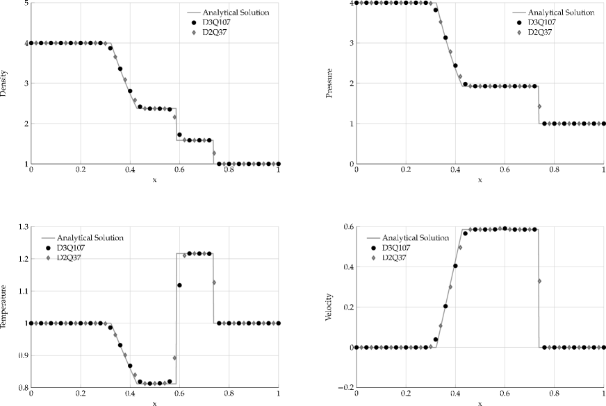
Figure 1: The simulation results of D2Q37, D3Q107, and the analytical resolutions at the time $t\!=\!0.1504$. The specific heat ratio is $\gamma\!=\!1.4$ and the parameter $\delta$ is $3$ in the case of 2D and $2$ in the case of 3D. The relaxation time is $\tau\!=\!2/3$. The initial condition of the left side is ${\rho\!=\!4,T\!=\!1,\bm{u}\!=\!0}$ and that of the right side is ${\rho\!=\!1,T\!=\!1,\bm{u}\!=\!0}$.

VI Conclusion

A new LB scheme associated with flexible specific heat ratio is proposed. A 2D LB model and a 3D LB model are derived via the Hermite expansion. The evolution equation of the distribution function is reduced to two evolution equations. The specific heat ratio obtained by the scheme is adjustable. The shock tube is employed to validate the proposed LB scheme. The simulation results agree with the analytical resolutions very well.

The LB models employed in the proposed scheme are derived via the Hermite quadrature, so the proposed scheme is more stable than the ones derived via the early method, which construct LB models in a try-error way. It is easy to construct LB models of any required level of accuracy.

For the proposed LB scheme, only the translational velocity is discretized and no other variables need to be discretized. So the LB scheme proposed by this work is much simpler than the existing schemes and much easier to be implemented.

References

• Alexander et al. (1993) F. J. Alexander, S. Chen,  and J. D. Sterling, Physical Review E Statistical Physics Plasmas Fluids & Related Interdisciplinary Topics 47, R2249 (1993).
• Qian (1993) Y. H. Qian, Journal of Scientific Computing 8, 231 (1993).
• Chen et al. (1994) Y. Chen, H. Ohashi,  and M. Akiyama, Phys. Rev. E 50, 2776 (1994).
• Philippi et al. (2006) P. C. Philippi, L. A. Hegele Jr, L. O. Dos Santos,  and R. Surmas, Physical Review E 73, 056702 (2006).
• Philippi et al. (2015) P. C. Philippi, D. Siebert, L. Hegele Jr,  and K. Mattila, Journal of the Brazilian Society of Mechanical Sciences and Engineering , 1 (2015).
• Mattila et al. (2014) K. K. Mattila, L. A. Hegele Júnior,  and P. C. Philippi, The Scientific World Journal 2014 (2014).
• Shan et al. (2006) X. Shan et al., Journal of Fluid Mechanics 550, 413 (2006).
• Shan et al. (2010) X. Shan et al., Physical Review E 81, 036702 (2010).
• Shim and Gatignol (2011) J. W. Shim and R. Gatignol, Physical Review E 83, 046710 (2011).
• Shim (2012) J. W. Shim, in Journal of Physics: Conference Series, Vol. 362 (IOP Publishing, 2012) p. 012011.
• Shim (2013a) J. W. Shim, Physical Review E 88, 053310 (2013a).
• Shim (2013b) J. W. Shim, Physical Review E 87, 013312 (2013b).
• Ansumali et al. (2003) S. Ansumali, I. V. Karlin,  and H. C. Öttinger, EPL (Europhysics Letters) 63, 798 (2003).
• Chikatamarla and Karlin (2006) S. S. Chikatamarla and I. V. Karlin, Physical review letters 97, 190601 (2006).
• Chikatamarla and Karlin (2009) S. S. Chikatamarla and I. V. Karlin, Physical Review E 79, 046701 (2009).
• Shi et al. (2001) W. Shi, W. Shyy,  and R. Mei, Numerical Heat Transfer: Part B: Fundamentals 40, 1 (2001).
• Kataoka and Tsutahara (2004) T. Kataoka and M. Tsutahara, Physical review E 69, 035701 (2004).
• Watari (2007) M. Watari, Physica A: Statistical Mechanics and its Applications 382, 502 (2007).
• Tsutahara et al. (2008) M. Tsutahara, T. Kataoka, K. Shikata,  and N. Takada, Computers & Fluids 37, 79 (2008).
• Lifschitz and Pitajewski (1983) E. Lifschitz and L. Pitajewski, in Textbook of theoretical physics. 10 (1983).
• Chu (1965a) C. Chu, Physics of Fluids (1958-1988) 8, 12 (1965a).
• Chu (1965b) C. Chu, Physics of Fluids (1958-1988) 8, 1450 (1965b).
• Sod (1978) G. A. Sod, Journal of Computational Physics 27, 1 (1978).
• Chen and Doolen (1998) S. Chen and G. D. Doolen, Annual review of fluid mechanics 30, 329 (1998).