The Chemical Abundance Structure of the Inner Milky Way: A Signature of “Upside-Down” Disk Formation?

Abstract

We present a model for the $[\alpha/{\rm Fe}]$-$[{\rm Fe}/{\rm H}]$ distribution of stars in the inner Galaxy, $3\,{\rm kpc}<R<5\,{\rm kpc}$, measured as a function of vertical distance $|z|$ from the midplane by Hayden et al. (2015, H15). Motivated by an “upside-down” scenario for thick disk formation, in which the thickness of the star-forming gas layer contracts as the stellar mass of the disk grows, we combine one-zone chemical evolution with a simple prescription in which the scale-height of the stellar distribution drops linearly from $z_{h}=0.8\,{\rm kpc}$ to $z_{h}=0.2\,{\rm kpc}$ over a timescale $t_{c}$, remaining constant thereafter. We assume a linear-exponential star-formation history, $\dot{M}_{*}(t)\propto te^{-t/t_{\rm sf}}$. With a star-formation efficiency timescale $\tau_{*}=M_{g}(t)/\dot{M}_{*}(t)=2\,{\rm Gyr}$, an outflow mass-loading factor $\eta=\dot{M}_{\rm out}(t)/\dot{M}_{*}(t)=1.5$, $t_{\rm sf}=3\,{\rm Gyr}$, and $t_{c}=2.5\,{\rm Gyr}$, the model reproduces the observed locus of inner disk stars in $[\alpha/{\rm Fe}]$-$[{\rm Fe}/{\rm H}]$ and the metallicity distribution functions (MDFs) measured by H15 at $|z|=0-0.5\,{\rm kpc}$, $0.5-1\,{\rm kpc}$, and $1-2\,{\rm kpc}$. Substantial changes to model parameters lead to disagreement with the H15 data; for example, models with $t_{c}=1\,{\rm Gyr}$ or $t_{\rm sf}=1\,{\rm Gyr}$ fail to match the observed MDF at high-$|z|$ and low-$|z|$, respectively. The inferred scale-height evolution, with $z_{h}(t)$ dropping on a timescale $t_{c}\sim t_{\rm sf}$ at large lookback times, favors upside-down formation over dynamical heating of an initially thin stellar population as the primary mechanism regulating disk thickness. The failure of our short-$t_{c}$ models suggests that any model in which thick disk formation is a discrete event will not reproduce the continuous dependence of the MDF on $|z|$ found by H15. Our scenario for the evolution of the inner disk can be tested by future measurements of the $|z|$-distribution and the age-metallicity distribution at $R=3-5\,{\rm kpc}$.

1. Introduction

Stars in the vicinity of the sun display a double-exponential distribution of heights $|z|$ above the disk midplane, often described as the superposition of a “thin disk” and “thick disk” (Gilmore & Reid 1983; Jurić et al. 2008). Young stars have cool kinematics that confine them to the thin disk, while stars with hotter kinematics are, on average, older, less metal rich, and enhanced in the $\alpha$-elements produced by core collapse supernovae. Abundance studies show that the distribution of [$\alpha$/Fe] is bimodal at solar or sub-solar [Fe/H], allowing chemical definition of “thin” and “thick” disk populations that display distinct kinematics (Bensby et al. 2003; Lee et al. 2011). A variety of mechanisms have been proposed for the origin of the thick disk, including debris of an accreted satellite (Abadi et al. 2003), heating of a pre-existing disk by satellites (Villalobos & Helmi 2008), gas-rich mergers or a turbulent gas-rich phase in the early star-forming disk (Brook et al. 2004; Bournaud et al. 2009; Forbes et al. 2012), or radial migration of stars outward from the kinematically hot inner disk (Schönrich & Binney 2009b). Two basic questions about the disk are: (1) were thick disk stars formed in a thick layer or heated over time from a thin distribution, and (2) was the formation of the thick disk a discrete event or extended over many orbital times?

In support of the “continuous” view, Bovy et al. (2012) show that mono-abundance populations in the disk, each defined by a narrow bin of $[{\rm Fe}/{\rm H}]$ and $[\alpha/{\rm Fe}]$, individually have exponential radial and vertical profiles. The superposition of multiple populations with different scale-heights gives rise to the double-exponential vertical profile observed for the full disk population and accounts for the correlation between [$\alpha$/Fe] and kinematics. Inspired by this finding, Bird et al. (2013) show that similar behavior arises for mono-age populations in a high-resolution hydrodynamic simulation of the formation of a Milky Way-like galaxy, starting from cosmological initial conditions. Furthermore, Bird et al. (2013) show that the oldest disk stars are born in a vertically thick distribution from a turbulently supported interstellar medium (ISM), in accord with previous numerical and analytic arguments about the influence of gravitational instability and feedback on the scale height of the star-forming gas disk (Bournaud et al. 2009; Forbes et al. 2012). They dub this scenario “upside-down” disk formation, by analogy to “inside-out” growth in which the disk scale length increases with time. While subsequent heating does increase the scale-height of older populations (Bird et al. 2013, fig. 19, and J. Bird et al., in prep.), cosmological simulations suggest that the distinction between the thick and thin disks was largely imprinted at birth.

In this paper, we show that the combination of upside-down disk formation with a simple chemical evolution model can naturally explain the observed [$\alpha$/Fe]-[Fe/H] distributions and metallicity distribution functions (MDFs) of the inner disk. The APOGEE survey (Majewski et al. 2016) has allowed mapping of the [$\alpha$/Fe]-[Fe/H] distribution over much of the Milky Way disk through high-resolution near-infrared spectroscopy of more than 100,000 evolved stars. In most regions of the Galaxy, as in the solar neighborhood, stars lie on two distinct sequences in [$\alpha$/Fe]-[Fe/H], though the locus of high-$\alpha$ stars appears to be independent of position within the disk (Hayden et al. 2015, hereafter H15). However, in the innermost radial zone mapped by H15, Galactocentric radius $3\,{\rm kpc}<R<5\,{\rm kpc}$, stars lie along a sequence that resembles the evolutionary track of a simple one-zone chemical evolution model (e.g., Talbot & Arnett 1971; Tinsley 1980). In such a model, low metallicity stars occupy a plateau in [$\alpha$/Fe] that reflects the characteristic yields of core collapse supernovae, averaged over the stellar initial mass function (IMF). Once Type Ia supernovae become an important source of enrichment, they further increase [Fe/H], but they drive down [$\alpha$/Fe] because they produce mainly iron-peak elements. The location of the “knee” where [$\alpha$/Fe] turns downward depends mainly on the star formation efficiency, while the value of [Fe/H] at late times depends mainly on the efficiency of galactic outflows, which controls the equilibrium between continuing enrichment from supernovae and loss of metals to stars and winds (Andrews et al. 2016,Weinberg et al. 2016, hereafter WAF). At $R=3-5$ kpc, most stars far from the midplane have enhanced [$\alpha$/Fe] and sub-solar [Fe/H], while most stars near the midplane have [$\alpha/\mathrm{Fe]}\approx 0$ and supersolar [Fe/H]. We will show that this distribution can be readily explained by one-zone chemical evolution in a vertically contracting disk.

Explaining the bimodal [$\alpha$/Fe]-[Fe/H] distribution seen at larger $R$ requires something more complex than the chemical evolution models considered here, such as mixing of stellar populations by radial migration (Sellwood & Binney 2002; Schönrich & Binney 2009a), sharp transitions in the Galaxy accretion and star formation history (Chiappini et al. 1997), or an increase of outflow efficiency at late times that induces reverse evolution towards lower [Fe/H] (WAF). Here we focus on the inner disk, where simple models appear applicable. We suspect that the more complex structure of the outer disk arises because radial migration has a larger impact there, while the inner disk is dominated by stars that remain close to their birth radius. Tentative support for this view comes from the modeling of MDFs presented by H15 (see their Figure 10). A full model for the formation and evolution of the Milky Way disk must account for its full spatial and chemo-dynamical structure and explain the distributions of elements that trace different nucleosynthetic pathways. This paper presents idealized models intended to highlight one aspect of this evolution.

2. Data and sample selection

Our data sample is a subset of that studied by H15, drawn from the APOGEE survey (Majewski et al. 2016) of the Sloan Digital Sky Survey III (SDSS-III, Eisenstein et al. 2011). It consists of red giant and sub-giant stars with elemental abundances inferred from infrared (H-band) spectroscopy with spectral resolution $\lambda/\Delta\lambda\approx 20,000$ (Nidever et al. 2015). Elemental abundances are inferred from the APOGEE Stellar Parameters and Chemical Abundances Pipeline (ASPCAP; García Pérez et al. 2016). In brief, the parameters of each star are determined by $\chi^{2}$ minimization across the full spectrum, using 6-parameter model grids: $T_{\mathrm{eff}}$, $\log g$, an overall metallicity [M/H], scalings of $\alpha$-elements relative to the overall metallicity [$\alpha$/M], and individually varied abundances of C and N. With free variations of $\alpha$, C, and N, the metallicity M is responsive mainly to iron peak elements. We (like H15) refer to [$\alpha$/M] and [M/H] by the more conventional labels [$\alpha$/Fe] and [Fe/H]. We apply the same cuts as H15, summarized here in Table 1, to select main sample, evolved stars with high-quality abundance determinations. These abundances are the ones provided in SDSS DR12 (Alam et al. 2015; Holtzman et al. 2015). Further details of APOGEE field and target selection can be found in Zasowski et al. (2013).

H15 estimate distances from spectroscopically determined stellar parameters, PARSEC isochrones (Bressan et al. 2012), and extinction-corrected apparent magnitudes (see H15 and Holtzman et al. 2015 for details). They use these distances to assign stars to bins in Galactocentric radius $R$ and vertical distance from the midplane $|z|$. In this paper we concentrate on H15’s innermost radial bin 3 kpc $<R<$ 5 kpc, where stars lie along what is plausibly a single evolutionary track. After the cuts listed in Table 1 we are left with 3753 stars: 2435 at $|z|=0-0.5\,{\rm kpc}$, 849 at $|z|=0.5-1.0\,{\rm kpc}$, and 469 at $|z|=1.0-2.0\,{\rm kpc}$. The top panels of Figure 1 plot the metallicity distribution functions (MDFs) of stars in these three vertical layers, and the bottom panels plot the distribution of stars in the [$\alpha$/Fe]-[Fe/H] plane, together with the evolutionary track described in the following section. Equivalent information in different format appears in Figures 4 and 5 of H15.

Table 1Cuts made on APOGEE data for sample selection

Cuts	Notes
3 kpc $<R<$ 5 kpc	Inner annulus of H15
$1.0<\log g<3.8$	Choose giants only
3500 K $<T_{\mathrm{eff}}<$ 5500 K	High quality abundances
S/N $>80$	”
APOGEE_TARGET1 bits $\in$ 11,12,13	Main survey targets only
ASPCAPFLAG bits $\notin$ 23	Remove bad stars

3. Chemical Evolution Model

We adopt oxygen as the representative $\alpha$-element in our theoretical model. The H15 measurements depend on several $\alpha$-elements with oxygen dominant among them. Within our model, the defining characteristic of $\alpha$ elements is that they are produced by core collapse supernovae only, with a yield that is independent of metallicity.

We calculate chemical evolution within a single galactic zone according to the following specifications:

1. The galactic zone consists of a supply of gas out of which stars are formed over time. This gas is initially pristine hydrogen and helium, and it is homogeneously mixed at all times. Any new metals introduced by supernovae are immediately mixed into the existing gas supply.

2. Stars are formed from the gas supply with a constant efficiency $\dot{M}_{*}/M_{g}$, which we specify in terms of a star formation efficiency (SFE) timescale $\tau_{*}=M_{g}/\dot{M}_{*}$. We choose $\tau_{*}=2.0$ Gyr, based on the observationally inferred timescale for molecular gas in local disk galaxies (Leroy et al. 2008).

3. The star formation rate (SFR) evolves in a linear-exponential fashion, i.e.,

   $$\dot{M}_{*}(t)=\dot{M}_{*}(t_{\rm sf})\times\left(\frac{t}{t_{\rm sf}}\right)e^{-t/t_{\rm sf}}~{},$$ (1)

   where $t_{\rm sf}$ is the star formation timescale. Together with assumption 2, this implies a linear-exponential form for the gas supply $M_{g}(t)=\tau_{*}\dot{M}_{*}(t)$. We consider several different values for $t_{\rm sf}$. The Appendix shows results for an exponential star formation history, but the linear-exponential model corresponds better to the predictions of galaxy formation simulations (Simha et al. 2014), and it yields a somewhat better fit to the H15 data.

4. Outflow of gas from the zone, due to stellar feedback, occurs at a rate $\dot{M}_{\mathrm{out}}$. We parameterize outflow efficiency with the mass-loading factor $\eta$, such that $\eta=\dot{M}_{\mathrm{out}}/\dot{M}_{*}$. We adjust the value of $\eta$ depending on $t_{\rm sf}$ to produce similar peaks in the [Fe/H] distribution (see discussion below).

5. Each population of stars forms with masses distributed according to a Kroupa (2001) IMF, which prescribes a double power-law form for

   $$\zeta(M)\propto\frac{dN(M)}{dM}$$ (2)

   with slopes $a$ and $b$ above and below $cM_{\odot}$. We truncate the IMF at $M_{\rm min}=0.08M_{\odot}$ and $M_{\rm max}=100M_{\odot}$.

6. There are two sources of new metal production: core-collapse supernovae (CCSNe) and Type Ia supernovae (SNIa). We define the yield parameters $m_{\rm O}^{\rm CC}$, the mass of oxygen produced by CCSNe per unit mass of star formation, $m_{\rm Fe}^{\rm CC}$, the corresponding quantity for iron, and $m_{\rm Fe}^{\rm Ia}$, the mass of iron produced by SNIa over a time interval 12.5 Gyr per unit mass of star formation. We adopt $m_{\rm O}^{\rm CC}=0.015$ and $m_{\rm Fe}^{\rm CC}=0.0012$, based on a Kroupa IMF and the CCSN yields of Chieffi & Limongi (2004) and Limongi & Chieffi (2006). We adopt $m_{\rm Fe}^{\rm Ia}=0.0017$ based on the SNIa rate of Maoz et al. (2012) and an iron yield of $0.77M_{\odot}$ (Iwamoto et al. 1999) per supernova (see Andrews et al. 2016 for more detailed discussion). These yields are defined to be net quantities: they do not include the amount of oxygen and iron incorporated into the stellar population from the ISM at birth, but only the newly produced amounts of these elements.

7. CCSNe go off instantaneously upon the birth of a stellar population; this is a reasonable approximation because we adopt star formation histories that are smooth on much longer timescales. However, it does assume that the “lock up” of metals in the warm or hot phases of the ISM (Schönrich & Binney 2009a) can be ignored.

8. SNIa follow a power-law delay time distribution (DTD) after a minimum delay time $t_{d}$:

   $$R(t)=\begin{cases}R_{0}t^{-1.1}&t>t_{d}\\ 0&t<t_{d}~{}.\end{cases}$$ (3)

   The form is based on Maoz et al. (2012), and the normalization $R_{0}$ cancels out of our calculations once we have specified the iron yield $m_{\rm Fe}^{\rm Ia}$. We adopt $t_{d}=0.15\,{\rm Gyr}$.

9. A star of mass $M$ lives for a time $t_{*}=10\mathrm{\,Gyr}\times(M/M_{\odot})^{-3.5}$, then returns to the ISM a mass of gas $M-M_{\rm rem}$ with the same chemical composition the star had at birth. (Stars above $8M_{\odot}$ additionally return elements with the CCSN net yields described above.) The remnant mass as a function of initial mass is

   $$M_{\rm rem}(M)=\begin{cases}0.394M_{\odot}+0.109M&M<8M_{\odot}\\ 1.44M_{\odot}&M>8M_{\odot}~{}.\end{cases}$$ (4)

   (see Kalirai et al. 2008). The lifetime formula can be inverted to yield the main sequence turnoff mass as a function of time:

   $$M_{\rm to}(t)=\left(\frac{t}{10\mathrm{\,Gyr}}\right)^{-1/3.5}M_{\odot}~{}.$$ (5)

With the assumptions of point 9, the fraction of a mass of stars formed in a short interval at time $t^{\prime}$ that has been recycled to the ISM by time $t$ is

$$F_{\rm rec}(t,t^{\prime})=\frac{\int_{M_{\rm to}(t-t^{\prime})}^{M_{\rm max}}M\zeta(M)\left[1-f_{\rm rem}(M)\right]\,dM}{\int_{M_{\rm min}}^{M_{\rm max}}M\zeta(M)\,dM}~{},$$ (6)

where $f_{\rm rem}(M)=M_{\rm rem}(M)/M$ is the fraction of a star of initial mass $M$ that is left in the stellar remnant. While our lifetime formula is inaccurate at high masses, it adequately captures the important behavior, which is that high mass stars recycle their envelopes quickly compared to the timescales for SNIa enrichment and variation of the SFR. For a Kroupa IMF, the recycled mass fraction is $r=F_{\rm rec}(t,t^{\prime})=0.37$, 0.40, and 0.45 for $t-t^{\prime}=1$, 2, and 10 Gyr, respectively. The difference in chemical evolution between our complete time-dependent recycling and an instantaneous approximation with $r=0.4$ is small (see fig. 7 of WAF).

With these assumptions in place, we may write down the differential equations governing the amount of oxygen and iron in the ISM. Metals are injected into the ISM by CCSNe, SNIa, and recycling, and they are removed from the ISM by star formation and outflows. For oxygen,

$$\begin{split}\dot{M}_{\rm O}&=m_{\rm O}^{\rm CC}\dot{M}_{*}-\dot{M}_{*}Z_{\rm O}-\eta\dot{M}_{*}Z_{\rm O}\\ &\hskip 22.76219pt+\int_{0}^{t}\dot{M}_{*}(t^{\prime})Z_{\rm O}(t^{\prime})\dot{F}_{\rm rec}(t,t^{\prime})\,dt^{\prime}\\ &=m_{\rm O}^{\rm CC}\frac{M_{g}}{\tau_{*}}-(1+\eta)\frac{M_{\rm O}}{\tau_{*}}+\int_{0}^{t}\frac{M_{\rm O}(t^{\prime})}{\tau_{*}}\dot{F}_{\rm rec}(t,t^{\prime})\,dt^{\prime}~{},\end{split}$$ (7)

where $Z_{\rm O}=M_{\rm O}/M_{g}$ is the oxygen mass fraction and $\dot{F}_{\rm rec}(t,t^{\prime})$ is the derivative of equation (6) with respect to $t$. For iron we have the additional contribution of SNIa:

$$\begin{split}\dot{M}_{\rm Fe}&=m_{\rm Fe}^{\rm CC}\frac{M_{g}}{\tau_{*}}-(1+\eta)\frac{M_{\rm Fe}}{\tau_{*}}+\int_{0}^{t}\frac{M_{\rm Fe}(t^{\prime})}{\tau_{*}}\dot{F}_{\rm rec}(t,t^{\prime})\,dt^{\prime}\\ &\hskip 22.76219pt+m_{\rm Fe}^{\rm Ia}\frac{\int_{0}^{t}R(t-t^{\prime})M_{g}(t^{\prime})/\tau_{*}\,dt^{\prime}}{\int_{0}^{\infty}R(t^{\prime})\,dt^{\prime}}~{}.\end{split}$$ (8)

We solve these equations for oxygen and iron evolution with a numerical code that uses simple Euler integration to evolve the zone from $t=0$ to $t=12.5$ Gyr, with a step size of $\Delta t=10$ Myr; that is,

$$M_{\mathrm{X},i}=M_{\mathrm{X},i-1}+\dot{M}_{\mathrm{X},i-1}\Delta t~{}.$$ (9)

We evaluate the recycling term from the cumulative values of $F_{\rm rec}(t,t^{\prime})$ at the beginning and end of the step. We prescribe a star formation history rather than an infall history (see Vincenzo et al. 2016 for a mathematical discussion of the relation between these), and the gas mass is therefore implicitly specified by $M_{g}(t)=\tau_{*}\dot{M}_{*}(t)$, with no need to integrate it separately.

Our assumptions are similar to those of many one-zone chemical evolution models, and they closely follow those adopted for analytic modeling by WAF. WAF show that when the integral recycling terms in equations (7) and (8) are replaced by the instantaneous approximation $rM_{X}(t)/\tau_{*}$, then the resulting equations for oxygen and iron evolution can be solved analytically if one adopts an exponential DTD for SNIa enrichment and a constant, exponential, or linear-exponential star formation history. These solutions show that for a wide range of model parameters the values of $[{\rm Fe}/{\rm H}]$ and $[{\rm O}/{\rm Fe}]$ converge within a few Gyr to “equilibrium” values at which sources and sinks balance, reproducing numerical results (Andrews et al. 2016). The equilibrium $[{\rm Fe}/{\rm H}]$ depends mainly on yields and on the value of $\eta$, while the equilibrium $[{\rm O}/{\rm Fe}]$ depends mainly on yields. The importance of equilibrium, and the key role of outflow efficiency in regulating abundances, has been highlighted in theoretical studies of the galaxy mass-metallicity relation (Finlator & Davé 2008; Peeples & Shankar 2011; Davé et al. 2012).

In the cosmological simulation of Bird et al. (2013), the median height of the star-forming gas layer decreases from about 0.8 kpc to about 0.2 kpc between $t\approx 2\,{\rm Gyr}$ and $t\approx 6\,{\rm Gyr}$, as the ratio of rotational velocity to turbulent vertical velocity grows rapidly. After that, the gas layer continues to get thinner, but at a much slower rate. Rather than mimic a single simulation, we adopt an idealized model in which the scale-height $z_{h}$ of newly formed stars decreases linearly from 0.8 kpc to 0.2 kpc over a collapse timescale $t_{c}$ and remains constant thereafter:

$$z_{h}(t,t_{c})=\begin{cases}0.8\,{\rm kpc}-0.6\,{\rm kpc}\times(t/t_{c})&t\leq t_{c},\\ 0.2\,{\rm kpc}&t>t_{c}~{}.\end{cases}$$ (10)

Figure 2 compares these scale-height histories to the star formation histories for the values of $t_{c}$ and $t_{\rm sf}$ that we consider below. In a model where gravitationally driven turbulence of a gas rich disk governs both the thickness of the gas layer and the efficiency of star formation (Bournaud et al. 2009; Forbes et al. 2012), we might expect the collapse time to be linked to the evolution of the SFR. We do not impose this condition a priori, but we find that our fits to the H15 data prefer comparable collapse and star-formation timescales.

We evolve our model for 12.5 Gyr. As noted previously, we choose the gas supply so that the star formation rate is

$$\frac{dN_{*}}{dt}\propto\frac{M_{g}(t)}{\tau_{*}}\propto te^{-t/t_{\rm sf}}~{}.$$ (11)

The $\Delta N_{*}=\Delta t\times(dN_{*}/dt)$ stars formed in a given timestep are assigned $z$ values drawn from the distribution

$$h(z,t_{c})\propto e^{-z/z_{h}(t,t_{c})}~{},$$ (12)

where $z_{h}(t,t_{c})$ is given by equation (10). Thus, for a given $t_{c}$ the fraction of stars formed at time $t$ with $z_{1}<z<z_{2}$ is given by

$$\frac{N_{z_{1}\rightarrow z_{2}}}{N_{\mathrm{tot}}}=\frac{\int_{z_{1}}^{z_{2}}{e^{-z/z_{h}(t,t_{c})}dz}}{\int_{0}^{\infty}{e^{-z/z_{h}(t,t_{c})}dz}}~{}.$$ (13)

We ignore any subsequent changes to the vertical structure of the disk, e.g., from dynamical heating or adiabatic compression, a point we return to at the end of §4. Each star formed is assigned oxygen and iron abundances according to the abundances in the ISM at time $t$, which are determined by the chemical evolution model described above. Scatter is added to these values, drawn from a Gaussian distribution with $\sigma=0.05$ dex. We implement scatter partly to enable better visual interpretation of our plots and partly to mimic effects of observational errors.

4. Model Comparison

Figure 3 displays the predicted distribution of stars in $[{\rm O}/{\rm Fe}]-[{\rm Fe}/{\rm H}]$, in the form of color-coded 2-d historgrams, in the same three vertical layers used in Figure 1. We consider $t_{c}$ values of 1.0, 2.5, and 4.5 Gyr and $t_{\rm sf}$ values of 1.0, 3.0, and 6.0 Gyr (see Fig. 2), making nine models in total. In each panel, the central track shows the model abundances calculated without scatter, and colored points mark the abundance values at $t=0.1$, 0.5, 1.0, 2.0, 5.0, and 10.0 Gyr. The tracks and colored points are identical in a given column of the plot because $z$ and $t_{c}$ do not enter into the chemical evolution. As explained by WAF, equilibrium abundances depend mainly on yields and $\eta$ if $t_{\rm sf}$ is long, but as $t_{\rm sf}$ approaches the gas depletion time $\tau_{*}/(1+\eta-r)$ the equilibrium abundance grows, and the approach to equilibrium gets slower. For $t_{\rm sf}=6.0\,{\rm Gyr}$ and $3.0\,{\rm Gyr}$, we have adopted $\eta=1.17$ and 1.50, so that both models yield $[{\rm Fe}/{\rm H}]\approx+0.25$ at $t=10\,{\rm Gyr}$. For $t_{\rm sf}=1.0\,{\rm Gyr}$ we choose $\eta=2.83$, which gives $[{\rm Fe}/{\rm H}]\approx+0.25$ at $t=5\,{\rm Gyr}$, but because of the rapid truncation of the SFR most stars form below this metallicity. Tracks and timestamped abundances are fairly similar in the $t_{\rm sf}=6.0$ and $3.0\,{\rm Gyr}$ models, though one can see the slightly slower approach to equilibrium for $t_{\rm sf}=3.0\,{\rm Gyr}$. The evolutionary track and, especially, abundance vs. time are significantly different for $t_{\rm sf}=1.0\,{\rm Gyr}$.

As shown previously in Figure 1, the evolutionary track of our $t_{\rm sf}=3.0\,{\rm Gyr}$ model follows the observed locus of H15 stars quite well. This agreement indicates that, given our adopted CCSN and SNIa yields, our adopted values of $\tau_{*}$ and $\eta$ are reasonable. We note in particular that a much higher (lower) star formation efficiency would drive the knee of the evolutionary track to higher (lower) $[{\rm Fe}/{\rm H}]$, in disagreement with the data, though we have not investigated the degree to which a change in $\tau_{*}$ could be compensated by changes in the star formation history or SNIa DTD. The predicted $[{\rm O}/{\rm Fe}]$ at high $[{\rm Fe}/{\rm H}]$ is slightly sub-solar, while the APOGEE measurements yield solar $[\alpha/{\rm Fe}]$. Given the uncertainties in observational calibrations, solar abundance values, and supernova yields, we do not ascribe much significance to this discrepancy, but models with longer $t_{\rm sf}$ and thus higher equilibrium $[{\rm O}/{\rm Fe}]$ would fit the data better with other assumptions held fixed. Physically, a more rapidly declining star formation history leads to lower $[{\rm O}/{\rm Fe}]$ at late times because the ratio of CCSNe to SNIa is lower.

The choices of $t_{c}$ and $t_{\rm sf}$ affect the distribution of stars, both along the tracks and among layers of the disk. Examining the middle column isolates the effect of $t_{c}$. The most distinctive impact can be seen in the $|z|=1-2\,{\rm kpc}$ layers of the $t_{c}=1.0$ and $2.5\,{\rm Gyr}$ models. For the shorter collapse timescale, the distribution of stars in this layer is bimodal, with one group of stars near the knee of the track (formation times centered at $t\approx 0.5\,{\rm Gyr}$) and a second group near the end of the track (formation times centered at $t\approx 5\,{\rm Gyr}$). The first group forms during disk collapse, when the scale-height is still fairly high. By $t=1.0\,{\rm Gyr}$ the scale-height has dropped to 0.2 kpc, and although the SFR between $t=1\,{\rm Gyr}$ and $3\,{\rm Gyr}$ is high, only a modest fraction of all stars are formed in this interval (see Figure 2), and a small fraction of these have $|z|>1\,{\rm kpc}$. The disk remains thin at later times, but more than 60% of the stars form between 3 and 10 Gyr, and the high-$|z|$ tail of this population is sufficient to produce the second group of stars, at high $[{\rm Fe}/{\rm H}]$. The central model, with $t_{c}=2.5\,{\rm Gyr}$, still has a bimodal distribution of stars in the high-$|z|$ later, but now the $\alpha$-enhanced low metallicity group is far more prominent because the disk collapse is slower, and more stars form while the scale-height remains high.

Other differences in the middle column of Figure 3 are more subtle but follow similar trends. In the high-$|z|$ layer, the mean metallicity of the low-$[{\rm Fe}/{\rm H}]$ group increases as $t_{c}$ increases, since the population can evolve toward higher metallicity before the disk contracts to low scale-height. For $t_{c}=1.0\,{\rm Gyr}$, the mid-$|z|$ layer is dominated by stars formed at late times when the disk is thin, but for $t_{c}=4.5\,{\rm Gyr}$ this layer is dominated by intermediate-age stars formed during collapse. The central, $t_{c}=2.5\,{\rm Gyr}$ model has the broadest distribution of age and $[{\rm Fe}/{\rm H}]$ in the mid-$|z|$ layer because these two groups join to make a single continuous distribution. The low-$|z|$ layers appear similar in all three models because a large fraction of stars form after the disk has reached its 0.2 kpc scale-height.

Each 2-d histogram in Figure 3 is normalized relative to the maximum density in the same layer, similar to the analogous figure of H15 (their fig. 4). However, the relative number of stars in the higher $|z|$ layers depends strongly on $t_{c}$ and to some degree on $t_{\rm sf}$; for example, in the central column the fraction of stars with $|z|=1-2\,{\rm kpc}$ increases from 1% to 5% between the $t_{c}=1.0$ and $4.5\,{\rm Gyr}$ models. The relative numbers of stars in the H15 sample are strongly shaped by the survey strategy and selection function of APOGEE, so we cannot use them as a model test. A measurement of the $|z|$-distribution of stars with $R=3-5\,{\rm kpc}$ provide an additional diagnostic for distinguishing models, a point we return to in the discussion of Figure 8 below.

The impact of $t_{\rm sf}$ can be seen by looking across the middle ($t_{c}=2.5\,{\rm Gyr}$) row of Figure 3. A shorter $t_{\rm sf}=1.0\,{\rm Gyr}$ (left column) leads to a broader distribution of $[{\rm Fe}/{\rm H}]$ in the high-$|z|$ layer, since rapid early star formation allows greater chemical enrichment before disk contraction. The low-$|z|$ layer is populated mainly by stars formed between $t=1$ and $5\,{\rm Gyr}$, but despite the narrower age range, the metallicity range (roughly $[{\rm Fe}/{\rm H}]=-0.5$ to $+0.25$) is broader than that of the corresponding layer for $t_{\rm sf}=3.0\,{\rm Gyr}$. Moving to $t_{\rm sf}=6.0\,{\rm Gyr}$ (right column) leads to a much stronger concentration of low-$|z|$ stars near the equilibrium metallicity, both because the approach to equilibrium is faster for longer $t_{\rm sf}$ and because this model forms a larger fraction of its stars at late times (see Figure 2). At high $|z|$ this model shows a bimodal distribution similar to that of the ($t_{\rm sf}=3.0\,{\rm Gyr},t_{c}=1.0\,{\rm Gyr}$) model discussed previously, again with a low-$[{\rm Fe}/{\rm H}]$ group formed during disk collapse and a high-$[{\rm Fe}/{\rm H}]$ group that is the high-$|z|$ tail of the much larger number of stars formed at late times with a 0.2 kpc scale-height. Most of the models in Figure 3 show some degree of this bimodality at high $|z|$, but the relative importance of the two groups depends on the specific values of $t_{\rm sf}$ and $t_{c}$. More generally, while there is some tradeoff between these two parameters, their impact is not strongly degenerate once all three layers are considered.

Figure 4 plots metallicity distribution functions (MDFs), the fraction of stars in bins of $[{\rm Fe}/{\rm H}]$, for the same nine models and three $|z|$-layers shown in Figure 3. Because all stars in a given model lie along a single evolutionary track, the one-dimensional MDF together with the track itself retains all of the information from Figure 3. The MDF allows easier comparison to the H15 measurements, shown by the orange curves in Figure 4. The $t_{\rm sf}=1.0\,{\rm Gyr}$ models are a consistently poor match to the data in the low-$|z|$ layer, predicting MDFs that are too broad and too symmetric. Changes to $\eta$, supernova yields, or $\tau_{*}$ could shift the centroid of the MDF, but the broad and symmetric shape is a generic consequence of the short star-formation timescale (WAF; Andrews et al. 2016). The observed MDF at low $|z|$ instead shows the peaked, negatively skewed form expected when continuing infall allows a large fraction of stars to form near the equilibrium abundance, and the $t_{\rm sf}=3.0\,{\rm Gyr}$ and $t_{\rm sf}=6.0\,{\rm Gyr}$ models reproduce it much better. The high-$|z|$ MDF of these models is nearly always bimodal, but the relative amplitudes of the low-$[{\rm Fe}/{\rm H}]$ and high-$[{\rm Fe}/{\rm H}]$ peaks varies strongly from one $(t_{\rm sf},t_{c})$ combination to another. The data do not show a clear bimodality in this layer, and the $(t_{\rm sf}=3.0\,{\rm Gyr},t_{c}=2.5\,{\rm Gyr})$ model, for which the two peaks merge into a continuous broad distribution, provides the best match to the data. This model and the $(t_{\rm sf}=3.0\,{\rm Gyr},t_{c}=4.5\,{\rm Gyr})$ model also provide the best match to the $|z|=0.5-1\,{\rm kpc}$ MDF, for which models with shorter $t_{c}$ or longer $t_{\rm sf}$ predict too many high-$[{\rm Fe}/{\rm H}]$ stars.

Table 2Statistical quantities used to compare model MDFs to the H15 data; $x_{i}$ is the value of [Fe/H] in the $i$th bin, $N$ is the number of bins, $N_{*,i}$ is the number of stars in the $i$th bin, and $f_{*,i}=N_{*,i}/N_{*,{\rm tot}}$ is the fraction of stars in the $i$th bin.

Name	Equation
$\Delta^{2}$	$\sum_{i=0}^{N}\left(f^{\rm data}_{*,i}-f^{\rm model}_{*,i}\right)^{2}$
Mean	$\bar{x}=\frac{1}{N}\sum_{i=0}^{N}{x_{i}N_{*i}}$
Variance	$\sigma^{2}=\frac{1}{N}\sum_{i=0}^{N}{(x_{i}-\bar{x})^{2}N_{*i}}$
Skewness	$\frac{1}{N}\sum_{i=0}^{N}{\left[(x_{i}-\bar{x})/\sigma\right]^{3}N_{*i}}$
Kurtosis	$\frac{1}{N}\sum_{i=0}^{N}{\left[(x_{i}-\bar{x})/\sigma\right]^{4}N_{*i}}-3$

To quantify the level of agreement seen in Figure 4, we compute the squared difference of the MDF histograms

$$\Delta^{2}=\sum_{i=0}^{N}\left(f^{\rm data}_{*,i}-f^{\rm model}_{*,i}\right)^{2}~{},$$ (14)

where the sum is over the $N=75$ $[{\rm Fe}/{\rm H}]$ bins. Figure 5 plots these values for the nine models in each of the three $|z|$ layers. In the low-$|z|$ layer, the $t_{\rm sf}=1.0\,{\rm Gyr}$ model performs very poorly, while the $t_{\rm sf}=3.0\,{\rm Gyr}$ and $6.0\,{\rm Gyr}$ models reproduce the data about equally well, with almost no dependence on $t_{c}$. In the mid-$|z|$ layer, the $t_{\rm sf}=6.0\,{\rm Gyr}$ model fares poorly, especially for low $t_{c}$, and the $t_{\rm sf}=3.0\,{\rm Gyr}$ model performs best at all $t_{c}$. The high-$|z|$ layer strongly disfavors $t_{c}=1\,{\rm Gyr}$, for any $t_{\rm sf}$, and it again disfavors the $t_{\rm sf}=6.0\,{\rm Gyr}$ models at all $t_{c}$. Overall, the $t_{\rm sf}=3.0\,{\rm Gyr}$ models with $t_{c}=2.5$ or $4.5\,{\rm Gyr}$ are clearly the most successful, with $t_{c}=2.5\,{\rm Gyr}$ slightly preferred. We have not attempted to formally evaluate parameter uncertainties or a global goodness-of-fit, in part because our models seem too idealized to warrant such an approach. In particular, a global $\chi^{2}$ or maximum likelihood statistic would assign the most weight to the low-$|z|$ MDF, which is based on the most stars and thus has the smallest statistical errors, but given that our models are likely incomplete, the level of agreement in the mid-$|z|$ and high-$|z|$ layers is a better diagnostic of star formation and disk collapse timescales than small improvements in reproducing the low-$|z|$ data. A formal fitting procedure would also require accounting for systematic uncertainties in the abundance data and for the influence of APOGEE’s evolved star selection on the MDF.

Figure 6 plots the first four moments of the MDFs — mean, variance, skewness, and kurtosis — for the nine models and the data in each $|z|$-layer. Our precise definitions of these moments are given in Table 2. In each panel, the horizontal black line marks the measured moment for the data and the grey band marks the 1-$\sigma$ error on the mean, determined from 20 bootstrap resamplings of the original data set. Because the MDFs are sometimes strongly non-Gaussian (e.g., bimodal), even four moments do not fully characterize their shapes. Overall, the moments comparison also shows the $t_{\rm sf}=3.0\,{\rm Gyr}$ models with $t_{c}=2.5\,{\rm Gyr}$ or $4.5\,{\rm Gyr}$ to be the most successful. However, the $t_{\rm sf}=6.0\,{\rm Gyr}$ models give better agreement with the skewness of the low-$|z|$ MDF, and the rejection of $t_{c}=1.0\,{\rm Gyr}$ models is much more resounding for the $\Delta^{2}$ statistic than it is for MDF moments.

Figure 7 returns to a more qualitative comparison between our central model ($t_{\rm sf}=3.0\,{\rm Gyr}$,$t_{c}=2.5\,{\rm Gyr})$ and the H15 data. In each layer, we select a number of stars similar to that in the H15 data, and we plot them (including the 0.05-dex of added scatter in $[{\rm O}/{\rm Fe}]$ and $[{\rm Fe}/{\rm H}]$) in the same manner as the lower three panels of Figure 1, which we repeat here to allow direct visual comparison. The model effectively reproduces the spread and shifting centroid of the metallicity distribution in each layer. As previously noted, the model predicts a slightly lower $[\alpha/{\rm Fe}]$ at the highest $[{\rm Fe}/{\rm H}]$, possibly a symptom of a $t_{\rm sf}$ that is too low, or of incorrect supernova yields, or incorrect APOGEE calibration at super-solar $[{\rm Fe}/{\rm H}]$. In the low-$|z|$ layer, the data show a hint of bimodality in $[\alpha/{\rm Fe}]$ at slightly sub-solar $[{\rm Fe}/{\rm H}]$, which is not predicted by the model. This hint of two distinct sequences could be a sign that radial migration has moved some low-$\alpha$ stars from the lower metallicity outer disk into the $R=3-5\,{\rm kpc}$ annulus (Schönrich & Binney 2009a), the complement to the explanation that H15 advance for the skew-positive shape of the midplane MDF at larger radii.

Figure 8 displays the vertical distribution $dN_{*}/dz$ predicted by all nine models. For the central model, $dN_{*}/dz$ is well described (up to $|z|=4\,{\rm kpc}$) by the sum of two exponentials with scale-heights of 0.2 kpc and 0.6 kpc, with equal normalization at $|z|=1.036\,{\rm kpc}$. Although our model starts with $z_{h}=0.8\,{\rm kpc}$, few stars form at very early times, so the effective scale-height of the “thick disk” component is lower. We have arbitrarily normalized all of these distributions to $dN_{*}/dz=1\,{\rm kpc}^{-1}$ at $z=0$. With the same mid-plane density, models that have longer $t_{c}$ at a given $t_{\rm sf}$ produce more stars at high $|z|$, as expected. In the solar neighborhood, the Jurić et al. (2008) decomposition of the M-dwarf population implies thin- and thick-disk scale-heights of 0.3 kpc and 0.9 kpc, respectively, with equal normalizations at $|z|=0.95\,{\rm kpc}$. We do not know of any vertical density profile measurements at $R=3-5\,{\rm kpc}$ where our models apply, and the Jurić et al. (2008) sample is too local for reliable extrapolation to this Galactocentric radius. Such a measurement would be a valuable additional diagnostic for the scenario presented here. In particular, our choices of $z_{h}=0.8\,{\rm kpc}$ and 0.2 kpc for the initial and final scale-heights of our contracting disk, while loosely motivated by the Bird et al. (2013) cosmological simulation, are somewhat arbitrary. Additional constraints from a vertical profile measurement might allow these quantities to be treated as adjustable model parameters rather than fixed a priori.

We have framed our model in terms of upside-down disk formation, with $z_{h}(t)$ representing the scale-height of the star-forming gas layer over time. However, a model in which all stars formed in a thin layer and dynamical heating puffed up the older stellar populations would make identical predictions if it produced the same $z_{h}(t)$. The principal argument that favors a contracting gas layer over stellar heating as the predominant mechanism governing disk thickness is that the $z_{h}(t)$ of our most successful models is a plausible outcome of the upside-down scenario, with disk contraction occurring as the disk transitions from gas-dominated to having comparable gas and stellar mass. For $\tau_{*}=2.0\,{\rm Gyr}$, $t_{\rm sf}=3.0\,{\rm Gyr}$, and a recycling fraction $r=0.4$, the ratio of stellar mass to gas mass is 0.5 at $t=2.5\,{\rm Gyr}$ and 1.2 at $t=4.5\,{\rm Gyr}$. In a heating scenario, these $z_{h}(t)$ histories would require a heating mechanism that is sharply peaked at early times (see Figure 2), rather than the continuous, roughly power-law dependence on lookback time that is predicted by typical dynamical heating mechanisms (Hänninen & Flynn 2002). However, we have not explicitly demonstrated that a conventional heating model is inconsistent with the H15 data. Even in an upside-down scenario, dynamical heating is likely influence the scale-height of populations at the present day (Bird et al. 2013, Fig. 19; J. Bird et al., in prep.).

We have not explicitly examined scenarios in which disk heating is a sudden event, as might result from a satellite merger. Given the drastic failure of our $t_{c}=1.0\,{\rm Gyr}$ models, however, we think it unlikely that a discrete heating scenario can reproduce the steady trend of the H15 abundance distributions with $|z|$.

5. Conclusions

Motivated by an “upside-down” scenario for thick disk formation, in which the height of the star-forming gas layer contracts as the stellar mass of the disk grows (Bournaud et al. 2009; Forbes et al. 2012; Bird et al. 2013), we have presented a simple model to explain the $|z|$-dependent $[\alpha/{\rm Fe}]$-$[{\rm Fe}/{\rm H}]$ distributions of inner disk stars ($3\,{\rm kpc}<R<5\,{\rm kpc}$) measured by H15 from the APOGEE survey. The H15 inner disk stars appear to lie along a single evolutionary track, with most high-$|z|$ stars at sub-solar $[{\rm Fe}/{\rm H}]$ and $[\alpha/{\rm Fe}]=0.2-0.4$, most low-$|z|$ stars at super-solar $[{\rm Fe}/{\rm H}]$ and solar $[\alpha/{\rm Fe}]$, and mid-$|z|$ stars spread broadly over the $[{\rm Fe}/{\rm H}]$ range $-0.5$ to $+0.25$. Our model combines one-zone chemical evolution with a disk that contracts linearly from a scale-height of $z_{h}=0.8\,{\rm kpc}$ to $z_{h}=0.2\,{\rm kpc}$ over a timescale $t_{c}$, with $z_{h}=0.2\,{\rm kpc}$ thereafter. For specified assumptions about supernova yields and the SNIa delay time distribution, the shape of the model evolutionary track is governed mainly by the outflow mass loading efficiency $\eta$, which sets the end-point in $[{\rm Fe}/{\rm H}]$, and the star formation efficiency timescale $\tau_{*}$, which sets the location of the knee where the track bends toward low $[\alpha/{\rm Fe}]$. The timescale $t_{\rm sf}$ of our linear-exponential star formation history, $\dot{M}_{*}(t)\propto te^{-t/t_{\rm sf}}$, has a small impact on the shape of the evolutionary track but a strong influence on the metallicity distribution function. Together $t_{\rm sf}$ and the disk collapse timescale $t_{c}$ determine the shape of the MDF in each $|z|$-layer. Our primary comarison of models to the H15 data appears in Figure 4.

The evolutionary track of the H15 sample is well matched by a model with $\tau_{*}=2.0\,{\rm Gyr}$, $\eta=1.5$, and $t_{\rm sf}=3.0\,{\rm Gyr}$. With $t_{c}=2.5\,{\rm Gyr}$, this model reproduces the observed MDF in each $|z|$-layer, and a model with $t_{c}=4.5\,{\rm Gyr}$ is almost equally successful. With collapse timescale $t_{c}=1.0\,{\rm Gyr}$, however, the model predicts a strongly bimodal MDF at high $|z|$, contrary to observations. Models with sharply peaked early star formation, $t_{\rm sf}=1.0\,{\rm Gyr}$, predict a low-$|z|$ MDF much broader and more symmetric than the H15 measurement. Models with $t_{\rm sf}=6.0\,{\rm Gyr}$ yield good agreement with the low-$|z|$ MDF, but for any choice of $t_{c}$ they fail to match the observed MDF in the mid-$|z|$ and/or high-$|z|$ layer. Within our framework, therefore, the H15 data suffice to provide separate constraints on $\tau_{*}$, $\eta$, $t_{\rm sf}$, and $t_{c}$, at least at the factor-of-two level.

Our inferred $z_{h}(t)$ could in principle be explained by either a contracting star-forming gas layer or age-dependent heating of stellar populations formed in a thin layer. A pure heating model seems unlikely to predict a $z_{h}(t)$ that rises so sharply at large lookback times; for example, the scale-height of our $t_{c}=2.5\,{\rm Gyr}$ model triples between lookback times of $10\,{\rm Gyr}$ and $11.5\,{\rm Gyr}$ (or $8\,{\rm Gyr}$ and $11\,{\rm Gyr}$ for $t_{c}=4.5\,{\rm Gyr}$). Conversely, the inferred $t_{c}$ corresponds to the interval over which the disk goes from being gas dominated to having comparable gas and stellar mass fractions, a natural timescale for disk contraction in the upside-down scenario. The failure of our short-$t_{c}$ models makes it unlikely that any scenario in which thick disk heating is a single discrete event can explain the continuous $|z|$-dependence of the MDF observed by H15. However, our model for $z_{h}(t)$ is obviously idealized, and predictions of alternative models should be tested directly against the data. We do not claim that our model for the inner disk is unique, but it successfully describes the main characteristics of the H15 measurements with simple, physically plausible assumptions and a small number of adjustable parameters.

There are a number of directions for future progress in constraining and testing the scenario presented here. As illustrated in Figure 8, a direct measurement of $dN_{*}/dz$ for the inner disk ($R\approx 4\,{\rm kpc}$) would provide strong additional constraints, and perhaps allow the initial and final disk scale heights to be treated as adjustable parameters without losing the power to constrain $t_{c}$ and $t_{\rm sf}$. The DR13 APOGEE data set incorporates many improvements in abundance and stellar parameter determinations (SDSS Collaboration, 2016), and the APOGEE-2 survey of SDSS-IV (M. Blanton et al., in preparation) will eventually yield a substantially larger data set for studying the inner galaxy. More predictive semi-analytic (Forbes et al. 2012, 2014) or simulation-based (Bird et al. 2013; J. Bird et al., in preparation) models for the contracting gas layer could be combined with stellar heating prescriptions to produce more realistic $z_{h}(t)$ templates and perhaps yield informative constraints on the physical parameters of such models. Full forward modeling would allow more rigorous statistical determination of parameter values and uncertainties, accounting for measurement errors and selection biases, and including nuisance parameters to represent uncertainties in supernova yields.

Stellar ages, inferred from asteroseismology (Pinsonneault et al. 2014; Stello et al. 2015) or chemical abundance signatures (Martig et al. 2016; Ness et al. 2016), would enable an especially direct test of our scenario. In the solar neighborhood, the age-metallicity relation exhibits a large dispersion (Edvardsson et al. 1993), a property naturally explained by models in which radial migration mixes stars formed at different Galactocentric radii (Wielen et al. 1996; Schönrich & Binney 2009a). We have focused on the inner disk because, in contrast to the solar neighborhood, its observed $[\alpha/{\rm Fe}]$-$[{\rm Fe}/{\rm H}]$ distribution resembles that predicted by a one-zone chemical evolution model with constant parameters. If our scenario is correct, then the age-metallicity relation of the inner disk should have low scatter and no dependence on $|z|$, and it should lie close to the relation predicted by our $t_{\rm sf}=3.0\,{\rm Gyr}$ models in Figure 3. While radial mixing by spiral arm perturbations is a symmetric process (Sellwood & Binney 2002), it may have much less impact on the inner disk because there are more stars available to migrate from small $R$ to large $R$ than vice versa (see H15, figure 10). The horizontal ridge of stars visible in the low-$|z|$ $[\alpha/{\rm Fe}]$-$[{\rm Fe}/{\rm H}]$ distribution of H15 (bottom panel of Figure 1), while only a hint of the bimodality in $[\alpha/{\rm Fe}]$ that becomes obvious at larger $R$, could be an indication that some of these stars have migrated inward from more distant birth sites. A complete test of our inner disk scenario should include a realistic allowance for radial migration from the outer disk.

As emphasized by Nidever et al. (2014) and H15, the “high-$\alpha$ locus” of stars in the $[\alpha/{\rm Fe}]$-$[{\rm Fe}/{\rm H}]$ plane is remarkably universal, with no detected dependence on $R$ or $|z|$. This universality could indicate that our evolutionary scenario for the inner disk describes the Galaxy’ early history over a much larger range of $R$, or that the high-$\alpha$ population throughout the disk is dominated by stars born at small $R$ and scattered outward by radial migration. Assessing these possibilities requires embedding our model in a more complete framework that can account for the bimodality of the $[\alpha/{\rm Fe}]$-$[{\rm Fe}/{\rm H}]$ distribution observed over much of the Galactic disk. As surveys such as APOGEE, Gaia-ESO (Gilmore et al. 2012), LAMOST (Luo et al. 2015), and GALAH (De Silva et al. 2015) extend multi-element maps from the solar neighborhood to all regions of the Galaxy, the prospects for constructing, constraining, and testing comprehensive scenarios for the chemical evolution of the Milky Way grow dramatically brighter.

$$\dot{M}_{*}(t)\propto e^{-t/t_{\rm sf}}~{}.$$ (1)

We consider a linear-exponential model to be more physically motivated because it does not require starting with a large gas supply already in place at $t=0$, and because it corresponds better to the star formation histories predicted in cosmological simulations (Simha et al. 2014). However, it is also interesting to see how our models perform if we adopt an exponential $\dot{M}_{*}(t)$.

Figure 9 repeats the comparison of Figure 4 for models with an exponential star formation history. Most of the trends seen in Figure 4 are repeated here. However, the low-$|z|$ MDF of the $t_{\rm sf}=3.0\,{\rm Gyr}$ exponential model fits the H15 data much less well than that of the corresponding linear-exponential model. The $t_{\rm sf}=6.0\,{\rm Gyr}$ model fares better, and with all layers considered the parameter combination $(t_{\rm sf},t_{c})=(6.0\,{\rm Gyr},2.5\,{\rm Gyr})$ is the most successful of the exponential models. It is somewhat less successful than our central linear-exponential model at reproducing the shapes of the mid-$|z|$ and high-$|z|$ MDFs. We conclude that our modeling provides moderate but not strong evidence for an inner disk star formation history that grows over time before turning downwards, rather than starting at a maximal rate.

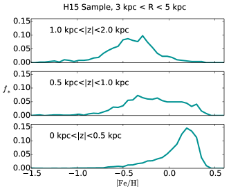
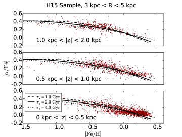
Figure 1.— (Top) MDFs of stars from the $3\,{\rm kpc}<R<5\,{\rm kpc}$ radial bin of H15, in three bins of $|z|$. [Fe/H] bins are of width 0.053 dex (75 bins over the range $-2.5<[{\rm Fe}/{\rm H}]<1.5$). In each panel, the MDF is normalized to the total number of stars in that layer. (Bottom) Distribution of the sample in $[\alpha/{\rm Fe}]-[{\rm Fe}/{\rm H}]$ space, with each point representing one star. The black lines, which are the same in each panel, show the evolutionary track predicted by our chemical evolution code for linear-exponential star-formation timescale $t_{\rm sf}=3.0\,{\rm Gyr}$, outflow mass loading $\eta=1.5$, and star formation efficiency timescales $\tau_{*}=1.0\,{\rm Gyr}$, $2.0\,{\rm Gyr}$, and $4.0\,{\rm Gyr}$.

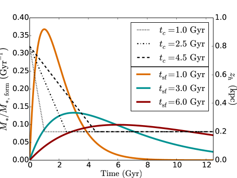
Figure 2.— Star formation rate and disk scale height as a function of time for our models. The colored curves show the fraction of stars formed in each timestep, as indicated by the left axis. These are normalized such that the area under each curve is 1.0, i.e. the cumulative number of stars is the same in each case after 12.5 Gyr has passed. The black lines indicate the scale-height of the disk over time and correspond to the right axis.

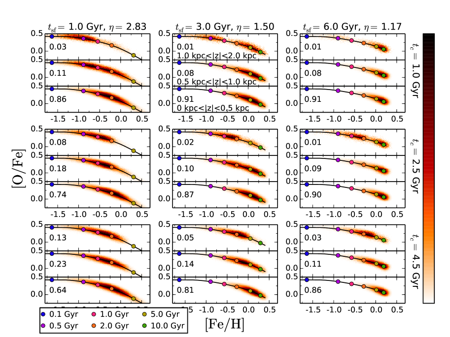
Figure 3.— Predictions of our nine models, plotted as 2D histograms in [O/Fe]-[Fe/H] space. Panels increase in $t_{\rm sf}$ from left to right and increase in $t_{c}$ from top to bottom. Each colored circle represents a timestamp corresponding to the times in the legend. Approximately $10^{6}$ stars are generated between 0.0 and 2.0 kpc in each model instance (the number is not exactly $10^{6}$ since a small number of stars form above 2.0 kpc); the fraction of these stars in each $|z|$-range are indicated on the lefthand side of each layer. There are 200 bins in the $x$-direction and 50 in the $y$-direction. The coloring is normalized such that white indicates 0 stars in a bin and black corresponds to the maximum number of stars in a bin within each layer, with a linear color scale shown on the right; thus, in the lower layers, where there are more stars, the color scale will cover a wider range of star counts than in the upper layers.

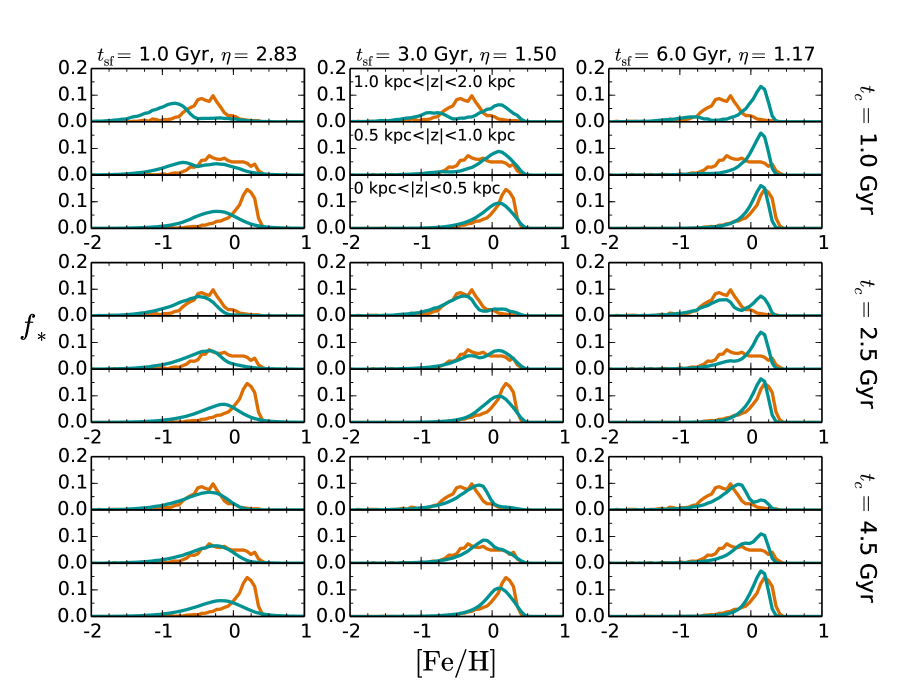
Figure 4.— MDFs in three $|z|$-layers for our nine models. The MDFs of the H15 stellar sample are plotted in orange. The blue curves show the model predictions. The panels increase in $t_{\rm sf}$ from left to right and increase in $t_{c}$ from top to bottom. MDFs are normalized separately in each layer, so that $f_{*}$ integrates to one in each sub-panel.

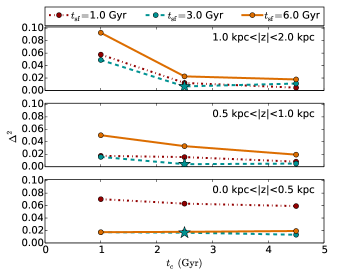
Figure 5.— The square difference (eq. 14) for the MDFs produced by each of our nine models in each $|z|$-layer. Lines connect models with the same value of $t_{\rm sf}$, while $t_{c}$ is indicated on the horizontal axis. The central model is marked with a star in each case.

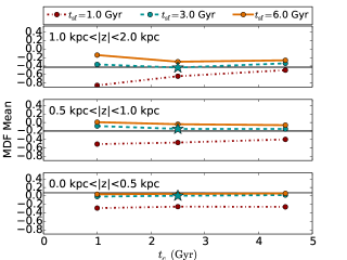
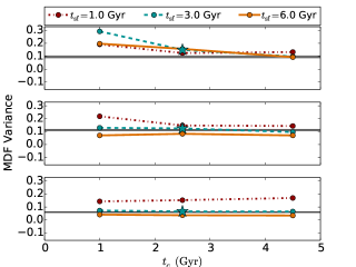
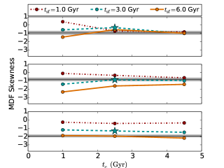
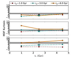
Figure 6.— Four statistical moments – mean, variance, skewness, and kurtosis (see Table 2) – for the MDFs produced by our nine models in each $|z|$-layer, and for the observed MDFs. Lines connect models with the same value of $t_{\rm sf}$, while $t_{c}$ is indicated on the horizontal axis. The central model is marked with a star in each case. The horizontal black line is the mean value of each statistic for the data, and the gray band denotes the 1-$\sigma$ error on this mean value as determined by bootstrap resampling of the dataset.

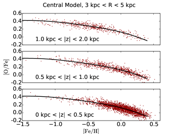
Figure 7.— The distribution of the H15 stellar sample in $[\alpha/{\rm Fe}]$-$[{\rm Fe}/{\rm H}]$ (top) compared to the predictions of our central model ($t_{\rm sf}=3.0\,{\rm Gyr}$, $t_{c}=2.5\,{\rm Gyr}$) on bottom. The stars generated by our model have been resampled to reflect the sampling of the data, such that the total number of stars in any given layer are approximately equal. Scatter of 0.05 dex in $[{\rm O}/{\rm Fe}]$ and $[{\rm Fe}/{\rm H}]$ is added to the model abundances.

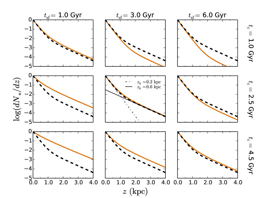
Figure 8.— Vertical distribution $dN_{*}/dz$ after 12.5 Gyr, normalized such that $\log(dN_{*}/dz)=0$ at $z=0$. Orange curves show the model predictions. Black dashed curves, the same in all panels for reference, show the sum of two exponentials with scale heights of $z_{h}=0.2\,{\rm kpc}$ and $0.6\,{\rm kpc}$, a decomposition that fits the predictions of our central model.

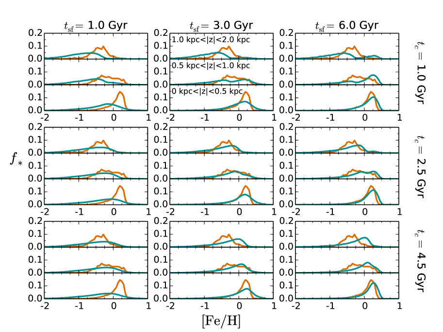
Figure 9.— MDFs for our nine models, in the case where star formation has an exponential form. Orange curves show the observed MDFs and blue curves show the model predictions. See the caption of Figure 4 for further explanation.

References

- Abadi et al. (2003) Abadi, M. G., Navarro, J. F., Steinmetz, M., & Eke, V. R. 2003, ApJ, 597, 21
- Alam et al. (2015) Alam, S., Albareti, F. D., Allende Prieto, C., et al. 2015, ApJS, 219, 12
- Andrews et al. (2016) Andrews, B. H., Weinberg, D. H., Schönrich, R., & Johnson, J. A. 2016, ArXiv e-prints
- Bensby et al. (2003) Bensby, T., Feltzing, S., & Lundström, I. 2003, A&A, 410, 527
- Bird et al. (2013) Bird, J. C., Kazantzidis, S., Weinberg, D. H., et al. 2013, ApJ, 773, 43
- Bournaud et al. (2009) Bournaud, F., Elmegreen, B. G., & Martig, M. 2009, ApJ, 707, L1
- Bovy et al. (2012) Bovy, J., Rix, H.-W., & Hogg, D. W. 2012, ApJ, 751, 131
- Bressan et al. (2012) Bressan, A., Marigo, P., Girardi, L., et al. 2012, MNRAS, 427, 127
- Brook et al. (2004) Brook, C. B., Kawata, D., Gibson, B. K., & Freeman, K. C. 2004, ApJ, 612, 894
- Chiappini et al. (1997) Chiappini, C., Matteucci, F., & Gratton, R. 1997, ApJ, 477, 765
- Chieffi & Limongi (2004) Chieffi, A., & Limongi, M. 2004, ApJ, 608, 405
- Davé et al. (2012) Davé, R., Finlator, K., & Oppenheimer, B. D. 2012, MNRAS, 421, 98
- De Silva et al. (2015) De Silva, G. M., Freeman, K. C., Bland-Hawthorn, J., et al. 2015, MNRAS, 449, 2604
- Edvardsson et al. (1993) Edvardsson, B., Andersen, J., Gustafsson, B., et al. 1993, A&A, 275, 101
- Eisenstein et al. (2011) Eisenstein, D. J., Weinberg, D. H., Agol, E., et al. 2011, AJ, 142, 72
- Finlator & Davé (2008) Finlator, K., & Davé, R. 2008, MNRAS, 385, 2181
- Forbes et al. (2012) Forbes, J., Krumholz, M., & Burkert, A. 2012, ApJ, 754, 48
- Forbes et al. (2014) Forbes, J. C., Krumholz, M. R., Burkert, A., & Dekel, A. 2014, MNRAS, 438, 1552
- García Pérez et al. (2016) García Pérez, A. E., Allende Prieto, C., Holtzman, J. A., et al. 2016, AJ, 151, 144
- Gilmore & Reid (1983) Gilmore, G., & Reid, N. 1983, MNRAS, 202, 1025
- Gilmore et al. (2012) Gilmore, G., Randich, S., Asplund, M., et al. 2012, The Messenger, 147, 25
- Hänninen & Flynn (2002) Hänninen, J., & Flynn, C. 2002, MNRAS, 337, 731
- Hayden et al. (2015) Hayden, M. R., Bovy, J., Holtzman, J. A., et al. 2015, ApJ, 808, 132
- Holtzman et al. (2015) Holtzman, J. A., Shetrone, M., Johnson, J. A., et al. 2015, AJ, 150, 148
- Iwamoto et al. (1999) Iwamoto, K., Brachwitz, F., Nomoto, K., et al. 1999, ApJS, 125, 439
- Jurić et al. (2008) Jurić, M., Ivezić, Ž., Brooks, A., et al. 2008, ApJ, 673, 864
- Kalirai et al. (2008) Kalirai, J. S., Hansen, B. M. S., Kelson, D. D., et al. 2008, ApJ, 676, 594
- Kroupa (2001) Kroupa, P. 2001, MNRAS, 322, 231
- Lee et al. (2011) Lee, Y. S., Beers, T. C., An, D., et al. 2011, ApJ, 738, 187
- Leroy et al. (2008) Leroy, A. K., Walter, F., Brinks, E., et al. 2008, AJ, 136, 2782
- Limongi & Chieffi (2006) Limongi, M., & Chieffi, A. 2006, ApJ, 647, 483
- Luo et al. (2015) Luo, A.-L., Zhao, Y.-H., Zhao, G., et al. 2015, Research in Astronomy and Astrophysics, 15, 1095
- Majewski et al. (2016) Majewski, S. R., Schiavon, R. P., Frinchaboy, P. M., et al. 2016, ArXiv e-prints
- Maoz et al. (2012) Maoz, D., Mannucci, F., & Brandt, T. D. 2012, MNRAS, 426, 3282
- Martig et al. (2016) Martig, M., Fouesneau, M., Rix, H.-W., et al. 2016, MNRAS, 456, 3655
- Ness et al. (2016) Ness, M., Hogg, D. W., Rix, H.-W., et al. 2016, ApJ, 823, 114
- Nidever et al. (2014) Nidever, D. L., Bovy, J., Bird, J. C., et al. 2014, ApJ, 796, 38
- Nidever et al. (2015) Nidever, D. L., Holtzman, J. A., Allende Prieto, C., et al. 2015, AJ, 150, 173
- Peeples & Shankar (2011) Peeples, M. S., & Shankar, F. 2011, MNRAS, 417, 2962
- Pinsonneault et al. (2014) Pinsonneault, M. H., Elsworth, Y., Epstein, C., et al. 2014, ApJS, 215, 19
- Schönrich & Binney (2009a) Schönrich, R., & Binney, J. 2009a, MNRAS, 396, 203
- Schönrich & Binney (2009b) —. 2009b, MNRAS, 399, 1145
- Sellwood & Binney (2002) Sellwood, J. A., & Binney, J. J. 2002, MNRAS, 336, 785
- Simha et al. (2014) Simha, V., Weinberg, D. H., Conroy, C., et al. 2014, ArXiv e-prints
- Stello et al. (2015) Stello, D., Huber, D., Sharma, S., et al. 2015, ApJ, 809, L3
- Talbot & Arnett (1971) Talbot, Jr., R. J., & Arnett, W. D. 1971, ApJ, 170, 409
- Tinsley (1980) Tinsley, B. M. 1980, Fund. Cosmic Phys., 5, 287
- Villalobos & Helmi (2008) Villalobos, Á., & Helmi, A. 2008, MNRAS, 391, 1806
- Vincenzo et al. (2016) Vincenzo, F., Matteucci, F., & Spitoni, E. 2016, ArXiv e-prints
- Weinberg et al. (2016) Weinberg, D. H., Andrews, B. H., & Freudenburg, J. 2016, ArXiv e-prints
- Wielen et al. (1996) Wielen, R., Fuchs, B., & Dettbarn, C. 1996, A&A, 314
- Zasowski et al. (2013) Zasowski, G., Johnson, J. A., Frinchaboy, P. M., et al. 2013, AJ, 146, 81