Scattering framework for two particles with isotropic spin-orbit coupling applicable to all energies

Abstract

Previous work developed a K-matrix formalism applicable to positive energies for the scattering between two $s$-wave interacting particles with two internal states, isotropic spin-orbit coupling and vanishing center-of-mass momentum [H. Duan, L. You and B. Gao, Phys. Rev A 87, 052708 (2013)]. This work extends the formalism to the entire energy regime. Explicit solutions are obtained for the total angular momentum $J=0$ and $1$ channels. The behavior of the partial cross sections in the negative energy regime is analyzed in detail. We find that the leading contributions to the partial cross sections at the negative energy thresholds are governed by the spin-orbit coupling strength $k_{\text{so}}$ and the mass ratio. The fact that these contributions are independent of the two-body scattering length $a_{s}$ is a direct consequence of the effective reduction of the dimensionality, and hence of the density of states, near the scattering thresholds due to the single-particle spin-orbit coupling terms. The results are analytically continued to the energy regime where bound states exist. It is shown that our results are consistent with results obtained by alternative approaches. Our formulation, which can be regarded as an extension of the standard textbook partial wave decomposition, can be generalized to two-body systems with other types of spin-orbit coupling, including cases where the center-of-mass momentum does not vanish.

I introduction

Spin-momentum coupling, which is associated with the presence of non-Abelian gauge fields, is crucial for a range of interesting effects in condensed matter physics. Throughout this article, we follow established terminology and refer to the coupling between a particle’s spin degrees of freedom and its canonical momentum as spin-orbit coupling condense_matter ; condense_matter1 . Some of the interest in these spin-orbit coupled systems stems from the fact that the single-particle dispersion curve displays Dirac rather than Schrödinger equation-type characteristics. The realization of synthetic gauge fields for neutral cold atom systems provides opportunities to (i) mimic condensed matter phenomena and (ii) look for novel physics not accessible with conventional condensed matter systems. In cold atom systems, a variety of techniques have been developed to create synthetic gauge fields, including lattice shaking sengstock and Raman coupling spielman . Raman laser coupling schemes have already led to the experimental realization of one-dimensional spin-orbit coupling (equal mixture of Rashba and Dresselhaus spin-orbit coupling) spielman ; zwierlein ; zhang ; pan and two-dimensional spin-orbit coupling 2D_SOC . This paper considers isotropic three-dimensional spin-orbit coupling. While this type of spin-orbit coupling has not yet been realized experimentally in cold atom systems, several proposals exist toward its experimental realization proposal_1 ; proposal_2 ; proposal_3 . The two-particle scattering framework developed in our work for systems with short-range interactions is related to scattering works for electronic systems with spin-orbit coupling. In the context of electronic systems, the negative energy regime, which is the focus of our work, has not received as much attention as the positive energy regime rashba_billiard ; Novikov ; Joel . Thus, we expect our developments to not only be of interest to the cold atom community but also to the condensed matter community.

Spin-orbit coupled cold atom systems are currently of great interest to experimentalists and theorists. To date a variety of exciting single-particle based phenomena such as Landau-Zener transitions landau_zener , Zitterbewegung oscillations Zitterbewegung , and spin wave dynamics spin_wave have been studied. Two-body interactions add a new degree of freedom to the system. For spin-orbit coupled systems, unlike in the alkalis, the singlet and triplet channels are strongly coupled, giving rise to changes of the two-body binding energy and the crossover physics in Fermi gases H_Hu ; ming_gong ; crossover_hui ; bound_shenoy ; crossover_shenoy ; rashbon_shenoy ; L_Han . While the experimental study of these effects is still in its infancy, first radio-frequency studies of weakly-bound Feshbach molecules reveal that the spin-orbit coupling terms have an appreciable effect zhang_jing . In a different experiment, the mixing of different partial waves was demonstrated explicitly in bosonic systems with one-dimensional spin-orbit coupling scattering_experiment . For a Bose-Einstein condensate, the existence of a stripe phase has been predicted theoretically based on the mean-field Gross-Pitaevskii equation. This new phase arises for certain Raman coupling strengths if the interspecies and intraspecies scattering lengths differ stripe_hui ; jason ; stripe ; stringari . The interplay between the two-body interactions and the single-particle spin-orbit coupling terms also leads to interesting few-body effects. For example, effectively one-dimensional systems with spin-orbit coupling allow for the realization of spin-chain models spin_chain_cui ; spin_chain_guan . Moreover, Borromean three-body states have been predicted to exist three_body_hui ; three_body_yi ; three_body_cui .

Motivated by the developments presented in Refs. Gao ; chris for positive energies, this paper develops a scattering formalism for two particles with isotropic spin-orbit coupling applicable to the entire energy regime. The formulation can be regarded as a generalization of the usual partial wave decomposition for two particles that are, at large interparticle distances, fully determined by the kinetic energy. In the presence of spin-orbit coupling, the particles’ behavior at large distances is governed by the combination of the kinetic energy and the spin-orbit coupling term. The presence of the spin-orbit coupling modifies the asymptotic form of the wave function to be matched to. Our formalism is illustrated for the contact $s$-wave interaction potential, which allows for the derivation of analytical expressions. While some of the results for the $(J,M_{J})=(0,0)$ channel had been derived previously bound_shenoy ; pengzhang ; pengzhang1 ; zhenhua ; xiaoling ; Gao , the results for the $(J,M_{J})=(1,M_{J})$ channel are, to the best of our knowledge, new. It is shown that the mass ratio can be used to tune the scattering properties. This finding suggests rich physics for unequal-mass systems with spin-orbit coupling. We find that the leading terms of the partial cross sections are independent of the $s$-wave scattering length for all negative energy scattering thresholds. This $s$-wave scattering length independence suggests a new type of universality, namely a regime where the two-body scattering cross sections are determined by the single-particle spin-orbit coupling parameter $k_{\text{so}}$. The effect can be traced back to an effective reduction of the dimensionality due to the spin-orbit coupling. While this effective dimensionality reduction is well known and appreciated bound_shenoy ; xiaoling ; review_hui , its impact on threshold laws has, to the best of our knowledge, not been discussed in detail in the literature. Our results for the $(J,M_{J})=(0,0)$ and $(1,M_{J})$ channels are related to results obtained by alternative approaches xiaoling ; pengzhang ; pengzhang1 ; zhenhua . It is demonstrated that the asymptotic basis chosen in our work and in Ref. xiaoling are different. With a proper unitary transformation, the solutions can, however, be transformed into each other (see also Ref. zhenhua ). While we, naturally, prefer our approach, it is argued that the use of the alternative asymptotic basis provides a useful complementary viewpoint. Last, our formulation provides the basis for numerical coupled-channel calculations for systems with spin-orbit coupling. While it was already pointed out in Ref. Gao that the partial wave decomposition approach only requires minor modifications of a typical coupled-channel code, it is our work that shows how to set such calculations up consistently over the entire energy regime.

The remainder of this paper is organized as follows. Section II introduces the general scattering framework. This framework is then applied to the $(J,M_{J})=(0,0)$ channel in Sec. III and to the $(J,M_{J})=(1,M_{J})$ channel in Sec. IV. Last, Sec. V provides a summary and an outlook.

II General formalism

For two particles interacting through a two-body short-range interaction potential $\hat{V}_{\text{2b}}(\mathbf{r}_{1}-\mathbf{r}_{2})$ with isotropic spin-orbit coupling terms that are proportional to $k_{\text{so}}$, the system Hamiltonian $\hat{H}_{\text{tot}}$ reads

$$\hat{H}_{\text{tot}} = \left(\frac{\hat{\mathbf{p}}_{1}^{2}}{2m_{1}}+\frac{\mathbf{\hat{p}}_{2}^{2}}{2m_{2}}\right)I_{1}\otimes I_{2}$$ (1)

$$+ \frac{\hbar k_{\text{so}}}{m_{1}}\left(\mathbf{\hat{p}}_{1}\cdot\hat{\boldsymbol{\sigma}}_{1}\right)\otimes I_{2}+\frac{\hbar k_{\text{so}}}{m_{2}}I_{1}\otimes\left(\mathbf{\hat{p}}_{2}\cdot\hat{\boldsymbol{\sigma}}_{2}\right)$$

$$+ \hat{V}_{\text{2b}}(\mathbf{r}_{1}-\mathbf{r}_{2})I_{1}\otimes I_{2}.$$

Here, $\mathbf{\hat{p}}_{j}$ denotes the canonical momentum operator of the $j$th particle, $m_{j}$ the mass of the $j$th particle, $\hat{\boldsymbol{\sigma}}_{j}$ a vector that contains the three Pauli matrices of the $j$th particle, and $\mathbf{r}_{j}$ the position vector of the $j$th particle. In Eq. (1), $I_{j}$ denotes the $2$ by $2$ identity matrix that spans the Hilbert space of the spin degrees of freedom of the $j$th particle. Defining the center-of-mass and relative coordinates $\mathbf{R}$ and $\mathbf{r}$, $\mathbf{R}=(m_{1}\mathbf{r}_{1}+m_{2}\mathbf{r}_{2})/(m_{1}+m_{2})$ and $\mathbf{r}=\mathbf{r}_{1}-\mathbf{r}_{2}$, Eq. (1) can be rewritten as

$$\hat{H}_{\text{tot}}=\hat{H}_{\text{com}}^{0}+\hat{H}_{\text{rel}}^{0}+\hat{V}_{\text{2b}}(\mathbf{r})I_{1}\otimes I_{2},$$ (2)

where

$$\hat{H}_{\text{com}}^{0}=\frac{\mathbf{\hat{P}}^{2}}{2M}I_{1}\otimes I_{2}+\frac{\hbar k_{\text{so}}}{M}\mathbf{\hat{P}}\cdot(\hat{\boldsymbol{\sigma}}_{1}\otimes I_{2}+I_{1}\otimes\hat{\boldsymbol{\sigma}}_{2})$$ (3)

and

$$\hat{H}_{\text{rel}}^{0} = \frac{\mathbf{\hat{p}}^{2}}{2\mu}I_{1}\otimes I_{2}$$ (4)

$$+ \frac{\hbar k_{\text{so}}}{\mu}\mathbf{\hat{p}}\cdot\left(\frac{m_{2}\hat{\boldsymbol{\sigma}}_{1}\otimes I_{2}-m_{1}I_{1}\otimes\hat{\boldsymbol{\sigma}}_{2}}{M}\right).$$

Here, $M$ and $\mu$ denote the center-of-mass and reduced masses, $M=m_{1}+m_{2}$ and $\mu=m_{1}m_{2}/(m_{1}+m_{2})$, and $\mathbf{\hat{P}}$ and $\mathbf{\hat{p}}$ are the center-of-mass and relative momentum operators, $\mathbf{\hat{P}}=\mathbf{\hat{p}}_{1}+\mathbf{\hat{p}}_{2}$ and $\mathbf{\hat{p}}=(m_{2}\mathbf{\hat{p}}_{1}-m_{1}\mathbf{\hat{p}}_{2})/M$. Since the system Hamiltonian $\hat{H}_{\text{tot}}$ commutes with $\mathbf{\hat{P}}$ comment_on_permute , the center-of-mass momentum is conserved. Throughout this paper, we consider the situation where the expectation value of the center-of-mass momentum vanishes. Integrating out the center-of-mass degrees of freedom, the Hamiltonian $\hat{H}_{\text{tot}}$ reduces to

$$\hat{H}=\hat{H}_{\text{rel}}^{0}+\hat{V}_{\text{2b}}(\mathbf{r})I_{1}\otimes I_{2}.$$ (5)

We start our discussion by considering the non-interacting Hamiltonian $\hat{H}_{\text{rel}}^{0}$. Defining

$$\hat{\boldsymbol{\Sigma}}=(m_{2}\hat{\boldsymbol{\sigma}}_{1}\otimes I_{2}-m_{1}I_{1}\otimes\hat{\boldsymbol{\sigma}}_{2})/M$$ (6)

and the relative helicity operator $\hat{h}_{\text{rel}}$,

$$\hat{h}_{\text{rel}}=\frac{\hat{\mathbf{p}}\cdot\hat{\boldsymbol{\Sigma}}}{|\langle\hat{\mathbf{p}}\cdot\hat{\boldsymbol{\Sigma}}\rangle|},$$ (7)

Eq. (4) can be rewritten as

$$\hat{H}_{\text{rel}}^{0}=\frac{\hat{\mathbf{p}}^{2}}{2\mu}I_{1}\otimes I_{2}+\frac{\hbar k_{\text{so}}}{\mu}\hat{h}_{\text{rel}}|\langle\hat{\mathbf{p}}\cdot\hat{\boldsymbol{\Sigma}}\rangle|.$$ (8)

The expectation value $|\langle\hat{\mathbf{p}}\cdot\hat{\mathbf{\Sigma}}\rangle|$ in the denominator of $\hat{h}_{\text{rel}}$, which serves as a “normalization factor”, is evaluated with respect to the same state as the expectation value of $\hat{H}_{\text{rel}}^{0}$. Since $\hat{h}_{\text{rel}}$ commutes with $\hat{H}_{\text{rel}}^{0}$, the eigenstates and eigenvalues of $\hat{H}_{\text{rel}}^{0}$ can be labeled by the eigenvalues $h_{\text{rel}}$ of $\hat{h}_{\text{rel}}$, where $h_{\text{rel}}$ can take the values $1$ and $-1$.

To determine the eigenenergies of $\hat{H}_{\text{rel}}^{0}$, we consider a fixed relative momentum quantum number $\mathbf{p}$ and define $\mathbf{p}=\hbar\mathbf{k}$ and $k=|\mathbf{k}|$. For a state with fixed $\mathbf{p}$ and $h_{\text{rel}}$, we have $|\langle\hat{\mathbf{p}}\cdot\hat{\boldsymbol{\Sigma}}\rangle|=\hbar k|\langle\hat{\boldsymbol{\Sigma}}\rangle|$ expectation_value_argument . Since $|\langle\hat{\boldsymbol{\Sigma}}\rangle|$ can take the values $1$ and $\eta$, where

$$\eta=(m_{2}-m_{1})/M,$$ (9)

the eigenenergies of $\hat{H}_{\text{rel}}^{0}$ are

$$E_{A}=\frac{\hbar^{2}(\bar{k}+k_{\text{so}})^{2}}{2\mu}-E_{r}$$ (10)

and

$$E_{B}=\frac{\hbar^{2}(\bar{k}+\eta k_{\text{so}})^{2}}{2\mu}-\eta^{2}E_{r}.$$ (11)

Here, $\bar{k}=h_{\text{rel}}k$ and $E_{r}$ is the recoil energy, $E_{r}=\hbar^{2}k_{\text{so}}^{2}/(2\mu)$. The energies $E_{A}$ and $E_{B}$ are referred to as the energies of branch A and branch B, respectively.

Figure 1(a) shows the eigenenergies of $\hat{H}_{\text{rel}}^{0}$ as a function of $k$ for equal masses (i.e., for $\eta=0$). These dispersion curves are shown in many papers, including those discussing two-body scattering xiaoling ; Gao . Since $k$ is by definition positive, only the positive side of the horizontal axis exists. The curves labeled by $\alpha$ and $\delta$ show $E_{A}$ and the curves labeled by $\beta$ and $\gamma$ show $E_{B}$; note that the curves labeled by $\beta$ and $\gamma$ are—for the equal-mass case shown—degenerate. In Fig. 1(a), the red and green solid lines show the energy of states with positive relative helicity ($h_{\text{rel}}=1$) while the circles and triangles show the energy of states with negative relative helicity ($h_{\text{rel}}=-1$). Figure 1(b) replots the eigenenergies as a function of $\bar{k}$. Since $\bar{k}=h_{\text{rel}}k$, the eigenenergies corresponding to states with negative helicity (symbols) are, compared to Fig. 1(a), “flipped” to negative $\bar{k}$. While there exist four states for a fixed $k$ in Fig. 1(a), there exist two states for a fixed $\bar{k}$ in Fig. 1(b). In this representation, branch A and branch B each correspond to smooth parabola.

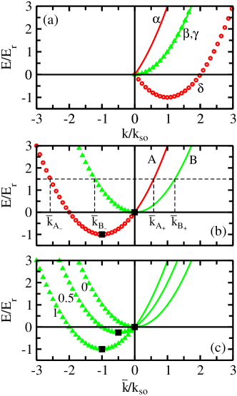
Figure 1: (Color online) Dispersion relationships for $\hat{H}_{\text{rel}}^{0}$. The energies $E_{A}$ (red solid lines and circles) and $E_{B}$ (green solid lines and triangles) are shown for $\eta=0$ as a function of $k$ in panel (a) and as a function of $\bar{k}$ in panel (b); the solid lines correspond to $h_{\text{rel}}=1$ and the symbols correspond to $h_{\text{rel}}=-1$. For a fixed positive energy [see the horizontal dashed line in panel (b)], there exist four real solutions for $\bar{k}$, denoted by $\bar{k}_{A_{+}}$, $\bar{k}_{A_{-}}$, $\bar{k}_{B_{+}}$, and $\bar{k}_{B_{-}}$ [see the vertical dashed lines and the discussion after Eq. (II)]; for $-E_{r}<E<0$, there exist only two real solutions for $\bar{k}$. Panel (c) shows the energy $E_{B}$ for $\eta=0,1/2$ and $1$ (see the labels in the figure). In panels (b) and (c), the filled squares show the minima $\bar{k}_{A}^{\text{min}}$ and $\bar{k}_{B}^{\text{min}}$.

Figure 1(c) illustrates the mass dependence of the energy of branch B. For a finite mass imbalance, the minimum of branch B is located at finite negative $\bar{k}$. Specifically, as $\eta$ increases from 0 to 1, the minimum $\bar{k}_{B}^{\text{min}}$ of $E_{B}$ moves from $0$ to $-k_{\text{so}}$. For $\eta=1$ (infinite mass imbalance), branch B is degenerate with branch A. Since branch $A$ is independent of $\eta$, the minimum $\bar{k}_{A}^{\text{min}}$ of $E_{A}$ does not move as $\eta$ changes. The minima $\bar{k}^{\text{min}}_{A}$ and $\bar{k}^{\text{min}}_{B}$ are shown by the filled black squares in Figs. 1(b) and 1(c).

To obtain the eigenstates of $\hat{H}_{\text{rel}}^{0}$, we write $\mathbf{k}$ in spherical coordinates, $\mathbf{k}=k\mathbf{n}$ with $k$ the magnitude of $\mathbf{k}$ and $\mathbf{n}$ the unit vector in the direction of $\mathbf{k}$, $\mathbf{n}=\left(\sin\theta_{\mathbf{k}}\cos\phi_{\mathbf{k}},\sin\theta_{\mathbf{k}}\sin\phi_{\mathbf{k}},\cos\theta_{\mathbf{k}}\right)$, and diagonalize the 4 by 4 Hamiltonian matrix in spin space. The resulting eigenstates of the branches labeled by $\alpha$, $\beta$, $\gamma$, and $\delta$ in Fig. 1(a) are

$$|\alpha\rangle^{+} = \frac{e^{\imath\mathbf{k}\cdot\mathbf{r}}}{(2\pi)^{3/2}}\Bigg{(}-\frac{1}{\sqrt{2}}e^{\imath\phi_{\mathbf{k}}}|\chi_{0,0}\rangle-\frac{\sin\theta_{\mathbf{k}}}{2}e^{2\imath\phi_{\mathbf{k}}}|\chi_{1,-1}\rangle$$ (12)

$$- \frac{\cos\theta_{\mathbf{k}}}{\sqrt{2}}e^{\imath\phi_{\mathbf{k}}}|\chi_{1,0}\rangle+\frac{\sin\theta_{\mathbf{k}}}{2}|\chi_{1,1}\rangle\Bigg{)},$$

$$|\delta\rangle^{-} = \frac{e^{\imath\mathbf{k}\cdot\mathbf{r}}}{(2\pi)^{3/2}}\Bigg{(}\frac{1}{\sqrt{2}}e^{\imath\phi_{\mathbf{k}}}|\chi_{0,0}\rangle-\frac{\sin\theta_{\mathbf{k}}}{2}e^{2\imath\phi_{\mathbf{k}}}|\chi_{1,-1}\rangle$$ (13)

$$- \frac{\cos\theta_{\mathbf{k}}}{\sqrt{2}}e^{\imath\phi_{\mathbf{k}}}|\chi_{1,0}\rangle+\frac{\sin\theta_{\mathbf{k}}}{2}|\chi_{1,1}\rangle\Bigg{)},$$

$$|\beta\rangle^{+} = \frac{e^{\imath\mathbf{k}\cdot\mathbf{r}}}{(2\pi)^{3/2}}\Bigg{[}\sin^{2}\left(\frac{\theta_{\mathbf{k}}}{2}\right)e^{2\imath\phi_{\mathbf{k}}}|\chi_{1,-1}\rangle$$ (14)

$$+ \frac{\sin\theta_{\mathbf{k}}}{\sqrt{2}}e^{\imath\phi_{\mathbf{k}}}|\chi_{1,0}\rangle+\cos^{2}\left(\frac{\theta_{\mathbf{k}}}{2}\right)|\chi_{1,1}\rangle\Bigg{]},$$

and

$$|\gamma\rangle^{-} = \frac{e^{\imath\mathbf{k}\cdot\mathbf{r}}}{(2\pi)^{3/2}}\Bigg{[}\cos^{2}\left(\frac{\theta_{\mathbf{k}}}{2}\right)e^{2\imath\phi_{\mathbf{k}}}|\chi_{1,-1}\rangle$$ (15)

$$- \frac{\sin\theta_{\mathbf{k}}}{\sqrt{2}}e^{\imath\phi_{\mathbf{k}}}|\chi_{1,0}\rangle+\sin^{2}\left(\frac{\theta_{\mathbf{k}}}{2}\right)|\chi_{1,1}\rangle\Bigg{]}.$$

Here, the superscripts “$+$” and “$-$” indicate the relative helicity (“$+$” corresponds to $h_{\text{rel}}=1$ and “$-$” to $h_{\text{rel}}=-1$). Our goal is now to combine the states $|\alpha\rangle^{+}$ and $|\delta\rangle^{-}$ into a single state, the eigenstate $|\bar{k},\theta_{\mathbf{k}},\phi_{\mathbf{k}}\rangle_{A}$ of branch A. Inspection of Eqs. (12) and (13) shows that the spatial parts are not changing smoothly when the relative helicity changes from “$+$” to “$-$” (the spatial part associated with $|\chi_{0,0}\rangle$ changes sign). Since the eigenstate $|\delta\rangle^{-}$ depends parametrically on $\mathbf{k}$, the state given in Eq. (13) remains an eigenstate if we change $\mathbf{k}$ to $-\mathbf{k}$. Making this replacement and using the identities $\theta_{-\mathbf{k}}=\pi-\theta_{\mathbf{k}}$ and $\phi_{-\mathbf{k}}=\pi+\phi_{\mathbf{k}}$, Eq. (13) becomes

$$|\delta\rangle^{-} = \frac{e^{-\imath\mathbf{k}\cdot\mathbf{r}}}{(2\pi)^{3/2}}\Bigg{(}-\frac{1}{\sqrt{2}}e^{\imath\phi_{\mathbf{k}}}|\chi_{0,0}\rangle-\frac{\sin\theta_{\mathbf{k}}}{2}e^{2\imath\phi_{\mathbf{k}}}|\chi_{1,-1}\rangle$$ (16)

$$- \frac{\cos\theta_{\mathbf{k}}}{\sqrt{2}}e^{\imath\phi_{\mathbf{k}}}|\chi_{1,0}\rangle+\frac{\sin\theta_{\mathbf{k}}}{2}|\chi_{1,1}\rangle\Bigg{)}.$$

Using $\bar{k}=h_{\text{rel}}k$, Eqs. (12) and (16) can be combined to yield the eigenstate $|\bar{k},\theta_{\mathbf{k}},\phi_{\mathbf{k}}\rangle_{A}$ of branch A,

$$|\bar{k},\theta_{\mathbf{k}},\phi_{\mathbf{k}}\rangle_{A} = \frac{e^{\imath\bar{k}\mathbf{n}\cdot\mathbf{r}}}{(2\pi)^{3/2}}\times$$ (17)

$$\Bigg{(}-\frac{1}{\sqrt{2}}e^{\imath\phi_{\mathbf{k}}}|\chi_{0,0}\rangle-\frac{\sin\theta_{\mathbf{k}}}{2}e^{2\imath\phi_{\mathbf{k}}}|\chi_{1,-1}\rangle$$

$$-\frac{\cos\theta_{\mathbf{k}}}{\sqrt{2}}e^{\imath\phi_{\mathbf{k}}}|\chi_{1,0}\rangle+\frac{\sin\theta_{\mathbf{k}}}{2}|\chi_{1,1}\rangle\Bigg{)}.$$

For a fixed $\mathbf{n}$, the branch A state changes smoothly from a state with “$+$” relative helicity to a state with “$-$” relative helicity if the quantity $\bar{k}$ goes through zero. The state has positive relative helicity if $\bar{k}\mathbf{n}$ is parallel to $\langle\hat{\mathbf{\Sigma}}\rangle$ and negative relative helicity if $\bar{k}\mathbf{n}$ is anti-parallel to $\langle\hat{\mathbf{\Sigma}}\rangle$. The eigenstate $|\bar{k},\theta_{\mathbf{k}},\phi_{\mathbf{k}}\rangle_{B}$ of branch B with energy $E_{B}$ can be obtained by applying an analogous logic to Eqs. (14) and (15). We find

$$|\bar{k},\theta_{\mathbf{k}},\phi_{\mathbf{k}}\rangle_{B} =\frac{e^{\imath\bar{k}\mathbf{n}\cdot\mathbf{r}}}{(2\pi)^{3/2}}\Bigg{[}\sin^{2}\left(\frac{\theta_{\mathbf{k}}}{2}\right)e^{2\imath\phi_{\mathbf{k}}}|\chi_{1,-1}\rangle+$$ (18)

$$\frac{\sin\theta_{\mathbf{k}}}{\sqrt{2}}e^{\imath\phi_{\mathbf{k}}}|\chi_{1,0}\rangle+\cos^{2}\left(\frac{\theta_{\mathbf{k}}}{2}\right)|\chi_{1,1}\rangle\Bigg{]}.$$

The expectation value of $\hat{h}_{\text{rel}}$ with respect to $|\bar{k},\theta_{\mathbf{k}},\phi_{\mathbf{k}}\rangle_{A}$ and $|\bar{k},\theta_{\mathbf{k}},\phi_{\mathbf{k}}\rangle_{B}$ is $\bar{k}/|\bar{k}|$, which equals $+1$ for $\bar{k}>0$ (positive helicity) and $-1$ for $\bar{k}<0$ (negative helicity).

We now construct, following the logic of Refs. Gao ; chris , the eigenstates of $\hat{H}_{\text{rel}}^{0}$ with good total angular momentum quantum number $J$ and corresponding projection quantum number $M_{J}$. $\hat{H}_{\text{rel}}^{0}$ commutes with the square of the total angular momentum operator $\hat{\mathbf{J}}$ and its $z$-component $\hat{J}_{z}$, where $\hat{\mathbf{J}}^{2}=(\hat{\mathbf{L}}+\hat{\mathbf{S}})^{2}$ and $\hat{J}_{z}=\hat{L}_{z}+\hat{S}_{z}$. Here, $\hat{\mathbf{L}}$ is the relative orbital angular momentum operator of the two-particle system. Using standard angular momentum algebra zare , the eigenstates of $\hat{\mathbf{J}}^{2}$ and $\hat{J}_{z}$ are constructed by taking linear combinations of states with different orbital angular momentum and spin angular momentum quantum numbers,

$$|J,M_{J};L,S\rangle=\sum_{M_{L},M_{S}}c_{M_{L},M_{S}}^{J,M_{J},L,S}|L,M_{L};S,M_{S}\rangle,$$ (19)

where the $c_{M_{L},M_{S}}^{J,M_{J},L,S}$ denote Clebsch-Gordan coefficients and $M_{L}$ and $M_{S}$ the projection quantum numbers corresponding to the operators $\hat{L}_{z}$ and $\hat{S}_{z}$, respectively. For each $(J,M_{J})$ channel, we expand the eigenstates $\psi^{(J,M_{J})}(\bar{k}\mathbf{r})$ of $\hat{H}_{\text{rel}}^{0}$ into components labeled by $(J,M_{J};L,S)$,

$$\psi^{(J,M_{J})}(\bar{k}\mathbf{r})=\sum_{L,S}\frac{u_{L,S}^{(J,M_{J})}(\bar{k}r)}{r}|J,M_{J};L,S\rangle,$$ (20)

where the sums over $L$ and $S$ go over all quantum numbers allowed by angular momentum coupling and where the “weights” $u^{(J,M_{J})}_{L,S}(\bar{k}r)/r$ have the unit of inverse length and depend on the distance $r$. To obtain the weights for $\psi^{(J,M_{J})}(\bar{k}\mathbf{r})$ (assuming that $J$ and $M_{J}$ are fixed), we project the plane wave solutions, Eqs. (17)-(18), onto each $(J,M_{J};L,S)$ component. This projection yields the following general structure for $\psi^{(J,M_{J})}(\bar{k}\mathbf{r})$,

$$\psi_{\text{reg}}^{(J,M_{J})}(\bar{k}\mathbf{r})=\sum_{L,S}a_{L,S}^{J,M_{J}}\bar{k}j_{L}(\bar{k}r)|J,M_{J};L,S\rangle,$$ (21)

where $j_{L}(\bar{k}r)$ is the spherical Bessel function of order $L$. Here, the coefficients $a_{L,S}^{J,M_{J}}$ are normalized such that $\sum_{L,S}|a_{L,S}^{J,M_{J}}|^{2}=1$. Equation (21) constitutes the regular eigenstates of $\hat{H}_{\text{rel}}^{0}$. To span the full Hilbert space, a set of irregular solutions is needed in addition to the regular solutions. Replacing the spherical Bessel functions $j_{L}(\bar{k}r)$ in Eq. (21) by spherical Neumann functions $n_{L}(\bar{k}r)$, we obtain the irregular solutions

$$\psi_{\text{irr}}^{(J,M_{J})}(\bar{k}\mathbf{r})=\sum_{L,S}a_{L,S}^{J,M_{J}}\bar{k}n_{L}(\bar{k}r)|J,M_{J};L,S\rangle.$$ (22)

Looking ahead, we define

$$\underline{$\psi$}_{\text{reg}}^{(J,M_{J})}(\bar{k}r)=\left(a_{L_{1},S_{1}}^{J,M_{J}}\bar{k}j_{L_{1}}(\bar{k}r),a_{L_{2},S_{2}}^{J,M_{J}}\bar{k}j_{L_{2}}(\bar{k}r),...\right)^{T}$$ (23)

and

$$\underline{$\psi$}_{\text{irr}}^{(J,M_{J})}(\bar{k}r)=\left(a_{L_{1},S_{1}}^{J,M_{J}}\bar{k}n_{L_{1}}(\bar{k}r),a_{L_{2},S_{2}}^{J,M_{J}}\bar{k}n_{L_{2}}(\bar{k}r),...\right)^{T}.$$ (24)

We now consider a non-vanishing short-range potential $\hat{V}_{\text{2b}}(\mathbf{r})$. For a spherically symmetric two-body interaction potential $\hat{V}_{\text{2b}}(\mathbf{r})$, the Hamiltonian $\hat{H}$, Eq. (5), commutes with $\hat{\mathbf{J}}^{2}$ and $\hat{J}_{z}$. Thus we seek scattering solutions for each $(J,M_{J})$ channel. The radial scattering wave function $\Psi^{(J,M_{J})}(r)$ in the $(J,M_{J})$ channel for a fixed energy is written asymptotically, in the large $r$ limit, as

$$\Psi^{(J,M_{J})}(r)\xrightarrow{r\to\infty}\mathcal{J}^{(J,M_{J})}(r)-\mathcal{N}^{(J,M_{J})}(r)\mathcal{K}^{(J,M_{J})},$$ (25)

where

$$\mathcal{J}^{(J,M_{J})}(r)=$$

$$\Big{[} N_{A_{+}}\underline{$\psi$}_{\text{reg}_{A}}^{(J,M_{J})}(\bar{k}_{A_{+}}r),N_{A_{-}}\underline{$\psi$}_{\text{reg}_{A}}^{(J,M_{J})}(\bar{k}_{A_{-}}r),$$

$$N_{B_{+}}\underline{$\psi$}_{\text{reg}_{B}}^{(J,M_{J})}(\bar{k}_{B_{+}}r),N_{B_{-}}\underline{$\psi$}_{\text{reg}_{B}}^{(J,M_{J})}(\bar{k}_{B_{-}}r)\Big{]}$$ (26)

and

$$\mathcal{N}^{(J,M_{J})}(r)=$$

$$\Big{[} N_{A_{+}}\underline{$\psi$}_{\text{irr}_{A}}^{(J,M_{J})}(\bar{k}_{A+}r),-N_{A_{-}}\underline{$\psi$}_{\text{irr}_{A}}^{(J,M_{J})}(\bar{k}_{A-}r),$$

$$N_{B_{+}}\underline{$\psi$}_{\text{irr}_{B}}^{(J,M_{J})}(\bar{k}_{B+}r),-N_{B_{-}}\underline{$\psi$}_{\text{irr}_{B}}^{(J,M_{J})}(\bar{k}_{B-}r)\Big{]}.$$ (27)

Here, the subscripts $A$ and $B$ are added to the wave functions $\underline{$\psi$}_{\text{reg}}^{(J,M_{J})}(\bar{k}r)$ and $\underline{$\psi$}_{\text{irr}}^{(J,M_{J})}(\bar{k}r)$, Eqs. (23) and (24), to indicate the regular and irregular solutions of branch A and branch B, respectively. The subscripts $A_{+}$ and $A_{-}$ distinguish the two allowed $\bar{k}$ of branch A at fixed energy. We use the convention $\bar{k}_{A_{+}}>\bar{k}_{A}^{\text{min}}$ and $\bar{k}_{A_{-}}<\bar{k}_{A}^{\text{min}}$. Similarly, the subscripts $B_{+}$ and $B_{-}$ distinguish the two allowed $\bar{k}$ of branch B at fixed energy. We use the convention $\bar{k}_{B_{+}}>\bar{k}_{B}^{\text{min}}$ and $\bar{k}_{B_{-}}<\bar{k}_{B}^{\text{min}}$ [see Fig. 1(b) for an illustration]. The $N_{A_{+}}$, $N_{A_{-}}$, $N_{B_{+}}$, and $N_{B_{-}}$ denote current normalization factors that are chosen such that the flux over a closed surface encircling the origin for a state with outgoing current is normalized to $1$ [see Eqs. (35) and (36) below and Ref. note_on_normalization ]. The forms of $\mathcal{J}^{(J,M_{J})}(r)$ and $\mathcal{N}^{(J,M_{J})}(r)$ in Eqs. (II) and (II) ensure that the scattering matrix $\mathcal{S}^{(J,M_{J})}$ is related to the reaction matrix $\mathcal{K}^{(J,M_{J})}$ in the “usual way” when the outgoing current boundary condition at large $r$ is matched (see the discussion below), namely through

$$\mathcal{S}^{(J,M_{J})}=(I+\imath\mathcal{K}^{(J,M_{J})})(I-\imath\mathcal{K}^{(J,M_{J})})^{-1}.$$ (28)

Here, $I$ denotes the identity matrix. The reaction matrix $\mathcal{K}^{(J,M_{J})}$ is determined by matching the radial wave functions to the asymptotic form, Eq. (25), at sufficiently large interparticle distances. Specifically, if we know the large $r$ behavior of the wave function $\Psi^{(J,M_{J})}(r)$ in the $|J,M_{J};L,S\rangle$ basis for a short-range interaction potential $\hat{V}_{\text{2b}}(\mathbf{r})$, then we can match its asymptotic large $r$ behavior to Eq. (25). In general, $\Psi^{(J,M_{J})}(r)$ can be obtained by propagating the logarithmic derivative matrix using an appropriate propagation scheme. Importantly, since Eqs. (II) and (II) are continuous with respect to the arguments $\bar{k}_{A_{+}},\bar{k}_{A_{-}},\bar{k}_{B_{+}}$, and $\bar{k}_{B_{-}}$ and since these arguments change smoothly when the energy goes from small positive to small negative values, $\Psi^{(J,M_{J})}(r)$ changes smoothly as the energy goes from positive to negative values.

To relate the scattering matrix $\mathcal{S}^{(J,M_{J})}$ and the reaction matrix $\mathcal{K}^{(J,M_{J})}$, we analyze the outgoing currents at large distances. The relative current $\mathbf{j}(\mathbf{r})$ for state $\psi^{(J,M_{J})}(\bar{k}\mathbf{r})$ is defined through

$$\mathbf{j}(\mathbf{r})=\frac{1}{2\mu}\Bigg{\{}(\psi^{(J,M_{J})})^{\dagger}\mathbf{p}_{k}\psi^{(J,M_{J})}+$$

$$\left[(\psi^{(J,M_{J})})^{\dagger}\mathbf{p}_{k}\psi^{(J,M_{J})}\right]^{*}\Bigg{\}},$$ (29)

where $\mathbf{p}_{k}$ is the relative kinetic momentum operator, which is related to the relative canonical momentum operator $\mathbf{p}$ by $\mathbf{p}_{k}=\mu[\mathbf{r},H_{\text{rel}}^{0}]/(\imath\hbar)$. We find

$$\mathbf{p}_{k}=\mathbf{p}I_{1}\otimes I_{2}+\hbar k_{\text{so}}\hat{\boldsymbol{\Sigma}}.$$ (30)

Recall, $\psi^{(J,M_{J})}$ is a four-component spinor and each of the three components of $\mathbf{p}_{k}$ is a $4$ by $4$ matrix. Doing the multiplications in Eq. (II), we can check that $\mathbf{j}(\mathbf{r})$ is—as it should be—a three-component vector. To obtain scattering wave functions that correspond to outgoing current at large $r$, we consider the following two linear combinations of Eqs. (21) and (22),

$$\psi^{(J,M_{J})+}(\bar{k}\mathbf{r})=\imath\psi_{\text{reg}}^{(J,M_{J})}(\bar{k}\mathbf{r})-\psi_{\text{irr}}^{(J,M_{J})}(\bar{k}\mathbf{r})$$ (31)

and

$$\psi^{(J,M_{J})-}(\bar{k}\mathbf{r})=-\imath\psi_{\text{reg}}^{(J,M_{J})}(\bar{k}\mathbf{r})-\psi_{\text{irr}}^{(J,M_{J})}(\bar{k}\mathbf{r}).$$ (32)

Here, $\psi^{(J,M_{J})+}(\bar{k}\mathbf{r})$ contains the “phase factor” $\text{e}^{\imath\bar{k}r}$ while $\psi^{(J,M_{J})-}(\bar{k}\mathbf{r})$ contains the “phase factor” $\text{e}^{-\imath\bar{k}r}$. The currents for $\psi^{(J,M_{J})+}(\bar{k}\mathbf{r})$ and $\psi^{(J,M_{J})-}(\bar{k}\mathbf{r})$ are

$$\mathbf{j}^{+}(\mathbf{r})=\frac{\hbar}{4\pi\mu r^{2}}(\bar{k}-\bar{k}^{\text{min}})\hat{\mathbf{r}}$$ (33)

and

$$\mathbf{j}^{-}(\mathbf{r})=-\frac{\hbar}{4\pi\mu r^{2}}(\bar{k}-\bar{k}^{\text{min}})\hat{\mathbf{r}},$$ (34)

respectively, where $\bar{k}^{\text{min}}$ is the $\bar{k}$ value at which the energy is minimal and $\hat{\mathbf{r}}$ is the unit vector in the $\mathbf{r}$ direction. Importantly, the states with outgoing current are $\psi^{(J,M_{J})+}(\bar{k}\mathbf{r})$ for $\bar{k}>\bar{k}^{\text{min}}$ and $\psi^{(J,M_{J})-}(\bar{k}\mathbf{r})$ for $\bar{k}<\bar{k}^{\text{min}}$. The current normalization factors are determined by enforcing current conservation, i.e., by enforcing

$$|N|^{2}\oint\mathbf{j}^{+}(\mathbf{r})\cdot\text{d}\mathbf{S}=1\text{ for }\ \bar{k}>\bar{k}^{\text{min}}$$ (35)

and

$$|N|^{2}\oint\mathbf{j}^{-}(\mathbf{r})\cdot\text{d}\mathbf{S}=1\text{ for }\ \bar{k}<\bar{k}^{\text{min}}.$$ (36)

Table 1 shows the current and the corresponding current normalization factor for the states $\psi_{A}^{(J,M_{J})+}$, $\psi_{A}^{(J,M_{J})-}$, $\psi_{B}^{(J,M_{J})+}$, and $\psi_{B}^{(J,M_{J})-}$.

state	$\mathbf{j}(\mathbf{r})$	$N$
$\psi_{A}^{(J,M_{J})+}(\bar{k}_{A_{+}}\mathbf{r})$	$+\frac{\hbar}{4\pi\mu r^{2}}(\bar{k}_{A_{+}}-\bar{k}_{A}^{\text{min}})\hat{\mathbf{r}}$, out	$\sqrt{{\mu}/[{\hbar(\bar{k}_{A_{+}}-\bar{k}_{A}^{\text{min}})}]}$
$\psi_{A}^{(J,M_{J})-}(\bar{k}_{A_{+}}\mathbf{r})$	$-\frac{\hbar}{4\pi\mu r^{2}}(\bar{k}_{A_{+}}-\bar{k}_{A}^{\text{min}})\hat{\mathbf{r}}$, in
$\psi_{A}^{(J,M_{J})+}(\bar{k}_{A_{-}}\mathbf{r})$	$+\frac{\hbar}{4\pi\mu r^{2}}(\bar{k}_{A_{-}}-\bar{k}_{A}^{\text{min}})\hat{\mathbf{r}}$, in	$\sqrt{{\mu}{/[-\hbar(\bar{k}_{A_{-}}-\bar{k}_{A}^{\text{min}})]}}$
$\psi_{A}^{(J,M_{J})-}(\bar{k}_{A_{-}}\mathbf{r})$	$-\frac{\hbar}{4\pi\mu r^{2}}(\bar{k}_{A_{-}}-\bar{k}_{A}^{\text{min}})\hat{\mathbf{r}}$, out
$\psi_{B}^{(J,M_{J})+}(\bar{k}_{B_{+}}\mathbf{r})$	$+\frac{\hbar}{4\pi\mu r^{2}}(\bar{k}_{B_{+}}-\bar{k}_{B}^{\text{min}})\hat{\mathbf{r}}$, out	$\sqrt{{\mu}{/[\hbar(\bar{k}_{B_{+}}-\bar{k}_{B}^{\text{min}})]}}$
$\psi_{B}^{(J,M_{J})-}(\bar{k}_{B_{+}}\mathbf{r})$	$-\frac{\hbar}{4\pi\mu r^{2}}(\bar{k}_{B_{+}}-\bar{k}_{B}^{\text{min}})\hat{\mathbf{r}}$, in
$\psi_{B}^{(J,M_{J})+}(\bar{k}_{B_{-}}\mathbf{r})$	$+\frac{\hbar}{4\pi\mu r^{2}}(\bar{k}_{B_{-}}-\bar{k}_{B}^{\text{min}})\hat{\mathbf{r}}$, in	$\sqrt{{\mu}{/[-\hbar(\bar{k}_{B_{-}}-\bar{k}_{B}^{\text{min}})]}}$
$\psi_{B}^{(J,M_{J})-}(\bar{k}_{B_{-}}\mathbf{r})$	$-\frac{\hbar}{4\pi\mu r^{2}}(\bar{k}_{B_{-}}-\bar{k}_{B}^{\text{min}})\hat{\mathbf{r}}$, out

Table 1: Columns 2 and 3 report, respectively, the current and the corresponding current normalization factor for the states listed in column 1. The labels “out” and “in” in column 2 indicate that the current points in the $+\hat{\mathbf{r}}$ and $-\hat{\mathbf{r}}$ direction, respectively. From top to bottom, the entries in column 3 correspond to $N_{A_{+}}$, $N_{A_{-}}$, $N_{B_{+}}$, and $N_{B_{-}}$.

For each branch A state, $\bar{k}$ takes the values $\bar{k}_{A_{+}}$ and $\bar{k}_{A_{-}}$; similarly, for each branch B state, $\bar{k}$ takes the values $\bar{k}_{B_{+}}$ and $\bar{k}_{B_{-}}$. Since we have $\bar{k}_{A_{+}}>\bar{k}_{A}^{\text{min}}$, $\bar{k}_{A_{-}}<\bar{k}_{A}^{\text{min}}$, $\bar{k}_{B_{+}}>\bar{k}_{B}^{\text{min}}$, and $\bar{k}_{B_{-}}<\bar{k}_{B}^{\text{min}}$, the current points in the $+\hat{\mathbf{r}}$ direction for the states $\psi_{A}^{(J,M_{J})+}(\bar{k}_{A_{+}}\mathbf{r})$, $\psi_{A}^{(J,M_{J})-}(\bar{k}_{A_{-}}\mathbf{r})$, $\psi_{B}^{(J,M_{J})+}(\bar{k}_{B_{+}}\mathbf{r})$, and $\psi_{B}^{(J,M_{J})-}(\bar{k}_{B_{-}}\mathbf{r})$; for the other four states, the current points in the $-\hat{\mathbf{r}}$ direction.

To obtain the scattering matrix $\mathcal{S}^{(J,M_{J})}$, we rewrite Eq. (25) in terms of the states listed in the first column of Table 1. Grouping the states with outgoing current together and those with incoming current together, we find

$$\Psi^{(J,M_{J})}(\bar{k}r)\xrightarrow{r\to\infty}$$

$$\frac{1}{2\imath}\Big{\{}\Big{[}N_{A_{+}}\underline{$\psi$}_{A}^{(J,M_{J})+}(\bar{k}_{A_{+}}r),-N_{A_{-}}\underline{$\psi$}_{A}^{(J,M_{J})-}(\bar{k}_{A_{-}}r),N_{B_{+}}\underline{$\psi$}_{B}^{(J,M_{J})+}(\bar{k}_{B_{+}}r),-N_{B_{-}}\underline{$\psi$}_{B}^{(J,M_{J})-}(\bar{k}_{B_{-}}r)\Big{]}\mathcal{S}^{(J,M_{J})}-$$

$$\Big{[}N_{A_{+}}\underline{$\psi$}_{A}^{(J,M_{J})-}(\bar{k}_{A+}r),-N_{A_{-}}\underline{$\psi$}_{A}^{(J,M_{J})+}(\bar{k}_{A-}r),N_{B_{+}}\underline{$\psi$}_{B}^{(J,M_{J})-}(\bar{k}_{B+}r),-N_{B_{-}}\underline{$\psi$}_{B}^{(J,M_{J})+}(\bar{k}_{B-}r)\Big{]}\Big{\}}(I-\imath\mathcal{K}^{(J,M_{J})}).$$ (37)

Important observables are the partial cross sections $\sigma_{jl}^{(J,M_{J})}$ that characterize the scattering from state $j$ to state $l$. Throughout this paper, state $j$ ($j=1-4$) corresponds to the state in the $j$th column of $\mathcal{J}^{(J,M_{J})}(r)$ and $\mathcal{N}^{(J,M_{J})}(r)$. This means that states 1-4 have the arguments $\bar{k}_{1}=\bar{k}_{A_{+}}$, $\bar{k}_{2}=\bar{k}_{A_{-}}$, $\bar{k}_{3}=\bar{k}_{B_{+}}$, and $\bar{k}_{4}=\bar{k}_{B_{-}}$. The partial cross sections partial_cross_section_argument are related to the elements of the $\mathcal{S}^{(J,M_{J})}$ matrix by

$$\sigma_{jl}^{(J,M_{J})}=\frac{2\pi}{\bar{k}_{j}^{2}}|\mathcal{S}_{lj}^{(J,M_{J})}-\delta_{jl}|^{2},$$ (38)

where $\delta_{jl}$ is the Kronecker delta function. Since the lowest scattering threshold occurs at $E=-E_{r}$, two-body bound states may exist for $E<-E_{r}$. The bound state energies can be obtained by analyzing the poles of the $\mathcal{S}^{(J,M_{J})}$ matrix. Explicit calculations for the $(J,M_{J})=(0,0)$ and $(1,M_{J})$ channels are detailed in the next two sections.

III $(J,M_{J})=(0,0)$ channel

This section considers the $(J,M_{J})=(0,0)$ channel. Angular momentum algebra yields that the components $(J,M_{J};L,S)=(0,0;0,0)$ and $(0,0;1,1)$ contribute. Since the $(J,M_{J};L,S)=(0,0;0,0)$ component contains the spherical harmonic $Y_{0,0}$, multiplied by the spin singlet, and since the $(J,M_{J};L,S)=(0,0;1,1)$ component contains the spherical harmonics $Y_{1,M_{L}}$ ($M_{L}=-1,0$, and $1$), multiplied by spin triplets, both components are anti-symmetric under the exchange of the two particles. Using the projection procedure outlined in the previous section, we find that branch $A$ has non-zero components in the $(J,M_{J})=(0,0)$ channel and that the last two columns in Eqs. (II) and (II) are zero. Thus, throughout this section, we drop the last two columns, i.e., we work with ${\cal{K}}^{(0,0)}$ and ${\cal{S}}^{(0,0)}$ matrices of size 2 by 2 that describe the physics of branch A. Since the dispersion relationship of branch $A$ is independent of the mass ratio, our results in this section are independent of the mass ratio. Thus, since both contributing components are anti-symmetric under the exchange of the two particles, the scattering solutions obtained in this section apply to either two identical fermions or to two distinguishable particles with equal or unequal masses. We have

$$\mathcal{J}^{(0,0)}(r)=$$

$$\begin{bmatrix}\frac{1}{\sqrt{2}}N_{A_{+}}\bar{k}_{A_{+}}j_{0}(\bar{k}_{A_{+}}r)&\frac{1}{\sqrt{2}}N_{A_{-}}\bar{k}_{A_{-}}j_{0}(\bar{k}_{A_{-}}r)\\ -\frac{\imath}{\sqrt{2}}N_{A_{+}}\bar{k}_{A_{+}}j_{1}(\bar{k}_{A_{+}}r)&-\frac{\imath}{\sqrt{2}}N_{A_{-}}\bar{k}_{A_{-}}j_{1}(\bar{k}_{A_{-}}r)\end{bmatrix},$$ (39)

$$\mathcal{N}^{(0,0)}(r)=$$

$$\begin{bmatrix}\frac{1}{\sqrt{2}}N_{A_{+}}\bar{k}_{A_{+}}n_{0}(\bar{k}_{A_{+}}r)&-\frac{1}{\sqrt{2}}N_{A_{-}}\bar{k}_{A_{-}}n_{0}(\bar{k}_{A_{-}}r)\\ -\frac{\imath}{\sqrt{2}}N_{A_{+}}\bar{k}_{A_{+}}n_{1}(\bar{k}_{A_{+}}r)&\frac{\imath}{\sqrt{2}}N_{A_{-}}\bar{k}_{A_{-}}n_{1}(\bar{k}_{A_{-}}r)\end{bmatrix},$$ (40)

and

$$\Psi^{(0,0)}(r)=\mathcal{J}^{(0,0)}(r)-\mathcal{N}^{(0,0)}(r)\mathcal{K}^{(0,0)}.$$ (41)

For positive energy, Eqs. (III) and (III) agree with Eqs. (18) and (19) in Ref. Gao .

We now determine analytical results for the two-body zero-range pseudo-potential $\hat{V}_{\text{ps}}(\mathbf{r})$,

$$\hat{V}_{\text{ps}}(\mathbf{r})=\sum_{S}\frac{2\pi\hbar^{2}a_{s}}{\mu}\delta^{(3)}(\mathbf{r})\frac{\partial}{\partial r}r|J,M_{J};0,S\rangle\langle J,M_{J};0,S|,$$ (42)

where $a_{s}$ is the two-body free-space $s$-wave scattering length. This model interaction has been used previously in Refs. Gao ; chris . The use of the zero-range potential limits the applicability of the results [see, e.g., Eqs. (44)-(45) below] to situations where the effective range $r_{0}$ can be neglected, i.e., situations where $r_{0}\ll\text{min}(1/k_{\text{so}},1/|\bar{k}_{A_{+}}|,1/|\bar{k}_{A_{-}}|,|a_{s}|)$, and where higher-partial wave free-space scattering phase shifts can be neglected. The reason for this is that Eq. (42) depends on the free-space $s$-wave scattering length but not on the generalized $p$-wave and higher partial wave scattering lengths. If these conditions are fulfilled, we expect that the results derived below within the zero-range $s$-wave pseudo-potential approximation reproduce observables for realistic van der Waals potentials in the presence of spin-orbit coupling quite accurately. It is left to a future publication to quantify the agreement (or disagreement) between the zero-range and finite-range treatments.

We stress that the zero-range pseudo-potential is used differently here than in Ref. xiaoling . As we discuss in more detail below, Ref. xiaoling did not start with a zero-range pseudo-potential but instead derived an effective pseudo-potential description with effective coupling constants that account for the modification of the free-space coupling constants by the single-particle spin-orbit coupling terms.

The $\mathcal{K}^{(0,0)}$ matrix is determined by matching the $s$- and $p$-wave boundary conditions, i.e., the $s$-wave component of $\Psi^{(0,0)}(r)$ is forced to be proportional to $1/r-1/a_{s}$ in the $r\to 0$ limit and the $p$-wave component of $\Psi^{(0,0)}(r)$ is forced to have a vanishing $1/r^{2}$ term in the $r\to 0$ limit Gao ; pengzhang ; pengzhang1 ; zhenhua . The resulting $\mathcal{K}^{(0,0)}$ matrix reads

$$\mathcal{K}^{(0,0)}=\frac{-a_{s}}{\bar{k}_{A_{+}}-\bar{k}_{A_{-}}}\begin{bmatrix}\bar{k}_{A_{+}}^{2}&\bar{k}_{A_{+}}\bar{k}_{A_{-}}\\ \bar{k}_{A_{+}}\bar{k}_{A_{-}}&\bar{k}_{A_{-}}^{2}\\ \end{bmatrix}.$$ (43)

The $\mathcal{S}^{(0,0)}$ matrix is obtained from the $\mathcal{K}^{(0,0)}$ matrix using Eq. (28). The partial cross sections, in turn, are obtained using Eq. (38). We find

$$\sigma_{11}^{(0,0)}=\sigma_{21}^{(0,0)}=\frac{8\pi a_{s}^{2}\bar{k}_{A_{+}}^{2}}{(\bar{k}_{A_{+}}-\bar{k}_{A_{-}})^{2}+a_{s}^{2}(\bar{k}_{A_{+}}^{2}+\bar{k}_{A_{-}}^{2})^{2}}$$ (44)

and

$$\sigma_{12}^{(0,0)}=\sigma_{22}^{(0,0)}=\left(\frac{\bar{k}_{A_{-}}}{\bar{k}_{A_{+}}}\right)^{2}\sigma_{11}^{(0,0)}.$$ (45)

Recall, $\bar{k}_{A_{+}}$ and $\bar{k}_{A_{-}}$ depend on the relative scattering energy $E$. Thus, the partial cross sections given in Eqs. (44)-(45) contain the full energy-dependence. We stress that Eqs. (43)-(45) apply to all energies. For positive energy, we have $\bar{k}_{A_{+}}>0$ and $\bar{k}_{A_{-}}<0$. Our results for $E\geq 0$ agree with those presented in Ref. Gao . For negative energy ($E>-E_{r}$), we have $\bar{k}_{A}^{\text{min}}<\bar{k}_{A_{+}}<0$ and $\bar{k}_{A_{-}}<\bar{k}_{A}^{\text{min}}$. At the scattering threshold $E=-E_{r}$, $\bar{k}_{A_{+}}$ is equal to $\bar{k}_{A_{-}}$. Using this, it can be seen readily from Eqs. (44) and (45) that all four partial cross sections approach the same value as $E\rightarrow-E_{r}$.

To gain more insight, we Taylor expand Eqs. (44) and (45) around the scattering threshold $E=-E_{r}$. Near $E=-E_{r}$ (here, we exclude $a_{s}=0$), we find that the threshold behavior for all partial cross sections is independent of $a_{s}$. Table 2 shows the first three terms of the power series in terms of the small parameter $x=(E/E_{r}+1)^{1/2}$. The partial cross sections $\sigma_{jl}^{(0,0)}$ approach the constant $2\pi/k_{\text{so}}^{2}$ for all finite $a_{s}$. This threshold behavior is distinctly different from the behavior near $E=0$ (see Ref. Gao ) and from the typical $s$-wave threshold law ($\sigma\to 8\pi a_{s}^{2}$ for two identical bosons). Figure 2 illustrates the threshold behavior near $E=-E_{r}$ for various $|a_{s}k_{\text{so}}|$ combinations.

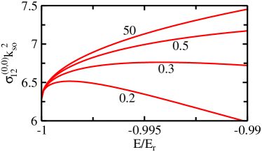
Figure 2: (Color online) Illustration of the threshold behavior for the $(J,M_{J})=(0,0)$ channel. The solid lines show the partial cross sections $\sigma_{12}^{(0,0)}=\sigma_{22}^{(0,0)}$, in units of $1/k_{\text{so}}^{2}$, as a function of the energy $E$ in the vicinity of $E=-E_{r}$ for four different $|a_{s}k_{\text{so}}|$, $|a_{s}k_{\text{so}}|=0.2,0.3,0.5$ and $50$ (see labels in the figure). The partial cross section $\sigma_{12}^{(0,0)}$ is equal to $2\pi/k_{\text{so}}^{2}$ at $E=-E_{r}$ for all $|a_{s}k_{\text{so}}|$.

Since the first-order correction is also independent of $a_{s}$ (see Table 2), the variation of $\sigma_{jl}^{(0,0)}$ near $E=-E_{r}$ is the same for all $a_{s}$.

	$E\to-E_{r}$ $(a_{s}\neq 0)$
$\sigma_{11}^{(0,0)}k_{\text{so}}^{2}=\sigma_{21}^{(0,0)}k_{\text{so}}^{2}$	$2\pi-4\pi x-2\pi\left[(a_{s}k_{\text{so}})^{-2}+1\right]x^{2}$
$\sigma_{12}^{(0,0)}k_{\text{so}}^{2}=\sigma_{22}^{(0,0)}k_{\text{so}}^{2}$	$2\pi+4\pi x-2\pi\left[(a_{s}k_{\text{so}})^{-2}+1\right]x^{2}$

Table 2: New threshold behavior for two particles in the $(J,M_{J})=(0,0)$ channel near $E=-E_{r}$. The partial cross sections are independent of $a_{s}$ and approach, in units of $1/k_{\text{so}}^{2}$, the constant $2\pi$ at $E=-E_{r}$. The first-order correction is also independent of $a_{s}$ for all $\sigma_{jl}^{(0,0)}$. Here, we introduced the abbreviation $x=\sqrt{E/E_{r}+1}$.

We refer to this behavior as universal as it is fully determined by the single-particle quantity $k_{\text{so}}$. The energy range over which the first-order correction provides a good description depends on $a_{s}$. For large $|a_{s}k_{\text{so}}|$, the second-order correction is small. For small $|a_{s}k_{\text{so}}|$, in contrast, the second-order correction is significant, leading to a “turn-around” of $\sigma_{jl}^{(0,0)}$ (see, e.g., the lowest curve in Fig. 2 for $|a_{s}k_{\text{so}}|=0.2$). Since the isotropic three-dimensional spin-orbit coupling scenario has not yet been realized experimentally in cold atom systems, we use values from one-dimensional experimental realizations spielman to get a feeling for the scattering length values covered in Fig. 2. Using $k_{\text{so}}=\sqrt{2}\pi/\lambda$ and $\lambda\approx 804nm$, the values of $a_{s}k_{\text{so}}=0.2$ and $50$ correspond to $a_{s}\approx 680a_{0}$ and $170,000a_{0}$, where $a_{0}$ denotes the Bohr radius; such scattering length values can be realized by utilizing Feshbach resonance techniques chin . We also note that proposals for adjusting the spin-orbit coupling strength have been put forward tune_soc ; tune_soc2 ; tune_soc3 .

The asymptotic large $r$ basis chosen in our work and in Ref. xiaoling differ. Reference xiaoling used a rotated basis, which is related to our asymptotic basis through the application of the matrix $U$ [i.e., the matrices $\mathcal{J}^{(0,0)}(r)U$ and $\mathcal{N}^{(0,0)}(r)U$ are used instead of $\mathcal{J}^{(0,0)}(r)$ and $\mathcal{N}^{(0,0)}(r)$ as in our work], where $U$ is chosen such that $U^{-1}\mathcal{K}^{(0,0)}U$ and $U^{-1}\mathcal{S}^{(0,0)}U$ are diagonal. The incoming states of Ref. xiaoling cannot be labeled by a fixed momentum and instead are linear combinations of states with different momenta. Reference zhenhua , which also discussed the relationship between the different asymptotic basis, referred to these states as “standing waves”. Diagonalizing $\mathcal{K}^{(0,0)}$, one finds that one of the eigenvalues of $\mathcal{K}^{(0,0)}$ is 0 (this corresponds to a vanishing “effective” $p$-wave phase shift $\delta_{\text{eff}}^{p}$, i.e., $\delta_{\text{eff}}^{p}=0$) and that the other eigenvalue is given by the “effective” $s$-wave phase shift $\delta_{\text{eff}}^{s}$,

$$\text{tan}\delta_{\text{eff}}^{s}=-a_{s}k_{\text{so}}\left[\left(\frac{E}{E_{r}}+1\right)^{1/2}+\left(\frac{E}{E_{r}}+1\right)^{-1/2}\right].$$ (46)

Expression (46) agrees with Eq. (44) from Ref. xiaoling . The fact that one of the eigenvalues is zero is a consequence of the fact that our interaction potential $\hat{V}_{\text{ps}}$ does not account for a finite free-space $p$-wave phase shift. While Ref. zhenhua interpreted the phase shifts $\delta_{\text{eff}}^{s}$ and $\delta_{\text{eff}}^{p}$ as the equivalent of the usual free-space $s$- and $p$-wave phase shifts, we prefer to think of these phase shifts as effective phase shifts that are obtained by switching to the standing wave picture. The “true” phase shifts, defined in analogy to the standard partial wave decomposition, are those obtained by writing the elements of the matrix given in Eq. (43) as $\tan\delta_{jl}$.

In the “high energy” regime ($E\gg-E_{r}$), the first term in Eq. (46) dominates and the tangent of the phase shift is approximately proportional to the density of states of a three-dimensional system. Near the scattering threshold ($E\to-E_{r}$), the second term in Eq. (46) dominates and the tangent of the phase shift is approximately proportional to the density of states of a one-dimensional system. This effective dimensionality reduction is responsible for the emergence of the new universal threshold law (see Table 2). Equivalently, for $E\to-E_{r}$, the eigenvalue given in Eq. (46) diverges and both the $\mathcal{S}^{(0,0)}$ matrix and the partial cross sections are independent of $a_{s}$. As the above discussion shows, the analysis of the effective phase shifts, obtained by switching to the “standing wave” basis, provides a simple intuitive understanding of the modified threshold law discussed in the context of Table 2. Moreover, the standing wave basis does allow for the construction of effective low-energy interactions that may be easier to deal with in multi-body theories than the original pseudo-potential xiaoling ; zhenhua .

To determine the bound state energies, we calculate the poles of the $\mathcal{S}^{(0,0)}$ matrix. The bound state energy $E_{\text{bound}}^{(0,0)}$ is determined by the roots of the equation

$$\tan\delta_{\text{eff}}^{s}=-\imath.$$ (47)

In agreement with Refs. bound_shenoy ; xiaoling ; pengzhang ; zhenhua , we find that there exists a bound state for all $a_{s}$. The bound state energy reads

$$E_{\text{bound}}^{(0,0)}=-\frac{\hbar^{2}k_{*}^{2}}{2\mu}-E_{r},$$ (48)

where

$$k_{*}=\frac{1+\text{sign}(a_{s})\sqrt{1+4a_{s}^{2}k_{\text{so}}^{2}}}{2a_{s}}.$$ (49)

For $k_{\text{so}}=0$, Eqs. (48) and (49) reduce to the binding energy $-\hbar^{2}/(2\mu a_{s}^{2})$ for pure $s$-wave contact interactions with positive $a_{s}$.

IV $(J,M_{J})=(1,M_{J})$ channels

This section considers two particles in the $(J,M_{J})=(1,M_{J})$ channels, where $M_{J}$ takes the values $-1$, $0$ and $1$. While the radial parts of the wave functions for different $M_{J}$ are identical, the angular parts differ. Specifically, given the scattering wave function in the $M_{J}$ channel, that in the $M_{J}^{\prime}$ channel is obtained by replacing $|J,M_{J};L,S\rangle$ by $|J,M_{J}^{\prime};L,S\rangle$. Angular momentum algebra yields that the components $(J,M_{J};L,S)=(1,M_{J};1,0)$, $(1,M_{J};1,1)$, $(1,M_{J};2,1)$ and $(1,M_{J};0,1)$ contribute. For the $(J,M_{J})=(1,M_{J})$ channels, there exist two scattering thresholds, namely, $E=-\eta^{2}E_{r}$ and $E=-E_{r}$. For $E>-\eta^{2}E_{r}$, branch A and branch B are open. At $E=-\eta^{2}E_{r}$, branch B becomes closed, implying that branch A is the only open branch in the energy regime $-E_{r}<E<-\eta^{2}E_{r}$ (see the dispersion curves in Fig. 1). Using the projection procedure outlined in Sec. II, we have

$$\mathcal{J}^{(1,M_{J})}(r)=\begin{bmatrix}&\frac{\imath}{\sqrt{2}}N_{A_{+}}\bar{k}_{A_{+}}j_{1}(\bar{k}_{A_{+}}r)&\frac{\imath}{\sqrt{2}}N_{A_{-}}\bar{k}_{A_{-}}j_{1}(\bar{k}_{A_{-}}r)&0&0\\ &\frac{1}{\sqrt{6}}N_{A_{+}}\bar{k}_{A_{+}}j_{0}(\bar{k}_{A_{+}}r)&\frac{1}{\sqrt{6}}N_{A_{-}}\bar{k}_{A_{-}}j_{0}(\bar{k}_{A_{-}}r)&\frac{1}{\sqrt{3}}N_{B_{+}}\bar{k}_{B_{+}}j_{0}(\bar{k}_{B_{+}}r)&\frac{1}{\sqrt{3}}N_{B_{-}}\bar{k}_{B_{-}}j_{0}(\bar{k}_{B_{-}}r)\\ &\frac{1}{\sqrt{3}}N_{A_{+}}\bar{k}_{A_{+}}j_{2}(\bar{k}_{A_{+}}r)&\frac{1}{\sqrt{3}}N_{A_{-}}\bar{k}_{A_{-}}j_{2}(\bar{k}_{A_{-}}r)&-\frac{1}{\sqrt{6}}N_{B_{+}}\bar{k}_{B_{+}}j_{2}(\bar{k}_{B_{+}}r)&-\frac{1}{\sqrt{6}}N_{B_{-}}\bar{k}_{B_{-}}j_{2}(\bar{k}_{B_{-}}r)\\ &0&0&\frac{-\imath}{\sqrt{2}}N_{B_{+}}\bar{k}_{B_{+}}j_{1}(\bar{k}_{B_{+}}r)&\frac{-\imath}{\sqrt{2}}N_{B_{-}}\bar{k}_{B_{-}}j_{1}(\bar{k}_{B_{-}}r)\end{bmatrix},$$ (50)

$$\mathcal{N}^{(1,M_{J})}(r)=\begin{bmatrix}&\frac{\imath}{\sqrt{2}}N_{A_{+}}\bar{k}_{A_{+}}n_{1}(\bar{k}_{A_{+}}r)&-\frac{\imath}{\sqrt{2}}N_{A_{-}}\bar{k}_{A_{-}}n_{1}(\bar{k}_{A_{-}}r)&0&0\\ &\frac{1}{\sqrt{6}}N_{A_{+}}\bar{k}_{A_{+}}n_{0}(\bar{k}_{A_{+}}r)&-\frac{1}{\sqrt{6}}N_{A_{-}}\bar{k}_{A_{-}}n_{0}(\bar{k}_{A_{-}}r)&\frac{1}{\sqrt{3}}N_{B_{+}}\bar{k}_{B_{+}}n_{0}(\bar{k}_{B_{+}}r)&-\frac{1}{\sqrt{3}}N_{B_{-}}\bar{k}_{B_{-}}n_{0}(\bar{k}_{B_{-}}r)\\ &\frac{1}{\sqrt{3}}N_{A_{+}}\bar{k}_{A_{+}}n_{2}(\bar{k}_{A_{+}}r)&-\frac{1}{\sqrt{3}}N_{A_{-}}\bar{k}_{A_{-}}n_{2}(\bar{k}_{A_{-}}r)&-\frac{1}{\sqrt{6}}N_{B_{+}}\bar{k}_{B_{+}}n_{2}(\bar{k}_{B_{+}}r)&\frac{1}{\sqrt{6}}N_{B_{-}}\bar{k}_{B_{-}}n_{2}(\bar{k}_{B_{-}}r)\\ &0&0&\frac{-\imath}{\sqrt{2}}N_{B_{+}}\bar{k}_{B_{+}}n_{1}(\bar{k}_{B_{+}}r)&\frac{\imath}{\sqrt{2}}N_{B_{-}}\bar{k}_{B_{-}}n_{1}(\bar{k}_{B_{-}}r)\end{bmatrix},$$ (51)

and

$$\Psi^{(1,M_{J})}(r)=\mathcal{J}^{(1,M_{J})}(r)-\mathcal{N}^{(1,M_{J})}(r)\mathcal{K}^{(1,M_{J})}.$$ (52)

Assuming $E>-\eta^{2}E_{r}$ and following the same steps as in Sec. III, the $4$ by $4$ $\mathcal{K}^{(1,M_{J})}$ matrix is determined by matching the zero-range boundary conditions. We find

$$\mathcal{K}^{(1,M_{J})}=-\frac{a_{s}}{3(\bar{k}_{A_{+}}-\bar{k}_{A_{-}})}\begin{bmatrix}\bar{k}_{A_{+}}^{2}&\bar{k}_{A_{+}}\bar{k}_{A_{-}}&\beta\bar{k}_{A_{+}}\bar{k}_{B_{+}}&\beta\bar{k}_{A_{+}}\bar{k}_{B_{-}}\\ \bar{k}_{A_{+}}\bar{k}_{A_{-}}&\bar{k}_{A_{-}}^{2}&\beta\bar{k}_{A_{-}}\bar{k}_{B_{+}}&\beta\bar{k}_{A_{-}}\bar{k}_{B_{-}}\\ \beta\bar{k}_{A_{+}}\bar{k}_{B_{+}}&\beta\bar{k}_{A_{-}}\bar{k}_{B_{+}}&\beta^{2}\bar{k}_{B_{+}}^{2}&\beta^{2}\bar{k}_{B_{+}}\bar{k}_{B_{-}}\\ \beta\bar{k}_{A_{+}}\bar{k}_{B_{-}}&\beta\bar{k}_{A_{-}}\bar{k}_{B_{-}}&\beta^{2}\bar{k}_{B_{+}}\bar{k}_{B_{-}}&\beta^{2}\bar{k}_{B_{-}}^{2}\end{bmatrix},$$ (53)

where $\beta$ is equal to $\sqrt{2}N_{B_{+}}/N_{A_{+}}$. The energy-dependent $\mathcal{S}^{(1,M_{J})}$ matrix and partial cross sections $\sigma_{jl}^{(1,M_{J})}$, in turn, are obtained using Eqs. (28) and (38). Note, throughout the remainder of this section we drop the superscript “$(1,M_{J})$” from the partial cross sections $\sigma_{jl}^{(1,M_{J})}$ for notational convenience.

To obtain the partial cross sections for the energy region $-E_{r}<E<-\eta^{2}E_{r}$, we pursue two different but equivalent approaches. Approach 1 constructs a $4$ by $4$ $\mathcal{K}^{(1,M_{J})}$ matrix, partitions off the $2$ by $2$ $\mathcal{K}^{(1,M_{J})}_{oo}$ matrix, and then constructs the $2$ by $2$ $\mathcal{S}^{(1,M_{J})}_{oo}$ matrix. Approach 2 analytically continues the $4$ by $4$ $\mathcal{S}^{(1,M_{J})}$ matrix for $E>-\eta^{2}E_{r}$ to the $E<-\eta^{2}E_{r}$ energy region and then partitions off the $2$ by $2$ $\mathcal{S}^{(1,M_{J})}_{oo}$ matrix. In both approaches, the partial cross sections are obtained from the $2$ by $2$ $\mathcal{S}^{(1,M_{J})}_{oo}$ matrix.

Approach 1 follows the logic of Ref. johnson , which discusses multi-channel scattering in the absence of spin-orbit coupling. Since branch $B$ is closed in the energy region $-E_{r}<E<-\eta^{2}E_{r}$, $\bar{k}_{B_{+}}$ and $\bar{k}_{B_{-}}$ are imaginary. This motivates us to write $\bar{k}_{B_{+}}=\imath k^{*}-\eta k_{\text{so}}$ and $\bar{k}_{B_{-}}=-\imath k^{*}-\eta k_{\text{so}}$ with $k^{*}$ real and $k^{*}$ greater than zero. To ensure that the last two columns of $\mathcal{N}^{(1,M_{J})}(r)$ decay exponentially, we replace the $n_{j}(\bar{k}_{B_{+}}r)$ ($j=0,1$, and $2$) in the third column of $\mathcal{N}^{(1,M_{J})}(r)$ by $-n_{j}(\bar{k}_{B_{+}}r)+\imath j_{j}(\bar{k}_{B_{+}}r)$ and the $n_{j}(\bar{k}_{B_{-}}r)$ ($j=0,1$, and $2$) in the fourth column of $\mathcal{N}^{(1,M_{J})}(r)$ by $-n_{j}(\bar{k}_{B-}r)-\imath j_{j}(\bar{k}_{B_{-}}r)$. To determine the corresponding $\mathcal{K}^{(1,M_{J})}$ matrix, we plug $\mathcal{J}^{(1,M_{J})}(r)$, Eq. (50), and the modified $\mathcal{N}^{(1,M_{J})}(r)$ into Eq. (52). Matching the resulting $\Psi^{(1,M_{J})}(r)$ to the $s$-, $p$- and $d$-wave boundary conditions at $r=0$, we obtain a modified $4$ by $4$ $\mathcal{K}^{(1,M_{J})}$ matrix applicable to the energy regime $-E_{r}<E<-\eta^{2}E_{r}$. Dividing this matrix into the open-open sub-block $\mathcal{K}^{(1,M_{J})}_{oo}$, the closed-closed sub-block $\mathcal{K}^{(1,M_{J})}_{cc}$, the open-closed sub-block $\mathcal{K}^{(1,M_{J})}_{oc}$, and the closed-open sub-block $\mathcal{K}^{(1,M_{J})}_{co}$, we have

$$\mathcal{K}^{(1,M_{J})}=\begin{bmatrix}&\mathcal{K}^{(1,M_{J})}_{oo}&\mathcal{K}^{(1,M_{J})}_{oc}\\ &\mathcal{K}^{(1,M_{J})}_{co}&\mathcal{K}^{(1,M_{J})}_{cc}\end{bmatrix},$$ (54)

where the open-open block $\mathcal{K}^{(1,M_{J})}_{oo}$ reads

$$\mathcal{K}^{(1,M_{J})}_{oo}=\frac{-a_{\text{eff}}}{\bar{k}_{A_{+}}-\bar{k}_{A_{-}}}\begin{bmatrix}\bar{k}_{A_{+}}^{2}&\bar{k}_{A_{+}}\bar{k}_{A_{-}}\\ \bar{k}_{A_{+}}\bar{k}_{A_{-}}&\bar{k}_{A_{-}}^{2}\end{bmatrix}$$ (55)

with

$$a_{\text{eff}}=\frac{a_{s}k^{*}}{3k^{*}+2a_{s}\left[(\eta k_{\text{so}})^{2}-(k^{*})^{2}\right]}.$$ (56)

Interestingly, Eq. (55) is identical to Eq. (43) with $a_{s}$ replaced by $a_{\text{eff}}$. The quantity $a_{\text{eff}}$ can thus be interpreted as an effective scattering length, which is modified by the states in the closed branch B, that describes the scattering between the states in branch A. The $\mathcal{S}^{(1,M_{J})}_{oo}$ matrix is obtained using Eq. (28) with $\mathcal{K}^{(J,M_{J})}$ replaced by $\mathcal{K}^{(J,M_{J})}_{oo}$. Last, the partial cross sections $\sigma_{11}$, $\sigma_{12}$, $\sigma_{21}$, and $\sigma_{22}$ for $-E_{r}\leq E<-\eta^{2}E_{r}$ are obtained using Eq. (38) with $\mathcal{S}^{(J,M_{J})}$ replaced by $\mathcal{S}^{(1,M_{J})}_{oo}$.

Approach 2 is based on analytic continuation. While this approach may be more intuitive to some readers, we note that the approach may be impractical for numerical calculations that propagate the logarithmic derivative matrix. Approach 2 takes the $4$ by $4$ $\mathcal{S}^{(1,M_{J})}$ matrix for $E>-\eta^{2}E_{r}$ and replaces $\bar{k}_{B_{+}}$ and $\bar{k}_{B_{-}}$ by (this is the same as in approach 1), respectively, $\imath k^{*}-\eta k_{\text{so}}$ and $-\imath k^{*}-\eta k_{\text{so}}$, where $k^{*}$ is real and greater than zero. These replacements guarantee that the outgoing solutions $\psi_{B}^{(1,M_{J})+}(\bar{k}_{B_{+}}r)$ and $\psi_{B}^{(1,M_{J})-}(\bar{k}_{B_{-}}r)$ decay exponentially for $E<-\eta^{2}E_{r}$. We then divide $\mathcal{S}^{(1,M_{J})}$ into the open-open sub-block $\mathcal{S}^{(1,M_{J})}_{oo}$, the closed-closed sub-block $\mathcal{S}^{(1,M_{J})}_{cc}$, the open-closed sub-block $\mathcal{S}^{(1,M_{J})}_{oc}$, and the closed-open sub-block $\mathcal{S}^{(1,M_{J})}_{co}$,

$$\mathcal{S}^{(1,M_{J})}=\begin{bmatrix}&\mathcal{S}^{(1,M_{J})}_{oo}&\mathcal{S}^{(1,M_{J})}_{oc}\\ &\mathcal{S}^{(1,M_{J})}_{co}&\mathcal{S}^{(1,M_{J})}_{cc}\end{bmatrix}.$$ (57)

The $\mathcal{S}^{(1,M_{J})}_{oo}$ matrix obtained from approach 2 agrees, as it should, with that obtained from approach 1.

We first analyze the scattering between branch A states, i.e., we analyze the partial cross sections $\sigma_{jl}$ with $j,l$ equal to $1$ and $2$. The threshold behavior is obtained by Taylor expanding $\sigma_{11}=\sigma_{21}$ and $\sigma_{12}=\sigma_{22}$ around $E=-\eta^{2}E_{r}$ (this is the energy where branch B becomes closed) and $E=-E_{r}$ (this is the lowest scattering threshold). Table 3 shows the leading and sub-leading terms for $\eta\neq 0$ (columns 2-4) and $\eta=0$ (columns 5-7).

	$E\to(-\eta^{2}E_{r})^{+}$	$E\to(-\eta^{2}E_{r})^{-}$	$E\to-E_{r}$	$E\to 0^{+}$	$E\to 0^{-}$	$E\to-E_{r}$
	$(\eta,a_{s}\neq 0)$	$(\eta,a_{s}\neq 0)$	$(\eta,a_{s}\neq 0)$	$(\eta=0,a_{s}\neq 0)$	$(\eta=0,a_{s}\neq 0)$	($\eta=0$, $a_{s}\neq 0$)
$\sigma_{11}k_{\text{so}}^{2}=\sigma_{21}k_{\text{so}}^{2}$	$c_{11}^{(0)}y^{2}+c_{11}^{(1+)}y^{3}$	$c_{11}^{(0)}y^{2}+{c_{11}^{(1-)}y^{3}}/{(a_{s}k_{\text{so}})}$	$2\pi-4\pi x$	$d_{11}^{(0)}y^{4}+d_{11}^{(1)}y^{5}$	$d_{11}^{(0)}y^{4}+{3d_{11}^{(1)}y^{5}}/{(2a_{s}k_{\text{so}})}$	$2\pi-4\pi x$
$\sigma_{12}k_{\text{so}}^{2}=\sigma_{22}k_{\text{so}}^{2}$	$c_{12}^{(0)}y^{2}+c_{12}^{(1+)}y^{3}$	$c_{12}^{(0)}y^{2}+{c_{12}^{(1-)}y^{3}}/{(a_{s}k_{\text{so}})}$	$2\pi+4\pi x$	$d_{12}^{(0)}+d_{12}^{(1)}y$	$d_{12}^{(0)}+{3d_{12}^{(1)}y}/{(2a_{s}k_{\text{so}})}$	$2\pi+4\pi x$

Table 3: Behavior of the partial cross sections for two particles with unequal masses ($\eta\neq 0$) and equal masses ($\eta=0$) in the $(J,M_{J})=(1,M_{J})$ channels; this table considers scattering processes within branch A. The superscript “$+$” indicates that the limit is taken from above (positive side) while the superscript “$-$” indicates that it is taken from below (negative side). The coefficients $c_{11}^{(0)}$, $c_{11}^{(1+)}$, $c_{11}^{(1-)}$, $c_{12}^{(0)}$, $c_{12}^{(1+)}$, and $c_{12}^{(1-)}$ for $\eta\neq 0$, which are reported in Appendix A, are independent of $a_{s}$. In contrast, the coefficients $d_{11}^{(0)}$, $d_{11}^{(1)}$, $d_{12}^{(0)}$, and $d_{12}^{(1)}$ for $\eta=0$, which are also reported in Appendix A, depend on $a_{s}^{2}$. The quantity $x$ is defined in the caption of Table 2 and $y$ is equal to $\sqrt{|E/E_{r}+\eta^{2}|}$.

It can be seen that the sub-leading term of $\sigma_{jl}$ behaves differently for $E\to(-\eta^{2}E_{r})^{+}$ and $E\to(-\eta^{2}E_{r})^{-}$. This “asymmetric” behavior is exemplarily shown in Fig. 3 for $\sigma_{12}k_{\text{so}}^{2}$ for $a_{s}k_{\text{so}}=1$ (circles) and $a_{s}k_{\text{so}}=-1$ (solid lines).

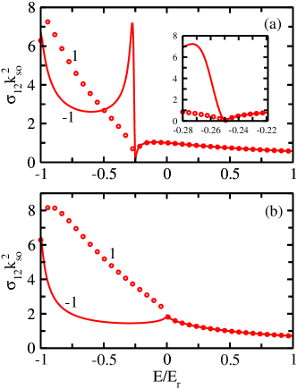
Figure 3: (Color online) Partial cross section $\sigma_{12}=\sigma_{22}$, in units of $1/k_{\text{so}}^{2}$, for the $(J,M_{J})=(1,M_{J})$ channels as a function of the energy $E$ for (a) unequal masses ($\eta=1/2$) and (b) equal masses ($\eta=0$); this figure considers scattering processes within branch A. The red solid curves correspond to $a_{s}k_{\text{so}}=-1$ and the circles to $a_{s}k_{\text{so}}=1$. For $E\geq-\eta^{2}E_{r}$, the partial cross section is independent of the sign of the $s$-wave scattering length, i.e., the solid curves and the circles coincide. For $-E_{r}\leq E<-\eta^{2}E_{r}$, in contrast, the partial cross section depends on the sign of $a_{s}$. The inset in panel (a) shows an enlargement of the $E\approx-\eta^{2}E_{r}$ region, demonstrating that the partial cross section changes continuously with energy.

The scattering threshold is equal to $-E_{r}/4$ for $\eta=1/2$ [see Fig. 3(a)] and equal to $0$ for $\eta=0$ [see Fig. 3(b)]. Figure 3 also illustrates another important aspect. The partial wave cross section $\sigma_{12}$ is independent of the sign of the scattering length $a_{s}$ for $E>-\eta^{2}E$ if $\eta$ is finite and for $E>0$ if $\eta$ is zero. The sign of the scattering length does, however, enter into the partial cross section expressions below these energies. The same holds true for $\sigma_{11}=\sigma_{21}$. This results from the fact that the partial cross sections $\sigma_{jl}$ ($j,l=1$ and 2) depend on $a_{s}^{2}$ for $E>-\eta^{2}E_{r}$ and on $a_{\text{eff}}^{2}$ for $E<-\eta^{2}E_{r}$. While $a_{s}^{2}$ is independent of the sign of $a_{s}$, $a_{\text{eff}}^{2}$ depends on the sign of $a_{s}$ [see Eq. (56)]. This behavior should be contrasted with the usual $s$-wave case, where the cross section is independent of the sign of the $s$-wave scattering length for all positive energies, implying that cross section measurements can only be used to deduce the magnitude of the scattering length but not the sign. Another aspect illustrated by Fig. 3 is that $\sigma_{12}$ vanishes at $E=-\eta^{2}E_{r}$ for $\eta=1/2$ and is finite for $\eta=0$. This can be understood by evaluating $a_{\text{eff}}$, Eq. (56), for $E=-\eta^{2}E_{r}$ ($k^{*}=0$). For $\eta\neq 0$ and $E=-\eta^{2}E_{r}$, $a_{\text{eff}}$ is equal to zero, implying that the partial cross sections for branch A vanish at this energy. For $\eta=0$ and $E=0$, $a_{\text{eff}}$ is equal to $a_{s}/3$, implying that the partial cross sections for branch A are finite. The partial wave cross sections $\sigma_{jl}$ with $j,l$ equal to 1 and 2 approach $2\pi/k_{\text{so}}^{2}$ at the lowest scattering threshold, i.e., at $E=-E_{r}$ (see Fig. 3 and columns 4 and 7 of Table 3). Importantly, the sub-leading term is—as in the $(J,M_{J})=(0,0)$ channel—independent of $a_{s}$ ($a_{s}\neq 0$) for vanishing and finite $\eta$. This can be interpreted, as in Sec. III, as a consequence of an effective dimensionality reduction.

Figure 4 highlights a number of other characteristics of the partial cross sections $\sigma_{12}$ and $\sigma_{11}$ in the vicinity of the threshold energies.

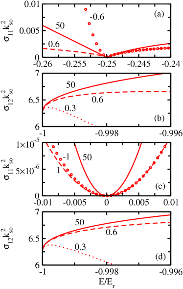
Figure 4: (Color online) Partial cross sections, in units of $1/k_{\text{so}}^{2}$, for the $(J,M_{J})=(1,M_{J})$ channels as a function of the energy $E$ for (a) and (b) unequal masses $(\eta=1/2)$, and (c) and (d) equal masses ($\eta=0$); this figure considers scattering processes within branch A. Panel (a) shows $\sigma_{11}k_{\text{so}}^{2}=\sigma_{21}k_{\text{so}}^{2}$ in the vicinity of $E=-\eta^{2}E_{r}$ for $a_{s}k_{\text{so}}=50$ (solid line), $a_{s}k_{\text{so}}=0.6$ (dashed line), and $a_{s}k_{\text{so}}=-0.6$ (circles). Panel (b) shows $\sigma_{12}k_{\text{so}}^{2}=\sigma_{22}k_{\text{so}}^{2}$ in the vicinity of $E=-E_{r}$ for $a_{s}k_{\text{so}}=50$ (solid line), $a_{s}k_{\text{so}}=0.6$ (dashed line), and $a_{s}k_{\text{so}}=0.3$ (dotted line). Panel (c) shows $\sigma_{11}k_{\text{so}}^{2}=\sigma_{21}k_{\text{so}}^{2}$ in the vicinity of $E=0$ for $a_{s}k_{\text{so}}=50$ (solid line), $a_{s}k_{\text{so}}=1$ (dashed line), and $a_{s}k_{\text{so}}=-1$ (circles). Panel (d) shows $\sigma_{12}k_{\text{so}}^{2}=\sigma_{22}k_{\text{so}}^{2}$ in the vicinity of $E=-E_{r}$ for $a_{s}k_{\text{so}}=50$ (solid line), $a_{s}k_{\text{so}}=0.6$ (dashed line), and $a_{s}k_{\text{so}}=0.3$ (dotted line).

For $\eta\neq 0$, the leading order term of $\sigma_{11}$ in the vicinity of $E=-\eta^{2}E_{r}$ goes to zero linearly with $|E+\eta^{2}E_{r}|$, with a coefficient that is independent of $a_{s}$. The sub-leading term of $\sigma_{11}$ scales as $|E+\eta^{2}E_{r}|^{3/2}$ and is independent of $a_{s}$ for $E\to(-\eta^{2}E_{r})^{+}$ but dependent on $a_{s}$ for $E\to(-\eta^{2}E_{r})^{-}$. This implies that $\sigma_{11}$ depends very weakly on $a_{s}$ for $E\to(-\eta^{2}E_{r})^{+}$ and comparatively strongly on $a_{s}$ for $E\to(-\eta^{2}E_{r})^{-}$. This discussion explains the asymmetry of the partial cross section $\sigma_{11}$ in the vicinity of $E=-\eta^{2}E_{r}$ in Fig. 4(a).

For $\eta=0$, in contrast, the leading order term of $\sigma_{11}$ in the vicinity of $E=0$ goes to zero quadratically with $E$, with a coefficient that depends on $a_{s}$ for $E<0$ and on $|a_{s}|$ for $E>0$ [see Fig. 4(c)]. Figures 4(b) and 4(d) show the threshold behavior of $\sigma_{12}$ for $\eta=1/2$ and $\eta=0$, respectively, in the vicinity of $E=-E_{r}$ for $a_{s}k_{\text{so}}=50$, $0.6$ and $0.3$ (see the labels in the figure). These figures illustrate the dependence of the partial cross section on $a_{s}k_{\text{so}}$.

Next, we analyze the partial cross sections $\sigma_{33}$, $\sigma_{34}$, $\sigma_{43}$ and $\sigma_{44}$, which describe the scattering between states in branch B. We Taylor expand $\sigma_{33}=\sigma_{34}$ and $\sigma_{43}=\sigma_{44}$ for $\eta>0$ around $E=-\eta^{2}E_{r}$ (see column 2 of Table 4). Since branch B is closed below $E=-\eta^{2}E_{r}$, the Taylor series is only applicable to the energy regime $E\geq-\eta^{2}E_{r}$. For $\eta\neq 0$, $\sigma_{33}=\sigma_{34}$ and $\sigma_{43}=\sigma_{44}$ approach the constant $2\pi/(\eta^{2}k_{\text{so}}^{2})$ (at this threshold all other partial cross sections go to zero, provided $\eta$ is greater than $0$; see Tables 3-6). Figures 5(a) and 5(b) show $\sigma_{33}$ and $\sigma_{34}$, respectively, in the vicinity of $E=-\eta^{2}E_{r}$ for $\eta=1/2$ and three different $|a_{s}k_{\text{so}}|$ combinations, i.e., for $|a_{s}k_{\text{so}}|=50$, $0.6$, and $0.3$.

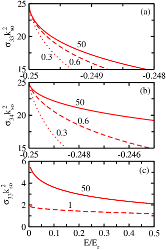
Figure 5: (Color online) Partial cross sections, in units of $1/k_{\text{so}}^{2}$, for the $(J,M_{J})=(1,M_{J})$ channels as a function of the energy $E$ for (a) and (b) unequal masses $(\eta=1/2)$, and (c) equal masses ($\eta=0$); this figure considers scattering processes within branch B. Panels (a) and (b) show $\sigma_{33}k_{\text{so}}^{2}=\sigma_{43}k_{\text{so}}^{2}$ and $\sigma_{34}k_{\text{so}}^{2}=\sigma_{44}k_{\text{so}}^{2}$, respectively, in the vicinity of $E=-\eta^{2}E_{r}$ for $|a_{s}k_{\text{so}}|=50$ (solid line), $|a_{s}k_{\text{so}}|=0.6$ (dashed line), and $|a_{s}k_{\text{so}}|=0.3$ (dotted line). Panel (c) shows $\sigma_{33}k_{\text{so}}^{2}=\sigma_{34}k_{\text{so}}^{2}=\sigma_{43}k_{\text{so}}^{2}=\sigma_{44}k_{\text{so}}^{2}$ in the vicinity of $E=0$ for $|a_{s}k_{\text{so}}|=50$ (solid line) and $|a_{s}k_{\text{so}}|=1$ (dashed line).

To obtain the threshold behavior for $\eta=0$, we set $\eta$ to $0$ and Taylor expand $\sigma_{33}=\sigma_{34}$ and $\sigma_{43}=\sigma_{44}$ around $E=0$. The resulting leading-order terms (see column 3 of Table 4) are equal to each other and depend on $a_{s}^{2}$.

	$E\to(-\eta^{2}E_{r})^{+}$	$E\to 0^{+}$
	$(\eta,a_{s}\neq 0)$	$(\eta=0,a_{s}\neq 0)$
$\sigma_{33}k_{\text{so}}^{2}=\sigma_{43}k_{\text{so}}^{2}$	${2\pi}/{\eta^{2}}$	${8\pi a_{s}^{2}k_{\text{so}}^{2}}/{(9+4a_{s}^{2}k_{\text{so}}^{2})}$
$\sigma_{34}k_{\text{so}}^{2}=\sigma_{44}k_{\text{so}}^{2}$	${2\pi}/{\eta^{2}}$	${8\pi a_{s}^{2}k_{\text{so}}^{2}}/{(9+4a_{s}^{2}k_{\text{so}}^{2})}$

Table 4: Behavior of the partial cross sections for two particles with unequal masses ($\eta\neq 0$) and equal masses ($\eta=0$) in the $(J,M_{J})=(1,M_{J})$ channels in the vicinity of the energy where branch B becomes closed; this table considers scattering processes within branch B. The leading term for $\eta\neq 0$ is constant (independent of $a_{s}$). In contrast, the leading term for $\eta=0$ depends on $a_{s}^{2}$.

In fact, all four partial cross sections $\sigma_{33}$, $\sigma_{43}$, $\sigma_{34}$, and $\sigma_{44}$ coincide for all positive energies. Figure 5(c) shows $\sigma_{33}=\sigma_{34}$ for $\eta=0$ with $|a_{s}k_{\text{so}}|=50$ and $1$.

Next, we analyze the partial cross sections $\sigma_{13}$, $\sigma_{14}$, $\sigma_{23}$ and $\sigma_{24}$, which describe scattering processes from states in branch A to states in branch B. Taylor expanding $\sigma_{13}=\sigma_{23}$ and $\sigma_{14}=\sigma_{24}$ around $E=-\eta^{2}E_{r}$, we find that the leading order term—assuming $E\geq-\eta^{2}E_{r}$—is proportional to $\sqrt{|E+\eta^{2}E_{r}|}$ for $\eta\neq 0$ and $\eta=0$ (see Table 5).

	$E\to(-\eta^{2}E_{r})^{+}$	$E\to 0^{+}$
	$(\eta,a_{s}\neq 0)$	$(\eta=0,a_{s}\neq 0)$
$\sigma_{13}k_{\text{so}}^{2}=\sigma_{23}k_{\text{so}}^{2}$	$c_{13}^{(0)}y$	$d_{13}^{(0)}y$
$\sigma_{14}k_{\text{so}}^{2}=\sigma_{24}k_{\text{so}}^{2}$	$c_{14}^{(0)}y$	$d_{14}^{(0)}y$

Table 5: Behavior of the partial cross sections for two particles with unequal masses ($\eta\neq 0$) and equal masses ($\eta=0$) in the $(J,M_{J})=(1,M_{J})$ channels in the vicinity of the energy where branch B becomes closed; this table considers scattering processes from branch A to branch B. The coefficients $c_{13}^{(0)}$ and $c_{14}^{(0)}$ for $\eta\neq 0$, which are reported in Appendix A, are independent of $a_{s}$. In contrast, the coefficients $d_{13}^{(0)}$ and $d_{14}^{(0)}$ for $\eta=0$, which are also reported in Appendix A, depend on $a_{s}^{2}$.

The prefactor is independent of $a_{s}$ for $\eta\neq 0$ and depends quadratically on $a_{s}$ for $\eta=0$. Figures 6(a) and 6(b) illustrate the threshold behavior of the partial cross sections $\sigma_{13}$ and $\sigma_{14}$, respectively, for $\eta=1/2$ and three different $|a_{s}k_{\text{so}}|$ combinations, i.e., for $|a_{s}k_{\text{so}}|=50$, $0.6$, and $0.3$.

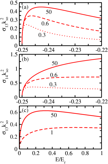
Figure 6: (Color online) Partial cross sections, in units of $1/k_{\text{so}}^{2}$, for the $(J,M_{J})=(1,M_{J})$ channels as a function of the energy $E$ for (a) and (b) unequal masses $(\eta=1/2)$, and (c) equal masses ($\eta=0$); this figure considers scattering processes from branch A to branch B. Panel (a) shows $\sigma_{13}k_{\text{so}}^{2}=\sigma_{23}k_{\text{so}}^{2}$ in the vicinity of $E=-\eta^{2}E_{r}$ for $a_{s}k_{\text{so}}=50$ (solid line), $a_{s}k_{\text{so}}=0.6$ (dashed line), and $a_{s}k_{\text{so}}=0.3$ (dotted line). Panel (b) shows $\sigma_{14}k_{\text{so}}^{2}=\sigma_{24}k_{\text{so}}^{2}$ in the vicinity of $E=-\eta^{2}E_{r}$ for $a_{s}k_{\text{so}}=50$ (solid line), $a_{s}k_{\text{so}}=0.6$ (dashed line), and $a_{s}k_{\text{so}}=0.3$ (dotted line). Panel (c) shows $\sigma_{13}k_{\text{so}}^{2}=\sigma_{23}k_{\text{so}}^{2}=\sigma_{14}k_{\text{so}}^{2}=\sigma_{24}k_{\text{so}}^{2}$ in the vicinity of $E=0$ for $|a_{s}k_{\text{so}}|=50$ (solid line) and $|a_{s}k_{\text{so}}|=1$ (dashed line).

Close to $-\eta^{2}E_{r}$, the leading term dominates and all three curves coincide approximately. Figure 6(c) shows $\sigma_{13}=\sigma_{14}$ for $\eta=0$ and $|a_{s}k_{\text{so}}|=50$ (solid line) and $|a_{s}k_{\text{so}}|=1$ (dashed line). The partial cross sections near the $E=0$ threshold approach 0 with a slope that depends on $a_{s}^{2}$.

Finally, we analyze the partial cross sections $\sigma_{31}$, $\sigma_{41}$, $\sigma_{32}$ and $\sigma_{42}$, which describe scattering processes from states in branch B to states in branch A. Taylor expanding $\sigma_{31}=\sigma_{41}$ and $\sigma_{32}=\sigma_{42}$ around $E=-\eta^{2}E_{r}$ ($E\geq-\eta^{2}E_{r}$), we find that the leading order terms of these partial cross sections are, for $\eta>0$, independent of $a_{s}$ and proportional to $\sqrt{|E+\eta^{2}E_{r}|}$ (see Table 6).

	$E\to(-\eta^{2}E_{r})^{+}$	$E\to 0^{+}$
	$(\eta,a_{s}\neq 0)$	$(\eta=0,a_{s}\neq 0)$
$\sigma_{31}k_{\text{so}}^{2}=\sigma_{41}k_{\text{so}}^{2}$	$c_{31}^{(0)}y$	$d_{31}^{(0)}y^{3}$
$\sigma_{32}k_{\text{so}}^{2}=\sigma_{42}k_{\text{so}}^{2}$	$c_{32}^{(0)}y$	$d_{32}^{(0)}y^{-1}$

Table 6: Behavior of the partial cross sections for two particles with unequal masses ($\eta\neq 0$) and equal masses ($\eta=0$) in the $(J,M_{J})=(1,M_{J})$ channels in the vicinity of the energy where branch B becomes closed; this table considers scattering processes from branch B to branch A. The coefficients $c_{31}^{(0)}$ and $c_{32}^{(0)}$ for $\eta\neq 0$, which are reported in Appendix A, are independent of $a_{s}$. In contrast, the coefficients $d_{31}^{(0)}$ and $d_{32}^{(0)}$ for $\eta=0$, which are also reported in Appendix A, depend on $a_{s}^{2}$.

Figures 7(a) and 7(b) illustrate the threshold behaviors for $\sigma_{31}$ and $\sigma_{32}$, respectively, in the vicinity of $E=-\eta^{2}E_{r}$ for $\eta=1/2$ and $|a_{s}k_{\text{so}}|=50$, $0.6$, and $0.3$.

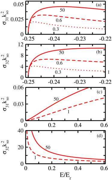
Figure 7: (Color online) Partial cross sections, in units of $1/k_{\text{so}}^{2}$, for the $(J,M_{J})=(1,M_{J})$ channels as a function of the energy $E$ for (a) and (b) unequal masses $(\eta=1/2)$, and (c) and (d) equal masses ($\eta=0$); this figure considers scattering processes from branch B to branch A. Panel (a) shows $\sigma_{31}k_{\text{so}}^{2}=\sigma_{41}k_{\text{so}}^{2}$ in the vicinity of $E=-\eta^{2}E_{r}$ for $|a_{s}k_{\text{so}}|=50$ (solid line), $|a_{s}k_{\text{so}}|=0.6$ (dashed line), and $|a_{s}k_{\text{so}}|=0.3$ (dotted line). Panel (b) shows $\sigma_{32}k_{\text{so}}^{2}=\sigma_{42}k_{\text{so}}^{2}$ in the vicinity of $E=-\eta^{2}E_{r}$ for $|a_{s}k_{\text{so}}|=50$ (solid line), $|a_{s}k_{\text{so}}|=0.6$ (dashed line), and $|a_{s}k_{\text{so}}|=0.3$ (dotted line). Panel (c) shows $\sigma_{31}k_{\text{so}}^{2}=\sigma_{41}k_{\text{so}}^{2}$ in the vicinity of $E=0$ for $|a_{s}k_{\text{so}}|=50$ (solid line) and $|a_{s}k_{\text{so}}|=1$ (dashed line). Panel (d) shows $\sigma_{32}k_{\text{so}}^{2}=\sigma_{42}k_{\text{so}}^{2}$ in the vicinity of $E=0$ for $|a_{s}k_{\text{so}}|=50$ (solid line) and $|a_{s}k_{\text{so}}|=1$ (dashed line).

Figures 7(c) and 7(d) show $\sigma_{31}$ and $\sigma_{32}$, respectively, for $\eta=0$ and $|a_{s}k_{\text{so}}|=50$ and $1$. For $\eta=0$, $\sigma_{31}=\sigma_{41}$ goes to zero at the $E=0$ threshold, with the leading order term depending on $a_{s}^{2}$, while $\sigma_{32}=\sigma_{42}$ diverges as $1/\sqrt{|E|}$, with the leading order term depending on $a_{s}^{2}$. We note that an analogous divergent behavior of a subset of the partial cross sections has been predicted for a spin-1 system with spin-orbit coupling chris .

As in Sec. III, we diagonalize the $\mathcal{K}^{(1,M_{J})}$ matrix for $E\geq-\eta^{2}E_{r}$ and the $\mathcal{K}^{(1,M_{J})}_{oo}$ matrix for $E<-\eta^{2}E_{r}$, and transform to the rotated or standing wave basis. For $E\geq-\eta^{2}E_{r}$, we find that three of the eigenvalues of $\mathcal{K}^{(1,M_{J})}$ are zero. If we had used a pseudo-potential that accounts not only for $s$-wave interactions but also for higher-partial wave interactions, these eigenvalues would not be zero. The fourth eigenvalue reads

$$\text{tan}\delta_{\text{eff,1}}^{s}=-\frac{a_{s}k_{\text{so}}}{3}\Bigg{[}\left(\frac{E}{E_{r}}+1\right)^{1/2}+\left(\frac{E}{E_{r}}+1\right)^{-1/2}+$$

$$2\left(\frac{E}{E_{r}}+\eta^{2}\right)^{1/2}+2\eta^{2}\left(\frac{E}{E_{r}}+\eta^{2}\right)^{-1/2}\Bigg{]}.$$ (58)

Equation (IV) shows that the threshold behavior around $-\eta^{2}E_{r}$ depends strongly on $\eta$. For $\eta=0$, the last term in square bracket in Eq. (IV) vanishes and $\tan\delta_{\text{eff},1}^{s}$ behaves like $-2a_{s}k_{\text{so}}(1+\sqrt{E/E_{r}})/3$ in the vicinity of $E=0$. This implies that the partial cross sections depend on $a_{s}$. For $\eta\neq 0$, the last term in square bracket in Eq. (IV), which behaves like a one-dimensional system, dominates (in fact, it diverges). Correspondingly, the partial cross sections are independent of $a_{s}$ as $E\rightarrow(-\eta^{2}E_{r})^{+}$.

For $E<-\eta^{2}E_{r}$, we find that one of the eigenvalues of $\mathcal{K}^{(1,M_{J})}_{oo}$ is zero while the other reads

$$\text{tan}\delta_{\text{eff,2}}^{s}=-a_{\text{eff}}k_{\text{so}}\left[\left(\frac{E}{E_{r}}+1\right)^{1/2}+\left(\frac{E}{E_{r}}+1\right)^{-1/2}\right].$$ (59)

Equation (59) shows that near the lowest scattering threshold $(E=-E_{r})$, the tangent of the phase shift is approximately proportional to the density of states of a one-dimensional system for both $\eta\neq 0$ and $\eta=0$ (i.e., the second term in the square bracket dominates as $E\to-E_{r}$). This is similar to what we found in Sec. III for the $(J,M_{J})=(0,0)$ channel. For $E=-E_{r}$, the tangent of the phase shift diverges and the partial cross sections are independent of $a_{s}$.

This section discussed the scattering processes within branch A (see Figs. 3 and 4 and Table 3), within branch B (see Fig. 5 and Table 4), from branch A to branch B (see Fig. 6 and Table 5), and from branch B to branch A (see Fig. 7 and Table 6) for the $(J,M_{J})=(1,M_{J})$ channels. As a means of summarizing, we consider the limiting values of the cross section matrices at the scattering thresholds. At the lowest scattering threshold ($E=-E_{r}$), the cross section matrix approaches, regardless of the mass ratio,

$$\sigma\xrightarrow{E=-E_{r}}\left[\begin{array}[]{cc}\frac{2\pi}{k_{\text{so}}^{2}}&\frac{2\pi}{k_{\text{so}}^{2}}\\ \frac{2\pi}{k_{\text{so}}^{2}}&\frac{2\pi}{k_{\text{so}}^{2}}\\ \end{array}\right].$$ (62)

For equal masses, the behavior of $\sigma_{12}$ is shown in Figs. 3(b) and 4(d). For unequal masses, the behavior of $\sigma_{12}$ is shown in Figs. 3(a) and 4(b). As already discussed, the mass ratio provides a means to tune the scattering threshold at which branch B becomes closed and, subsequently, to tune the threshold behavior. For equal masses, branch B becomes closed at $E=0$ and we have

$$\sigma\xrightarrow{E=0^{+}}\begin{bmatrix}0^{\ref{fig3b}\text{(c)}}&\frac{d_{12}^{(0)}(a_{s})}{k_{\text{so}}^{2}}^{\ref{fig3a}\text{(b)}}&0^{\ref{fig5}\text{(c)}}&0^{\ref{fig5}\text{(c)}}\\ 0^{\ref{fig3b}\text{(c)}}&\frac{d_{12}^{(0)}(a_{s})}{k_{\text{so}}^{2}}^{\ref{fig3a}\text{(b)}}&0^{\ref{fig5}\text{(c)}}&0^{\ref{fig5}\text{(c)}}\\ 0^{\ref{fig6}\text{(c)}}&\infty^{\ref{fig6}\text{(d)}}&\frac{d_{12}^{(0)}(a_{s})}{k_{\text{so}}^{2}}^{\ref{fig4}\text{(c)}}&\frac{d_{12}^{(0)}(a_{s})}{k_{\text{so}}^{2}}^{\ref{fig4}\text{(c)}}\\ 0^{\ref{fig6}\text{(c)}}&\infty^{\ref{fig6}\text{(d)}}&\frac{d_{12}^{(0)}(a_{s})}{k_{\text{so}}^{2}}^{\ref{fig4}\text{(c)}}&\frac{d_{12}^{(0)}(a_{s})}{k_{\text{so}}^{2}}^{\ref{fig4}\text{(c)}}\\ \end{bmatrix}.$$ (63)

For unequal masses, branch B becomes closed at $E=-\eta^{2}E_{r}$ and we instead have

$$\sigma\xrightarrow{E=-\eta^{2}E_{r}}\begin{bmatrix}0^{\ref{fig3b}\text{(a)}}&0^{\ref{fig3a}\text{(a)}}&0^{\ref{fig5}\text{(a)}}&0^{\ref{fig5}\text{(b)}}\\ 0^{\ref{fig3b}\text{(a)}}&0^{\ref{fig3a}\text{(a)}}&0^{\ref{fig5}\text{(a)}}&0^{\ref{fig5}\text{(b)}}\\ 0^{\ref{fig6}\text{(a)}}&0^{\ref{fig6}\text{(b)}}&\frac{2\pi}{\eta^{2}k_{\text{so}}^{2}}^{\ref{fig4}\text{(a)}}&\frac{2\pi}{\eta^{2}k_{\text{so}}^{2}}^{\ref{fig4}\text{(b)}}\\ 0^{\ref{fig6}\text{(a)}}&0^{\ref{fig6}\text{(b)}}&\frac{2\pi}{\eta^{2}k_{\text{so}}^{2}}^{\ref{fig4}\text{(a)}}&\frac{2\pi}{\eta^{2}k_{\text{so}}^{2}}^{\ref{fig4}\text{(b)}}\\ \end{bmatrix}.$$ (64)

In Eqs. (63) and (64), the superscript indicates the figure number in which the corresponding cross section is shown [e.g., the entry “$0^{\ref{fig3b}\text{(a)}}$” in Eq. (64) says that $\sigma_{11}$ is equal to zero at $E=-\eta^{2}E_{r}$ and that this behavior can be seen in Fig. 4(a)]. Comparison of Eqs. (63) and (64) shows that the threshold behavior is significantly impacted by the mass ratio.

To determine the bound state energies $E_{\text{bound}}^{(1,M_{J})}$ for the $(J,M_{J})=(1,M_{J})$ channels, we analyze the poles of the $\mathcal{S}^{(1,M_{J})}$ matrix. The bound state energy $E_{\text{bound}}^{(1,M_{J})}$ is determined by the roots of the equation

$$\tan\delta_{\text{eff,1}}^{s}=-\imath.$$ (65)

Since $\mathcal{S}^{(1,M_{J})}_{oo}$ is a sub-matrix of $\mathcal{S}^{(1,M_{J})}$, the poles of $\mathcal{S}^{(1,M_{J})}_{oo}$ are also poles of $\mathcal{S}^{(1,M_{J})}$. The equation $\tan\delta_{\text{eff,2}}^{s}=-\imath$ yields the same result for the bound state energy. In the weak-binding limit, i.e., for $1/a_{s}\to-\infty$, the bound state energy approaches $-(1+a_{s}^{2}k_{\text{so}}^{2}/9)E_{r}$. In the strong-binding limit, i.e., for $1/a_{s}\to+\infty$, the bound state energy approaches $-\hbar^{2}/(2\mu a_{s}^{2})-(1+2\eta^{2})E_{r}$. The solid, dashed and dotted lines in Fig. 8 show $E_{\text{bound}}^{(1,M_{J})}/E_{r}$, $E_{\text{bound}}^{(1,M_{J})}<-E_{r}$, as a function of $1/(a_{s}k_{\text{so}})$ for $\eta=0$, $1/2$ and $1$, respectively.

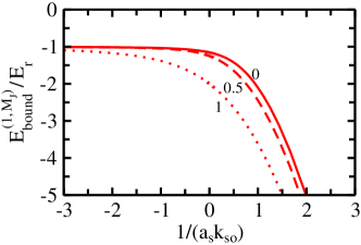
Figure 8: (Color online) Bound state energy $E_{\text{bound}}^{(1,M_{J})}$ for two particles in the $(J,M_{J})=(1,M_{J})$ channel. Solid, dashed and dotted lines show $E_{\text{bound}}^{(1,M_{J})}$ for $\eta=0$, $1/2$ and $1$, respectively. For increasing $\eta$, $E_{\text{bound}}^{(1,M_{J})}$ decreases, i.e., the dimer becomes—if the binding energy is measured in units of $E_{r}$—more strongly bound with increasing mass imbalance. In the extreme $\eta=1$ case, $E_{\text{bound}}^{(1,M_{J})}$ is identical to $E_{\text{bound}}^{(0,0)}$.

For all $\eta$, there exists a single two-body bound state for all $a_{s}$. For fixed $a_{s}k_{\text{so}}$, $E_{\text{bound}}^{(1,M_{J})}$ becomes more negative as $\eta$ increases from $0$ to $1$. For $\eta=1$, $E_{\text{bound}}^{(1,M_{J})}$ is identical to $E_{\text{bound}}^{(0,0)}$ since $\tan\delta_{\text{eff},1}^{s}$, Eq. (IV), agrees with $\tan\delta_{\text{eff}}^{s}$, Eq. (46), in this case.

V conclusion

This paper developed—building on the formulations presented in Refs. Gao ; chris for positive energies—a scattering framework for two particles with isotropic spin-orbit coupling applicable to all energies. Inspired by the usual partial wave decomposition for systems without spin-orbit coupling, Refs. Gao ; chris derived solutions using the magnitude of the wave number $k$. Since the derivative of the single particle energies with respect to $k$ for systems with isotropic spin-orbit coupling shows a discontinuity at vanishing energy [see Fig. 1(a)], the extension of the framework developed in Refs. Gao ; chris to negative energies is not entirely straightforward. One approach would be to obtain solutions for the various energy regions separately and to then match the solutions. Alternatively, and this is the route pursued in this paper, one might seek solutions that apply to all energy regions. To this end, we replaced $k$ by $\bar{k}$, $\bar{k}=h_{\text{rel}}k$, and defined single-particle energies whose derivative with respect to $\bar{k}$ is continuous for all energies [see Figs. 1(b) and 1(c)]. Our formulation allows us to treat the various scattering thresholds and energy variations across these thresholds using standard coupled-channel formulations. Specifically, this opens the door for calculating energy-dependent or thermally averaged scattering cross sections by making modifications to existing propagation based scattering codes.

We applied our framework to the $(J,M_{J})=(0,0)$ and $(J,M_{J})=(1,M_{J})$ channels for two particles, with equal or unequal masses, interacting through the zero-range $s$-wave pseudo-potential. Assuming $s$-wave contact interactions, the $J=0$ and $1$ channels are the only channels affected by the two-body interactions, i.e., the behavior of the $J=2,3,...$ channels is independent of $a_{s}$. If we, e.g., take the state $|\bar{k},\theta_{\mathbf{k}},\phi_{\mathbf{k}}\rangle_{A}$ as our initial state, the population of the $J=1$ partial wave channels is three times higher than that of the $J=0$ partial wave channel. If we take an equal mixture of $|\bar{k},\theta_{\mathbf{k}},\phi_{\mathbf{k}}\rangle_{A}$ and $|\bar{k},\theta_{\mathbf{k}},\phi_{\mathbf{k}}\rangle_{B}$ as our initial state, then the population of the $J=1$ partial wave channels is six times higher than that of the $J=0$ partial wave channel. While this paper did not report total cross sections, the above statements give a feeling for how to convert the partial wave cross sections presented in this paper to total cross sections.

We obtained closed analytical expressions applicable to all energies for the partial wave cross sections. The behavior of the partial cross sections was analyzed in detail near the scattering thresholds. Particular attention was paid to the scattering thresholds located at negative energies and simple analytical results were reported for the limiting behaviors. While our results were obtained for a specific functional form of the spin-orbit coupling and specific scattering channels, we believe that our study points toward more general characteristics of two-body scattering in the presence of spin-orbit coupling. First, the partial cross sections for scattering between states corresponding to a branch that becomes closed at a particular negative energy scattering threshold are—at the scattering threshold—independent of the $s$-wave scattering length $a_{s}$ and fully determined by the spin-orbit coupling strength $k_{\text{so}}$. This universal behavior can be interpreted as being a consequence of an effective dimensionality reduction near the scattering thresholds. At the lowest scattering threshold, all partial wave cross sections, and hence also the total cross section, are independent of $a_{s}$. Second, the mass ratio dependence of the results in the $(J,M_{J})=(1,M_{J})$ channels points toward an interesting tunability of few- and many-body properties of mass imbalanced systems. It is easily recognized that the scattering threshold where branch B becomes closed depends on the mass ratio. Since a subset of the partial cross sections vanishes at this threshold, different mass ratios should result in different energy dependent cross sections. Moreover, the two-body binding energy was found to depend on the mass ratio.

The present paper suggests a variety of follow-up studies. Most immediately, it would be interesting to extend our theoretical framework to systems with finite total momentum or with other types of spin-orbit coupling. Moreover, it would be interesting to incorporate the formulation presented in this paper into a two-body scattering code and to investigate the influence of two-body van der Waals physics on scattering observables in the presence of spin-orbit coupling. Looking further ahead, extending the scattering framework to three particles with spin-orbit coupling would be a major step forward.

VI acknowledgement

Support by the National Science Foundation through grant number PHY-1509892, discussions with X. Cui and Y. Yan, and comments on the manuscript by J. Jacob are gratefully acknowledged.

Appendix A Coefficients that describe the threshold behavior of the $(J,M_{J})=(1,M_{J})$ channel

In the following we report explicit expressions for the coefficients introduced in Table 3:

$$c_{11}^{(0)} = \frac{\pi}{2(1-\eta^{2})(1+\sqrt{1-\eta^{2}})^{2}},$$ (66)

$$c_{11}^{(1+)} = \frac{\eta^{2}-2}{\eta^{2}(1-\eta^{2})^{1/2}}c_{11}^{(0)},$$ (67)

$$c_{11}^{(1-)} = \frac{3}{\eta^{2}}c_{11}^{(0)},$$ (68)

$$c_{12}^{(0)} = \frac{\pi}{2(1-\eta^{2})(1-\sqrt{1-\eta^{2}})^{2}},$$ (69)

$$c_{12}^{(1+)} = \frac{\eta^{2}-2}{\eta^{2}(1-\eta^{2})^{1/2}}c_{12}^{(0)},$$ (70)

$$c_{12}^{(1-)} = \frac{3}{\eta^{2}}c_{12}^{(0)},$$ (71)

$$d_{11}^{(0)} = \frac{\pi a_{s}^{2}k_{\text{so}}^{2}}{2(9+4a_{s}^{2}k_{\text{so}}^{2})},$$ (72)

$$d_{11}^{(1)} = -\frac{16}{\pi}(d_{11}^{(0)})^{2},$$ (73)

$$d_{12}^{(0)} = 16d_{11}^{(0)},$$ (74)

and

$$d_{12}^{(1)}=-\frac{1}{\pi}(d_{12}^{(0)})^{2}.$$ (75)

In the following we report explicit expressions for the coefficients introduced in Table 5:

$$c_{13}^{(0)}=c_{14}^{(0)} = \frac{\pi}{\eta^{2}\sqrt{1-\eta^{2}}}$$ (76)

and

$$d_{13}^{(0)}=d_{14}^{(0)} = \frac{4\pi a_{s}^{2}k_{\text{so}}^{2}}{9+4a_{s}^{2}k_{\text{so}}^{2}}.$$ (77)

In the following we report explicit expressions for the coefficients introduced in Table 6:

$$c_{31}^{(0)} = 2\sqrt{1-\eta^{2}}c_{11}^{(0)},$$ (78)

$$c_{32}^{(0)} = 2\sqrt{1-\eta^{2}}c_{12}^{(0)},$$ (79)

$$d_{31}^{(0)} = \frac{1}{4}d_{13}^{(0)},$$ (80)

and

$$d_{32}^{(0)} = 4d_{13}^{(0)}.$$ (81)

References

(1)
G. Dresselhaus,
Spin-Orbit Coupling Effects in Zinc Blende Structures,
Phys. Rev. 100, 580 (1955).
(2)
Yu. A. Bychkov and E. I. Rashba,
Properties of a 2D electron gas with a lifted spectrum degeneracy,
Sov. Phys.- JETP Lett. 39, 78 (1984).
(3)
J. Struck,
C. Ölschläger, M. Weinberg, P. Hauke, J. Simonet, A. Eckardt, M. Lewenstein, K. Sengstock, and P. Windpassinger,
Tunable Gauge Potential for Neutral and Spinless Particles in Driven Optical Lattices,
Phys. Rev. Lett. 108, 225304 (2012).
(4)
Y.-J. Lin, K. Jiménez-García, and I. B. Spielman,
Spin-orbit-coupled Bose-Einstein condensates,
Nature (London) 471, 83 (2011).
(5)
L. W. Cheuk, A. T. Sommer, Z. Hadzibabic, T. Yefsah, W. S. Bakr, and M. W. Zwierlein,
Spin-Injection Spectroscopy of a Spin-Orbit Coupled Fermi Gas,
Phys. Rev. Lett. 109, 095302 (2012).
(6)
P. Wang, Z.-Q. Yu, Z. Fu, J. Miao, L. Huang, S. Chai, H. Zhai, and J. Zhang,
Spin-Orbit Coupled Degenerate Fermi Gases,
Phys. Rev. Lett. 109, 095301 (2012).
(7)
J.-Y. Zhang, S.-C. Ji, Z. Chen, L. Zhang, Z.-D. Du, B. Yan, G.-S. Pan, B. Zhao, Y.-J. Deng, H. Zhai, S. Chen, and J.-W. Pan,
Collective Dipole Oscillations of a Spin-Orbit Coupled Bose-Einstein Condensate,
Phys. Rev. Lett. 109, 115301 (2012).
(8)
L. Huang, Z. Meng, P. Wang, P. Peng, S.-L. Zhang, L. Chen, D. Li, Q. Zhou, and J. Zhang,
Experimental realization of two-dimensional synthetic spin-orbit coupling in ultracold Fermi gases,
Nat. Phys. 12, 540 (2016).
(9)
J. Dalibard, F. Gerbier, G. Juzeliūnas, and P. Öhberg,
Colloquium: Artificial gauge potentials for neutral atoms,
Rev. Mod. Phys. 83, 1523 (2011).
(10)
B. M. Anderson, G. Juzeliūnas, V. M. Galitski, and I. B. Spielman,
Synthetic 3D Spin-Orbit Coupling,
Phys. Rev. Lett. 108, 235301 (2012).
(11)
B. M. Anderson, I. B. Spielman, and G. Juzeliūnas,
Magnetically Generated Spin-Orbit Coupling for Ultracold Atoms,
Phys. Rev. Lett. 111, 125301 (2013).
(12)
J. Cserti, A. Csordás, and U. Zülicke,
Electronic and spin properties of Rashba billards,
Phys. Rev. B 70, 233307 (2004).
(13)
D. S. Novikov,
Elastic scattering theory and transport in graphene,
Phys. Rev. B 76, 245435 (2007).
(14)
J. Hutchinson and J. Maciejko,
Rashba scattering in the low-energy limit,
Phys. Rev. B 93, 245309 (2016).
(15)
A. J. Olson, S.-J. Wang, R. J. Niffenegger, C.-H. Li, C. H. Greene, and Y. P. Chen,
Tunable Landau-Zener transitions in a spin-orbit-coupled Bose-Einstein condensate,
Phys. Rev. A 90, 013616 (2014).
(16)
C. Qu, C. Hamner, M. Gong, C. Zhang, and P. Engels,
Observation of Zitterbewegung in a spin-orbit-coupled Bose-Einstein condensate,
Phys. Rev. A 88, 021604(R) (2013).
(17)
Y. Li, C. Qu, Y. Zhang, and C. Zhang,
Dynamical spin-density waves in a spin-orbit-coupled Bose-Einstein condensate,
Phys. Rev. A 92, 013635 (2015).
(18)
M. Gong, S. Tewari, and C. Zhang,
BCS-BEC Crossover and Topological Phase Transition in 3D Spin-Orbit Coupled Degenerate Fermi Gases,
Phys. Rev. Lett. 107, 195303 (2011).
(19)
H. Hu, L. Jiang, X.-J Liu, and H. Pu,
Probing Anisotropic Superfluidity in Atomic Fermi Gases with Rashba Spin-Orbit Coupling,
Phys. Rev. Lett. 107, 195304 (2011).
(20)
Z.-Q. Yu and H. Zhai,
Spin-Orbit Coupled Fermi Gases across a Feshbach Resonance,
Phys. Rev. Lett. 107, 195305 (2011).
(21)
J. P. Vyasanakere and V. B. Shenoy,
Bound states of two spin-1/2 fermions in a synthetic non-Abelian gauge field,
Phys. Rev. B 83, 094515 (2011).
(22)
J. P. Vyasanakere, S. Zhang, and V. B. Shenoy,
BCS-BEC crossover induced by a synthetic non-Abelian gauge field,
Phys. Rev. B 84, 014512 (2011).
(23)
J. P. Vyasanakere and V. B. Shenoy,
Rashbons: properties and their significance,
New. J. Phys. 14, 043041 (2012).
(24)
L. Han and C. A. R. Sá de Melo,
Evolution from BCS to BEC superfluidity in the presence of spin-orbit coupling,
Phys. Rev. A 85, 011606(R) (2012).
(25)
Z. Fu, L. Huang, Z. Meng, P. Wang, L. Zhang, S. Zhang, H. Zhai, P. Zhang, and J. Zhang,
Production of Feshbach molecules induced by spin-orbit coupling in Fermi gases,
Nat. Phys. 10, 110 (2014).
(26)
R. A. Williams, L. J. LeBlanc, K. Jiménez-García, M. C. Beeler, A. R. Perry, W. D. Phillips, and I. B. Spielman,
Synthetic Partial Waves in Ultracold Atomic Collisions,
Science 335, 314 (2012).
(27)
C. Wang, C. Gao, C.-M. Jian, and H. Zhai,
Spin-Orbit Coupled Spinor Bose-Einstein Condensates,
Phys. Rev. Lett. 105, 160403 (2010).
(28)
T.-L. Ho and S. Zhang,
Bose-Einstein Condensates with Spin-Orbit Interaction,
Phys. Rev. Lett. 107, 150403 (2011).
(29)
Y. Zhang, L. Mao, and C. Zhang,
Mean-Field Dynamics of Spin-Orbit Coupled Bose-Einstein Condensates,
Phys. Rev. Lett. 108, 035302 (2012).
(30)
Y. Li, G. I. Martone, L. P. Pitaevskii, and S. Stringari,
Superstripes and the Excitation Spectrum of a Spin-Orbit-Coupled Bose-Einstein Condensate,
Phys. Rev. Lett. 110, 235302 (2013).
(31)
X. Cui and T.-L. Ho,
Spin-orbit-coupled one-dimensional Fermi gases with infinite repulsion,
Phys. Rev. A 89, 013629 (2014).
(32)
Q. Guan and D. Blume,
Spin structure of harmonically trapped one-dimensional atoms with spin-orbit coupling,
Phys. Rev. A 92, 023641 (2015).
(33)
Z.-Y. Shi, X. Cui, and H. Zhai,
Universal Trimers Induced by Spin-Orbit Coupling in Ultracold Fermi Gases,
Phys. Rev. Lett. 112, 013201 (2014).
(34)
X. Cui and W. Yi,
Universal Borromean Binding in Spin-Orbit-Coupled Ultracold Fermi Gases,
Phys. Rev. X 4, 031026 (2014).
(35)
Z.-Y. Shi, H. Zhai, and X. Cui,
Efimov physics and universal trimers in spin-orbit-coupled ultracold atomic mixtures,
Phys. Rev. A 91, 023618 (2015).
(36)
H. Duan, L. You, and B. Gao,
Ultracold collisions in the presence of synthetic spin-orbit coupling,
Phys. Rev. A 87, 052708 (2013).
(37)
S.-J. Wang and C. H. Greene,
General formalism for ultracold scattering with isotropic spin-orbit coupling,
Phys. Rev. A 91, 022706 (2015).
(38)
L. Zhang, Y. Deng, and P. Zhang,
Scattering and effective interactions of ultracold atoms with spin-orbit coupling,
Phys. Rev. A 87, 053626 (2013).
(39)
P. Zhang, L. Zhang, and Y. Deng,
Modified Bethe-Peierls boundary condition for ultracold atoms with spin-orbit coupling,
Phys. Rev. A 86, 053608 (2012).
(40)
X. Cui,
Mixed-partial-wave scattering with spin-orbit coupling and validity of pseudopotentials,
Phys. Rev. A 85, 022705 (2012).
(41)
Y. Wu and Z. Yu,
Short-range asymptotic behavior of the wave functions of interacting spin-1/2 fermionic atoms with spin-orbit coupling: A model study,
Phys. Rev. A 87, 032703 (2013).
(42)
H. Zhai,
Degenerate quantum gases with spin-orbit coupling: a review,
Rep. Prog. Phys. 78, 026001 (2015).
(43)
There are three separate commutators to consider for the
-, - and -components of .
Moreover, since is a by
matrix, the commutator can be
broken down
into 16 separate commutators (and similarly for
and ).
(44)
Since the expectation value is
taken
with respect to
an
eigenstate of ,
we have
.
(45)
R. N. Zare, Angular Momentum: Understanding Spatial Aspects in Chemistry and Physics, 1st ed. (Wiley-Interscience, 1991).
(46)
Our current normalization condition differs from the Wronskian based normalization condition
in Ref. chris ;
as a result, the unit of our normalization constants differs from that of Ref. chris .
(47)
We refer to the as “partial cross sections”
since various combinations contribute to the scattering from channel
to channel .
Reference Gao used instead the term “cross section” and Ref. chris the term “(total) cross section”.
(48)
C. Chin, R. Grimm, P. Julienne, and E. Tiesinga,
Feshbach resonances in ultracold gases,
Rev. Mod. Phys. 82, 1225 (2010).
(49)
Y. Zhang, G. Chen, and C. Zhang,
Tunable Spin-orbit Coupling and Quantum Phase Transition in a Trapped Bose-Einstein Condensate,
Sci. Rep. 3, 1937 (2013).
(50)
K. Jiménez-García, L. J. LeBlanc, R. A. Williams, M. C. Beeler, C. Qu, M. Gong, C. Zhang, and I. B. Spielman,
Tunable Spin-Orbit Coupling via Strong Driving in Ultracold-Atom Systems,
Phys. Rev. Lett. 114, 125301 (2015).
(51)
X. Luo, L. Wu, J. Chen, Q. Guan, K. Gao, Z.-F Xu, L. You, and R. Wang,
Tunable atomic spin-orbit coupling synthesized with a modulating gradient magnetic field,
Sci. Rep. 6, 18983 (2016).
(52)
B. R. Johnson,
Comment on a recent criticism of the formula used to calculate the matrix in the multichannel log-derivative method,
Phys. Rev. A 32, 1241 (1985).