The Exchange Graphs of Weakly Separated Collections
Abstract.
Weakly separated collections arise in the cluster algebra derived from the Plücker coordinates on the nonnegative Grassmannian. Oh, Postnikov, and Speyer studied weakly separated collections over a general Grassmann necklace and proved the connectivity of every exchange graph. Oh and Speyer later introduced a generalization of exchange graphs that we call -constant graphs. They characterized these graphs in the smallest two cases. We prove an isomorphism between exchange graphs and a certain class of -constant graphs. We use this to extend Oh and Speyer’s characterization of these graphs to the smallest four cases, and we present a conjecture on a bound on the maximal order of these graphs. In addition, we fully characterize certain classes of these graphs in the special cases of cycles and trees.
1. Introduction
The notion of weak separation was introduced by Leclerc and Zelevinsky [1] in 1998 in the context of determining combinatorial criterion for the quasicommutativity of two quantum flag minors. The definition of weak separation requires the following definition of a cyclic ordering:
Definition 1.1.
For an integer , the integers are said to be cyclically ordered if there exists such that
Leclerc and Zelevinsky defined weak separation as follows:
Definition 1.2.
Let and be nonnegative integers such that . Two -element subsets are called weakly separated if there do not exist , cyclically ordered, with and , where denotes set-theoretic difference.
Remark 1.3.
This is equivalent to the condition that and are separated by some chord in the circle, i.e. that are cyclically ordered.
Leclerc and Zelevinsky [1] used the notion of weak separation to define certain collections of -elements subsets of for a fixed and . Let denote the collection of all -element subsets of . For nonnegative integers , a subset of the collection is called weakly separated if every two -elements subsets in are weakly separated. The subset is called a maximal weakly separated collection if is not contained in any larger weakly separated collection of .
Leclerc and Zelevinsky conjectured that any two maximal weakly separated collections of have the same cardinality and are linked by a sequence of cardinality-preserving operations called mutations. A mutation is defined as follows:
Definition 1.4.
Consider a set and let be cyclically ordered elements of Suppose that a maximal weakly separated collection contains and . Then the collection is said to be linked to by a mutation.
In 2005, Scott [6] proved that any weakly separated collection satisfies . This motivated him to make the following refined conjecture regarding the cardinality of maximal weakly separated collections: If is a maximal weakly separated collection, then the following is true:
| (1) |
In 2011, Oh, Postnikov, and Speyer [9] proved a generalization of by linking weak separation to certain graphs called plabic graphs through applying a previous work of Postnikov [5].
In 2006, Postnikov [5] studied total positivity on the Grassmannian. He defined the nonnegative Grassmannian as the part of the real Grassmannian in which all Plücker coordinates are nonnegative. He described a stratification of into positroid strata and combinatorially constructed their parametrization using plabic graphs. Namely, he proved that positroid cells can be parameterized through a certain type of planar bicolored graphs (plabic graphs). These type of graphs play an important role in the study of various mathematical objects, for example, appearing also in Kodama and Williams’s [3] study on KP-solitons.
Postnikov, Oh, and Speyer [9] used plabic graphs to prove Leclerc and Zelevinsky’s conjecture that any two maximal weakly separated collections in are linked by a sequence of mutations, from which followed. The main ingredient of their proof was their bijection between weakly separated collections and reduced plabic graphs. In fact, using this bijection, they were able to prove a generalization of based on extending the notion of a weakly separated collection to a general positroid. Their results had interesting consequences for cluster algebras. In 2003, Scott [7] had proved that the coordinate ring of , in its Plücker embedding, is a cluster algebra where the Plücker coordinates are the cluster variables. Postnikov, Oh, and Speyer [9] proved that the aforementioned clusters are in bijection with the maximal weakly collections of .
Our global aim is to continue the study of the combinatorial properties of the cluster algebra structure on . We specifically study weakly separated collections over a general positroid. In Section 2, we review important existing definitions and known results. In Section 3, we introduce some of our new definitions, state our main results, and outline the rest the paper.
2. Existing Definitions and Known Results
We review the relevant existing definitions, notation, and known results involving weakly separated collections. In Section 2.1, we review the definitions from [9] related to maximal weakly separated collections over a general positroid. In Section 2.2, we review the technology of plabic graphs from [9] and [5]. In Section 2.3, we review exchange graphs from [9] and the subgraphs from [8] that we call -constant graphs.
2.1. Weakly Separated Collections over a General Positroid
We recall the definitions and results from [9] relating to Grassmann necklaces, positroids, decorated permutations, and maximal weakly separated collections.
We define a connected Grassmann necklace.
Definition 2.1.
A connected Grassmann necklace is a sequence of -element subsets of such that, for , the set contains and (where we take the indices modulo ).
Remark 2.2.
All Grassmann necklaces that we will work with will be connected, though we will omit the word connected. For the rest of the paper, we assume that and .
We use the following notion of a linear order on .
Definition 2.3.
Consider positive integers . For , we say that if is a subsequence of For , we say that if and only if or .
Let and be -element subsets of such that and where and . Then we define the partial order
We now define the positroid associated to each Grassmann necklace.
Definition 2.4.
Given a Grassmann necklace , we define the positroid to be
This allows us to extend the notion of a maximal weakly separated collection to a general Grassmann necklace.
Definition 2.5.
For a Grassmann necklace , a weakly separated collection is said be over if is a subset of . The collection is said to be maximal over if is not contained in any larger weakly separated collection over .
Oh, Postnikov, and Speyer [9] proved a generalization of (Scott’s conjecture). Namely, they expressed the cardinality of every maximal weakly separated collection over a Grassmann necklace as a function of the decorated permutation associated to . We review the definitions relating to decorated permutations in the case of connected Grassmann necklaces.
Definition 2.6.
A connected decorated permutation is a permutation over such that there do not exist two circular intervals and such that and .
There is a simple relation between connected Grassmann necklaces and connected decorated permutations.
Proposition 2.7 (Oh, Postnikov, Speyer).
Connected Grassmann necklaces are in bijection with connected decorated permutations over .
Proof.
To go from a Grassmann necklace to a decorated permutation , we set
To go from a decorated permutation to a Grassmann necklace , we set
∎
Oh, Postnikov, and Speyer [9] defined the function (where is the set of permutations of ) as follows:
Definition 2.8.
For , the set forms an alignment in if are cyclically ordered (and all distinct). Let be the number of alignments in .
Oh, Postnikov, and Speyer [9] used the notion of a decorated permutation and the function to formulate their result involving cardinality. We recall the special case that corresponds to connected Grassmann necklaces:
Theorem 2.9 (Oh, Postnikov, Speyer).
Let be a maximal weakly separated collection over a connected Grassmann necklace . Suppose that has associated decorated permutation . Then the following is true:
2.2. Plabic Graphs
We define a plabic graph.
Definition 2.10.
A plabic graph (planar bicolored graph) is a planar undirected graph drawn inside a disk with vertices colored in black or white colors. The vertices on the boundary of the disk are called the boundary vertices. Suppose that there are boundary vertices. Then the boundary vertices are labeled in clockwise order by .
We define the strands in a plabic graph.
Definition 2.11.
A strand in a plabic graph is a directed path that satisfies the rules of the road: At every black vertex, the strand turns right, and at every white vertex, the strand turns left.
We define the criteria for a plabic graph to be reduced.
Definition 2.12.
A plabic graph is called reduced if the following holds:
-
•
A strand cannot form a closed loop in the interior of .
-
•
Any strand that passes through itself must be a simple loop that starts and ends at some boundary vertex.
-
•
For any two strands that have two vertices and in common, one strand must be directed from to , and the other strand must be directed from to .
Let be a reduced plabic graph. Then any strand in connects two boundary vertices. We associate a strand permutation with defined so that if the strand that starts at a boundary vertex ends at a boundary vertex . We label the strand that ends at boundary vertex by .
There are three types of moves on a plabic graph:
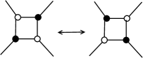
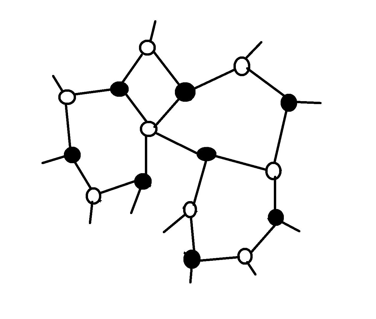
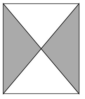
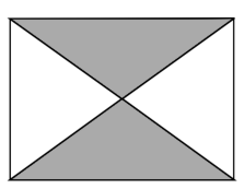
(M1)Pick a square with vertices alternating in colors as in Figure 1. Then we can switch the colors of these vertices.
(M2)Two adjoint vertices of the same color can be contracted into one vertex as in Figure 2.

(M3)We can insert or remove a vertex inside an edge as in Figure 3.

Postnikov [5] proved the following relation between strand permutations and the moves (M1), (M2), and (M3).
Theorem 2.13 (Postnikov).
Let and be two reduced plabic graphs with the same number of boundary vertices. Then if and only if can be obtained from by a sequence of moves (M1), (M2), and (M3).
We now describe the relation between reduced plabic graphs and weakly separated collections. We label the faces of a reduced plabic graph as follows: Let be a reduced plabic graph. For every , place inside every face that appears to the left of the strand labeled . Then the label of is the set of all integers placed inside . Let be the collection of sets of labels that occur on each face of the graph . Postnikov [5] showed that all the sets in have the same number of elements. We denote this number by . Oh, Postnikov, and Speyer [9] proved the following:
Theorem 2.14 (Oh, Postnikov, Speyer).
For a decorated permutation corresponding to a Grassmann necklace , a collection is a maximal weakly separated collection over if and only if it has the form for a reduced plabic graph with strand permutation .
We also consider a dual of plabic graphs called plabic tilings described in detail in [8]. The faces and vertices are flipped. In plabic tilings, the faces are colored black and white, and the vertices contain the sets of integer labels.
2.3. Exchange Graphs and -Constant Graphs
We review the definitions and known results regarding exchange graphs and -constant graphs.
For a given Grassmann necklace , the exchange graph is defined by the maximal weakly separated collections over under the mutation operation.
Definition 2.15.
Let be a Grassmann necklace and be the set of maximal weakly separated collections over . The exchange graph is defined as follows:
-
(1)
The vertices of are .
-
(2)
The vertices and are connected by an edge if and only if can be mutated into in one mutation.
In 2011, Oh, Postnikov, and Speyer [9] proved the following result:
Theorem 2.16 (Oh, Postnikov, Speyer).
Any exchange graph is connected.
Given an exchange graph and a weakly separated collection over , we call the -constant graph the subgraph defined by maximal weakly separated collections over that contain with edges defined by mutations of subsets not in .
Definition 2.17.
Let be a Grassmann necklace and be the set of maximal weakly separated collections over that contain . We call the -constant graph the vertex-induced subgraph of generated by . The co-dimension of is defined to be for
Remark 2.18.
Notice that -constant graphs are a generalization of exchange graphs. In fact, every exchange graph is isomorphic to a -constant graph: for any Grassmann necklace , we see that is isomorphic to
In 2014, Oh and Speyer [8] proved the following results:
Theorem 2.19 (Oh, Speyer).
Any -constant graph is connected.
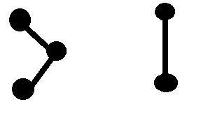
Theorem 2.20 (Oh, Speyer).
The only -constant graph with co-dimension is a path with vertex. The only -constant graphs with co-dimension are a path with vertex and a path with vertices.
3. Main Results
In Section 3.1, we present some of our new notions that are critical to understanding our main results. In Section 3.2, we present our main results along with an outline for the rest of the paper.
3.1. Some New Definitions
In Section 3.1.1, we present some basic definitions. In Section 3.1.2, we define special classes of exchange graphs and -constant graphs. In Section 3.1.3, we define equivalence classes of decorated permutations.
3.1.1. Basic Definitions
We define the following definitions and notation involving adjacency, interior size, and mutations.
We define two -elements subsets to be quasi-adjacent as follows:
Definition 3.1.
We call sets quasi-adjacent if .
Remark 3.2.
Suppose that and are contained in a maximal weakly separated collection . This definition is equivalent to the condition that and are on the same face in the plabic tiling of .
We now define a stronger notion of adjacency that is dependent on the choice of maximal weakly separated collection:
Definition 3.3.
Given a maximal weakly separated collection , we call two -element subsets adjacent if and only if in the plabic tiling of , there exists an edge between and that border a black face and a white face.
Remark 3.4.
Notice that all adjacent subsets are also quasi-adjacent.
We define the following notion with interior size which is closely related to cardinality:
Definition 3.5.
We define the of a maximal weakly separated collection over a Grassmann Necklace to be
Remark 3.6.
Notice that the interior size of is the number of sets in the interior of the plabic tiling of .
In fact, interior size is a property of the Grassmann necklace (and thus the exchange graph ). Let be the decorated permutation associated to . By Theorem 2.9, we know that the interior size of any maximal weakly separated collection in is . Thus, we let the interior size of both the Grassmann necklace and the exchange graph be this value. We denote this value by or .
We use the following notation and definitions to discuss mutations:
Definition 3.7.
Given a maximal weakly separated collection over a Grassmann Necklace , we say that a -element subset is in if in the plabic tiling of , the subset is surrounded by exactly 2 black faces and 2 white faces.
This means that we can mutate into a maximal weakly separated collection over that contains . Suppose that . We then say that can be mutated in into in . If is not surrounded by 2 black faces and 2 white faces, then we say that is in .
3.1.2. Special Classes of Exchange Graphs and -Constant Graphs
We define the applicable, mutation-friendly, and very-mutation-friendly conditions.
Roughly speaking, the applicable condition for a -constant graph requires that the sets in the weakly separated collection are connected to the boundary of the plabic tiling of for any maximal weakly separated collection .
Definition 3.8.
Consider a -constant graph . We say that is if for each set , there exists an integer and a weakly separated collection over satisfying the following properties:
-
(1)
is quasi-adjacent to for ,
-
(2)
-
(3)
and .
We use the following maximal weakly separated collection and Grassmann necklace as an example throughout the paper:
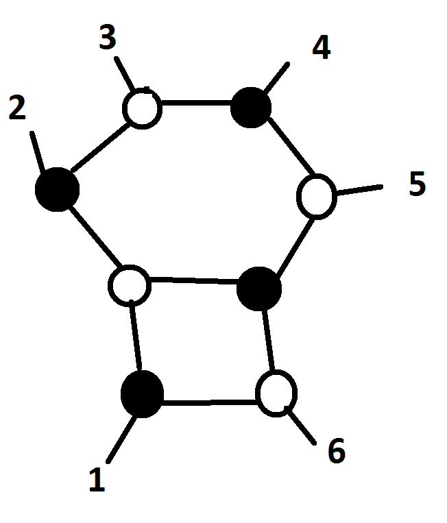
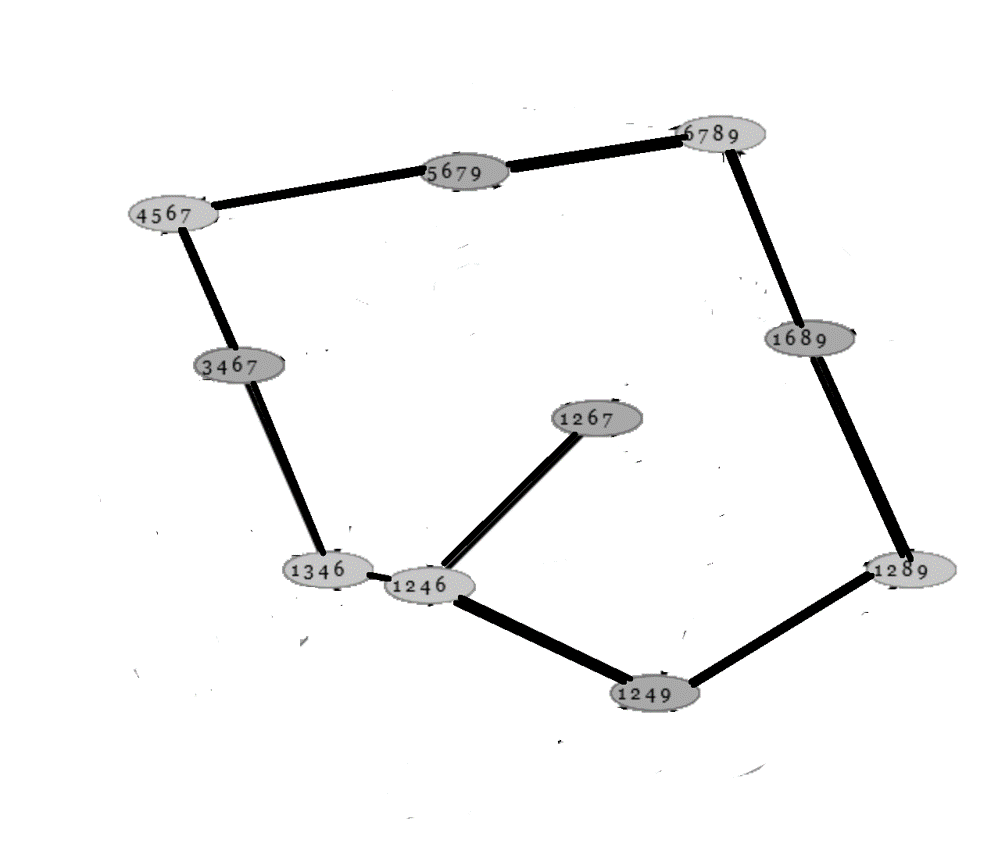
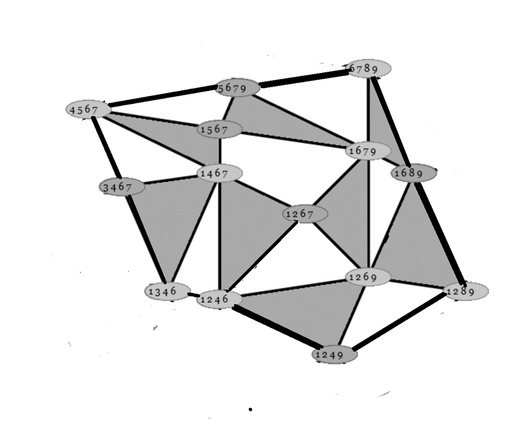
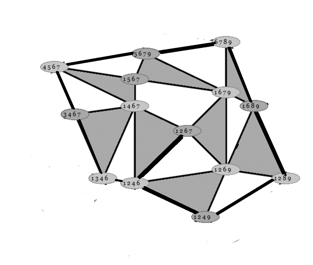
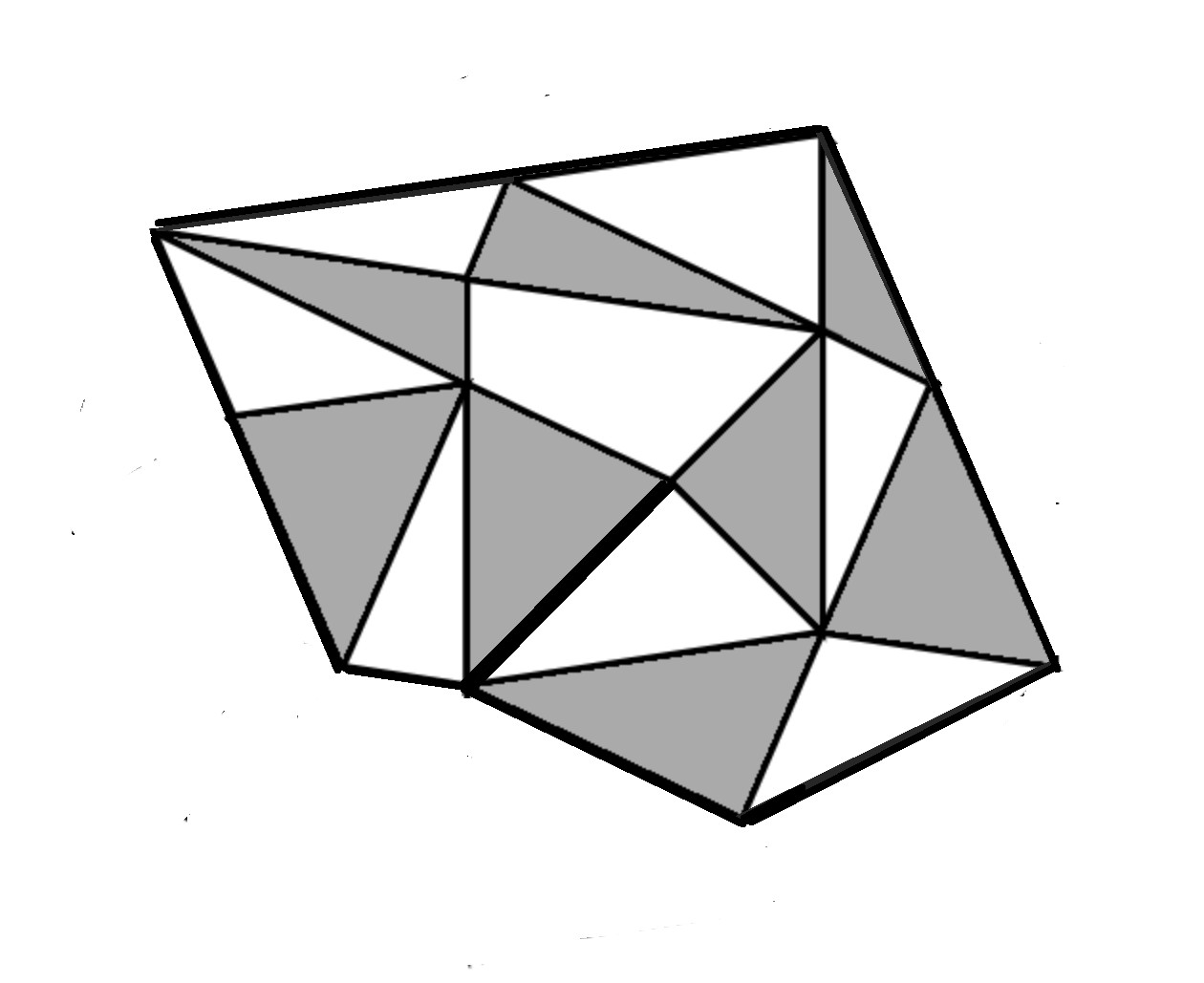
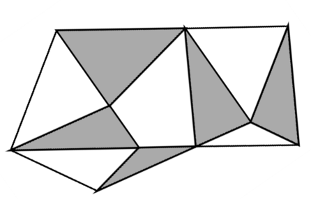
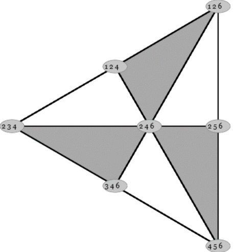
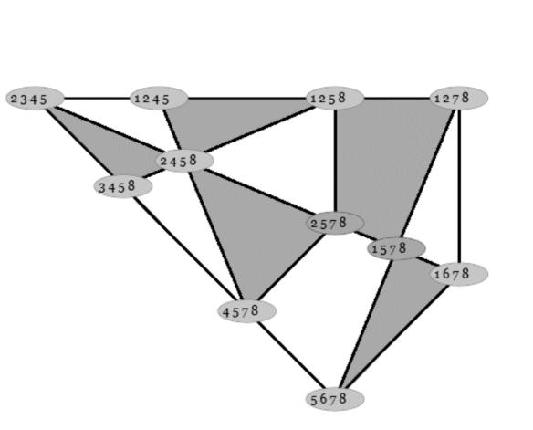
Example 3.9.
Consider the Grassmann necklace
Consider the maximal weakly separated collection that contains and the following subsets: , , , , , , , , , , , . Figure 4 shows the plabic tiling of .
Example 3.10.
Consider defined as in Example 3.9. Then we define the following weakly separated collections over :
The -constant graph is not applicable and the -constant graph is applicable.
Roughly speaking, the mutation-friendly condition for a Grassmann necklace requires that every subset in that is present in at least one maximal weakly separated collection in is mutatable in some maximal weakly separated collection in .
Definition 3.11.
A Grassmann necklace and its associated decorated permutation are if the intersection of all of the maximal weakly separated collections in is . We call an exchange graph mutation-friendly if and only if the Grassmann necklace is mutation-friendly.
Remark 3.12.
It follows from the definition that for a mutation-friendly exchange graph , we know that
We extend a similar notion to -constant graphs:
Definition 3.13.
A -constant graph is said to be if the intersection of all of the maximal weakly separated collections in is .
We define a stronger notion of the mutation-friendly condition in the case of exchange graphs. This condition, the very-mutation-friendly condition, requires that a certain sequence of -constant graphs of the exchange graph satisfy both the applicable and mutation-friendly conditions.
Definition 3.14.
A mutation-friendly Grassmann necklace with interior size is
if there exists a set of weakly separated collections satisfying the following properties:
-
(1)
is a weakly separated collection over containing for ,
-
(2)
for ,
-
(3)
for ,
-
(4)
and is applicable and mutation-friendly for
We call very-mutation-friendly if and only if is very-mutation-friendly.
3.1.3. Equivalence Classes
In order to simplify our discussion of Grassmann necklaces, we construct an equivalence class of decorated permutations that yield the same exchange graph. We show that exchange graphs are invariant under the following four operations on associated decorated permutations.
We first consider the inverse operation.
Proposition 3.15.
Let be the Grassmann necklace with decorated permutation and be the Grassmann necklace with decorated permutation Then the following is true:
Proof.
We must prove that there is a bijective mapping from the maximal weakly separated collections over to the maximal weakly separated collections over that preserves the mutation operation. Let take to where is obtained by flipping the colors of the vertices in the plabic graph of . ∎
Example 3.16.
We now consider label-reflection operations.
Definition 3.17.
For a positive integer , we define the label-reflection operation as follows. For an integer and a permutation of , we let be the permutation on defined so that for (where all numbers are considered modulo ).
Proposition 3.18.
Given integers , let be the Grassmann necklace with decorated permutation and be the Grassmann necklace with decorated permutation Then the following is true:
The proof is analogous to the proof of Proposition 3.15, except that is defined by reflecting the plabic graph of about the vertex labeled .
Example 3.19.
We now consider between-label-reflection operations.
Definition 3.20.
For a positive integer , we define the between-label-reflection operation as follows. For an even integer and a permutation of , we let be the permutation on defined so that for (where all numbers are considered modulo ).
Proposition 3.21.
Given integers such that is even, let be the Grassmann necklace with decorated permutation and be the Grassmann necklace with decorated permutation Then the following is true:
The proof is analogous to the proof of Proposition 3.15, except that is defined by reflecting the plabic graph of about the perpendicular bisector of the edge between the vertex labeled begins and the vertex labeled .
Example 3.22.
We now consider rotation operations.
Definition 3.23.
For a positive integer , we define the rotation operation as follows. For an even integer and a permutation of , we let be the permutation on defined so that for (where all numbers are considered modulo ).
Proposition 3.24.
Given integers , let be the Grassmann necklace with decorated permutation and be the Grassmann necklace with decorated permutation Then the following is true:
The proof is analogous to the proof of Proposition 3.15, except that is defined by rotating the vertex labels on the plabic graph of so that the vertex is now labeled .
Example 3.25.
This motivates the following definition of an equivalence class of decorated permutations:
Definition 3.26.
For a given decorated permutation , we define the to contain all permutations that can be obtained from one another by a sequence of inverse operations, label-reflection operations, between-label reflection operations, and rotation operations. We also let denote the class of corresponding Grassmann necklaces.
We prove that any two decorated permutations in the same equivalence class yield the same exchange graph.
Lemma 3.27.
Let be an equivalence class, and consider . Let be the Grassmann necklace with decorated permutation and be the Grassmann necklace with decorated permutation Then the following is true:
3.2. Statement of Main Results
We continue the study of -constant graphs and exchange graphs for maximal weakly separated collections over a general positroid with connected Grassmann necklaces.
In Section 4, we prove our main result: an isomorphism between exchange graphs and applicable -constant graphs.
Theorem 3.28.
For any , the set of possible applicable -constant graphs of co-dimension is isomorphic to the set of the possible exchange graphs with interior size . An applicable -constant graph of co-dimension that is mutation-friendly is isomorphic to a mutation-friendly exchange graph with interior size .
A consequence of this result is that all properties of the exchange graphs apply to applicable -constant graphs and vice versa. For , we show that we can eliminate the applicable condition:
Corollary 3.29.
For any , the set of possible constant graphs of co-dimension is isomorphic to the set of the possible exchange graphs with interior size . A -constant graph of co-dimension that is mutation-friendly is isomorphic to a mutation-friendly exchange graph with interior size .
In Section 5, we characterize all exchange graphs with interior size . We also generalize Theorem 2.20 (Oh and Speyer’s characterization result for -constant graphs) by characterizing all -constant graphs of co-dimension . These results involve the information in Table 3.1 and Table 3.2. These tables require the graphs which are defined in Table A.2 and the direct product of graphs which is defined as follows:
Definition 3.30.
Given graphs and , we define the direct product as follows:
-
(1)
The vertices of are
-
(2)
There is an edge between and if and only if either
-
•
and is adjacent to in ,
-
•
or is adjacent to in and
-
•
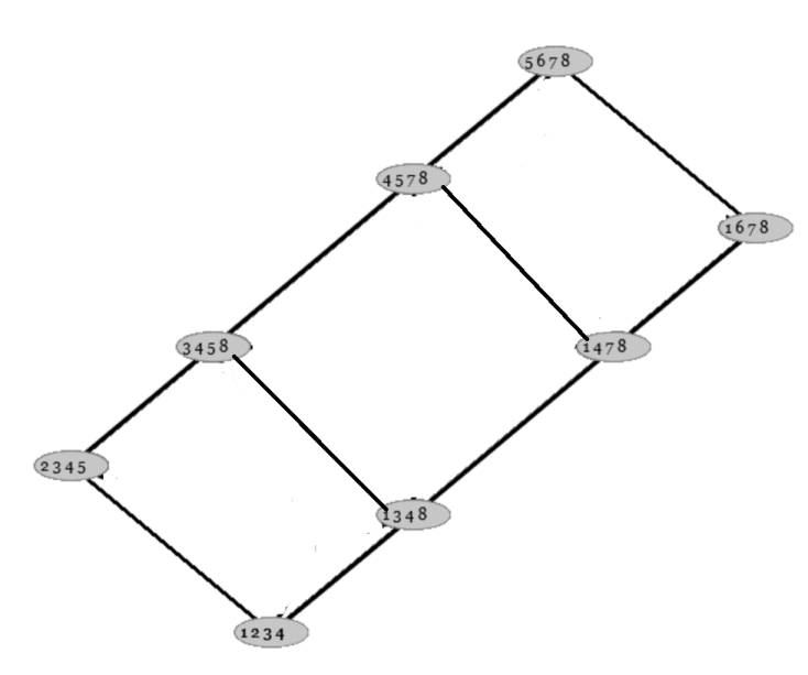
| Interior Size | Exchange Graph Orders | Exchange Graphs |
| 0 | 1 | A |
| 1 | 1, 2 | A, B |
| 2 | 1, 2, 3, 4, 5 | A, B, C, D, B B |
| 3 | 1, 2, 3, 4, 5, 6, 7, 8, 10, 14 | A, B, C, D, E, F, G, H, I, |
| B C, B B B, B D | ||
| 4 | 1, 2, 3, 4, 5, 6, 7, 8, 9, | A, B, C, D, E, F, G, H, I, J, K, L, M, N, |
| 10, 11, 12, 13, 14, 15, 16, 17 | O, P, Q, R, S, T, U, V, W, X, Y, Z1, Z2, | |
| 19, 20, 25, 26, 28, 34, 42 | Z3, Z4, Z5, Z6, B C, B B B, B D, | |
| B E, B G, B F, B H, B I, | ||
| B B B B, B B C, B B D | ||
| C C, D D |
We have the following two results:
Theorem 3.31.
The information is Table 3.1 is true.
Theorem 3.32.
The information in Table 3.2 is true.
| Co-dimension | -Constant Graph Orders | -Constant Graphs |
| 0 | 1 | A |
| 1 | 1, 2 | A, B |
| 2 | 1, 2, 3, 4, 5 | A, B, C, D, B B |
| 3 | 1, 2, 3, 4, 5, 6, 7, 8, 10, 14 | A, B, C, D, E, F, G, H, I, |
| B C, B B B, B D |
In Section 6, we present the following conjecture on a bound for the maximal order of an exchange graph with a given interior size:
Conjecture 3.33.
For any , the maximum possible order of an exchange graph with interior size is the Catalan number (using the convention that , , and ).
In Section 7, we consider very-mutation-friendly exchange graphs in the special cases of cycles and trees. We fully characterize the very-mutation-friendly exchange graphs that are trees. We require the following equivalence classes:
Definition 3.35.
We define to be the equivalence class with the permutation which is defined as follows:
-
•
For , we have .
-
•
For , we let be a permutation on defined as follows:
Theorem 3.36.
Any very-mutation-friendly exchange graph that is a tree must be a path. For an integer , a very-mutation-friendly exchange graph with interior size is a path if and only if it is a part of the equivalence class (path with vertices).
We also fully characterize the equivalence classes of very-mutation-friendly exchange graph with interior size that are single cycles.
Theorem 3.37.
If a very-mutation-friendly exchange graph is a single cycle, then it must have , , , or vertices. If is prime and very-mutation friendly, then must be part of the equivalence class with (cycle with vertex), with (cycle with vertices), or with (cycle with vertices). If is very-mutation-friendly and not prime, then must be a part of the equivalence class with (cycle with vertices).
4. Proof of Theorem 3.28 and Corollary 3.29
Theorem 3.28 is an isomorphism between applicable -constant graphs and exchange graphs. Corollary 3.29 is a special case of Theorem 3.28 in the case of where we show that the applicable condition is no longer necessary.
One direction of the proof of Theorem 3.28 is easy. It is clear that an exchange graph with interior size is isomorphic to the applicable -constant graph which has co-dimension . This proves that the set of possible applicable -constant graphs of co-dimension contains an isomorphic copy of the set of possible exchange graphs with interior size . In this section, we prove the other direction of Theorem 3.28: namely, that every applicable -constant graph is isomorphic to an exchange graph with appropriate interior size. We also prove Corollary 3.29.
In Section 4.1, we introduce with some modifications the approaches of Oh, Postnikov, and Speyer [9, Section 9] as well as Danilov, Karzanov, and Koshevoy [2] involving domains inside special weakly separated collections. In Section 4.2, we construct the machinery of interior-reduced plabic graphs and plabic tilings. In Section 4.3, we construct a decomposition set of a Grassmann necklace. In Section 4.4, we construct adjacency graphs and clusters. In Section 4.5, we prove a special case of Theorem 3.28. In Section 4.6, we use this to prove Theorem 3.28 in the general case. In Section 4.7, we show that all -constant graphs with co-dimension 4 are applicable, which when applied to Theorem 3.28, proves Corollary 3.29.
4.1. Domains inside and outside of cyclic patterns
We introduce with some modifications the approaches in [9] and [2] regarding domains inside non self-intersecting closed curves. Fix unit vectors in the upper half-plane, so that go in this order clockwise around the origin and are -independent. Define:
A subset is identified with the point in .
Now, suppose we have a weakly separated collection of subsets of equal size such that (where indices are considered modulo ). Then we call a sequence. Note that might have repeated subsets. We can associate with a clockwise-oriented piecewise linear closed curve obtained by concatenating the line-segments connecting consecutive points and for .
We consider sequences with the following additional constraint on :
Definition 4.1.
We call a closed curve prong-closed if is the concatenation of curves , , and that satisfy the following conditions:
-
(1)
The curve is a clockwise-oriented non self-intersecting closed curve.
-
(2)
The intersection is a single point .
-
(3)
satisfies one of the following:
-
•
-
•
or the following conditions hold:
-
(a)
is a non self-intersecting open curve,
-
(b)
has an endpoint at ,
-
(c)
has an endpoint at a point in the interior of ,
-
(d)
and .
-
(a)
-
•
We also impose the following constraints on the sequence . Sequences that satsify certain constraints involving weak separation are called generalized cyclic patterns [2]. We consider the following variant of a generalized cyclic pattern:
Definition 4.2.
A quasi-generalized cyclic pattern is a sequence of subsets of where such that
-
(1)
is weakly separated,
-
(2)
the sets in all have the same size,
-
(3)
and
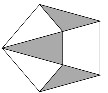
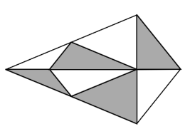
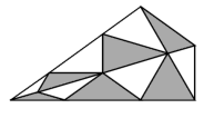
We show two examples of quasi-generalized cyclic patterns such that is prong-closed.
Example 4.3.
Example 4.4.
For an quasi-generalized cyclic pattern such that the curve is prong-closed, let
Remark 4.5.
We describe how to decompose into two pure domains: and . Let be the curve obtained by concatenating and . Then, by definition, we know that subdivides into two closed regions and such that
Then we let
and
4.2. Interior-Reduced Plabic Graphs
We construct the interior-reduced plabic tiling machinery that is helpful in proving Theorem 3.28.
Consider a plabic tiling of a maximal weakly separated collection . Take a sequence of subsets . We call the boundary curve. Consider the sub-plabic tiling consisting of the sets and faces in the plabic tiling of on and within . Suppose that
-
(1)
The boundary curve is prong-closed,
-
(2)
and there do not exist with such that there is a face containing both and in the aformentioned sub-plabic tiling.
Then we call the sub-plabic tiling together with the boundary curve an interior-reduced plabic tiling.
Suppose that there is an interior-reduced plabic tiling that consists of sets of the weakly separated multi-collection (that may have repeated subsets as permitted by ). We omit the phrase “multi” for the remainder of the paper. Then, we denote the interior-reduced plabic tiling of as . Let the sequence of subsets on the boundary be . We let be with the set labels removed.
We now define the interior-reduced plabic graph to be the dual plabic graph (without strand labels) of with the following alteration: Suppose that has repeated elements so that is nonempty. For every two quasi-adjacent sets and connected by , consider the faces in that contain both and . Consider the dual vertices of these faces in the dual plabic graph. If there is only one such vertex, then we split this vertex into two vertices by the move (M2). Now, we let the two vertices be and . We make and into boundary vertices as follows: For , consider the strand that goes from to . We break this strand into two strands so that the first strand ends at and the second strand begins at .
In the case that , we omit the subscripts.
We consider the following examples:
Example 4.6.
Example 4.7.
We prove the following property of interior-reduced plabic graphs:
Proposition 4.8.
Every interior-reduced plabic graph is a reduced plabic graph without strand labels.
Proof.
We consider the interior-reduced plabic graph . First, notice that the condition (2) in the definition of an interior-reduced plabic tiling guarantees that the each boundary vertex of will only have one notch coming out of it on the outside. This means that is a plabic graph. Suppose that we label the strands of the in clockwise order. It suffices to prove that these strands satisfy the properties of a reduced plabic graph. We know that this is true, because the strands of are contained in the strands of the reduced plabic graph of (up to breaking and relabeling). ∎
Notice that the sequence of sets on the boundary curve of an interior-reduced plabic tiling form a modified Grassmann-like necklace which is defined as follows:
Definition 4.9.
Let be a quasi-generalized cyclic pattern. We call a modified Grassmann-like necklace if the following properties are satisfied:
-
(1)
The curve is prong-closed.
-
(2)
There is no such that (where indices are modulo ) and the integers are cyclically ordered.
Remark 4.10.
It follows from the definition that
We associate modified Grassmann-like necklaces with weakly separated multi-collections.
Definition 4.11.
Let be a modified Grassmann-like necklace contained in a maximal weakly separated collection . Then, we define the -enclosed collection of to be
where repeated subsets in continue to be repeated subsets in .
Remark 4.12.
Notice that is always an interior-reduced plabic tiling. We thus know that for a fixed maximal weakly separated collection , the -enclosed collections are in bijection with the interior-reduced plabic tilings/graphs of .
We show two examples of -enclosed collections.
Example 4.13.
Example 4.14.
Now, consider a modified Grassmann-like necklace . Suppose that is contained in a maximal weakly separated collection . We map to a Grassmann necklace in such a way that is independent of choice of . We call the of . We define the decorated permutation associated to as follows. Suppose that . Suppose that has -strands such that starts at the face directly clockwise from the subset . If ends at the face directly clockwise from the subset , then we set . Notice that (and thus the values ) are independent of the choice of maximal weakly separated collection .
We show two examples:
Example 4.15.
Suppose that is defined as in Example 4.13. Then, the relabeled Grassmann necklace is in the equivalence class containing the decorated permutation .
Example 4.16.
If is defined as in Example 4.14, then the relabeled Grassmann necklace is in the equivalence class containing the decorated permutation .
Now, we define the bijective mapping function that sends each -enclosed collection to a maximal weakly separated collection in . In , for each , we label the strand in with the number . Now, we label the sets using these new strand labels. Let this maximal weakly separated collection in be . The function takes to .
We show how to obtain from . We relabel the strands of , replacing the label of the strand that is labeled in with the label of the strand in for . We label the sets and to each set, add the elements of (the elements common to all of the sets in the modified Grassmann-like necklace). This recovers the -enclosed collection .
We say that and if the relabeled Grassmann necklace of the modified-like Grassmann necklace that forms the boundary of is in the same equivalence class as the relabeled Grassmann necklace of the modified-like Grassmann necklace that forms the boundary of . Notice that and if can be transformed into through a sequence of rotations, reflections, and color flipping operations.
We now relate the plabic tilings of -enclosed collections with plabic tilings of maximal weakly separated collections over (the relabeled Grassmann necklace of ). This gives us an isomorphism between certain -constant graphs and certain exchange graphs.
Lemma 4.17.
Consider a maximal weakly separated collection over a Grassmann necklace . Consider a modified-like Grassmann necklace over the relabeled Grassmann necklace and the -enclosed collection . Then, we have that
and
where repeated subsets in are deleted so that contains at most one of each subset.
Proof.
Notice that first equation follows from the bijective mapping function between -enclosed collections and maximal weakly separated collections over a Grassmann necklace and the definition of interior-reduced plabic tilings. Since square moves will have the same effect on the two plabic tilings, up to relabeling, it also follows that the second equation holds. ∎
4.3. Direct Product
We define and prove some results regarding the decomposition set and direct product of Grassmann necklaces.
We define the following notion of decomposition. Let be a Grassmann necklace and be the associated prong-closed curve. We construct the following complex: begin with and add an edge between the embeddings of and if and only if and are quasi-adjacent. Then, this complex will look like a graph with many cycles (some complete graphs) glued together and each cycle (or complete graph) will itself be a modified-like Grassmann necklace. Suppose there are such cycles (or complete graphs). We define the decomposition set to be
where each is one of the aforementioned modified-like Grassmann necklaces. We define the relabeled decomposition set to be
where is the relabeled Grassmann necklace of .
Remark 4.18.
Notice that
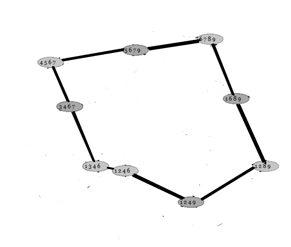
Example 4.19.
Consider the Grassmann necklace
. The decomposition complex of is shown in Figure 14. Notice that contains the following three modified-like Grassmann necklaces:
We now define notions related to the direct product of Grassmann necklaces.
Definition 4.20.
Given a Grassmann necklace with associated permutation on and with associated permutation on , we let the glued Grassmann necklace have decorated permutation on defined as follows:
Example 4.21.
Let have decorated permutation and have decorated permutation . Then has decorated permutation .
The glued Grassmann necklace can be obtained by gluing together the plabic tilings of and along the edge between and , and and . In fact, this idea can be extended to the maximal weakly separated collections over these Grassmann necklaces. Let be in and let be in . Then let be the maximal weakly separated collection in obtained by gluing and along that same edge.
Example 4.22.
We now prove the following proposition about glued Grassmann necklaces:
Proposition 4.23.
Given a Grassmann necklace with associated permutation on and a Grassmann necklace with associated permutation , we have that
and
Proof.
Notice that
It follows that
Furthermore, the maximal weakly separated collection can be mutated into if and only if can be mutated into in or can be mutated into . This means that ∎
We prove the following lemma involving direct products and decomposition sets.
Lemma 4.24.
For a Grassmann necklace , the following is true:
If is mutation-friendly, then each is mutation-friendly for . For any collection of exchange graphs , ,,, there exists a Grassmann necklace such that
and
If all of the are mutation-friendly, then there exists such a that is mutation-friendly.
Proof.
For , we let be the mapping function for and be in . Then we define to be the maximal weakly separated collection in such that for . Notice that
It is clear that can be mutated into in one square move if and only if can be mutated into for some and for all This shows that
Given a collection of Grassmann necklaces , a repeated application of Proposition 4.23 shows that there exists an isomorphic exchange graph with the appropriate interior size.
Notice that the mutation-friendly conditions hold since
-
(1)
The decomposition set of a mutation-friendly Grassmann necklace consists of modified-like Grassmann necklaces over relabeled Grassmann necklaces that are mutation-friendly.
-
(2)
The glued Grassmann necklace of two mutation-friendly Grassmann necklaces is also mutation-friendly.
∎
This motivates the definition of a prime Grassmann necklace:
Definition 4.25.
We call a Grassmann necklace prime if its decomposition set has only one element. We also call the corresponding exchange graph prime.
The definition of the operation on decorated permutations allows us to characterize the decorated permutations of prime Grassmann necklaces:
Corollary 4.26.
If a Grassmann necklace has decorated permutation , it is not prime if there exists a cyclically considered interval such that and .
4.4. Adjacency Graphs and Clusters
We define and prove results relating to adjacency.
We define the adjacency graph as follows:
Definition 4.27.
Let be a maximal weakly separated collection over a Grassmann necklace . Let be a weakly separated collection contained in such that . Then, we define the adjacency graph as follows:
-
•
The vertex set of is .
-
•
The vertices and are connected by an edge if and only if they are adjacent in .
Example 4.28.
In the case that , we denote the adjacency graph as .
We prove the following proposition regarding the adjacency graphs of prime Grassmann necklaces.
Proposition 4.29.
For a given Grassmann necklace , the adjacency graph is either connected for all or not connected for any . In particular, is connected if and only if is a prime Grassmann necklace.
Proof.
For , we let
We will show that
First, notice that for , we have that
so and do not share any of the same vertices. Also, notice that and both consist of the sets in the weakly separated collection . Furthermore, notice that given sets and where , we have that is not adjacent to in , so there are no edges between vertices in and for .
Also, we know that is connected for all This means that is connected if and only if , a condition independent of and equivalent to the prime condition on . ∎
We define an adjacency grouping using the notion of an adjacency graph.
Definition 4.30.
Let be a maximal weakly separated collection over a Grassmann necklace . Let be a weakly separated collection contained in such that . Then, we define the to be the partition of generated by the connected components of .
Suppose that is a set of weakly separated collections. We denote these collections by for .
Example 4.31.
We define and as in Example Then we have the following:
We define the notion of a weakly separated collection being connected in a maximal weakly separated collection.
Definition 4.32.
Let be a maximal weakly separated collection over a Grassmann necklace . Let be a weakly separated collection contained in such that . Suppose that has only one element. Then, we call the weakly separated collection . Suppose also that is applicable. Then, we call the weakly separated collection .
Let be a weakly separated collection over and let be in . Notice that if is very-connected in , then must be very-connected in . We say that is reverse-very-connected over if is very-connected for any .
We define an adjacency collection:
Definition 4.33.
Let be a maximal weakly separated collection over a Grassmann necklace . Let be a set in . We call the adjacency collection be the collection of all elements in adjacent to .
We use the notion of an adjacency collection to define an adjacency cluster:
Definition 4.34.
Let be a maximal weakly separated collection over a Grassmann necklace . Let be a weakly separated collection contained in such that . Then, we define the of to be
Example 4.35.
We define as in Example 3.9. We consider the following two weakly separated collections contained in :
Then is equivalent to the weakly separated collection in Example 4.7 (with repeated subsets deleted so that contains at most one of each set) and is equivalent to the weakly separated collection in Example 4.6.
4.5. Isomorphism in the case of Very-Connected Weakly Separated Collections
We consider Theorem 3.28 in the case where is reverse-very-connected over . We start with the following lemma:
Lemma 4.36.
Let be a maximal weakly separated collection over a Grassmann necklace . Let be a very-connected weakly separated collection in . Then there exists a unique interior-reduced plabic tiling consisting exactly of the sets in (though there might be repeated sets on the boundary curve) and with interior sets exactly equal to . In fact, this interior-reduced plabic tiling must be
We use the following definition in the proof of Lemma 4.36.
Definition 4.37.
Let be a maximal weakly separated collection, and let be very-connected in . Consider the adjacency graph . A reduction is a connected weakly separated collection of such that and
Remark 4.38.
Notice that a reduction always exists.
We use the notion of a reduction to prove Lemma 4.36.
Proof of Lemma 4.36.
The uniqueness of such an interior-reduced plabic tiling is easy to see. To prove that is an interior-reduced plabic tiling and has interior sets equal to , we induct on the size of . The base case is . Notice that looks like a polygon with boundary sets and one set in the interior for some . This is an interior-reduced plabic tiling over a relabeled Grassmann necklace with associated permutation in the equivalence class of the permutation below: for even and for odd , shifted mod as necessary.
We consider an example.
Example 4.39.
Let . Then Figure 17 shows the plabic tiling of the relabeled Grassmann necklace (with associated decorated permutation
For all such that and is any very-connected weakly separated collection in a maximal weakly separated collection , we assume that is an interior-reduced plabic tiling and has interior sets equal to . We will show that for every such for , we have that is an interior-reduced plabic tiling and has interior sets equal to . By the induction hypothesis, we know that is an interior-reduced plabic tiling and has interior sets equal to . We know that the set must be one of the sets on the boundary curve of . Notice that
We add the sets in to and add the set to the interior of to obtain .
We consider two examples of this.
Example 4.40.
Example 4.41.
Let , , , , and be defined as in Example 4.35. It is easy to see that (shown in Example 4.7) is an interior-reduced plabic tiling and satisfies the desired properties. Notice that . the associated interior-reduced plabic tiling is shown there. Notice that The adjacency cluster of contains , , , and . All of these sets are contained in . Thus the set simply needs to be added to the interior. It is easy to see that (shown in Example 4.6) is an interior-reduced plabic tiling and satisfies the desired properties.
The applicable constraint ensures that adding the sets of to results in a valid interior-reduced plabic tiling. Specifically, the boundary of continues to be a prong-closed curve with no disconnected sets in the interior after the addition of the sets in (see Remark 4.42 for discussion). The fact that only sets adjacent to were added ensures that condition (2) of Definition 4.9 continues to be satisfied. It is thus clear that the resulting process results in the interior-reduced plabic tiling as desired. ∎
Remark 4.42.
Roughly speaking, the applicable constraint prevents the addition of the faces in from “entrapping” any additional subsets on the boundary curve of . That is, no subsets on the boundary curve of (besides ) will become disconnected from the rest of the boundary in the plabic tiling of .
This is illustrated in the following example:
Example 4.43.
Consider , , , and as in Example 3.10. Consider the following weakly separated collections:
Notice that . Figure 20 shows that is an interior-reduced plabic graph with boundary that is a prong-closed curve as expected. Notice that the addition of is not possible, because it would disconnect the set from the rest of the boundary. As a result, the boundary would no longer be a prong-closed curve as required.
For a reverse-very-connected weakly separated collection over a Grassmann necklace , we define the following:
In the case , we call this set .
Lemma 4.44.
Consider a reverse-very-connected weakly separated collection over a Grassmann necklace . Let be in . Let be the relabeled Grassmann necklace of the interior-reduced plabic graph of . Then, we have the following:
If is mutation-friendly, then is mutation-friendly.
Proof.
We first prove the first equation. By Lemma 4.36, we know that forms an interior-reduced plabic graph with interior sets of exactly equal to the sets in . Notice that
is equal to and thus congruent to by Lemma 4.17.
The second equation follows from the fact that square moves have the same effect on corresponding plabic tilings. This also implies that the mutation-friendly condition holds. ∎
4.6. Proof of Theorem 3.28
We first prove the following lemma:
Lemma 4.45.
Given an applicable -constant graph and maximal weakly separated collection , we have
If is mutation-friendly, then each is mutation-friendly.
Proof.
Let be . Let be in for . We define
Notice that
Furthermore, the weakly separated collection can be mutated into if and only if can be mutated into for some and for . This means that
and that the mutation-friendly condition holds. ∎
Proof of Theorem 3.28.
Consider an applicable -constant graph and a maximal weakly separated collection . We prove that is isomorphic to an exchange graph with interior size By Lemma 4.45, we know that is isomorphic to the direct product of the -constant graphs for (where the mutation-friendly condition holds). Notice that is a very-connected weakly separated collection in for . By Lemma 4.44, we know that each is isomorphic to an exchange graph with interior size (where the mutation-friendly condition holds). Let this exchange graph be . Then, we know that
By Lemma 4.24, we know that is isomorphic to an exchange graph with interior size
where the mutation-friendly condition also holds. ∎
4.7. Proof of Corollary 3.29
We show show Corollary 3.29 follows from Theorem 3.28. In order to do so, we first prove that the following for -constant graphs with small co-dimension:
Lemma 4.46.
Every -constant graph of co-dimension is applicable.
Proof.
Consider a -constant graph that is not applicable. This means there exists such that no set in or is quasi-adjacent to . First, this means that is not in . Now, consider a maximal weakly separated collection . Notice that there must be at least sets in that are quasi-adjacent to . Hence, we know that the co-dimension of . ∎
5. Proof of Theorem 3.1 and Theorem 3.2
We now characterize exchange graphs with interior size and their associated decorated permutations. We also provide a characterization of all -constant graphs of co-dimension . In Section 5.1, we prove properties of mutation-friendly Grassmann necklaces that we require to prove Theorem 3.1 and Theorem 3.2. In Section 5.2, we prove Theorem 3.1. In Section 5.3, we prove Theorem 3.2.
5.1. Mutation-Friendly Grassmann Necklaces
We first prove the following fact of -constant graphs of very-mutation-friendly graphs which we use to prove our later properties.
Proposition 5.1.
Let be a very-mutation-friendly Grassmann necklace with interior size . Consider the weakly separated collections
using the notation in Definition 3.14 applied to and adding the weakly separated collection . Let be a maximal weakly separated collection in . Let be an integer such that . Let be a weakly separated collection in . Suppose that has boundary curve with relabeled Grassmann necklace . Then is very-mutation-friendly.
Proof.
We split the proof into two cases: and .
Case 1: . Consider the weakly separated collections
| (2) |
First, notice that . For , we want to show that is mutation-friendly and applicable. This follows directly from the fact that is applicable and mutation-friendly. We know that deleting repeated weakly separated collections in gives us the desired requirement for Definition 3.14.
Case 2: . Let be the set at the point in using the notation in Definition For , let be the weakly separated multi-collection consisting of and an additional copy of the set . Consider the resulting weakly separated collections
| (3) |
First, notice that . For , we want to show that is mutation-friendly and applicable. This follows directly from the fact that is applicable and mutation-friendly. We know that deleting repeated weakly separated collections in gives us the desired requirement for Definition 3.14. ∎
We prove the following bound on the number of sets in a very-mutation-friendly Grassmann necklaces as a function with interior size:
Lemma 5.2.
Let be a very-mutation-friendly, prime Grassmann necklace. If , then .
Remark 5.3.
This lemma gives a necessary but not sufficient bound on the size of a very-mutation-friendly Grassmann necklace.
Example 5.4.
Consider the permutation . Let be the Grassmann necklace which corresponds to . It can verified that is prime. Notice that and . This means that satisfies the inequality in Lemma 5.2. However, every maximal weakly separated collection in contains the set which is not in . Thus, is not mutation-friendly.
Proof of Lemma 5.2.
Let . We proceed by induction on .
For the base case, we consider very-mutation-friendly Grassmann necklaces such that . Notice that must be part of the equivalence class of This means that as desired.
Assume that for all very-mutation-friendly, prime Grassmann necklaces with interior size such that , we have that . Now, consider a very-mutation-friendly, prime Grassmann necklace with interior size . Consider the weakly separated collections:
using the notation in Definition 3.14 applied to . We define the set as follows:
By Definition 3.14, we know that is applicable and mutation-friendly. Consider such that is mutatable in . Suppose that the adjacency grouping is a partition containing weakly separated collections that we call For , suppose that has boundary curve with relabeled Grassmann necklace .
By Proposition 5.1, we have that is very-mutation-friendly. Thus by the induction hypothesis, we have that
| (4) |
Also, notice that for all , we have that
| (5) |
We also have that
| (6) |
For any , we have that
| (7) |
We can obtain from the set and from and for as follows:
| (8) |
where in the case of multi-collections, duplicate copies of all sets are deleted so that does not have any repeated sets.
Consider the curve corresponding to . We split the remainder our proof into two cases: for some and for all .
Case 1: for some . By , since no set in can be on , we know that must be on . This means that is in the interior of the closed curve . This implies that . By the , we have that . We also know that
Hence we have that
Applying (8) and thus gives us that
as desired.
We prove the following lemma involving the decomposition set of a very-mutation-friendly Grassmann necklace.
Lemma 5.5.
Given a very-mutation-friendly Grassmann necklace , the relabeled Grassmann necklace of every Grassmann necklace in the decomposition set is very-mutation-friendly.
Proof.
We use the notation from Proposition Let be a maximal weakly separated collection in . Notice that
Thus, the desired result follows from Proposition 5.1. ∎
We also prove the following lemma involving very-mutation-friendly exchange graphs of small interior size.
Lemma 5.6.
Any exchange graph with interior size is isomorphic to a very-mutation-friendly exchange graph with interior size .
We use the following propositions in our proof:
Proposition 5.7.
For every mutation-friendly -constant graph of co-dimension , there exists a weakly separated collection such that and is mutation friendly with co-dimension .
Proof.
We obtain as follows: Fix a maximal weakly separated collection . For each set , let be the minimum path length in from to reach a that does not contain . Consider such that is maximal. Then, let . ∎
Proposition 5.8.
All mutation-friendly exchange graphs with interior size are very-mutation-friendly.
Proof.
We now prove Lemma 5.6.
Proof of Lemma 5.6.
Suppose that is mutation-friendly with interior size . Then by Proposition 5.8, we know that is very-mutation-friendly as desired.
Suppose that with interior size is not mutation-friendly and . By definition, we know that and . We also know that is mutation-friendly. By Theorem 5.6, we know that is isomorphic to a mutation-friendly exchange graph with interior size . By Proposition 5.8, we know that is very-mutation-friendly with interior size as desired. ∎
5.2. Proof of Theorem 3.31
We can decompose the set of exchange graphs for interior size for into sets of prime, mutation-friendly exchange graphs as follows:
Lemma 5.9.
For any nonnegative integer , the set of exchange graphs with interior size is exactly:
where each is a prime, very-mutation-friendly exchange graph.
Proof.
Consider an exchange graph with interior size where . By Lemma 5.6, we know that is isomorphic to a very-mutation-friendly exchange graph where is a Grassmann necklace with interior size . By Lemma 4.24 and Lemma 5.5, we know that is isomorphic to a direct product in the above form.
Conversely, suppose that we have a direct product in the above form. By Lemma 4.24, we know that there exists a Grassmann necklace with exchange graph with the desired interior size isomorphic to the desired direct product. ∎
Proof of Theorem 3.31.
By Theorem 5.9, the set of exchange graphs with interior size for is reduced to computing all prime mutation-friendly exchange graphs with interior size . Let be the Grassmann necklace of any prime, very-mutation-friendly exchange graph with interior size . If , by Theorem 5.2, we know that . If , it is easy to see that corresponds to the decorated permutation . This reduces proving the results in Table 3.1 to a finite computation, which we executed using a computer program. The results of this computer program are shown in Table A.1, which shows all equivalence classes of prime, mutation-friendly Grassmann necklaces and their corresponding exchange graphs. ∎
5.3. Proof of Theorem 3.32
Proof of Theorem 3.32.
By Corollary 3.29, we know that the set of -constant graphs of co-dimension for is equivalent to the set of exchange graphs with interior size . In the case that , it is easy to see that the only possible -constant graph is a path with one vertex. The results in Table 3.2 follow from Theorem 3.31. ∎
6. Explanation of Conjecture 3.33
Conjecture 3.33 involves the maximum order of an exchange graph of a given interior size. We denote by the maximum possible order of an exchange graph with interior size . Conjecture 3.33 is partially motivated by the following:
Proposition 6.1.
For any , a lower bound on is the Catalan number (where ).
Proof.
We can construct an exchange graph with interior size that has order by taking This correspond to triangulations of a -gon. ∎
We now discuss further motivation for Conjecture 3.33:
Remark 6.2.
Theorem 3.31 proves Conjecture 3.33 for . The results in Table A.1 motivates us to hypothesize that the only Grassmann necklaces with interior size and order are Grassmann necklaces in the equivalence class of
In the case of triangulations, the interior size is equal to the number of mutatable subsets at each step. For other Grassmann necklaces, the interior size is greater than the number of mutatable sets at some steps, since some interior sets are immutatable in some maximal weakly separated collections.
We also note some consequences of Conjecture 3.33:
7. Proof of Theorem 3.37 and Theorem 3.36
Theorem 3.37 and Theorem 3.36 provide a full characterization of very-mutation-friendly exchange graphs in the special cases of cycles and trees. In Section 7.1, we prove relevant properties of mutation-friendly exchange graphs as well as an important property of Grassmann necklaces in . In Section 7.2, we prove Theorem 3.36. In Section 7.3, we prove Theorem 3.37.
7.1. Important Properties of Mutation-Friendly Exchange Graphs and
In Section 7.1.1, we discuss relevant properties involving cycles and -constant graphs of mutation-friendly exchange graphs. In Section 7.1.2, we discuss an important property that relates the exchange graphs of Grassmann necklaces in with the exchange graphs of Grassmann necklaces in .
7.2. Mutation-Friendly Exchange Graphs
We prove the following lemma involving the existence of a cycle in mutation-friendly exchange graphs:
Lemma 7.1.
Given a mutation-friendly, not prime exchange graph with interior size , we know that there exists a -constant graph of co-dimension that is a cycle with vertices.
Proof.
By Lemma 4.24, we know that a not prime exchange graph with interior size is either isomorphic to a prime exchange graph and is not mutation-friendly or has a -constant graph of co-dimension that is a cycle with vertices. The result follows. ∎
We also prove the existence of a cycle in certain applicable, mutation-friendly -constant graphs.
Lemma 7.2.
Let be an exchange graph and let be not reverse-very-connected over . If is applicable and mutation-friendly, then contains a cycle of length .
Proof.
Let be not reverse-very-connected over and suppose that is applicable. Let be in . By definition, we know that
Since is mutation-friendly, the desired result follows from Lemma 4.45. ∎
We also prove the following lemma involving the -constant graphs of very-mutation-friendly exchange graphs:
Lemma 7.3.
Given a very-mutation-friendly exchange graph with interior size , there exists a weakly separated collection over such that the -constant graph is mutation-friendly, has co-dimension , and is isomorphic to a very-mutation-friendly exchange graph of co-dimension .
We require the following proposition in the proof:
Proposition 7.4.
If the Grassmann necklaces , , …, are very-mutation-friendly, then is very-mutation-friendly.
Proof.
Let . WLOG, for each , assume that . Let be the mapping function that takes to . Suppose has interior size . that since is very-mutation-friendly, there exists a maximal weakly separated collection and weakly separated that satisfy:
such that is applicable and mutation-friendly for .
We construct a sequence of weakly separated collections over as follows. For , if , then
This satisfies the requirements of Definition 3.14. ∎
Proof of Lemma 7.3.
Let using the notation in Definition 3.14. By definition, we know that is mutation-friendly and applicable. Suppose that has weakly separated collections. Let be the relabeled Grassmann necklace of the boundary curve of
for . Then by Proposition 5.1, we know that is very-mutation-friendly. By Lemma 4.24, we know that
By Proposition 7.4, we know that is also very-mutation-friendly. By Lemma 4.44, we know that
as desired. ∎
7.3. Equivalence Classes
We use the following notation to discuss .
Consider . Figure 21 shows an element of for . Note that the adjacency graph is a path with vertices for all . Denote the sets in the adjacency graph, , ,.., (in order from left to right along ). The exchange graph is a path with vertices. We label the maximal weakly separated collections in as , ,, so that
-
(1)
In , the set is the only mutatable set.
-
(2)
In , the set is the only mutatable set.
-
(3)
In for , the sets and are the only mutatable sets.
For , we let be the set in the Grassmann necklace that is adjacent to and not adjacent to for any .
Since for all , we denote the set of plabic tilings (without set labels) as
We prove the following lemma that relates to :
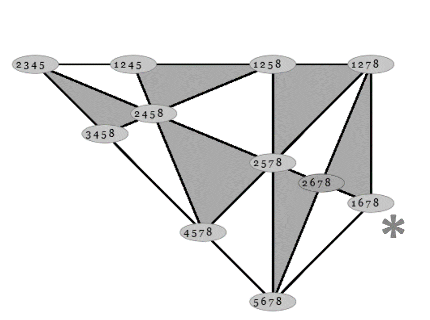
Lemma 7.5.
Let be a very-mutation-friendly exchange graph with interior size . Suppose there is an applicable -constant graph of co-dimension such that is a reverse-very-connected weakly separated collection over and for some . If does not have a -constant graph of co-dimension that is a cycle of length or , then is part of the equivalence class .
Proof.
Assume that very-mutation-friendly exchange graph does not have a -constant graph of co-dimension that is a cycle of length or . By Lemma 7.1, this means that must be prime. Suppose that has an applicable, mutation-friendly -constant graph such that for some . Let be a Grassmann necklace in . Consider such that is mutatable, and let . Then for some .
As we present the general proof, for ease of readability, we also consider the running example where has decorated permutation .
We will show that or . In the example, we consider to be the plabic tiling shown in Figure 22. Assume for sake of contradiction that . In the example, we consider to be the plabic tiling in Figure 23. The set must be adjacent to the sets corresponding to and in . In the example, these are the sets and , the two mutatable faces. (If is not adjacent to a set corresponding to one of them, then the -constant graph will be a cycle of length .) This leaves no spots for .
Hence, or . We know that must be adjacent to the set corresponding to if or corresponding to if . In the example, the set corresponds to as shown in Figure 22. (If is not adjacent to , then the -constant graph will be a cycle of length .) Notice that . However, if , then would be isomorphic to a very-mutation-friendly, prime exchange graph with and interior size , which by Table A.1 is a cycle with vertices. Hence, we know that .
We will now show that must be , that is, it must be in the starred location in Figure 22. Assume for sake of contradiction that corresponds to some other set in the Grassmann necklace besides . Since is mutatable, this means that , which is a contradiction. In the example, suppose that corresponds to the set in Figure 22 and corresponds to the set . Notice that would consist of , , , , , and two more sets adjacent to .
Hence, is in the starred location with . This means that for , where is a Grassmann necklace in . In the example, this is shown in Figure 24. This means that is part of . ∎
7.4. Proof of Theorem 3.36
We prove Theorem 3.36.
Proof of Theorem 3.36.
We notice right away that non prime, very-mutation-friendly exchange graphs are not trees by Lemma 7.1. We prove that prime, very-mutation-friendly exchange graphs with interior size are trees if and only if their Grassmann necklaces are a part of the equivalence class (which yield paths). We proceed by induction on the interior size of .
The base case is when or . By Table A.1, the only possible associated decorated permutations corresponding to are and as desired.
We assume that prime, very-mutation-friendly exchange graphs with interior size are trees if and only if their Grassmann necklaces are a part of the equivalence class (which yield paths). Now, we consider a prime, very-mutation-friendly exchange graph with interior size that is a tree. By Lemma 7.3, we know that there exists a mutation-friendly -constant graph of co-dimension that is isomorphic to a very-mutation-friendly exchange graph with interior size . This graph must be a tree too, so by the induction hypothesis, is part of the equivalence class . By Lemma 7.2, we know that must be reverse-very-connected. Since a tree does not have any cycles, by Lemma 7.5, is part of the equivalence class . ∎
7.5. Proof of Theorem 3.37
We will use the following lemmas in our proof of Theorem 3.37:
Lemma 7.6.
Let be a very-mutation-friendly and prime exchange graph. If , then is not a single cycle.
Proof.
Assume for sake of contradiction that there exists a prime, very-mutation-friendly exchange graph with that is a single cycle. By Lemma 7.3, we know that there exists a mutation-friendly -constant graph of co-dimension that is isomorphic to a very-mutation-friendly exchange graph with interior size . Since is a cycle, must be a path. By Lemma 7.2, we know that must be reverse-very-connected.
Lemma 7.7.
If be a very-mutation-friendly, non-prime exchange graph that is a single cycle, then has vertices and is in the equivalence class with .
Proof.
Consider a very-mutation-friendly, non-prime exchange graph that is a single cycle. By Lemma 7.1, we know that the cycle must have vertices. This is only the case when the graph is a direct product of two paths each with vertices so that the has two Grassmann necklaces. By Lemma 5.5, both and are very-mutation-friendly. By Theorem 3.36, we know that and both must have interior size . Thus, must be in the equivalence class containing the permutation . ∎
We now prove Theorem 3.37.
Proof of Theorem 3.37.
Suppose that is a cycle. First, we consider the case where is prime and very-mutation-friendly. By Lemma 7.6, it suffices to consider . By Table A.1, we know that must be part of the equivalence class (cycle with vertex), (cycle with vertices), or (cycle with vertices).
Now, we consider the case in which is very-mutation-friendly, but not prime. Then by Lemma 7.7, is in the equivalence class (cycle with vertices). ∎
8. Acknowledgments
I would like to thank Miriam Farber (MIT) for her incredibly helpful guidance and insight. I would also like to thank Professor Alexander Postnikov and the MIT-PRIMES program for suggesting this project, and Professor David Speyer for correcting an error in an earlier version of the paper. In addition, I would like to thank Pavel Galashin (MIT) for his helpful software available at http://math.mit.edu/~galashin/plabic.html which was used to generate the plabic tilings and plabic graphs in this paper.
References
- [1] A. Z. B. Leclerc. Quasicommuting families of quantum Pl’́ucker coordinates. Advances in Math. Sciences (Kirillov’s seminar (American Mathematical Society Translations), 181:85–108, 1998.
- [2] V. I. Danilov, A. V. Karzanov, and G. A. Koshevoy. Combined tilings and the purity phenomenon on separated set-systems. ArXiv 1401.6418, 2014.
- [3] Y. Kodama and L. Williams. Combinatorics of kp solitons from the real grassmannian. In B. A. Buan, I. Reiten, and Ø. Solberg, editors, Algebras, Quivers and Representations: The Abel Symposium 2011, pages 155–193. Springer Berlin Heidelberg, Berlin, Heidelberg, 2013.
- [4] S. Oh. Combinatorics of Positroids. FPSAC, 2008.
- [5] A. Postnikov. Total positivity, Grassmannians, and networks. ArXiv math.CO/0609764, 2006.
- [6] J. Scott. Quasi-commuting families of quantum minors. Journal of Algebra, 290:204–220, Aug. 2005.
- [7] J. Scott. Grassmannians and cluster algebras. Proceedings of the London Mathematical Society, 92:345–380, 2006.
- [8] D. E. S. Suho Oh. Links in the complex of weakly separated collections. Journal of Combinatorics, to appear, 2014.
- [9] D. E. S. Suho Oh, Alexander Postnikov. Weak Separation and Plabic Graphs. Proceedings of the London Mathematical Society, pages 721–754, 2015.
Appendix A Full Characterization
Table A.1 is a full characterization of all possible exchange graphs of very-mutation-friendly, prime Grassmann necklaces with interior size 4. There is at least one decorated permutation from each equivalence class, and it is possible that multiple decorated permutations from the same equivalence class are listed.
| Interior Size | Equivalence Class | Exchange Graph Order | Exchange Graph |
| 0 | 312 | 1 | A |
| 1 | 3412 | 2 | B |
| 2 | 365124 | 3 | C |
| 2 | 34512 | 5 | D |
| 3 | 38761254 | 4 | E |
| 3 | 38517246 | 5 | F |
| 3 | 38571426 | 5 | F |
| 3 | 38617425 | 5 | F |
| 3 | 3576214 | 5 | F |
| 3 | 3756124 | 7 | G |
| 3 | 356124 | 10 | H |
| 3 | 345612 | 14 | I |
| 4 | 3(10)98712654 | 5 | J |
| 4 | 37682154 | 6 | K |
| 4 | 3(10)96182574 | 7 | L |
| 4 | 3(10)96815274 | 7 | L |
| 4 | 3(10)97185264 | 7 | L |
| 4 | 397618254 | 7 | L |
| 4 | 36587214 | 7 | M |
| 4 | 3(10)57941628 | 8 | N |
| 4 | 3(10)51829647 | 8 | N |
| 4 | 3(10)51729468 | 8 | N |
| 4 | 3(10)51792648 | 8 | N |
| 4 | 3(10)81794625 | 8 | N |
| 4 | 3(10)69741528 | 8 | N |
| 4 | 395871426 | 8 | N |
| 4 | 397618425 | 8 | N |
| 4 | 379628415 | 8 | N |
| 4 | 36872154 | 8 | N |
| 4 | 3(10)98714625 | 9 | O |
| 4 | 3(10)98741526 | 9 | O |
| 4 | 3(10)96184527 | 9 | O |
| 4 | 3(10)96815427 | 9 | O |
| 4 | 3(10)97185426 | 9 | O |
| 4 | 3(10)97841625 | 9 | O |
| 4 | 3(10)61982574 | 9 | O |
| 4 | 3(10)61895274 | 9 | O |
| 4 | 3(10)81729564 | 9 | O |
| 4 | 375129(10)648 | 9 | O |
| 4 | 39(10)6284517 | 9 | O |
| 4 | 4(10)62895173 | 9 | O |
| Interior Size | Equivalence Class | Exchange Graph Order | Exchange Graph |
|---|---|---|---|
| 4 | 398671254 | 9 | O |
| 4 | 395871264 | 9 | O |
| 4 | 3(10)71985264 | 9 | O |
| 4 | 3(10)58149627 | 9 | P |
| 4 | 395718426 | 9 | P |
| 4 | 35872146 | 9 | P |
| 4 | 395784126 | 10 | Q |
| 4 | 396874125 | 10 | Q |
| 4 | 397681524 | 10 | Q |
| 4 | 48672153 | 10 | Q |
| 4 | 37862145 | 10 | Q |
| 4 | 395618247 | 11 | R |
| 4 | 34768215 | 11 | R |
| 4 | 395681427 | 12 | S |
| 4 | 396178425 | 12 | S |
| 4 | 395178246 | 12 | S |
| 4 | 34761825 | 12 | S |
| 4 | 35871426 | 12 | S |
| 4 | 36872415 | 12 | S |
| 4 | 38761245 | 13 | T |
| 4 | 38671254 | 13 | T |
| 4 | 38571246 | 14 | U |
| 4 | 34(10)1895276 | 15 | V |
| 4 | 3(10)91782564 | 15 | V |
| 4 | 3(10)91784526 | 15 | V |
| 4 | 3(10)96714528 | 15 | V |
| 4 | 3(10)96781524 | 15 | V |
| 4 | 3(10)96784125 | 15 | V |
| 4 | 3(10)97815624 | 15 | V |
| 4 | 3(10)97845126 | 15 | V |
| 4 | 3(10)51789264 | 15 | V |
| 4 | 3(10)51289467 | 15 | V |
| 4 | 3(10)51892674 | 15 | V |
| 4 | 3(10)56794128 | 15 | V |
| 4 | 3(10)61789524 | 15 | V |
| 4 | 3(10)67945128 | 15 | V |
| 4 | 3(10)71895624 | 15 | V |
| 4 | 3(10)71289564 | 15 | V |
| 4 | 365129(10)478 | 15 | V |
| 4 | 34(10)8719562 | 15 | V |
| 4 | 398671425 | 15 | V |
| Interior Size | Equivalence Class | Exchange Graph Order | Exchange Graph |
|---|---|---|---|
| 4 | 348172956 | 15 | V |
| 4 | 346189527 | 15 | V |
| 4 | 396178254 | 15 | V |
| 4 | 38617245 | 15 | W |
| 4 | 38671425 | 15 | W |
| 4 | 34867125 | 16 | X |
| 4 | 34871256 | 16 | X |
| 4 | 3567214 | 17 | Y |
| 4 | 38567124 | 19 | Z1 |
| 4 | 3576124 | 20 | Z2 |
| 4 | 34(10)1789265 | 25 | Z3 |
| 4 | 34(10)1789526 | 25 | Z3 |
| 4 | 34(10)1289567 | 25 | Z3 |
| 4 | 34(10)1892675 | 25 | Z3 |
| 4 | 34(10)1895627 | 25 | Z3 |
| 4 | 34(10)8195672 | 25 | Z3 |
| 4 | 34(10)9815672 | 25 | Z3 |
| 4 | 34(10)6789512 | 25 | Z3 |
| 4 | 34(10)7895612 | 25 | Z3 |
| 4 | 4(10)17895623 | 25 | Z3 |
| 4 | 349178256 | 25 | Z3 |
| 4 | 349781562 | 25 | Z3 |
| 4 | 349678152 | 25 | Z3 |
| 4 | 34718256 | 25 | Z3 |
| 4 | 34617825 | 25 | Z3 |
| 4 | 3467125 | 26 | Z4 |
| 4 | 456123 | 34 | Z5 |
| 4 | 3456712 | 42 | Z6 |
Table A.2 defines the undirected graphs . The table either displays an embedding of the graph or the adjacency information for each vertex.
| Name | Graph [Figure or Adjacency Information] |
|---|---|
| A |
|
| B |
![[Uncaptioned image]](/html/1608.05723/assets/B.png)
|
| C |
![[Uncaptioned image]](/html/1608.05723/assets/C.png)
|
| D |
![[Uncaptioned image]](/html/1608.05723/assets/D.png)
|
| E |
![[Uncaptioned image]](/html/1608.05723/assets/E.png)
|
| F |
![[Uncaptioned image]](/html/1608.05723/assets/F.png)
|
| G |
![[Uncaptioned image]](/html/1608.05723/assets/G.png)
|
| H |
![[Uncaptioned image]](/html/1608.05723/assets/H.png)
|
| I |
| Name (cont.) | Graph [Figure or Adjacency Information] (cont.) |
|---|---|
| J |
![[Uncaptioned image]](/html/1608.05723/assets/J.png)
|
| K |
![[Uncaptioned image]](/html/1608.05723/assets/K.png)
|
| L |
![[Uncaptioned image]](/html/1608.05723/assets/L.png)
|
| M |
![[Uncaptioned image]](/html/1608.05723/assets/M.png)
|
| N |
![[Uncaptioned image]](/html/1608.05723/assets/N.png)
|
| O |
![[Uncaptioned image]](/html/1608.05723/assets/O.png)
|
| P | |
| Q |
![[Uncaptioned image]](/html/1608.05723/assets/Q.png)
|
| R |
| Name (cont.) | Graph [Figure or Adjacency Information] (cont.) |
|---|---|
| R (cont.) | |
| S | |
| T |
| Name (cont.) | Graph [Figure or Adjacency Information] (cont.) |
|---|---|
| U | |
| V | |
| W |
| Name (cont.) | Graph [Figure or Adjacency Information] (cont.) |
|---|---|
| W (cont.) | |
| X | |
| Y |
| Name (cont.) | Graph [Figure or Adjacency Information] (cont.) |
|---|---|
| Y (cont.) | |
| Z1 | |
| Z2 |
| Name (cont.) | Graph [Figure or Adjacency Information] (cont.) |
|---|---|
| Z2 (cont.) | |
| Z3 |
| Name (cont.) | Graph [Figure or Adjacency Information] (cont.) |
|---|---|
| Z3 (cont.) | |
| Z4 |
| Name (cont.) | Graph [Figure or Adjacency Information] (cont.) |
|---|---|
| Z5 |
| Name (cont.) | Graph [Figure or Adjacency Information] (cont.) |
|---|---|
| Z6 |
| Name (cont.) | Graph [Figure or Adjacency Information] (cont.) |
|---|---|
| Z6 (cont.) |