The LPM effect in sequential bremsstrahlung:
4-gluon vertices

Abstract

The splitting processes of bremsstrahlung and pair production in a medium are coherent over large distances in the very high energy limit, which leads to a suppression known as the Landau-Pomeranchuk-Migdal (LPM) effect. In this paper, we continue study of the case when the coherence lengths of two consecutive splitting processes overlap (which is important for understanding corrections to standard treatments of the LPM effect in QCD), avoiding soft-gluon approximations. In particular, this paper completes the calculation of the rate for real double gluon bremsstrahlung from an initial gluon with various simplifying assumptions (thick media; $\hat{q}$ approximation; and large $N_{\rm c}$) by now including processes involving 4-gluon vertices.

I Introduction and Result

When passing through matter, high energy particles lose energy by showering, via the splitting processes of hard bremsstrahlung and pair production. At very high energy, the quantum mechanical duration of each splitting process, known as the formation time, exceeds the mean free time for collisions with the medium, leading to a significant reduction in the splitting rate known as the Landau-Pomeranchuk-Migdal (LPM) effect LP ; Migdal . A long-standing problem in field theory has been to understand how to implement this effect in cases where the formation times of two consecutive splittings overlap.

Let $x$ and $y$ be the longitudinal momentum fractions of two consecutive bremsstrahlung gauge bosons. In the limit $y\ll x\ll 1$, the problem of overlapping formation times has been analyzed at leading logarithm order in refs. Blaizot ; Iancu ; Wu in the context of energy loss of high-momentum partons traversing a QCD medium (such as a quark-gluon plasma). We subsequently developed and implemented field theory formalism needed for the more general case where $x$ and $y$ are arbitrary 2brem ; seq ; dimreg . In this paper, we finally complete the calculation of the effect of overlapping formation times on the differential rate $d\Gamma/dx\,dy$ for double bremsstrahlung from an initial high-energy gluon (with various simplifying assumptions detailed below). The missing element, presented in this paper, is the inclusion of processes involving the 4-gluon vertex.

I.1 What we compute (and what we do not)

The preceding work 2brem ; seq ; dimreg computed all of the interference contributions involving only 3-gluon vertices, which are presented by the diagrams of figs. 1 and 2, which we respectively refer to as “crossed” and “sequential” diagrams. The upper (blue) part of each diagram depicts a contribution to the amplitude and the lower (red) part depicts a contribution to the conjugate amplitude. Only the high energy particles are shown; their (many) interactions with the medium are implicit. (See ref. 2brem for more details.)

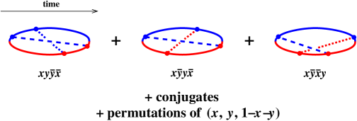
Figure 1: The subset of interference contributions to double splitting previously evaluated in ref. 2brem , the “crossed” diagrams, depicted as amplitudes (blue) sewn together with conjugate amplitudes (red). The dashed lines are colored according to whether they were first emitted in the amplitude or conjugate amplitude. To simplify the drawing, all particles, including bremsstrahlung gluons, are indicated by straight or curved lines. The long-dashed and short-dashed lines are the daughters with momentum fractions $x$ and $y$ respectively. The naming of the diagrams indicates the time order in which emissions occur in the amplitude and conjugate amplitude. For instance, $x\bar{y}y\bar{x}$ means first (i) $x$ emission in the amplitude, then (ii) $y$ emission in the conjugate amplitude, then (iii) $y$ emission in the amplitude, and then (iv) $x$ emission in the conjugate amplitude.

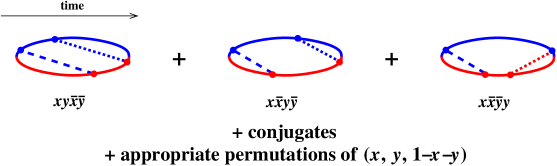
Figure 2: The interference contributions evaluated in ref. seq : the “sequential” diagrams.

In this paper, we will evaluate the remaining contributions, which are the diagrams involving 4-point gluon vertices, shown in figs. 3 and 4. (We will see later, by a symmetry argument, that the $\bar{y}4\bar{x}$ contribution in fig. 3 vanishes.) Once we find the correct normalization of the 4-gluon vertex in our formalism, the evaluation of these diagrams will be a relatively straightforward application of techniques developed in previous papers 2brem ; seq .

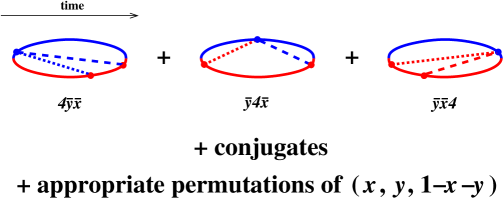
Figure 3: The interference contributions involving a single 4-gluon vertex. The naming conventions are the same as described in the caption of fig. 1 with the addition that “4” indicates a 4-gluon vertex where $x$ and $y$ are emitted simultaneously.

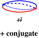
Figure 4: The interference contribution involving two 4-gluon vertices.

As discussed in the preceding work 2brem ; seq , it is possible to set up the formalism in a quite general way that would require both highly non-trivial numerics and a non-trivial treatment of color dynamics to implement, but one can proceed much further analytically by making a few additional approximations. Though the methods we discuss in this paper can be applied more generally, we will follow refs. 2brem ; seq when it comes to explicit calculations, by making the following approximations.

• We will assume that the medium is static, uniform and infinite (which in physical terms means approximately uniform over the formation time and corresponding formation length).

• We take the large-$N_{\rm c}$ limit of QCD to simplify the color dynamics.

• We make the multiple-scattering approximation to interactions with the medium, appropriate for very high energies and also known as the harmonic oscillator or $\hat{q}$ approximation.

In this paper, we focus on completing the calculation of the rate for producing two real bremsstrahlung gluons ($g\to ggg$). We defer to another time the related calculation of the change in the single-bremsstrahlung rate due to virtual corrections. (In the special limiting case $y\ll x\ll 1$, the sum of these real and virtual processes has been worked out in the context of leading parton average energy loss in refs. Blaizot ; Iancu ; Wu and is related to anomalous scaling of the effective medium parameter $\hat{q}$ with energy.)

Finally, as discussed in ref. seq , the double bremsstrahlung rate $d\Gamma/dx\,dy$ by itself includes processes where two single-bremsstrahlung processes are separated by times large compared to their corresponding formation times. In the idealization of an infinite, uniform medium, this causes $d\Gamma/dx\,dy$ to be formally infinite. But what we actually want to know is the correction to double bremsstrahlung due to overlapping formation times,

$$\Delta\,\frac{d\Gamma}{dx\,dy}\equiv\frac{d\Gamma}{dx\,dy}-\left[\frac{d\Gamma}{dx\,dy}\right]_{\rm IMC},$$ (1)

where $[d\Gamma/dx\,dy]_{\rm IMC}$ represents the idealized in-medium “Monte Carlo” result one would obtain based only on the rates for single-bremsstrahlung processes. See the introduction of ref. seq for a detailed explanation. The correction $\Delta\,d\Gamma/dx\,dy$ is finite and only depends on time separations that are $\lesssim$ formation times. The subtraction (1) is an issue relevant only to the the sequential diagram contributions of fig. 2; we will not need to worry about it when evaluating the 4-gluon vertex diagrams of figs. 3 and 4. The subtraction will be relevant only for presenting complete, final results for the double bremsstrahlung rate, which combine all the contributions of figs. 1–4.

I.2 Preview of Results

Numerical results for the total $\Delta\,d\Gamma/dx\,dy$ are shown in fig. 5, which includes all contributions from figs. 1–4. In ref. seq , it was shown that the contribution from crossed and sequential diagrams (figs. 1 and 2) scale as $1/xy^{3/2}$ for $y\ll x\ll 1$, and for this reason it has been convenient to show the result in fig. 5 in units of

$$\frac{C_{\rm A}^{2}\alpha_{\rm s}^{2}}{\pi^{2}xy^{3/2}}\sqrt{\frac{\hat{q}_{\rm A}}{E}}.$$ (2)

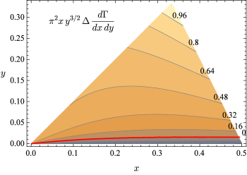
Figure 5: Result for $\pi^{2}xy^{3/2}\,\Delta\,d\Gamma/dx\,dy$ in units of $C_{\rm A}^{2}\alpha_{\rm s}^{2}\sqrt{\hat{q}_{\rm A}/E}$ [which is equivalent to saying the result for $\Delta\,d\Gamma/dx\,dy$ in units of (2)]. Since all three final state particles are gluons and so are identical particles, we only show results for the region $y<x<z\equiv 1{-}x{-}y$. (All other orderings are related by permutation.) The red line shows where the result vanishes, dividing the sub-region of positive corrections from the sub-region of negative corrections. At the apex ($x{=}y{=}\frac{1}{3}$) of the triangular region, $\pi^{2}xy^{3/2}\,\Delta\,d\Gamma/dx\,dy=1.12\,C_{\rm A}^{2}\alpha_{\rm s}^{2}\sqrt{\hat{q}_{\rm A}/E}$.

In comparison to the similar plot in ref. seq , not much has changed: the inclusion of the 4-gluon vertex contributions of figs. 3 and 4 in this paper have had only a small effect on the total. We show the contributions of figs. 3 and 4 individually in figs. 6 and 7. The first of these is numerically negligible compared to the total of fig. 5. (We do not know any qualitative explanation for why it should be so small.) The second (fig. 7) is only a very modest contribution to the total.

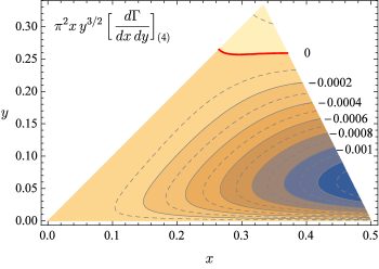
Figure 6: As fig. 5 but only showing the contribution from the diagrams of fig. 3, which are the diagrams with a single 4-gluon vertex. At the apex, $\pi^{2}xy^{3/2}[d\Gamma/dx\,dy]_{(4)}=0.00012\,C_{\rm A}^{2}\alpha_{\rm s}^{2}\sqrt{\hat{q}_{\rm A}/E}$.

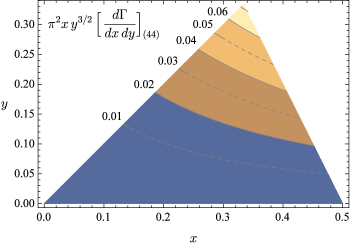
Figure 7: As fig. 5 but only showing the contribution from the diagrams of fig. 4, which are the diagrams with two 4-gluon vertices. At the apex, $\pi^{2}xy^{3/2}[d\Gamma/dx\,dy]_{(44)}=0.072\,C_{\rm A}^{2}\alpha_{\rm s}^{2}\sqrt{\hat{q}_{\rm A}/E}$.

None of the new, 4-gluon vertex contributions to $\Delta\,d\Gamma/dx\,dy$ grow as quickly as (2) for $y\ll x\ll 1$. We find that they instead scale as $1/y^{1/2}$ in this limit.

I.3 Outline and Referencing

In the next section, we show how to calculate the $4\bar{y}\bar{x}$ interference diagram of fig. 3, which will be our canonical example in this paper. Section III then explains how to obtain all of the other diagrams involving 4-gluon vertices. A summary of final formulas is given in section IV, and we offer our brief conclusion in section V. Along the way, some details and cross-checks are relegated to appendices. In particular, for the sake of completeness, we have collected in Appendix D the formulas for crossed and sequential diagrams from refs. 2brem ; dimreg ; seq , so that this paper contains, in one place, all the formulas necessary for implementing the complete calculation of $\Delta\,d\Gamma/dx\,dy$. Also, the integral formula we will derive for $\Delta\,d\Gamma/dx\,dy$ is a complicated expression that is painstaking to implement. In Appendix E, we provide, as an alternative, a relatively simple analytic formula that has been fitted to approximate fig. 5 very well.

In this paper, we will occasionally (in footnotes and appendices) use the author acronym AI as shorthand for Arnold and Iqbal 2brem so that, for example, we may write “AI (5.2)” to refer to eq. (5.2) of ref. 2brem .

II The $4\bar{y}\bar{x}$ diagram

II.1 Starting point

We start with the $4\bar{y}\bar{x}$ diagram shown in fig. 8. In the notation of ref. 2brem , this is

$$\left[\frac{dI}{dx\,dy}\right]_{4\bar{y}\bar{x}}=\left(\frac{E}{2\pi}\right)^{2}\int_{t_{(4)}<t_{\bar{\rm y}}<t_{\bar{\rm x}}} \sum_{\rm pol.}\langle|i\,\overline{\delta H}|{\bm{B}}^{\bar{\rm x}}\rangle\,\langle{\bm{B}}^{\bar{\rm x}},t_{\bar{\rm x}}|{\bm{B}}^{\bar{\rm y}},t_{\bar{\rm y}}\rangle\langle{\bm{B}}^{\bar{\rm y}}|i\,\overline{\delta H}|{\bm{C}}_{34}^{\bar{\rm y}},{\bm{C}}_{12}^{\bar{\rm y}}\rangle\,$$

$$\times\langle{\bm{C}}_{34}^{\bar{\rm y}},{\bm{C}}_{12}^{\bar{\rm y}},t_{\bar{\rm y}}|{\bm{C}}_{34}^{(4)},{\bm{C}}_{12}^{(4)},t_{(4)}\rangle\langle{\bm{C}}_{34}^{(4)},{\bm{C}}_{12}^{(4)}|{-}i\,\delta H|\rangle.$$ (3)

$\langle{\bm{C}}_{34}^{\bar{\rm y}},{\bm{C}}_{12}^{\bar{\rm y}},t_{\bar{\rm y}}|{\bm{C}}_{34}^{(4)},{\bm{C}}_{12}^{(4)},t_{(4)}\rangle$ and $\langle{\bm{B}}^{\bar{\rm x}},t_{\bar{\rm x}}|{\bm{B}}^{\bar{\rm y}},t_{\bar{\rm y}}\rangle$ represent, respectively, the (i) 4-particle evolution in the initial time interval $t_{(4)}<t<t_{\bar{\rm y}}$ in the figure, and (ii) 3-particle evolution of the system in the final interval $t_{\bar{\rm y}}<t<t_{\bar{\rm x}}$. Because of the symmetries of the problem, these have been reduced to effective (i) 2-particle and (ii) 1-particle problems in non-Hermitian two-dimensional quantum mechanics, described by effective transverse coordinates (i) $({\bm{C}}_{34},{\bm{C}}_{12})$ and (ii) ${\bm{B}}$. $\delta H$ represents the piece of the fundamental QCD Hamiltonian associated with the splitting vertices for the high-energy particles (as opposed to the interactions of those high-energy particle with the medium, or the interaction of the medium with itself). So $\langle{\bm{C}}_{34}^{(4)},{\bm{C}}_{12}^{(4)}|\delta H|\rangle$ represents the matrix element for the 4-gluon splitting vertex in fig. 8, appropriately normalized according to the normalization conventions for the states $|{\bm{C}}_{34}^{(4)},{\bm{C}}_{12}^{(4)}\rangle$ and $|\rangle$ given in ref. 2brem .

Figure 8: Labeling conventions for helicities $h_{i}$ and longitudinal momenta $x_{i}$ for the $4\bar{y}\bar{x}$ interference diagram.

Above, ${\bm{C}}_{ij}\equiv({\bm{b}}_{i}-{\bm{b}}_{j})/(x_{i}+x_{j})$ where the ${\bm{b}}_{i}$ are the various transverse positions of the individual particles and $x_{i}$ are their longitudinal momentum fractions (defined as negative for particles in the conjugate amplitude). ${\bm{B}}\equiv{\bm{B}}_{12}={\bm{B}}_{23}={\bm{B}}_{31}$ is defined similarly for the case of three particles.

The appropriately normalized results for the 3-gluon vertices were found in ref. 2brem :

$$\langle{\bm{B}}|\delta H|\rangle=-\frac{igT^{\rm color}_{i\to jk}}{2E^{3/2}}\,{\bm{\mathcal{P}}}_{i\to jk}\cdot{\bm{\nabla}}\delta^{(2)}({\bm{B}})$$ (4)

and

$$\langle{\bm{C}}_{41},{\bm{C}}_{23}|\delta H|{\bm{B}}\rangle=-\frac{igT^{\rm color}_{i\to jk}}{2E^{3/2}}\,{\bm{\mathcal{P}}}_{i\to jk}\cdot{\bm{\nabla}}\delta^{(2)}({\bm{C}}_{23})\,|\hat{x}_{4}+\hat{x}_{1}|^{-1}\,\delta^{(2)}({\bm{C}}_{41}-{\bm{B}}),$$ (5)

where $T^{\rm color}$ are color generators and the ${\bm{\mathcal{P}}}_{i\to jk}$ are proportional to square roots of helicity-dependent, vacuum Dokshitzer-Gribov-Lipatov-Altarelli-Parisi (DGLAP) splitting functions. These were translated into the more general diagrammatic rules of fig. 9, which apply to $\langle{\bm{B}}|\,{-}i\,\delta H|\rangle$, $\langle{\bm{C}}_{ij},{\bm{C}}_{kl}|\,{-}i\,\delta H|{\bm{B}}\rangle$, $\langle|\,{-}i\,\delta H|{\bm{B}}\rangle$ and $\langle{\bm{B}}|\,{-}i\,\delta H|{\bm{C}}_{ij},{\bm{C}}_{kl}\rangle$, as well as similar matrix elements $\langle\cdots|\,{+}i\,\overline{\delta H}|\cdots\rangle$ relevant to evolution in the conjugate amplitude. [The bar over $\overline{\delta H}$ here and in formulas like (3) is just a notation for emphasizing that $\delta H$ is operating on particles in the conjugate amplitude in those cases.]

Figure 9: The diagrammatic rules for splittings linking (via either $-i\,\delta H$ or $+i\,\overline{\delta H}$) the state $|\rangle$ to $|{\bm{B}}\rangle$ (top rule) or $|{\bm{B}}\rangle$ to $|{\bm{C}}_{34},{\bm{C}}_{12}\rangle$ or permutation thereof (bottom rule). ${{\bm{\mathcal{B}}}}_{uv}\equiv({\bm{b}}_{u}-{\bm{b}}_{v})/(x_{u}+x_{v})$ and may refer, in different contexts, to $\pm$ the 3-particle ${\bm{B}}$, or one of the 4-particle ${\bm{C}}_{uv}$, or to some mixture. However, note that ${{\bm{\mathcal{B}}}}_{ji}={{\bm{\mathcal{B}}}}_{kj}={{\bm{\mathcal{B}}}}_{ik}$ in the top rule, which can be used to always write expressions in terms of 3-particle ${\bm{B}}$ and/or 4-particle ${\bm{C}}_{ij}$’s. The blue arrows on the particle line indicate color flow of color representation $R$. (In the case of $R{=}{\rm A}$, appropriate to $g\to gg$ splitting, the direction of the color flow does not matter.) ${\bm{b}}_{l}$, $a_{l}$, $x_{l}$, and $h_{l}$ indicate the transverse position, color index, longitudinal momentum, and helicity of each particle. The black arrows give the convention for the flow of $x_{l}$ and $h_{l}$ in the statement of the rule, and these values should be negated if they are instead defined by flow in the opposite direction. In the bottom rule, color and helicity indices and their contractions are not explicitly shown for the spectators because they are trivially contracted. Conservation of longitudinal momentum means $x_{i}+x_{j}+x_{k}=0$ (top) and additionally $x_{m}=x_{r}$ and $x_{n}=x_{s}$ (bottom).

In appendix B, we apply the same methodology to evaluating the 4-gluon vertex we need above and find

$$\langle{\bm{C}}_{34},{\bm{C}}_{12}|\delta H|\rangle=g^{2} \Bigl{[}f^{a_{1}a_{2}e}f^{a_{3}a_{4}e}(\delta_{h_{1},-h_{3}}\delta_{h_{4},-h_{2}}-\delta_{h_{1},-h_{4}}\delta_{h_{2},-h_{3}})$$

$$\quad+f^{a_{1}a_{3}e}f^{a_{2}a_{4}e}(\delta_{h_{1},-h_{2}}\delta_{h_{3},-h_{4}}-\delta_{h_{1},-h_{4}}\delta_{h_{2},-h_{3}})$$

$$\quad+f^{a_{1}a_{4}e}f^{a_{2}a_{3}e}(\delta_{h_{1},-h_{2}}\delta_{h_{3},-h_{4}}-\delta_{h_{1},-h_{3}}\delta_{h_{4},-h_{2}})\Bigr{]}$$

$$\times(2E)^{-2}|x_{1}x_{2}x_{3}x_{4}|^{-1/2}|x_{3}+x_{4}|^{-1}\,\delta^{(2)}({\bm{C}}_{12})\,\delta^{(2)}({\bm{C}}_{34}),$$ (6)

where $a_{i}$ and $h_{i}$ are the color index and helicity $\pm$ associated with particle $i$. The first few lines of (6) can be recognized as having the structure of the usual relativistic Feynman rule for a 4-gluon vertex; the last line has the normalization factors appropriate for the way we normalize the transverse position variables ${\bm{C}}_{ij}$ and the state $|{\bm{C}}_{34},{\bm{C}}_{12}\rangle$ 2brem . The two delta functions in the last line, $\delta^{(2)}({\bm{C}}_{12})\,\delta^{(2)}({\bm{C}}_{34})\propto\delta^{(2)}({\bm{b}}_{1}-{\bm{b}}_{2})\,\delta^{(2)}({\bm{b}}_{3}-{\bm{b}}_{4})$, enforce that the four particles all be in the same place (${\bm{b}}_{1}{=}{\bm{b}}_{2}{=}{\bm{b}}_{3}{=}{\bm{b}}_{4}$) at the time of the 4-point interaction. (Generically, two $\delta$-functions may seem insufficient to enforce this, but in our problem the positions ${\bm{b}}_{i}$ are already implicitly constrained by the additional condition $x_{1}{\bm{b}}_{1}+x_{2}{\bm{b}}_{2}+x_{3}{\bm{b}}_{3}+x_{4}{\bm{b}}_{4}=0$ with $x_{1}+x_{2}+x_{3}+x_{4}=0$. See section III of ref. 2brem .)

A diagrammatic version of (6) is given in fig. 10. Like the top graph of fig. 9, this particular rule only applies when there are no other particle lines present at that time. So, it can be used for $4\bar{y}\bar{x}$ and $\bar{y}\bar{x}4$ in fig. 3 but not for $\bar{y}4\bar{x}$. The 4-point vertex requires different normalization factors in the latter case, which we give in Appendix B.2, but that detail is unimportant because $\bar{y}4\bar{x}$ turns out to vanish.

Figure 10: The diagrammatic rule for a 4-gluon vertex without additional spectators (e.g. as in the $4\bar{y}\bar{x}$, $\bar{y}\bar{x}4$ and $4\bar{4}$ diagrams of figs. 3 and 4 but not the $\bar{y}4\bar{x}$ diagram). The rule is symmetric under permutations of the four gluon lines, though this is not obvious from the way it is written. The upper and lower signs of $\mp$ apply when the 4-gluon interaction is in the amplitude and conjugate amplitude, respectively.

The sign $\mp$ in fig. 10 simply reflects the fact that in the amplitude the vertex corresponds to matrix elements of $-i\,\delta H$ whereas in the conjugate amplitude it corresponds to matrix elements of $+i\,\delta H$ (which we denote as $+i\,\overline{\delta H}$).

II.2 Color routings

The diagram for $4\bar{y}\bar{x}$ shown in fig. 8 is technically symmetric under the permutation $x\leftrightarrow z$, where $z\equiv 1{-}x{-}y$. However, in this paper we will work in the large-$N_{\rm c}$ limit in order to simplify the color dynamics of 4-particle evolution. In this limit, there are two distinct color routings of the $4\bar{y}\bar{x}$ diagram which are not individually $y\leftrightarrow z$ symmetric, just like the situation for the $xy\bar{x}\bar{y}$ diagram discussed in ref. seq . We show these two large-$N_{\rm c}$ color routings in figs. 11 and 12, which we will refer to as $4\bar{y}\bar{x}_{1}$ and $4\bar{y}\bar{x}_{2}$ respectively. Note that the two routings are related by $x\leftrightarrow z$, and so we could also call them $4\bar{y}\bar{z}_{2}$ and $4\bar{y}\bar{z}_{1}$ respectively.

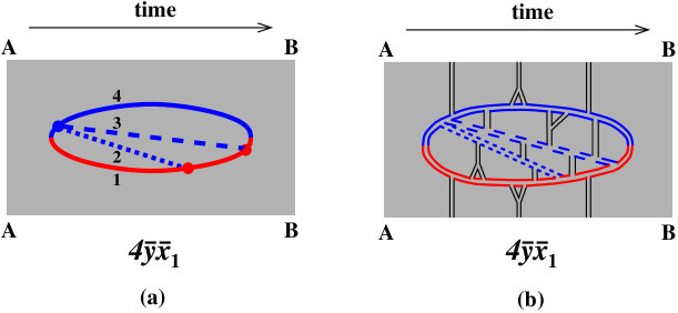
Figure 11: One of the two distinct large-$N_{\rm c}$ color routings of the $4\bar{y}\bar{x}$ interference diagram drawn on a cylinder (similar to fig. 23 of ref. seq , and following the general convention of refs. 2brem ; seq for discussing time-ordered large-$N_{\rm c}$ planar diagrams). The top edge AB of the shaded region is to be identified with the bottom edge AB. (b) explicitly shows the corresponding color flow for an example of medium background field correlations (black) that gives a planar diagram (and so leading-order in $1/N_{\rm c}$). In our notation, this interference contribution could be referred to as either $4\bar{y}\bar{x}_{1}$ or $4\bar{y}\bar{z}_{2}$.

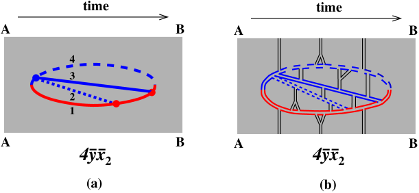
Figure 12: As fig. 11 but showing the other distinct color routing of $4\bar{y}\bar{x}$. In our notation, this interference contribution could be referred to as either $4\bar{y}\bar{x}_{2}$ or $4\bar{y}\bar{z}_{1}$.

Like the situation for the $xy\bar{x}\bar{y}$ diagram discussed in ref. seq , the distinguishing difference between the calculation of the two color routings is the assignment of the longitudinal momentum fractions $x_{i}$ for the 4-particle part of the evolution, which occurs here for $t_{(4)}<t<t_{\bar{\rm y}}$. Going around the cylinder depicted in fig. 11, the first routing $4\bar{y}\bar{x}_{1}$ has

$$(x_{1},x_{2},x_{3},x_{4})=(-1,y,x,1{-}x{-}y),$$ (7)

whereas the second routing $4\bar{y}\bar{x}_{2}$ of fig. 12 has

$$(x_{1},x_{2},x_{3},x_{4})=(-1,y,1{-}x{-}y,x)\equiv(\hat{x}_{1},\hat{x}_{2},\hat{x}_{3},\hat{x}_{4}).$$ (8)

Note that the ordering of the $x_{i}$ does not matter until we take the large-$N_{\rm c}$ limit and decide that the 4-particle propagator $\langle{\bm{C}}_{34}^{\bar{\rm y}},{\bm{C}}_{12}^{\bar{\rm y}},t_{\bar{\rm y}}|{\bm{C}}_{34}^{(4)},{\bm{C}}_{12}^{(4)},t_{(4)}\rangle$ will henceforth represent only a single color routing. That is why the $x_{i}$ assignment of fig. 8, before we discussed large-$N_{\rm c}$, could represent the entire contribution of $4\bar{y}\bar{x}$, but in our convention after we implement the large-$N_{\rm c}$ limit for discussion of the 4-particle propagator, the same assignment (8) now represents only a single color routing (fig. 12).

We will focus on the second routing (8) just because the assignment $x_{i}=\hat{x}_{i}$ is identical to the one used for the canonical diagram analyzed in ref. 2brem . We can obtain the other routing via $x\leftrightarrow z$:

$$\left[\frac{dI}{dx\,dy}\right]_{4\bar{y}\bar{x}}^{\rm total}=\left[\frac{dI}{dx\,dy}\right]_{4\bar{y}\bar{x}_{2}}+[x\leftrightarrow z].$$ (9)

The details of extracting what pieces of the color and helicity factors given by fig. 10 correspond to which of the two large-$N_{\rm c}$ color routings are a bit untidy. One can either (i) figure out how to split up the factors in fig. 10 or else (ii) switch to large-$N_{\rm c}$ Feynman rules. Here we’ll take the first option, as we found it the least confusing way to keep track of overall normalization factors.

If we label the gluon lines as $({\rm i},{\rm x},{\rm y},{\rm z})$ for the initial, $x$, $y$, and $z$ bosons, then the color and helicity factors given by fig. 10 for the 4-point vertex are

$$f^{a_{\rm i}a_{\rm x}e} f^{a_{\rm y}a_{\rm z}e}(\delta_{h_{\rm i},h_{\rm y}}\delta_{h_{\rm z},-h_{\rm x}}-\delta_{h_{\rm i},h_{\rm z}}\delta_{h_{\rm x},-h_{\rm y}})$$

$$+f^{a_{\rm i}a_{\rm y}e}f^{a_{\rm x}a_{\rm z}e}(\delta_{h_{\rm i},h_{\rm x}}\delta_{h_{\rm y},-h_{\rm z}}-\delta_{h_{\rm i},h_{\rm z}}\delta_{h_{\rm x},-h_{\rm y}})$$

$$+f^{a_{\rm i}a_{\rm z}e}f^{a_{\rm x}a_{\rm y}e}(\delta_{h_{\rm i},h_{\rm x}}\delta_{h_{\rm y},-h_{\rm z}}-\delta_{h_{\rm i},h_{\rm y}}\delta_{h_{\rm z},-h_{\rm x}}).$$ (10)

The large-$N_{\rm c}$ routing $4\bar{y}\bar{x}_{2}$ of fig. 12 corresponds to the first term above plus half of the second term,

$$f^{a_{\rm i}a_{\rm x}e} f^{a_{\rm y}a_{\rm z}e}(\delta_{h_{\rm i},h_{\rm y}}\delta_{h_{\rm z},-h_{\rm x}}-\delta_{h_{\rm i},h_{\rm z}}\delta_{h_{\rm x},-h_{\rm y}})$$

$$+\tfrac{1}{2}f^{a_{\rm i}a_{\rm y}e}f^{a_{\rm x}a_{\rm z}e}(\delta_{h_{\rm i},h_{\rm x}}\delta_{h_{\rm y},-h_{\rm z}}-\delta_{h_{\rm i},h_{\rm z}}\delta_{h_{\rm x},-h_{\rm y}}),$$ (11)

while the rest of (10) corresponds to the routing of fig. 11. The advantage of the large-$N_{\rm c}$ limit is that it then allows us to do a naive color contraction of the vertices in fig. 11a and 12a for each routing. In fig. 12a, (11) is contracted with adjoint color factors

$$(T_{\rm A}^{a_{\rm y}})_{a_{\rm i}\bar{a}}(T_{\rm A}^{a_{\rm x}})_{\bar{a}a_{\rm z}}=-f^{a_{\rm y}a_{\rm i}\bar{a}}f^{a_{\rm x}\bar{a}a_{\rm z}}$$ (12)

associated with the two 3-point vertices and averaged over initial color $a_{\rm i}$, giving

$$-\tfrac{1}{2}C_{\rm A}^{2}(\delta_{h_{\rm i},h_{\rm x}}\delta_{h_{\rm y},-h_{\rm z}}+\delta_{h_{\rm i},h_{\rm y}}\delta_{h_{\rm z},-h_{\rm x}}-2\delta_{h_{\rm i},h_{\rm z}}\delta_{h_{\rm x},-h_{\rm y}})$$ (13)

overall.

Using the rules for 3-gluon vertices, the general expression (3) then becomes

$$\left[\frac{dI}{dx\,dy}\right]_{4\bar{y}\bar{x}_{2}} =-\left(\frac{E}{2\pi}\right)^{2}\int_{t_{(4)}<t_{\bar{\rm y}}<t_{\bar{\rm x}}}\sum_{h_{\rm x},h_{\rm y},h_{\rm z},\bar{h}}\int_{{\bm{B}}^{\bar{\rm y}}}$$

$$\times\tfrac{i}{2}C_{\rm A}^{2}g^{4}(\delta_{h_{\rm i},h_{\rm x}}\delta_{h_{\rm y},-h_{\rm z}}+\delta_{h_{\rm i},h_{\rm y}}\delta_{h_{\rm z},-h_{\rm x}}-2\delta_{h_{\rm i},h_{\rm z}}\delta_{h_{\rm x},-h_{\rm y}})$$

$$\times\tfrac{1}{2}E^{-3/2}\,{\bm{\mathcal{P}}}_{{-}h_{\rm z},\bar{h},{-}h_{\rm x}}({-}\hat{x}_{3},\hat{x}_{3}{+}\hat{x}_{4},{-}\hat{x}_{4})\cdot{\bm{\nabla}}_{{\bm{B}}^{\bar{\rm x}}}\langle{\bm{B}}^{\bar{\rm x}},t_{\bar{\rm x}}|{\bm{B}}^{\bar{\rm y}},t_{\bar{\rm y}}\rangle\Bigr{|}_{{\bm{B}}^{\bar{\rm x}}=0}$$

$$\times\tfrac{1}{2}E^{-3/2}|\hat{x}_{3}+\hat{x}_{4}|^{-1}\,{\bm{\mathcal{P}}}_{{-}\bar{h},h_{\rm i},{-}h_{\rm y}}(\hat{x}_{1}{+}\hat{x}_{2},{-}\hat{x}_{1},{-}\hat{x}_{2})\cdot{\bm{\nabla}}_{{\bm{C}}_{12}^{\bar{\rm y}}}$$

$$\qquad\qquad\langle{\bm{C}}_{34}^{\bar{\rm y}},{\bm{C}}_{12}^{\bar{\rm y}},t_{\bar{\rm y}}|{\bm{C}}_{34}^{(4)},{\bm{C}}_{12}^{(4)},t_{(4)}\rangle\Bigr{|}_{{\bm{C}}_{12}^{\bar{\rm y}}=0={\bm{C}}_{34}^{(4)}={\bm{C}}_{12}^{(4)};~{}{\bm{C}}_{34}^{\bar{\rm y}}={\bm{B}}^{\bar{\rm y}}}$$

$$\times(2E)^{-2}|\hat{x}_{1}\hat{x}_{2}\hat{x}_{3}\hat{x}_{4}|^{-1/2}|\hat{x}_{3}+\hat{x}_{4}|^{-1}.$$ (14)

for the routing $4\bar{y}\bar{x}_{2}$. (See appendix A for details on the overall sign.)

II.3 Helicity Sums

For the helicity sums, we need

$$\sum_{h_{\rm x},h_{\rm y},h_{\rm z},\bar{h}}{\cal P}^{\bar{n}}_{{-}h_{\rm z},\bar{h},{-}h_{\rm x}}\bigl{(}{-}(1{-}x{-}y),1{-}y,{-}x\bigr{)}\,{\cal P}^{\bar{m}}_{{-}\bar{h},h_{\rm i},{-}h_{\rm y}}\bigl{(}{-}(1{-}y),1,{-}y\bigr{)}\\ \times(\delta_{h_{\rm i},h_{\rm x}}\delta_{h_{\rm y},-h_{\rm z}}+\delta_{h_{\rm i},h_{\rm y}}\delta_{h_{\rm z},-h_{\rm x}}-2\delta_{h_{\rm i},h_{\rm z}}\delta_{h_{\rm x},-h_{\rm y}})|\hat{x}_{1}\hat{x}_{2}\hat{x}_{3}\hat{x}_{4}|^{-1/2}$$ (15)

which is equivalent to

$$\sum_{h_{\rm x},h_{\rm y},h_{\rm z}}\Bigl{[}\sum_{\bar{h}}{\cal P}^{\bar{n}}_{\bar{h}\to h_{\rm z},h_{\rm x}}\bigl{(}1{-}y\to 1{-}x{-}y,x\bigr{)}\,{\cal P}^{\bar{m}}_{h_{\rm i}\to\bar{h},h_{\rm y}}\bigl{(}1\to 1{-}y,y\bigr{)}\Bigr{]}^{*}\\ \times(\delta_{h_{\rm i},h_{\rm x}}\delta_{h_{\rm y},-h_{\rm z}}+\delta_{h_{\rm i},h_{\rm y}}\delta_{h_{\rm z},-h_{\rm x}}-2\delta_{h_{\rm i},h_{\rm z}}\delta_{h_{\rm x},-h_{\rm y}})|\hat{x}_{1}\hat{x}_{2}\hat{x}_{3}\hat{x}_{4}|^{-1/2}.$$ (16)

Note that we have found it convenient to include the $|\hat{x}_{1}\hat{x}_{2}\hat{x}_{3}\hat{x}_{4}|^{-1/2}$ factor from (14) here.

By transverse parity invariance, we may average over the initial helicity. By transverse rotational invariance, the initial helicity average of (16) must be of the form

$$\zeta(x,y)\,\delta^{\bar{n}\bar{m}}$$ (17)

for some function $\zeta(x,y)$. Taking the formulas for the splitting functions ${\cal P}$ from ref. 2brem , we find

$$\zeta=\frac{2x^{2}-z^{2}-(1{-}y)^{4}+2y^{2}z^{2}-x^{2}y^{2}}{x^{2}y^{2}z^{2}(1{-}y)^{3}},$$ (18)

where $z\equiv 1{-}x{-}y$. Replacing (15) by (17) in (14) gives

$$\left[\frac{dI}{dx\,dy}\right]_{4\bar{y}\bar{x}_{2}}=-i\,\frac{C_{\rm A}^{2}\alpha_{\rm s}^{2}}{8E^{3}}\,\frac{\zeta}{|\hat{x}_{3}+\hat{x}_{4}|^{2}}\int_{t_{(4)}<t_{\bar{\rm y}}<t_{\bar{\rm x}}}\int_{{\bm{B}}^{\bar{\rm y}}}{\bm{\nabla}}_{{\bm{B}}^{\bar{\rm x}}}\langle{\bm{B}}^{\bar{\rm x}},t_{\bar{\rm x}}|{\bm{B}}^{\bar{\rm y}},t_{\bar{\rm y}}\rangle\Bigr{|}_{{\bm{B}}^{\bar{\rm x}}=0}\\ \cdot{\bm{\nabla}}_{{\bm{C}}_{12}^{\bar{\rm y}}}\langle{\bm{C}}_{34}^{\bar{\rm y}},{\bm{C}}_{12}^{\bar{\rm y}},t_{\bar{\rm y}}|{\bm{C}}_{34}^{(4)},{\bm{C}}_{12}^{(4)},t_{(4)}\rangle\Bigr{|}_{{\bm{C}}_{12}^{\bar{\rm y}}=0={\bm{C}}_{34}^{(4)}={\bm{C}}_{12}^{(4)};~{}{\bm{C}}_{34}^{\bar{\rm y}}={\bm{B}}^{\bar{\rm y}}}.$$ (19)

II.4 Harmonic Oscillator Approximation

Now take the harmonic oscillator approximation. As reviewed in ref. 2brem , for 3-particle evolution this corresponds to treating $\langle{\bm{B}},t|{\bm{B}}^{\prime},t^{\prime}\rangle$ as evolution of a two-dimensional harmonic oscillator with a certain effective mass $M$ and complex natural frequency $\Omega$. In the case of the final 3-particle evolution $t_{\bar{\rm y}}<t<t_{\bar{\rm x}}$ in figs. 8 and 12, these are 2brem

$$M_{\rm f}=\hat{x}_{3}\hat{x}_{4}(\hat{x}_{3}{+}\hat{x}_{4})E=x(1{-}y)(1{-}x{-}y)E$$ (20a)

and

$$\Omega_{\rm f}=\sqrt{-\frac{i\hat{q}_{\rm A}}{2E}\left(-\frac{1}{\hat{x}_{3}+\hat{x}_{4}}+\frac{1}{\hat{x}_{4}}+\frac{1}{\hat{x}_{3}}\right)}=\sqrt{-\frac{i\hat{q}_{\rm A}}{2E}\left(-\frac{1}{1{-}y}+\frac{1}{x}+\frac{1}{1{-}x{-}y}\right)}.$$ (20b)

Using a harmonic oscillator propagator gives

$$\int_{t_{\bar{\rm y}}}^{+\infty}dt_{\bar{\rm x}}\>{\bm{\nabla}}_{{\bm{B}}^{\bar{\rm x}}}\langle{\bm{B}}^{\bar{\rm x}},t_{\bar{\rm x}}|{\bm{B}}^{\bar{\rm y}},t_{\bar{\rm y}}\rangle\biggr{|}_{{\bm{B}}^{\bar{\rm x}}=0}=-\frac{iM_{\rm f}{\bm{B}}^{\bar{\rm y}}}{\pi(B^{\bar{\rm y}})^{2}}\,\exp\bigl{(}-\tfrac{1}{2}|M_{\rm f}|\Omega_{\rm f}(B^{\bar{\rm y}})^{2}\bigr{)},$$ (21)

which recasts (19) as

$$\left[\frac{d\Gamma}{dx\,dy}\right]_{4\bar{y}\bar{x}_{2}}=-\frac{C_{\rm A}^{2}\alpha_{\rm s}^{2}M_{\rm f}}{8\pi E^{3}}\,\frac{\zeta}{|\hat{x}_{3}+\hat{x}_{4}|^{2}}\int_{0}^{\infty}d(\Delta t)\int_{{\bm{B}}^{\bar{\rm y}}}\exp\bigl{(}-\tfrac{1}{2}|M_{\rm f}|\Omega_{\rm f}(B^{\bar{\rm y}})^{2}\bigr{)}\\ \times\frac{{\bm{B}}^{\bar{\rm y}}}{(B^{\bar{\rm y}})^{2}}\cdot{\bm{\nabla}}_{{\bm{C}}_{12}^{\bar{\rm y}}}\langle{\bm{C}}_{34}^{\bar{\rm y}},{\bm{C}}_{12}^{\bar{\rm y}},\Delta t|{\bm{C}}_{34}^{(4)},{\bm{C}}_{12}^{(4)},0\rangle\Bigr{|}_{{\bm{C}}_{12}^{\bar{\rm y}}=0={\bm{C}}_{34}^{(4)}={\bm{C}}_{12}^{(4)};~{}{\bm{C}}_{34}^{\bar{\rm y}}={\bm{B}}^{\bar{\rm y}}},$$ (22)

where $\Delta t\equiv t_{\bar{\rm y}}-t_{(4)}$. We now treat the 4-particle propagator $\langle{\bm{C}}_{34}^{\bar{\rm y}},{\bm{C}}_{12}^{\bar{\rm y}},\Delta t|{\bm{C}}_{34}^{(4)},{\bm{C}}_{12}^{(4)},0\rangle$ just as in section V.C of ref. 2brem , except that here we have chosen to use the same basis $({\bm{C}}_{34},{\bm{C}}_{12})$ in both the bra and the ket. The propagator is given by

$$\exp\bigl{(}-\tfrac{1}{2}|M_{\rm f}| \Omega_{\rm f}(C_{34}^{\bar{\rm y}})^{2}\bigr{)}\,\langle{\bm{C}}_{34}^{\bar{\rm y}},{\bm{C}}_{12}^{\bar{\rm y}},\Delta t|{\bm{C}}_{34}^{(4)},{\bm{C}}_{12}^{(4)},0\rangle=$$

$$(2\pi i)^{-2}({-}x_{1}x_{2}x_{3}x_{4})|x_{3}{+}x_{4}|^{2}E^{2}\Omega_{+}\Omega_{-}\csc(\Omega_{+}\Delta t)\csc(\Omega_{-}\Delta t)$$

$$\times\exp\Biggl{[}-\frac{1}{2}\begin{pmatrix}{\bm{C}}^{(4)}_{34}\\ {\bm{C}}^{(4)}_{12}\end{pmatrix}^{\top}\!\begin{pmatrix}X_{(4)}&Y_{(4)}\\ Y_{(4)}&Z_{(4)}\end{pmatrix}\begin{pmatrix}{\bm{C}}^{(4)}_{34}\\ {\bm{C}}^{(4)}_{12}\end{pmatrix}-\frac{1}{2}\begin{pmatrix}{\bm{C}}^{\bar{\rm y}}_{34}\\ {\bm{C}}^{\bar{\rm y}}_{12}\end{pmatrix}^{\top}\!\begin{pmatrix}X_{\bar{\rm y}}&Y_{\bar{\rm y}}\\ Y_{\bar{\rm y}}&Z_{\bar{\rm y}}\end{pmatrix}\begin{pmatrix}{\bm{C}}^{\bar{\rm y}}_{34}\\ {\bm{C}}^{\bar{\rm y}}_{12}\end{pmatrix}$$

$$\qquad+\begin{pmatrix}{\bm{C}}^{(4)}_{34}\\ {\bm{C}}^{(4)}_{12}\end{pmatrix}^{\top}\!\begin{pmatrix}X_{{(4)}{\bar{\rm y}}}&Y_{{(4)}{\bar{\rm y}}}\\ \overline{Y}_{{(4)}{\bar{\rm y}}}&Z_{{(4)}{\bar{\rm y}}}\end{pmatrix}\begin{pmatrix}{\bm{C}}^{\bar{\rm y}}_{34}\\ {\bm{C}}^{\bar{\rm y}}_{12}\end{pmatrix}\Biggr{]},$$ (23)

where we have included on the left-hand side of (23) the additional factor $\exp\bigl{(}-\tfrac{1}{2}|M_{\rm f}|\Omega_{\rm f}(B^{\bar{\rm y}})^{2}\bigr{)}=\exp\bigl{(}-\tfrac{1}{2}|M_{\rm f}|\Omega_{\rm f}(C_{34}^{\bar{\rm y}})^{2}\bigr{)}$ from (22) because that makes the definitions of the symbols $X$, $Y$, and $Z$ more convenient for later use. Those symbols are then given by

$$\begin{pmatrix}X_{(4)}&Y_{(4)}\\ Y_{(4)}&Z_{(4)}\end{pmatrix} \equiv-ia_{(4)}^{-1\top}\underline{\Omega}\cot(\underline{\Omega}\,\Delta t)\,a_{(4)}^{-1},$$ (24a)

$$\begin{pmatrix}X_{\bar{\rm y}}&Y_{\bar{\rm y}}\\ Y_{\bar{\rm y}}&Z_{\bar{\rm y}}\end{pmatrix} \equiv\begin{pmatrix}|M_{\rm f}|\Omega_{\rm f}&0\\ 0&0\end{pmatrix}-ia_{\bar{\rm y}}^{-1\top}\underline{\Omega}\cot(\underline{\Omega}\,\Delta t)\,a_{\bar{\rm y}}^{-1},$$ (24b)

$$\begin{pmatrix}X_{{(4)}{\bar{\rm y}}}&Y_{{(4)}{\bar{\rm y}}}\\ \overline{Y}_{{(4)}{\bar{\rm y}}}&Z_{{(4)}{\bar{\rm y}}}\end{pmatrix} \equiv-ia_{(4)}^{-1\top}\underline{\Omega}\csc(\underline{\Omega}\,\Delta t)\,a_{\bar{\rm y}}^{-1},$$ (24c)

where (given our choice of basis at the 4-point vertex)

$$a_{(4)}=a_{\bar{\rm y}}=\begin{pmatrix}C^{+}_{34}&C^{-}_{34}\\ C^{+}_{12}&C^{-}_{12}\end{pmatrix}.$$ (25)

Above, $\underline{\Omega}\equiv\bigl{(}\begin{smallmatrix}\Omega_{+}&\\ &\Omega_{-}\end{smallmatrix}\bigr{)}$. Formulas from 2brem for the two 4-particle evolution frequencies $\Omega_{\pm}$ and the corresponding normal modes $(C_{34}^{\pm},C_{12}^{\pm})$ are collected in Appendix D.2.

Using (23) in (22) gives

$$\left[\frac{d\Gamma}{dx\,dy}\right]_{4\bar{y}\bar{x}_{2}}=\frac{C_{\rm A}^{2}\alpha_{\rm s}^{2}M_{\rm f}}{8\pi E^{3}}\,\frac{\zeta}{|\hat{x}_{3}+\hat{x}_{4}|^{2}}\int_{0}^{\infty}d(\Delta t)\int_{{\bm{B}}^{\bar{\rm y}}}(2\pi i)^{-2}(-\hat{x}_{1}\hat{x}_{2}\hat{x}_{3}\hat{x}_{4})|\hat{x}_{3}+\hat{x}_{4}|^{2}E^{2}\\ \times\Omega_{+}\Omega_{-}\csc(\Omega_{+}\,\Delta t)\csc(\Omega_{-}\,\Delta t)Y_{\bar{\rm y}}\exp\bigl{(}-\tfrac{1}{2}X_{\bar{\rm y}}(B^{\bar{\rm y}})^{2}\bigr{)}.$$ (26)

The Gaussian ${\bm{B}}^{\bar{\rm y}}$ integral is straightforward, yielding

$$\left[\frac{d\Gamma}{dx\,dy}\right]_{4\bar{y}\bar{x}_{2}}=-\frac{C_{\rm A}^{2}\alpha_{\rm s}^{2}M_{\rm f}}{16\pi^{2}E}\,(-\hat{x}_{1}\hat{x}_{2}\hat{x}_{3}\hat{x}_{4})\zeta\int_{0}^{\infty}d(\Delta t)\>\Omega_{+}\Omega_{-}\csc(\Omega_{+}\,\Delta t)\csc(\Omega_{-}\,\Delta t)\frac{Y_{\bar{\rm y}}}{X_{\bar{\rm y}}}\,.$$ (27)

Our final result for the $4\bar{y}\bar{x}$ diagram is the above formula together with the corresponding version of (9),

$$\left[\frac{d\Gamma}{dx\,dy}\right]_{4\bar{y}\bar{x}}^{\rm total}=\left[\frac{d\Gamma}{dx\,dy}\right]_{4\bar{y}\bar{x}_{2}}+[x\leftrightarrow z].$$ (28)

III The Other Diagrams

III.1 The $\bar{y}\bar{x}4$ diagram

The $\bar{y}\bar{x}4$ diagram is the third diagram of fig. 3. Instead of going through an explicit calculation, we can relate the answer for this diagram to the $4\bar{y}\bar{x}$ diagram computed in the last section, along the lines of how the $x\bar{y}y\bar{x}$ and $xy\bar{y}\bar{x}$ diagrams of fig. 1 were related in ref. 2brem .

The first thing to note is that all three diagrams shown explicitly in fig. 3 have the same factors of helicity contractions and DGLAP splitting functions associated with their vertices—these factors are unaffected by the time ordering of the 4-point vertex in the amplitude relative to the two vertices in the conjugate amplitude. As to the rest of the computation, note that the diagrams $\bar{y}\bar{x}4$ and $4\bar{x}\bar{y}$ in fig. 3 look like mirror images of each other except for the identification of which gluon has which momentum fraction. For each color routing, we show one way of making this change of identification in fig. 13. There, when reflecting $4\bar{y}\bar{x}$ into $\bar{y}\bar{x}4$, we change

$$(x_{1},x_{2},x_{3},x_{4})=(-1,y,x,1{-}x{-}y)$$ (29)

to

$$(x_{1},x_{2},x_{3},x_{4})=\bigl{(}-(1{-}x{-}y),-x,-y,1\bigr{)}$$ (30)

for the first color routing, and

$$(x_{1},x_{2},x_{3},x_{4})=(-1,y,1{-}x{-}y,x)$$ (31)

to

$$(x_{1},x_{2},x_{3},x_{4})=\bigl{(}-x,-(1{-}x{-}y),-y,1\bigr{)}$$ (32)

for the second. Both cases can be summarized as

$$(x_{1},x_{2},x_{3},x_{4})\to(-x_{4},-x_{3},-x_{2},-x_{1}).$$ (33)

We also need to appropriately change the mass $M$ used for the 3-particle part of the evolution. As for similar diagram transformations in ref. 2brem , this will be taken care of automatically if we write this mass in terms of the 4-particle $x_{i}$ as in (20a):

$$M=x_{3}x_{4}(x_{3}{+}x_{4})E,$$ (34)

which, for example, gives $M=x(1{-}y)(1{-}x{-}y)E$ (20a) for 3-particle evolution in the $4\bar{y}\bar{x}_{2}$ case of $(x_{1},x_{2},x_{3},x_{4})=(\hat{x}_{1},\hat{x}_{2},\hat{x}_{3},\hat{x}_{4})$ and gives $M=-y(1{-}y)E$ for the corresponding $\bar{y}\bar{x}4_{2}$ case $(x_{1},x_{2},x_{3},x_{4})=(-\hat{x}_{4},-\hat{x}_{3},-\hat{x}_{2},-\hat{x}_{1})$.

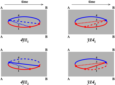
Figure 13: The two color routings of $4\bar{y}\bar{x}$ (left) compared to those of $\bar{y}\bar{x}4$ (right). There are many topologically-equivalent ways to draw the same diagram: we’ve chosen to draw the $\bar{y}\bar{x}4$ diagrams above in a way that gives a straightforward pictorial correspondence to our rule (33) for going from the $4\bar{y}\bar{x}$ diagrams on the left to the $\bar{y}\bar{x}4$ diagrams on the right.

The upshot is that we can convert the result for $4\bar{y}\bar{x}$ into a result for $\bar{y}\bar{x}4$ by (i) making the change (33) to the 4-particle $x_{i}$, (ii) always using the form (34) for the 3-particle evolution mass, and (iii) leaving $\zeta(x,y)$ unchanged. For the sake of readers wary of the glibness of the above argument, we give a more straightforward derivation of $\bar{y}\bar{x}4_{2}$ in appendix C and verify that the result is the same.

III.2 The $\bar{y}4\bar{x}$ diagram

Now consider the $\bar{y}4\bar{x}$ interference contribution, depicted by the second diagram in fig. 3. The starting point, analogous to (3), is

$$\left[\frac{dI}{dx\,dy}\right]_{\bar{y}4\bar{x}}=\left(\frac{E}{2\pi}\right)^{2}\int_{t_{\bar{\rm y}}<t_{(4)}<t_{\bar{\rm x}}}\sum_{\rm pol.}\langle|i\,\overline{\delta H}|{\bm{B}}^{\bar{\rm x}}\rangle\,\langle{\bm{B}}^{\bar{\rm x}},t_{\bar{\rm x}}|{\bm{B}}^{(4)},t_{(4)}\rangle\\ \times\langle{\bm{B}}^{(4)}|i\,\overline{\delta H}|{\bm{B}}^{\prime}{}^{(4)}\rangle\,\langle{\bm{B}}^{\prime}{}^{(4)},t_{(4)}|{\bm{B}}^{\bar{\rm y}},t_{\bar{\rm y}}\rangle\langle{\bm{B}}^{\bar{\rm y}}|i\,\overline{\delta H}|\rangle.$$ (35)

We will not need to work out the explicit normalization of the 4-gluon vertex matrix element $\langle{\bm{B}}^{(4)}|i\,\overline{\delta H}|{\bm{B}}^{\prime}{}^{(4)}\rangle$ (though we give it in Appendix B) because we will find that (35) is zero. The important point is that the helicity factors and splitting factors ${\cal P}$ are the same as they were for $4\bar{y}\bar{x}$ in section II.3, and so, using fig. 9,

$$\left[\frac{dI}{dx\,dy}\right]_{\bar{y}4\bar{x}}\propto\zeta\delta^{\bar{m}\bar{n}}\int_{t_{\bar{\rm y}}<t_{(4)}<t_{\bar{\rm x}}}\sum_{\rm pol.}\nabla^{\bar{n}}_{{\bm{B}}^{\bar{\rm x}}}\langle{\bm{B}}^{\bar{\rm x}},t_{\bar{\rm x}}|{\bm{B}}^{(4)},t_{(4)}\rangle\Bigl{|}_{{\bm{B}}^{\bar{\rm x}}=0={\bm{B}}^{(4)}}\\ \times\nabla^{\bar{m}}_{{\bm{B}}^{\bar{\rm y}}}\langle{\bm{B}}^{\prime}{}^{(4)},t_{(4)}|{\bm{B}}^{\bar{\rm y}},t_{\bar{\rm y}}\rangle\Bigl{|}_{{\bm{B}}^{\bar{\rm y}}=0={\bm{B}}^{\prime}{}^{(4)}}.$$ (36)

The reason that ${\bm{B}}^{(4)}$ and ${\bm{B}}^{\prime}{}^{(4)}$ are set to zero above is because in 3-particle evolution (analogous to the earlier statement about 4-particle evolution), the transverse positions ${\bm{b}}_{i}$ in our problem are implicitly constrained by the condition $x_{1}{\bm{b}}_{1}+x_{2}{\bm{b}}_{2}+x_{3}{\bm{b}}_{3}=0$ with $x_{1}+x_{2}+x_{3}=0$. (See section III of ref. 2brem .) One may use this constraint to show that there is but one relevant transverse degree of freedom for the three transverse positions in 3-particle evolution:

$${\bm{B}}\equiv\frac{{\bm{b}}_{1}-{\bm{b}}_{2}}{(x_{1}+x_{2})}=\frac{{\bm{b}}_{2}-{\bm{b}}_{3}}{(x_{2}+x_{3})}=\frac{{\bm{b}}_{3}-{\bm{b}}_{1}}{(x_{3}+x_{1})}\,.$$ (37)

So, in our application, when any two of the three particles are coincident, then ${\bm{B}}=0$ and all three of the particles are necessarily coincident.

But now we can see the result. The factors

$$\nabla^{\bar{n}}_{{\bm{B}}^{\bar{\rm x}}}\langle{\bm{B}}^{\bar{\rm x}},t_{\bar{\rm x}}|{\bm{B}}^{(4)},t_{(4)}\rangle\Bigl{|}_{{\bm{B}}^{\bar{\rm x}}=0={\bm{B}}^{(4)}}\qquad\mbox{and}\qquad\nabla^{\bar{m}}_{{\bm{B}}^{\bar{\rm y}}}\langle{\bm{B}}^{\prime}{}^{(4)},t_{(4)}|{\bm{B}}^{\bar{\rm y}},t_{\bar{\rm y}}\rangle\Bigl{|}_{{\bm{B}}^{\bar{\rm y}}=0={\bm{B}}^{\prime}{}^{(4)}}$$ (38)

must both be zero by parity, and so the $\bar{y}4\bar{x}$ contribution (36) vanishes.

III.3 The $4\bar{4}$ diagram

The $4\bar{4}$ diagram, shown in fig. 4, is formally given by

$$\left[\frac{dI}{dx\,dy}\right]_{4\bar{4}}=\left(\frac{E}{2\pi}\right)^{2}\int_{t_{(4)}<t_{(\bar{4})}}\sum_{\rm pol.}\langle|i\,\overline{\delta H}|{\bm{C}}_{34}^{(\bar{4})},{\bm{C}}_{12}^{(\bar{4})}\rangle\,\langle{\bm{C}}_{34}^{(\bar{4})},{\bm{C}}_{12}^{(\bar{4})},t_{(\bar{4})}|{\bm{C}}_{34}^{(4)},{\bm{C}}_{12}^{(4)},t_{(4)}\rangle\\ \times\langle{\bm{C}}_{34}^{(4)},{\bm{C}}_{12}^{(4)}|{-}i\,\delta H|\rangle.$$ (39)

This diagram has three distinct large-$N_{\rm c}$ color routings, shown in fig. 14, which are related by permutations of the three final-state gluons $(x,y,1{-}x{-}y)$.

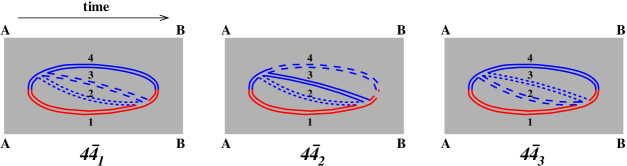
Figure 14: The three distinct large-$N_{\rm c}$ color routings of the $4\bar{4}$ interference diagram, drawn on a cylinder in large-$N_{\rm c}$ double-line notation. Other possible ways to draw color routings are equivalent. As usual, long-dashed and short-dashed lines refer to the gluons with momentum fraction $x$ and $y$ respectively.

The helicity and color factors associated with the 4-gluon matrix elements do not depend on the longitudinal momentum fractions (e.g. $x$ and $y$) of the various gluons and so, when summed over polarizations and colors, give the exact same helicity/color factor for each of the three color routings of fig. 14. Each is therefore a third of the total helicity/color factor $S$ we would get in a vacuum calculation, where we would not need to split the calculation into different color routings but could simply square and initial-state average the color/helicity factors (10) of the 4-point vertex:

$$S \equiv\frac{1}{2d_{\rm A}}\sum_{\mbox{\tiny$h$'s}}\sum_{\rm color}\Bigl{[}f^{a_{\rm i}a_{\rm x}e}f^{a_{\rm y}a_{\rm z}e}(\delta_{h_{\rm i},h_{\rm y}}\delta_{h_{\rm z},-h_{\rm x}}-\delta_{h_{\rm i},h_{\rm z}}\delta_{h_{\rm x},-h_{\rm y}})$$

$$\qquad\qquad\qquad+f^{a_{\rm i}a_{\rm y}e}f^{a_{\rm x}a_{\rm z}e}(\delta_{h_{\rm i},h_{\rm x}}\delta_{h_{\rm y},-h_{\rm z}}-\delta_{h_{\rm i},h_{\rm z}}\delta_{h_{\rm x},-h_{\rm y}})$$

$$\qquad\qquad\qquad+f^{a_{\rm i}a_{\rm z}e}f^{a_{\rm x}a_{\rm y}e}(\delta_{h_{\rm i},h_{\rm x}}\delta_{h_{\rm y},-h_{\rm z}}-\delta_{h_{\rm i},h_{\rm y}}\delta_{h_{\rm z},-h_{\rm x}})\Bigr{]}^{2}$$

$$=9C_{\rm A}^{2}$$ (40)

(where $d_{\rm A}$ is the dimension of the adjoint representation). So each color routing has a corresponding factor of $S/3=3C_{\rm A}^{2}$.

We will focus on the second color routing $4\bar{4}_{2}$, which is convenient because it again corresponds to our canonical choice (8),

$$(x_{1},x_{2},x_{3},x_{4})=(-1,y,1{-}x{-}y,x)\equiv(\hat{x}_{1},\hat{x}_{2},\hat{x}_{3},\hat{x}_{4}).$$ (41)

The corresponding contribution to (39) is

$$\left[\frac{dI}{dx\,dy}\right]_{4\bar{4}_{2}}=\left(\frac{E}{2\pi}\right)^{2}\int_{t_{(4)}<t_{(\bar{4})}}3C_{\rm A}^{2}g^{4}(2E)^{-4}|\hat{x}_{1}\hat{x}_{2}\hat{x}_{3}\hat{x}_{4}|^{-1}|\hat{x}_{3}+\hat{x}_{4}|^{-2}\\ \times\langle{\bm{C}}_{34}^{(\bar{4})},{\bm{C}}_{12}^{(\bar{4})},t_{(\bar{4})}|{\bm{C}}_{34}^{(4)},{\bm{C}}_{12}^{(4)},t_{(4)}\rangle\Bigr{|}_{{\rm all}~{}{\bm{C}}_{ij}=0}.$$ (42)

From (23),

$$\langle{\bm{C}}_{34}^{(\bar{4})},{\bm{C}}_{12}^{(\bar{4})},\Delta t|{\bm{C}}_{34}^{(4)},{\bm{C}}_{12}^{(4)},0\rangle\Bigr{|}_{{\rm all}~{}{\bm{C}}_{ij}=0}=\\ (2\pi i)^{-2}({-}x_{1}x_{2}x_{3}x_{4})|x_{3}{+}x_{4}|^{2}E^{2}\Omega_{+}\Omega_{-}\csc(\Omega_{+}\Delta t)\csc(\Omega_{-}\Delta t),$$ (43)

and so

$$\left[\frac{d\Gamma}{dx\,dy}\right]_{4\bar{4}_{2}}=-\frac{3C_{\rm A}^{2}\alpha_{\rm s}^{2}}{16\pi^{2}}\int_{0}^{\infty}d(\Delta t)\>\Omega_{+}\Omega_{-}\csc(\Omega_{+}\,\Delta t)\csc(\Omega_{-}\,\Delta t).$$ (44)

We may then sum all the color routings by adding appropriate permutations:

$$\left[\frac{d\Gamma}{dx\,dy}\right]_{4\bar{4}}^{\rm total}=\left[\frac{d\Gamma}{dx\,dy}\right]_{4\bar{4}_{2}}+[x\leftrightarrow z]+[y\leftrightarrow z].$$ (45)

Note that $\left[\frac{d\Gamma}{dx\,dy}\right]_{4\bar{4}}$ should be positive since it is the medium average of the magnitude-squared of something (the amplitude for double bremsstrahlung via the 4-gluon vertex in the background of the medium). The numerical result shown in fig. 7 verifies this is the case.

We also note in passing that we can evaluate (44) analytically in the limit that one of the final-state gluons in soft. For $y\ll x$ and $z$, the result for the total contribution of fig. 4 (i.e. adding in the conjugate diagrams) is

$$\left[\frac{d\Gamma}{dx\,dy}\right]_{(44)}\equiv 2\operatorname{Re}\left[\frac{d\Gamma}{dx\,dy}\right]_{4\bar{4}}\simeq 6\operatorname{Re}\left[\frac{d\Gamma}{dx\,dy}\right]_{4\bar{4}_{2}}\simeq\frac{9C_{\rm A}^{2}\alpha_{\rm s}^{2}\ln 2}{16\pi^{2}}\sqrt{\frac{\hat{q}_{\rm A}}{yE}}\qquad(y\ll x,z).$$ (46)

(See appendix A.)

IV Summary of Formula

The total result for the correction $\Delta\,d\Gamma/dx\,dy$ due to overlapping formation times is

$$\Delta\frac{d\Gamma}{dx\,dy}=\left[\frac{d\Gamma}{dx\,dy}\right]_{\rm crossed}+\left[\Delta\frac{d\Gamma}{dx\,dy}\right]_{\rm seq}+\left[\frac{d\Gamma}{dx\,dy}\right]_{(4)}+\left[\frac{d\Gamma}{dx\,dy}\right]_{(44)},$$ (47)

where $[d\Gamma/dx\,dy]_{\rm crossed}$ and $[\Delta\,d\Gamma/dx\,dy]_{\rm seq}$ are given respectively in ref. 2brem ; dimreg and ref. seq . For completeness, we have summarized those formulas in Appendix D. The contributions new to this paper, involving one or more 4-gluon vertices, are summarized below.

IV.1 Diagrams with one 4-gluon vertex

The diagrams of fig. 3 (including all permutations, large-$N_{\rm c}$ color routings, and conjugates) give the following contribution to $d\Gamma/dx\>dy$:

$$\left[\frac{d\Gamma}{dx\>dy}\right]_{(4)}=\quad {\cal A}_{(4)}(x,y)+{\cal A}_{(4)}(1{-}x{-}y,y)+{\cal A}_{(4)}(x,1{-}x{-}y)$$

$$+~{} {\cal A}_{(4)}(y,x)+{\cal A}_{(4)}(y,1{-}x{-}y)+{\cal A}_{(4)}(1{-}x{-}y,x)$$ (48)

where ${\cal A}_{(4)}(x,y)$ is the result for one color routing of $4\bar{y}\bar{x}+\bar{y}4\bar{x}+\bar{y}\bar{x}4$ plus conjugates. We will write this as

$${\cal A}_{(4)}(x,y)\equiv\int_{0}^{+\infty}d(\Delta t)\>2\operatorname{Re}\bigl{(}B_{(4)}(x,y,\Delta t)\bigr{)}$$ (49)

where

$$B_{(4)}(x,y,\Delta t) =D_{(4)}(\hat{x}_{1},\hat{x}_{2},\hat{x}_{3},\hat{x}_{4},\zeta,\Delta t)+D_{(4)}(-\hat{x}_{4},-\hat{x}_{3},-\hat{x}_{2},-\hat{x}_{1},\zeta,\Delta t)$$

$$=D_{(4)}({-}1,y,1{-}x{-}y,x,\zeta,\Delta t)+D_{(4)}(-x,-(1{-}x{-}y),-y,1,\zeta,\Delta t)$$ (50)

corresponds to (i) the $4\bar{y}\bar{x}_{2}$ color routing of $4\bar{y}\bar{x}$ plus (ii) the related color routing $\bar{y}\bar{x}4_{2}$ of $\bar{y}\bar{x}4$. $\zeta=\zeta(x,y)$ is given by (18). Each of the terms in (50) is given by

$$D_{(4)}(x_{1}, x_{2},x_{3},x_{4},\zeta,\Delta t)=$$

$$-\frac{C_{\rm A}^{2}\alpha_{\rm s}^{2}M_{\rm f}}{16\pi^{2}E}\,(-x_{1}x_{2}x_{3}x_{4})\zeta\Omega_{+}\Omega_{-}\csc(\Omega_{+}\,\Delta t)\csc(\Omega_{-}\,\Delta t)\frac{Y_{\bar{\rm y}}}{X_{\bar{\rm y}}}\,,$$ (51)

which is the integrand of (27). Here, the $X,Y,Z$ are defined by (24) and (25), with

$$M_{\rm f} =x_{3}x_{4}(x_{3}{+}x_{4})E,$$ (52)

$$\Omega_{\rm f} =\sqrt{-\frac{i\hat{q}_{\rm A}}{2E}\left(\frac{1}{x_{3}}+\frac{1}{x_{4}}-\frac{1}{x_{3}{+}x_{4}}\right)}.$$ (53)

As mentioned earlier, explicit formulas for the 4-particle evolution frequencies $\Omega_{\pm}$ in terms of $(x_{1},x_{2},x_{3},x_{4})$ are collected in Appendix D.2.

Unlike for the crossed and sequential diagrams analyzed in refs. 2brem ; seq , it is unnecessary to explicitly subtract the vacuum contribution from $D_{(4)}$. That’s because the vacuum limit $\hat{q}\to 0$ (and so $\Omega_{\pm}\to 0$ and $\Omega_{\rm f}\to 0$) of (51) already vanishes.

Also unlike the crossed and sequential diagrams 2brem ; seq , there are no $1/\Delta t$ divergences associated with the individual diagrams of fig. 3, and so there are no “pole” term contributions that need to be included in ${\cal A}_{(4)}$ above.

IV.2 Diagrams with two 4-gluon vertices

The diagrams of fig. 4 give the following contribution:

$$\left[\frac{d\Gamma}{dx\>dy}\right]_{(44)}={\cal A}_{(44)}(x,y)+{\cal A}_{(44)}(1{-}x{-}y,y)+{\cal A}_{(44)}(x,1{-}x{-}y)$$ (54)

where ${\cal A}_{(44)}(x,y)$ is the result for one color routing of $4\bar{4}$ plus conjugate. We write this as

$${\cal A}_{(44)}(x,y)\equiv\int_{0}^{+\infty}d(\Delta t)\>2\operatorname{Re}\bigl{(}B_{(44)}(x,y,\Delta t)\bigr{)}$$ (55)

where

$$B_{(44)}(x,y,\Delta t) =C_{(44)}(\hat{x}_{1},\hat{x}_{2},\hat{x}_{3},\hat{x}_{4},\Delta t)=C_{(44)}({-}1,y,1{-}x{-}y,x,\Delta t)$$ (56)

corresponds to the color routing $4\bar{4}_{2}$ with vacuum subtraction. The vacuum subtraction is

$$C_{(44)}=D_{(44)}-\lim_{\hat{q}\to 0}D_{(44)},$$ (57)

where $D_{(44)}$ is the unsubtracted result extracted from (44),

$$D_{(44)}(x_{1},x_{2},x_{3},x_{4},\Delta t)=-\frac{3C_{\rm A}^{2}\alpha_{\rm s}^{2}}{16\pi^{2}}\,\Omega_{+}\Omega_{-}\csc(\Omega_{+}\,\Delta t)\csc(\Omega_{-}\,\Delta t).$$ (58)

Again, there are no $1/\Delta t$ divergences associated with the diagrams here, and so there are no “pole” term contributions that need to be included in ${\cal A}_{(4\bar{4})}$ above.

V Conclusion

We have now completed the calculation of the overlapping formation time correction to double bremsstrahlung for the process $g\to ggg$ of emitting two real bremsstrahlung gluons from an initial gluon. The size of interference terms involving 4-gluon vertices had to be computed (i) for completeness and (ii) to see how big they are. However, the conclusion we can take from the numerical results of figs. 5–7 is that their effect on the result is small and one would not go far wrong in ignoring them, at least insofar as $\Delta\,d\Gamma/dx\,dy$ is concerned.

An important reason for calculating the overlapping formation time correction is to test whether it is large or small for realistic value of $\alpha_{\rm s}$. It is already known that the corrections due to soft bremsstrahlung ($y\ll 1$) are large due to large logarithms but that such soft corrections can be resummed into a running value of $\hat{q}$ that depends on energy Wu0 ; Blaizot1 ; Blaizot ; Iancu ; Wu ; Iancu2 . But what about the contribution from overlapping hard bremsstrahlung, which cannot be absorbed into $\hat{q}$? In the thick-medium approximation used here, these corrections are controlled by the value of $\alpha_{\rm s}$ at scales of order $Q_{\perp}\sim(\hat{q}E)^{1/4}$. An answer concerning the size of these non-absorbable corrections will need to wait longer until we are in a position to calculate an infrared-safe physical quantity characterizing shower development, which will require (i) including the effects of virtual corrections to single bremsstrahlung and (ii) consistent factorization of the effects of soft bremsstrahlung into $\hat{q}$.

Appendix A More details on some formulas

Eq. (14):

The overall sign of this formula arises as follows, similar to the discussion of AI (4.16) in Appendix A of ref. 2brem . Consider first the rule associated with the $t=t_{\bar{\rm y}}$ vertex in fig. 8 (remembering that the ordering of $x_{i}$ used in that figure was chosen to match the ordering of the large-$N_{\rm c}$ color routing $4\bar{y}\bar{x}_{2}$ of fig. 12). According to the rules of fig. 9, this vertex comes with a factor of $(T_{R}^{a_{k}})_{a_{j}a_{i}}{\bm{\nabla}}\delta^{(2)}({\bm{\mathcal{B}}}_{ji})$, with lines $(i,j,k)$ identified as in the figure. Using the cyclic permutation identity ${\bm{\mathcal{B}}}_{ji}={\bm{\mathcal{B}}}_{kj}={\bm{\mathcal{B}}}_{ik}$ noted in the caption, and comparing fig. 9 to the $t=t_{\bar{\rm y}}$ vertex in fig. 8, we can identify these factors as $(T_{R}^{a_{k}})_{a_{j}a_{i}}{\bm{\nabla}}\delta^{(2)}({\bm{\mathcal{B}}}_{kj})=(T_{\rm A}^{a_{\rm y}})_{a_{\rm i}\bar{a}}{\bm{\nabla}}\delta^{(2)}({\bm{C}}_{21})$. Similarly, the vertex at $t=t_{\bar{\rm x}}$ comes with a factor of $(T_{R}^{a_{k}})_{a_{j}a_{i}}{\bm{\nabla}}\delta^{(2)}({\bm{\mathcal{B}}}_{ik})=(T_{\rm A}^{a_{\rm x}})_{\bar{a}a_{\rm z}}{\bm{\nabla}}\delta^{(2)}({\bm{C}}_{34})$. Since we have identified ${\bm{C}}_{34}$ with ${\bm{B}}$ in (14), the latter is $(T_{\rm A}^{a_{\rm x}})_{\bar{a}a_{\rm z}}{\bm{\nabla}}\delta^{(2)}({\bm{B}})$. The color factors $(T_{\rm A}^{a_{\rm y}})_{a_{\rm i}\bar{a}}(T_{\rm A}^{a_{\rm x}})_{\bar{a}a_{\rm z}}$ from these two vertices (and the signs that arise from them) have already been accounted for in (12), which has already been combined with the 4-gluon vertex factor (and its signs) in (13). We are left with the $\delta$-function factors ${\bm{\nabla}}\delta^{(2)}({\bm{C}}_{21})\,{\bm{\nabla}}\delta^{(2)}({\bm{B}})$. Since ${\bm{C}}_{21}=-{\bm{C}}_{12}$, these may be rewritten as

$$-{\bm{\nabla}}\delta^{(2)}({\bm{C}}_{12})\,{\bm{\nabla}}\delta^{(2)}({\bm{B}}),$$ (59)

which is the form used in (14), where both ${\bm{C}}_{12}$ and ${\bm{B}}$ have been integrated by parts. This minus sign combines with the minus sign in (13) and the $\mp=-$ in fig. 10 to give the overall minus sign in (14).

Eq. (46):

In the limit that $y$ is small compared to both $x$ and $z\equiv 1{-}x{-}y$, the formulas for the 4-particle frequencies $\Omega_{\pm}$ collected in appendix D.2 satisfy, for the case $x_{i}=\hat{x}_{i}$,

$$\Omega_{-}\ll\Omega_{+}\simeq\Omega_{y}\equiv\sqrt{-\frac{i\hat{q}_{\rm A}}{2yE}}\,.$$ (60)

The factor of $\csc(\Omega_{+}\,\Delta t)$ in (44) means that the integrand is negligible unless $\Omega_{+}\Delta t\lesssim 1$, in which case $\Omega_{-}\Delta t\ll 1$. So the integral may be approximated as

$$\left[\frac{d\Gamma}{dx\,dy}\right]_{4\bar{4}_{2}}\simeq-\frac{3C_{\rm A}^{2}\alpha_{\rm s}^{2}}{16\pi^{2}}\int_{0}^{\infty}\frac{d(\Delta t)}{\Delta t}\>\Omega_{y}\csc(\Omega_{y}\,\Delta t).$$ (61)

This approximation is the same for all three color routings. Correspondingly multiplying by 3, and then adding in the conjugate diagram $\bar{4}4$ by taking twice the real part,

$$\left[\frac{d\Gamma}{dx\,dy}\right]_{(44)}\simeq-\frac{9C_{\rm A}^{2}\alpha_{\rm s}^{2}}{8\pi^{2}}\operatorname{Re}\int_{0}^{\infty}\frac{d(\Delta t)}{\Delta t}\>\Omega_{y}\csc(\Omega_{y}\,\Delta t).$$ (62)

As we do with all diagrams, we now subtract out the vacuum contribution $\hat{q}\to 0$ (i.e. $\Omega_{y}\to 0$), leaving

$$\left[\frac{d\Gamma}{dx\,dy}\right]_{(44)} \simeq-\frac{9C_{\rm A}^{2}\alpha_{\rm s}^{2}}{8\pi^{2}}\operatorname{Re}\int_{0}^{\infty}\frac{d(\Delta t)}{\Delta t}\left[\Omega_{y}\csc(\Omega_{y}\,\Delta t)-\frac{1}{\Delta t}\right]$$

$$=-\frac{9C_{\rm A}^{2}\alpha_{\rm s}^{2}}{8\pi^{2}}\operatorname{Re}\left(i\Omega_{y}\int_{0}^{\infty}\frac{d\tau}{\tau}\left[\frac{1}{\operatorname{sh}\tau}-\frac{1}{\tau}\right]\right)$$

$$=\frac{9C_{\rm A}^{2}\alpha_{\rm s}^{2}\ln 2}{8\pi^{2}}\operatorname{Re}(i\Omega_{y}),$$ (63)

which gives (46).

Appendix B The 4-gluon matrix element

B.1 $\langle{\bm{C}}_{34},{\bm{C}}_{12}|\delta H|\rangle$

To derive the matrix element $\langle{\bm{C}}_{34},{\bm{C}}_{12}|\delta H|\rangle$, we will follow the method used for deriving other matrix elements in Appendix B of ref. 2brem . We start in a description of states where we individually distinguish each high-energy particle, using the conventions of fig. 15a. First, the $\delta H$ matrix element in the amplitude, written conventionally in terms of the individual particles in the Hilbert space ${\mathbb{H}}$ (as opposed to the Hilbert space $\bar{\mathbb{H}}\otimes{\mathbb{H}}$ used to simultaneously describe particles in the amplitude and conjugate amplitude), is

$$\langle{\bm{b}}_{2},{\bm{b}}_{3},{\bm{b}}_{4}|\delta H|{\bm{b}}_{2}^{\prime}\rangle={\mathfrak{H}}\,\delta^{(2)}({\bm{b}}_{2}{-}{\bm{b}}_{2}^{\prime})\,\delta^{(2)}({\bm{b}}_{3}{-}{\bm{b}}_{2})\,\delta^{(2)}({\bm{b}}_{4}{-}{\bm{b}}_{2})$$ (64)

with

$${\mathfrak{H}}\equiv g^{2} \Bigl{[}f^{a_{1}a_{2}e}f^{a_{3}a_{4}e}(\delta_{h_{1},-h_{3}}\delta_{h_{4},-h_{2}}-\delta_{h_{1},-h_{4}}\delta_{h_{2},-h_{3}})$$

$$\quad+f^{a_{1}a_{3}e}f^{a_{2}a_{4}e}(\delta_{h_{1},-h_{2}}\delta_{h_{3},-h_{4}}-\delta_{h_{1},-h_{4}}\delta_{h_{2},-h_{3}})$$

$$\quad+f^{a_{1}a_{4}e}f^{a_{2}a_{3}e}(\delta_{h_{1},-h_{2}}\delta_{h_{3},-h_{4}}-\delta_{h_{1},-h_{3}}\delta_{h_{4},-h_{2}})\Bigr{]}$$

$$\times(2|x_{1}|E)^{-1/2}(2|x_{2}|E)^{-1/2}(2|x_{3}|E)^{-1/2}(2|x_{4}|E)^{-1/2}.$$ (65)

(64) is the usual relativistic formula except for a few small differences. The factors of $(2E_{i})^{-1/2}=(2|x_{i}|E)^{-1/2}$ for each particle above are included because we use non-relativistic rather than relativistic normalization for the states. We have written the rule in transverse ${\bm{b}}$-space instead of transverse momentum space, so there are $\delta$-functions requiring the points to be coincident at the vertex instead of a $\delta$-function for overall transverse momentum conservation. We have assumed that the longitudinal momenta have already been chosen to satisfy longitudinal momentum conservation, and we have (just as in ref. 2brem ) chosen a normalization of our states where we implicitly drop the corresponding momentum-space $\delta(p_{2z}^{\prime}{-}p_{2z}{-}p_{3z}{-}p_{4z})$. Finally, we have used the fact that the initial state represents a single on-shell particle to link the color and helicity of particle $2^{\prime}$ to that of $1^{\prime}$ and thus, via fig. 15a, to particle $1$. We have accordingly chosen to label the corresponding color and helicity indices in (65) by $1$ instead of by $2^{\prime}$. The convention used for the flow of helicity here is that of fig. 10. The $\delta_{\cdots}\delta_{\cdots}$ terms in (65) for helicity come from contracting the usual factors $g_{\mu\nu}g_{\alpha\beta}$ in the Feynman rule for the 4-point vertex with normalized helicity polarizations $\epsilon_{(h)}^{\mu}$ for each particle.

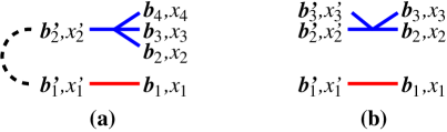
Figure 15: The notation used in (a) appendix B.1 and (b) appendix B.2 to label different particles’ states immediately before and after a 4-gluon vertex. The dashed connection in (a) indicates the fact that in this case the initial particles in the amplitude and conjugate amplitude represent the same particle (and so, for instance, ${\bm{b}}_{1}^{\prime}={\bm{b}}_{2}^{\prime}$ and, given our conventions, $x_{1}^{\prime}=-x_{2}^{\prime}$).

The corresponding matrix element in the space $\bar{\mathbb{H}}\otimes{\mathbb{H}}$ that includes the particle in the conjugate amplitude is

$$\langle{\bm{b}}_{1},{\bm{b}}_{2},{\bm{b}}_{3},{\bm{b}}_{4}|\delta H|{\bm{b}}_{1}^{\prime},{\bm{b}}_{2}^{\prime}\rangle=\langle{\bm{b}}_{2},{\bm{b}}_{3},{\bm{b}}_{4}|\delta H|{\bm{b}}_{2}^{\prime}\rangle\,\delta^{(2)}({\bm{b}}_{1}{-}{\bm{b}}_{1}^{\prime}).$$ (66)

Next we want to use the symmetry of the problem to project each state onto a subspace with two fewer degrees of freedom, as discussed in AI section III and AI Appendix B 2brem . Using the notation of that reference,

$$\langle\{{\bm{C}}_{ij}\}|\delta H|\rangle=\frac{1}{{\widetilde{V}}_{\perp}}\int_{\Delta{\bm{b}}}\langle{\bm{b}}_{1},{\bm{b}}_{2},{\bm{b}}_{3},{\bm{b}}_{4}|\delta H|{\bm{b}}_{1}^{\prime}{+}\Delta{\bm{b}},{\bm{b}}_{2}^{\prime}{+}\Delta{\bm{b}}\rangle,$$ (67)

where it is understood that both the initial and final positions satisfy the constraint $\sum_{i}x_{i}{\bm{b}}_{i}=0$ and where ${\widetilde{V}}_{\perp}$ is a formally infinite normalization given by

$${\widetilde{V}}_{\perp}\equiv\delta^{(2)}({\textstyle\sum}x_{i}{\bm{b}}_{i})\Bigr{|}_{\sum x_{i}{\bm{b}}_{i}=0}.$$ (68)

Using (64) and (66),

$$\langle\{{\bm{C}}_{ij}\}|\delta H|\rangle =\frac{\mathfrak{H}}{{\widetilde{V}}_{\perp}}\int_{\Delta{\bm{b}}}\delta^{(2)}({\bm{b}}_{1}-{\bm{b}}_{1}^{\prime}{-}\Delta{\bm{b}})\,\delta^{(2)}({\bm{b}}_{2}{-}{\bm{b}}_{2}^{\prime}{-}\Delta{\bm{b}})\,\delta^{(2)}({\bm{b}}_{3}{-}{\bm{b}}_{2})\,\delta^{(2)}({\bm{b}}_{4}{-}{\bm{b}}_{2})$$

$$=\frac{\mathfrak{H}}{{\widetilde{V}}_{\perp}}\,\delta^{(2)}({\bm{b}}_{12}{-}{\bm{b}}_{12}^{\prime})\,\delta^{(2)}({\bm{b}}_{32})\,\delta^{(2)}({\bm{b}}_{42}),$$ (69)

where ${\bm{b}}_{ij}\equiv{\bm{b}}_{i}-{\bm{b}}_{j}$. The initial state $|{\bm{b}}_{1}^{\prime},{\bm{b}}_{2}^{\prime}\rangle$ satisfies the constraint $x_{1}^{\prime}{\bm{b}}_{1}^{\prime}+x_{2}^{\prime}{\bm{b}}_{2}^{\prime}=0$ with $x_{1}^{\prime}+x_{2}^{\prime}=0$, and therefore ${\bm{b}}_{12}^{\prime}=0$, giving

$$\langle\{{\bm{C}}_{ij}\}|\delta H|\rangle=\frac{\mathfrak{H}}{{\widetilde{V}}_{\perp}}\,\delta^{(2)}({\bm{b}}_{12})\,\delta^{(2)}({\bm{b}}_{32})\,\delta^{(2)}({\bm{b}}_{42}).$$ (70)

Given the presence of the other two $\delta$-functions, the first one can be rewritten as

$$\delta^{(2)}({\bm{b}}_{12})=x_{1}^{2}\,\delta^{(2)}(x_{1}{\bm{b}}_{12}{+}x_{3}{\bm{b}}_{32}{+}x_{4}{\bm{b}}_{42})=x_{1}^{2}\,\delta^{(2)}(x_{1}{\bm{b}}_{1}{+}x_{2}{\bm{b}}_{2}{+}x_{3}{\bm{b}}_{3}{+}x_{4}{\bm{b}}_{4}),$$ (71)

where the last equality uses

$$x_{1}+x_{2}+x_{3}+x_{4}=0.$$ (72a)

Since

$$x_{1}{\bm{b}}_{1}+x_{2}{\bm{b}}_{2}+x_{3}{\bm{b}}_{3}+x_{4}{\bm{b}}_{4}=0$$ (72b)

as well, the substitution (71) in (70) gives

$$\langle\{{\bm{C}}_{ij}\}|\delta H|\rangle=\mathfrak{H}x_{1}^{2}\,\delta^{(2)}({\bm{b}}_{32})\,\delta^{(2)}({\bm{b}}_{42})$$ (73)

by (68). Because of the constraints (72), the variables ${\bm{b}}_{32}$ and ${\bm{b}}_{42}$ are related to ${\bm{C}}_{12}\equiv{\bm{b}}_{12}/(x_{1}{+}x_{2})$ and ${\bm{C}}_{34}\equiv{\bm{b}}_{34}/(x_{3}{+}x_{4})$ by

$${\bm{b}}_{32} =-{\bm{b}}_{23}=x_{1}{\bm{C}}_{12}+x_{4}{\bm{C}}_{34},$$ (74a)

$${\bm{b}}_{42} =-{\bm{b}}_{24}=x_{1}{\bm{C}}_{12}-x_{3}{\bm{C}}_{34},$$ (74b)

and the Jacobean for the change of variables is $\partial({\bm{b}}_{32},{\bm{b}}_{42})/\partial({\bm{C}}_{12},{\bm{C}}_{34})=[x_{1}(x_{3}{+}x_{4})]^{2}.$ So (73) can be rewritten as

$$\langle\{{\bm{C}}_{ij}\}|\delta H|\rangle=\frac{\mathfrak{H}}{(x_{3}{+}x_{4})^{2}}\,\delta^{(2)}({\bm{C}}_{12})\,\delta^{(2)}({\bm{C}}_{34}).$$ (75)

Changing normalization as in ref. 2brem ,

$$|{\bm{C}}_{34},{\bm{C}}_{12}\rangle\equiv|x_{3}{+}x_{4}|\,\bigl{|}\{{\bm{C}}_{ij}\}\bigr{\rangle},$$ (76)

then gives the matrix element (6) displayed in the main text.

B.2 $\langle{\bm{B}}|\delta H|{\bm{B}}^{\prime}\rangle$

We do not need to figure out the correct normalization of the matrix element $\langle{\bm{B}}|\delta H|{\bm{B}}^{\prime}\rangle$ for this paper, but we do so here just for the sake of completeness. The corresponding diagrammatic rule we will find is shown in fig. 16.

Figure 16: As fig. 10 but for the case with an an additional spectator (e.g. as in the $\bar{y}4\bar{x}$ diagram of fig. 3).

Analogous to (64), start with the amplitude matrix element

$$\langle{\bm{b}}_{2},{\bm{b}}_{3}|\delta H|{\bm{b}}_{2}^{\prime},{\bm{b}}_{3}^{\prime}\rangle={\mathfrak{H}}^{\prime}\,\delta^{(2)}({\bm{b}}_{2}{-}{\bm{b}}_{2}^{\prime})\,\delta^{(2)}({\bm{b}}_{3}{-}{\bm{b}}_{3}^{\prime})\,\delta^{(2)}({\bm{b}}_{3}{-}{\bm{b}}_{2}),$$ (77)

using the labeling of fig. 15b. Here ${\mathfrak{H}}^{\prime}$ is the same as (65) except that the indices $1$ and $4$ are replaced by $2^{\prime}$ and $3^{\prime}$. Including the particle in the conjugate amplitude,

$$\langle{\bm{b}}_{1},{\bm{b}}_{2},{\bm{b}}_{3}|\delta H|{\bm{b}}_{1}^{\prime},{\bm{b}}_{2}^{\prime},{\bm{b}}_{3}^{\prime}\rangle=\langle{\bm{b}}_{2},{\bm{b}}_{3}|\delta H|{\bm{b}}_{2}^{\prime},{\bm{b}}_{3}^{\prime}\rangle\,\delta^{(2)}({\bm{b}}_{1}{-}{\bm{b}}_{1}^{\prime}).$$ (78)

Projecting the number of degrees of freedom in each state from 3 to 1 as in ref. 2brem ,

$$\langle{\bm{B}}|\delta H|{\bm{B}}^{\prime}\rangle =\frac{1}{{\widetilde{V}}_{\perp}}\int_{\Delta{\bm{b}}}\langle{\bm{b}}_{1}{\bm{b}}_{2},{\bm{b}}_{3}|\delta H|{\bm{b}}_{1}^{\prime}{+}\Delta{\bm{b}},{\bm{b}}_{2}^{\prime}{+}\Delta{\bm{b}},{\bm{b}}_{3}^{\prime}{+}\Delta{\bm{b}}\rangle$$

$$=\frac{{\mathfrak{H}}^{\prime}}{{\widetilde{V}}_{\perp}}\,\delta^{(2)}({\bm{b}}_{21}{-}{\bm{b}}_{21}^{\prime})\,\delta^{(2)}({\bm{b}}_{31}{-}{\bm{b}}_{31}^{\prime})\,\delta^{(2)}({\bm{b}}_{32}).$$ (79)

Using the constraint $x_{1}^{\prime}{+}x_{2}^{\prime}{+}x_{3}^{\prime}=0$ and the primed version of the relationships (37) defining ${\bm{B}}$,

$$\langle{\bm{B}}|\delta H|{\bm{B}}^{\prime}\rangle =\frac{{\mathfrak{H}}^{\prime}}{{\widetilde{V}}_{\perp}}\,\delta^{(2)}({\bm{b}}_{21}{-}x_{3}^{\prime}{\bm{B}}^{\prime})\,\delta^{(2)}({\bm{b}}_{31}{+}x_{2}^{\prime}{\bm{B}}^{\prime})\,\delta^{(2)}(x_{1}^{\prime}{\bm{B}}^{\prime})$$

$$=\frac{{\mathfrak{H}}^{\prime}}{(x_{1}^{\prime})^{2}{\widetilde{V}}_{\perp}}\,\delta^{(2)}({\bm{b}}_{21})\,\delta^{(2)}({\bm{b}}_{31})\,\delta^{(2)}({\bm{B}}^{\prime}).$$ (80)

Given the other $\delta$-functions, the middle one can be rewritten as

$$\delta^{(2)}({\bm{b}}_{31})=x_{3}^{2}\,\delta^{(2)}(x_{2}{\bm{b}}_{21}{+}x_{3}{\bm{b}}_{31})=x_{3}^{2}\,\delta^{(2)}(x_{1}{\bm{b}}_{1}{+}x_{2}{\bm{b}}_{2}{+}x_{3}{\bm{b}}_{3}).$$ (81)

From the constraint $x_{1}{\bm{b}}_{1}{+}x_{2}{\bm{b}}_{2}{+}x_{3}{\bm{b}}_{3}{=}0$ and (68), we then have

$$\langle{\bm{B}}|\delta H|{\bm{B}}^{\prime}\rangle =\frac{{\mathfrak{H}}^{\prime}}{(x_{1}^{\prime})^{2}}\,x_{3}^{2}\,\delta^{(2)}({\bm{b}}_{21})\,\delta^{(2)}({\bm{B}}^{\prime})$$

$$=\frac{{\mathfrak{H}}^{\prime}}{x_{1}^{2}}\,\delta^{(2)}({\bm{B}})\,\delta^{(2)}({\bm{B}}^{\prime}),$$ (82)

where in the last line we’ve used $x_{3}=-(x_{2}{+}x_{1})$ and have noted that $x^{\prime}_{1}=x_{1}$ in the diagram of fig. 15b.

Appendix C Relating $\bar{y}\bar{x}4$ to $4\bar{y}\bar{x}$

In this appendix, we sketch what happens if we evaluate $\bar{y}\bar{x}4$ by following the same steps used for $4\bar{y}\bar{x}$ in section II. Fig. 17 shows the analog of fig. 8. Here, the $\dot{x}_{i}$ are the $x_{i}$ of (32):

$$(\dot{x}_{1},\dot{x}_{2},\dot{x}_{3},\dot{x}_{4})\equiv\bigl{(}-x,-(1{-}x{-}y),-y,1\bigr{)}=(-\hat{x}_{4},-\hat{x}_{3},-\hat{x}_{2},-\hat{x}_{1}).$$ (83)

Figure 17: Labeling conventions for the $\bar{y}\bar{x}4$ interference diagram.

The starting point analogous to (3) is

$$\left[\frac{dI}{dx\,dy}\right]_{\bar{y}\bar{x}4}=\left(\frac{E}{2\pi}\right)^{2}\int_{t_{\bar{\rm y}}<t_{\bar{\rm x}}<t_{(4)}} \sum_{\rm pol.}\langle|{-}i\,\delta H|{\bm{C}}_{34}^{(4)},{\bm{C}}_{12}^{(4)}\rangle\langle{\bm{C}}_{34}^{(4)},{\bm{C}}_{12}^{(4)},t_{(4)}|{\bm{C}}_{34}^{\bar{\rm x}},{\bm{C}}_{12}^{\bar{\rm x}},t_{\bar{\rm x}}\rangle$$

$$\times\langle{\bm{C}}_{34}^{\bar{\rm x}},{\bm{C}}_{12}^{\bar{\rm x}}|i\,\overline{\delta H}|{\bm{B}}^{\bar{\rm x}}\rangle\,\langle{\bm{B}}^{\bar{\rm x}},t_{\bar{\rm x}}|{\bm{B}}^{\bar{\rm y}},t_{\bar{\rm y}}\rangle\langle{\bm{B}}^{\bar{\rm y}}|i\,\overline{\delta H}|\rangle.$$ (84)

Following the same arguments as in section II.2, the expression for the large-$N_{\rm c}$ color routing $\bar{y}\bar{x}4_{2}$ of fig. 13 is

$$\left[\frac{dI}{dx\,dy}\right]_{\bar{y}\bar{x}4_{2}} =-\left(\frac{E}{2\pi}\right)^{2}\int_{t_{\bar{\rm y}}<t_{\bar{\rm x}}<t_{(4)}}\sum_{h_{\rm x},h_{\rm y},h_{\rm z},\bar{h}}\int_{{\bm{B}}^{\bar{\rm x}}}$$

$$\times\tfrac{i}{2}C_{\rm A}^{2}g^{4}(\delta_{h_{\rm i},h_{\rm x}}\delta_{h_{\rm y},-h_{\rm z}}+\delta_{h_{\rm i},h_{\rm y}}\delta_{h_{\rm z},-h_{\rm x}}-2\delta_{h_{\rm i},h_{\rm z}}\delta_{h_{\rm x},-h_{\rm y}})$$

$$\times\tfrac{1}{2}E^{-3/2}|\dot{x}_{3}+\dot{x}_{4}|^{-1}\,{\bm{\mathcal{P}}}_{{-}h_{\rm z},\bar{h},{-}h_{\rm x}}(\dot{x}_{2},-\dot{x}_{1}{-}\dot{x}_{2},\dot{x}_{1})\cdot{\bm{\nabla}}_{{\bm{C}}_{12}^{\bar{\rm x}}}$$

$$\qquad\qquad\langle{\bm{C}}_{34}^{(4)},{\bm{C}}_{12}^{(4)},t_{(4)}|{\bm{C}}_{34}^{\bar{\rm x}},{\bm{C}}_{12}^{\bar{\rm x}},t_{\bar{\rm x}}\rangle\Bigr{|}_{{\bm{C}}_{12}^{\bar{\rm x}}=0={\bm{C}}_{34}^{(4)}={\bm{C}}_{12}^{(4)};~{}{\bm{C}}_{34}^{\bar{\rm x}}={\bm{B}}^{\bar{\rm x}}}$$

$$\times(2E)^{-2}|\dot{x}_{1}\dot{x}_{2}\dot{x}_{3}\dot{x}_{4}|^{-1/2}|\dot{x}_{3}+\dot{x}_{4}|^{-1}$$

$$\times\tfrac{1}{2}E^{-3/2}\,{\bm{\mathcal{P}}}_{{-}\bar{h},h_{\rm i},{-}h_{\rm y}}({-}\dot{x}_{3}{-}\dot{x}_{4},\dot{x}_{4},\dot{x}_{3})\cdot{\bm{\nabla}}_{{\bm{B}}^{\bar{\rm y}}}\langle{\bm{B}}^{\bar{\rm x}},t_{\bar{\rm x}}|{\bm{B}}^{\bar{\rm y}},t_{\bar{\rm y}}\rangle\Bigr{|}_{{\bm{B}}^{\bar{\rm y}}=0},$$ (85)

analogous to (14). The helicity sums are exactly the same in terms of $x$ and $y$ as those in section II.3, giving

$$\left[\frac{dI}{dx\,dy}\right]_{\bar{y}\bar{x}4_{2}}=-i\,\frac{C_{\rm A}^{2}\alpha_{\rm s}^{2}}{8E^{3}}\,\frac{\zeta}{|\dot{x}_{3}+\dot{x}_{4}|^{2}}\int_{t_{\bar{\rm y}}<t_{\bar{\rm x}}<t_{(4)}}\int_{{\bm{B}}^{\bar{\rm x}}}\\ {\bm{\nabla}}_{{\bm{C}}_{12}^{\bar{\rm x}}}\langle{\bm{C}}_{34}^{(4)},{\bm{C}}_{12}^{(4)},t_{(4)}|{\bm{C}}_{34}^{\bar{\rm x}},{\bm{C}}_{12}^{\bar{\rm x}},t_{\bar{\rm x}}\rangle\Bigr{|}_{{\bm{C}}_{12}^{\bar{\rm x}}=0={\bm{C}}_{34}^{(4)}={\bm{C}}_{12}^{(4)};~{}{\bm{C}}_{34}^{\bar{\rm x}}={\bm{B}}^{\bar{\rm x}}}\\ \cdot{\bm{\nabla}}_{{\bm{B}}^{\bar{\rm y}}}\langle{\bm{B}}^{\bar{\rm x}},t_{\bar{\rm x}}|{\bm{B}}^{\bar{\rm y}},t_{\bar{\rm y}}\rangle\Bigr{|}_{{\bm{B}}^{\bar{\rm y}}=0}$$ (86)

as the analogy to (19). In the harmonic oscillator approximation,

$$\int_{-\infty}^{t}dt^{\prime}\>{\bm{\nabla}}_{{\bm{B}}^{\prime}}\langle{\bm{B}},t|{\bm{B}}^{\prime},t^{\prime}\rangle\biggr{|}_{{\bm{B}}^{\prime}=0}=-\frac{iM{\bm{B}}}{\pi B^{2}}\,\exp\bigl{(}-\tfrac{1}{2}|M|\Omega B^{2}\bigr{)},$$ (87)

and so

$$\left[\frac{d\Gamma}{dx\,dy}\right]_{\bar{y}\bar{x}4_{2}}=-\frac{C_{\rm A}^{2}\alpha_{\rm s}^{2}\dot{M}}{8\pi E^{3}}\,\frac{\zeta}{|\dot{x}_{3}+\dot{x}_{4}|^{2}}\int_{0}^{\infty}d(\Delta t)\int_{{\bm{B}}^{\bar{\rm x}}}\exp\bigl{(}-\tfrac{1}{2}|\dot{M}|\dot{\Omega}(B^{\bar{\rm x}})^{2}\bigr{)}\\ \times\frac{{\bm{B}}^{\bar{\rm x}}}{(B^{\bar{\rm x}})^{2}}\cdot{\bm{\nabla}}_{{\bm{C}}_{12}^{\bar{\rm x}}}\langle{\bm{C}}_{34}^{(4)},{\bm{C}}_{12}^{(4)},\Delta t|{\bm{C}}_{34}^{\bar{\rm x}},{\bm{C}}_{12}^{\bar{\rm x}},0\rangle\Bigr{|}_{{\bm{C}}_{12}^{\bar{\rm x}}=0={\bm{C}}_{34}^{(4)}={\bm{C}}_{12}^{(4)};~{}{\bm{C}}_{34}^{\bar{\rm x}}={\bm{B}}^{\bar{\rm x}}},$$ (88a)

where

$$\dot{M}=\dot{x}_{3}\dot{x}_{4}(\dot{x}_{3}{+}\dot{x}_{4})E$$ (88b)

and

$$\dot{\Omega}=\sqrt{-\frac{i\hat{q}_{\rm A}}{2E}\left(-\frac{1}{\dot{x}_{3}{+}\dot{x}_{4}}+\frac{1}{\dot{x}_{4}}+\frac{1}{\dot{x}_{3}}\right)}.$$ (88c)

(88) differs from the $4\bar{y}\bar{x}_{2}$ result (22) only in (i) the change of $x_{i}$ to (83), (ii) the names used for some superscript labels, and (iii) the transposition of the 4-particle propagator from $\langle{\bm{C}}_{34},{\bm{C}}_{12},\Delta t|{\bm{C}}_{34}^{(4)},{\bm{C}}_{12}^{(4)},0\rangle$ to $\langle{\bm{C}}_{34}^{(4)},{\bm{C}}_{12}^{(4)},\Delta t|{\bm{C}}_{34},{\bm{C}}_{12},0\rangle$. The latter makes no difference to the form of the right-hand side of eq. (23) for the propagator. The only change that matters, then, is the change of $x_{i}$, as asserted in the main text.

Appendix D Summary of Crossed and Sequential Formulas

For the sake of completeness, we thought it useful to include a complete summary of all of the formulas necessary for a complete evaluation of the total $\Delta\,d\Gamma/dx\,dy$ (47) in one paper, especially since there have been corrections dimreg to the results of one of the earlier papers 2brem . The formulas for the contributions involving 4-gluon vertices have already been given in the main text. This appendix summarizes the contributions from the crossed and sequential diagrams, as well as giving some of the explicit lower-level formulas that were needed in the main text.

It is possible to scale out the factors of $\hat{q}_{\rm A}$ and $E$ from all of our numerical results by replacing $\Delta t$ by the dimensionless variable $\Delta\mathsf{t}\equiv(\hat{q}_{\rm A}/E)^{1/2}\Delta t$. For numerics, it is convenient to work in units where $\hat{q}_{\rm A}{=}1$ and $E{=}1$, which then gives the result for $\Delta\,d\Gamma/dx\,dy$ in units of $(\hat{q}_{\rm A}/E)^{1/2}$.

D.1 Crossed Diagrams

Here we collect the result for the crossed diagrams 2brem as corrected by ref. dimreg . A brief summary of the interpretation of each piece below can be found in section VIII of ref. 2brem .

$$\left[\frac{d\Gamma}{dx\>dy}\right]_{\rm crossed}=A(x,y)+A(1{-}x{-}y,y)+A(x,1{-}x{-}y)$$ (89)

$$A(x,y) =A^{\rm pole}(x,y)+\int_{0}^{+\infty}d(\Delta t)\>2\operatorname{Re}\bigl{[}B(x,y,\Delta t)+B(y,x,\Delta t)\bigr{]}$$ (90)

$$B(x,y,\Delta t) =C(\{\hat{x}_{i}\},\alpha,\beta,\gamma,\Delta t)+C(\{x^{\prime}_{i}\},\beta,\alpha,\gamma,\Delta t)+C(\{\tilde{x}_{i}\},\gamma,\alpha,\beta,\Delta t)$$

$$=C({-}1,y,1{-}x{-}y,x,\alpha,\beta,\gamma,\Delta t)+C\bigl{(}{-}(1{-}y),{-}y,1{-}x,x,\beta,\alpha,\gamma,\Delta t\bigr{)}$$

$$\qquad\qquad+C\bigl{(}{-}y,{-}(1{-}y),x,1{-}x,\gamma,\alpha,\beta,\Delta t\bigr{)}$$ (91)

$$C=D-\lim_{\hat{q}\to 0}D$$ (92)

$$D(x_{1}, x_{2},x_{3},x_{4},\alpha,\beta,\gamma,\Delta t)=$$

$$\frac{C_{\rm A}^{2}\alpha_{\rm s}^{2}M_{\rm i}M_{\rm f}}{32\pi^{4}E^{2}}\,({-}x_{1}x_{2}x_{3}x_{4})\Omega_{+}\Omega_{-}\csc(\Omega_{+}\Delta t)\csc(\Omega_{-}\Delta t)$$

$$\times\Bigl{\{}(\beta Y_{\rm y}Y_{\bar{\rm y}}+\alpha\overline{Y}_{{\rm y}{\bar{\rm y}}}Y_{{\rm y}{\bar{\rm y}}})I_{0}+(\alpha+\beta+2\gamma)Z_{{\rm y}{\bar{\rm y}}}I_{1}$$

$$\quad+\bigl{[}(\alpha+\gamma)Y_{\rm y}Y_{\bar{\rm y}}+(\beta+\gamma)\overline{Y}_{{\rm y}{\bar{\rm y}}}Y_{{\rm y}{\bar{\rm y}}}\bigr{]}I_{2}-(\alpha+\beta+\gamma)(\overline{Y}_{{\rm y}{\bar{\rm y}}}Y_{\bar{\rm y}}I_{3}+Y_{\rm y}Y_{{\rm y}{\bar{\rm y}}}I_{4})\Bigl{\}}$$ (93)

$$A^{\rm pole}(x,y) \equiv 2\operatorname{Re}\Biggl{[}\frac{C_{\rm A}^{2}\alpha_{\rm s}^{2}}{16\pi^{2}}\,xy(1{-}x)^{2}(1{-}y)^{2}(1{-}x{-}y)^{2}$$

$$\qquad~{}\times\biggl{\{}-i[\Omega_{-1,1-x,x}+\Omega_{-(1-y),1-x-y,x}-\Omega_{-1,1-y,y}^{*}-\Omega_{-(1-x),1-x-y,y}^{*}]$$

$$\qquad~{}\qquad\times\biggl{[}\left((\alpha+\beta)+\frac{(\alpha+\gamma)xy}{(1{-}x)(1{-}y)}\right)\ln\left(\frac{1{-}x{-}y}{(1{-}x)(1{-}y)}\right)+\frac{2(\alpha+\beta+\gamma)xy}{(1{-}x)(1{-}y)}\biggr{]}$$

$$\qquad~{}\quad-\pi[\Omega_{-1,1-x,x}+\Omega_{-(1-y),1-x-y,x}+\Omega_{-1,1-y,y}^{*}+\Omega_{-(1-x),1-x-y,y}^{*}]$$

$$\qquad~{}\qquad\times\left((\alpha+\beta)+\frac{(\alpha+\gamma)xy}{(1{-}x)(1{-}y)}\right)\biggr{\}}\Biggr{]}$$ (94)

$$I_{0} =\frac{4\pi^{2}}{(X_{\rm y}X_{\bar{\rm y}}-X_{{\rm y}{\bar{\rm y}}}^{2})}$$ (95a)

$$I_{1} =-\frac{2\pi^{2}}{X_{{\rm y}{\bar{\rm y}}}}\ln\left(1-\frac{X_{{\rm y}{\bar{\rm y}}}^{2}}{X_{\rm y}X_{\bar{\rm y}}}\right)$$ (95b)

$$I_{2} =\frac{2\pi^{2}}{X_{{\rm y}{\bar{\rm y}}}^{2}}\ln\left(1-\frac{X_{{\rm y}{\bar{\rm y}}}^{2}}{X_{\rm y}X_{\bar{\rm y}}}\right)+\frac{4\pi^{2}}{(X_{\rm y}X_{\bar{\rm y}}-X_{{\rm y}{\bar{\rm y}}}^{2})}$$ (95c)

$$I_{3} =\frac{4\pi^{2}X_{{\rm y}{\bar{\rm y}}}}{X_{\bar{\rm y}}(X_{\rm y}X_{\bar{\rm y}}-X_{{\rm y}{\bar{\rm y}}}^{2})}$$ (95d)

$$I_{4} =\frac{4\pi^{2}X_{{\rm y}{\bar{\rm y}}}}{X_{\rm y}(X_{\rm y}X_{\bar{\rm y}}-X_{{\rm y}{\bar{\rm y}}}^{2})}$$ (95e)

$$\begin{pmatrix}X_{\rm y}&Y_{\rm y}\\ Y_{\rm y}&Z_{\rm y}\end{pmatrix} \equiv\begin{pmatrix}|M_{\rm i}|\Omega_{\rm i}&0\\ 0&0\end{pmatrix}-ia_{\rm y}^{-1\top}\underline{\Omega}\cot(\underline{\Omega}\,\Delta t)\,a_{\rm y}^{-1}$$ (96a)

$$\begin{pmatrix}X_{\bar{\rm y}}&Y_{\bar{\rm y}}\\ Y_{\bar{\rm y}}&Z_{\bar{\rm y}}\end{pmatrix} \equiv\begin{pmatrix}|M_{\rm f}|\Omega_{\rm f}&0\\ 0&0\end{pmatrix}-ia_{\bar{\rm y}}^{-1\top}\underline{\Omega}\cot(\underline{\Omega}\,\Delta t)\,a_{\bar{\rm y}}^{-1}$$ (96b)

$$\begin{pmatrix}X_{{\rm y}{\bar{\rm y}}}&Y_{{\rm y}{\bar{\rm y}}}\\ \overline{Y}_{{\rm y}{\bar{\rm y}}}&Z_{{\rm y}{\bar{\rm y}}}\end{pmatrix} \equiv-ia_{\rm y}^{-1\top}\underline{\Omega}\csc(\underline{\Omega}\,\Delta t)\,a_{\bar{\rm y}}^{-1}$$ (96c)

$$\underline{\Omega}\equiv\begin{pmatrix}\Omega_{+}&\\ &\Omega_{-}\end{pmatrix}$$ (97)

$$M_{\rm i}=x_{1}x_{4}(x_{1}{+}x_{4})E,\qquad M_{\rm f}=x_{3}x_{4}(x_{3}{+}x_{4})E$$ (98)

$$\Omega_{\rm i}=\sqrt{-\frac{i\hat{q}_{\rm A}}{2E}\left(\frac{1}{x_{1}}+\frac{1}{x_{4}}-\frac{1}{x_{1}{+}x_{4}}\right)},\qquad\Omega_{\rm f}=\sqrt{-\frac{i\hat{q}_{\rm A}}{2E}\left(\frac{1}{x_{3}}+\frac{1}{x_{4}}-\frac{1}{x_{3}+x_{4}}\right)}$$ (99)

$$a_{\bar{\rm y}}=\begin{pmatrix}C^{+}_{34}&C^{-}_{34}\\ C^{+}_{12}&C^{-}_{12}\end{pmatrix}$$ (100)

$$a_{\rm y}=\frac{1}{(x_{1}+x_{4})}\begin{pmatrix}-x_{3}&-x_{2}\\ \phantom{-}x_{4}&\phantom{-}x_{1}\end{pmatrix}a_{\bar{\rm y}}$$ (101)

$$\begin{pmatrix}\alpha\\ \beta\\ \gamma\end{pmatrix}=\phantom{+} \begin{pmatrix}-\\ +\\ +\end{pmatrix}\Biggl{[}\frac{x}{y^{3}(1{-}x)^{3}(1{-}y)^{3}(1{-}x{-}y)}+\frac{y}{x^{3}(1{-}x)^{3}(1{-}y)^{3}(1{-}x{-}y)}$$

$$\qquad\qquad+\frac{1{-}x}{x^{3}y^{3}(1{-}y)^{3}(1{-}x{-}y)}+\frac{1{-}y}{x^{3}y^{3}(1{-}x)^{3}(1{-}x{-}y)}\Biggr{]}$$

$$+ \begin{pmatrix}+\\ -\\ +\end{pmatrix}\Biggl{[}\frac{x}{y^{3}(1{-}x)(1{-}y)(1{-}x{-}y)^{3}}+\frac{y}{x^{3}(1{-}x)(1{-}y)(1{-}x{-}y)^{3}}$$

$$\qquad\qquad+\frac{1{-}x{-}y}{x^{3}y^{3}(1{-}x)(1{-}y)}+\frac{1}{x^{3}y^{3}(1{-}x)(1{-}y)(1{-}x{-}y)^{3}}\Biggr{]}$$

$$+ \begin{pmatrix}+\\ +\\ -\end{pmatrix}\Biggl{[}\frac{1{-}x}{xy(1{-}y)^{3}(1{-}x{-}y)^{3}}+\frac{1{-}y}{xy(1{-}x)^{3}(1{-}x{-}y)^{3}}$$

$$\qquad\qquad+\frac{1{-}x{-}y}{xy(1{-}x)^{3}(1{-}y)^{3}}+\frac{1}{xy(1{-}x)^{3}(1{-}y)^{3}(1{-}x{-}y)^{3}}\Biggr{]}$$ (102)

The $\hat{q}\to 0$ limit for the vacuum piece in (92) corresponds to taking all $\Omega$’s to zero and so making the replacements

$$\Omega_{\rm i}\to 0,\qquad\Omega_{\rm f}\to 0,\qquad\underline{\Omega}\cot(\underline{\Omega}\,\Delta t)\to(\Delta t)^{-1},\qquad\underline{\Omega}\csc(\underline{\Omega}\,\Delta t)\to(\Delta t)^{-1},$$ (103)

$$\Omega_{\pm}\csc(\Omega_{\pm}\Delta t)\to(\Delta t)^{-1}.$$ (104)

D.2 4-particle frequencies and normal modes

Here we collect formulas for the large-$N_{\rm c}$ frequencies and normal modes associated with 4-particle propagation (section V.B of ref. 2brem ).

$$\Omega_{\pm}=\left[-\frac{i\hat{q}_{\rm A}}{4E}\left(\frac{1}{x_{1}}+\frac{1}{x_{2}}+\frac{1}{x_{3}}+\frac{1}{x_{4}}\pm\sqrt{\Delta}\right)\right]^{1/2}$$ (105)

$$\Delta=\frac{1}{x_{1}^{2}}+\frac{1}{x_{2}^{2}}+\frac{1}{x_{3}^{2}}+\frac{1}{x_{4}^{2}}+\frac{(x_{3}{+}x_{4})^{2}+(x_{1}{+}x_{4})^{2}}{x_{1}x_{2}x_{3}x_{4}}$$ (106)

$$C^{\pm}_{34} =\frac{x_{2}}{x_{3}+x_{4}}\sqrt{\frac{x_{1}x_{3}}{2N_{\pm}E}}\left[\frac{1}{x_{3}}-\frac{1}{x_{1}}+\frac{1}{x_{4}}+\frac{x_{1}}{x_{3}x_{2}}\pm\sqrt{\Delta}\right]$$ (107a)

$$C^{\pm}_{12} =-\frac{x_{4}}{x_{1}+x_{2}}\sqrt{\frac{x_{1}x_{3}}{2N_{\pm}E}}\left[\frac{1}{x_{1}}-\frac{1}{x_{3}}+\frac{1}{x_{2}}+\frac{x_{3}}{x_{1}x_{4}}\pm\sqrt{\Delta}\right]$$ (107b)

$$N_{\pm}\equiv-x_{1}x_{2}x_{3}x_{4}(x_{1}+x_{3})\Delta\pm(x_{1}x_{4}+x_{2}x_{3})(x_{1}x_{2}+x_{3}x_{4})\sqrt{\Delta}$$ (108)

D.3 Sequential Diagrams

Here we collect the result for the sequential diagrams seq . A brief summary of the interpretation of each piece below can be found in section III of ref. seq . Symbols such as $\Omega_{\pm}$ or $a_{\rm y}$, which are written in the exact same notation as symbols defined above, are given by their definitions above.

$$\left[\Delta\frac{d\Gamma}{dx\>dy}\right]_{\rm sequential}=\quad {\cal A}_{\rm seq}(x,y)+{\cal A}_{\rm seq}(1{-}x{-}y,y)+{\cal A}_{\rm seq}(x,1{-}x{-}y)$$

$$+~{} {\cal A}_{\rm seq}(y,x)+{\cal A}_{\rm seq}(y,1{-}x{-}y)+{\cal A}_{\rm seq}(1{-}x{-}y,x)$$ (109)

$${\cal A}_{\rm seq}(x,y)={\cal A}^{\rm pole}_{\rm seq}(x,y)+\int_{0}^{\infty}d(\Delta t)\>\Bigl{[}2\operatorname{Re}\bigl{(}B_{\rm seq}(x,y,\Delta t)\bigr{)}+F_{\rm seq}(x,y,\Delta t)\bigr{]}$$ (110)

$$B_{\rm seq}(x,y,\Delta t) =C_{\rm seq}(\{\hat{x}_{i}\},\bar{\alpha},\bar{\beta},\bar{\gamma},\Delta t)$$

$$=C_{\rm seq}({-}1,y,1{-}x{-}y,x,\bar{\alpha},\bar{\beta},\bar{\gamma},\Delta t)$$ (111)

$$C_{\rm seq}=D_{\rm seq}-\lim_{\hat{q}\to 0}D_{\rm seq}$$ (112)

$$D_{\rm seq}(x_{1}, x_{2},x_{3},x_{4},\bar{\alpha},\bar{\beta},\bar{\gamma},\Delta t)=$$

$$\frac{C_{\rm A}^{2}\alpha_{\rm s}^{2}M_{\rm i}M_{\rm f}^{\rm seq}}{32\pi^{4}E^{2}}\,({-}x_{1}x_{2}x_{3}x_{4})\Omega_{+}\Omega_{-}\csc(\Omega_{+}\Delta t)\csc(\Omega_{-}\Delta t)$$

$$\times\Bigl{\{}(\bar{\beta}Y_{\rm y}^{\rm seq}Y_{\bar{\rm x}}^{\rm seq}+\bar{\alpha}\overline{Y}_{{\rm y}{\bar{\rm x}}}^{\,{\rm seq}}Y_{{\rm y}{\bar{\rm x}}}^{\rm seq})I_{0}^{\rm seq}+(\bar{\alpha}+\bar{\beta}+2\bar{\gamma})Z_{{\rm y}{\bar{\rm x}}}^{\rm seq}I_{1}^{\rm seq}$$

$$\quad+\bigl{[}(\bar{\alpha}+\bar{\gamma})Y_{\rm y}^{\rm seq}Y_{\bar{\rm x}}^{\rm seq}+(\bar{\beta}+\bar{\gamma})\overline{Y}_{{\rm y}{\bar{\rm x}}}^{\,{\rm seq}}Y_{{\rm y}{\bar{\rm x}}}^{\rm seq}\bigr{]}I_{2}^{\rm seq}$$

$$\quad-(\bar{\alpha}+\bar{\beta}+\bar{\gamma})(\overline{Y}_{{\rm y}{\bar{\rm x}}}^{\,{\rm seq}}Y_{\bar{\rm x}}^{\rm seq}I_{3}^{\rm seq}+Y_{\rm y}^{\rm seq}Y_{{\rm y}{\bar{\rm x}}}^{\rm seq}I_{4}^{\rm seq})\Bigl{\}}$$ (113)

$$F_{\rm seq}(x,y,\Delta t)=\frac{\alpha_{\rm s}^{2}P(x)P(\frac{y}{1-x})}{4\pi^{2}(1-x)}\Bigl{[} \operatorname{Re}(i\Omega_{\rm i})\,\operatorname{Re}\bigl{(}\Delta t\,(\Omega_{\rm f}^{\rm seq})^{2}\csc^{2}(\Omega_{\rm f}^{\rm seq}\,\Delta t)\bigr{)}$$

$$+ \operatorname{Re}(i\Omega_{\rm f}^{\rm seq})\,\operatorname{Re}\bigl{(}\Delta t\,\Omega_{\rm i}^{2}\csc^{2}(\Omega_{\rm i}\,\Delta t)\bigr{)}\Bigr{]}$$ (114)

$${\cal A}_{\rm seq}^{\rm pole}(x,y)=\frac{\alpha_{\rm s}^{2}\,P(x)\,P({\mathfrak{y}})}{2\pi^{2}(1-x)}\biggl{(}-\tfrac{1}{2}\operatorname{Re}(i\Omega_{E,x}+i\Omega_{(1-x)E,{\mathfrak{y}}})+\tfrac{\pi}{4}\operatorname{Re}(\Omega_{E,x}+\Omega_{(1-x)E,{\mathfrak{y}}})\biggr{)}$$ (115)

$$I_{0}^{\rm seq} =\frac{4\pi^{2}}{[X_{\rm y}^{\rm seq}X_{\bar{\rm x}}^{\rm seq}-(X_{{\rm y}{\bar{\rm x}}}^{\rm seq})^{2}]}$$ (116a)

$$I_{1}^{\rm seq} =-\frac{2\pi^{2}}{X_{{\rm y}{\bar{\rm x}}}^{\rm seq}}\ln\left(1-\frac{(X_{{\rm y}{\bar{\rm x}}}^{\rm seq})^{2}}{X_{\rm y}^{\rm seq}X_{\bar{\rm x}}^{\rm seq}}\right)$$ (116b)

$$I_{2}^{\rm seq} =\frac{2\pi^{2}}{(X_{{\rm y}{\bar{\rm x}}}^{\rm seq})^{2}}\ln\left(1-\frac{(X_{{\rm y}{\bar{\rm x}}}^{\rm seq})^{2}}{X_{\rm y}^{\rm seq}X_{\bar{\rm x}}^{\rm seq}}\right)+\frac{4\pi^{2}}{[X_{\rm y}^{\rm seq}X_{\bar{\rm x}}^{\rm seq}-(X_{{\rm y}{\bar{\rm x}}}^{\rm seq})^{2}]}$$ (116c)

$$I_{3}^{\rm seq} =\frac{4\pi^{2}X_{{\rm y}{\bar{\rm x}}}^{\rm seq}}{X_{\bar{\rm x}}^{\rm seq}[X_{\rm y}^{\rm seq}X_{\bar{\rm x}}^{\rm seq}-(X_{{\rm y}{\bar{\rm x}}}^{\rm seq})^{2}]}$$ (116d)

$$I_{4}^{\rm seq} =\frac{4\pi^{2}X_{{\rm y}{\bar{\rm x}}}^{\rm seq}}{X_{\rm y}^{\rm seq}[X_{\rm y}^{\rm seq}X_{\bar{\rm x}}^{\rm seq}-(X_{{\rm y}{\bar{\rm x}}}^{\rm seq})^{2}]}$$ (116e)

$$\begin{pmatrix}X_{\rm y}^{\rm seq}&Y_{\rm y}^{\rm seq}\\ Y_{\rm y}^{\rm seq}&Z_{\rm y}^{\rm seq}\end{pmatrix} \equiv\begin{pmatrix}|M_{\rm i}|\Omega_{\rm i}&0\\ 0&0\end{pmatrix}-ia_{\rm y}^{-1\top}\underline{\Omega}\cot(\underline{\Omega}\,\Delta t)\,a_{\rm y}^{-1}=\begin{pmatrix}X_{\rm y}&Y_{\rm y}\\ Y_{\rm y}&Z_{\rm y}\end{pmatrix},$$ (117a)

$$\begin{pmatrix}X_{\bar{\rm x}}^{\rm seq}&Y_{\bar{\rm x}}^{\rm seq}\\ Y_{\bar{\rm x}}^{\rm seq}&Z_{\bar{\rm x}}^{\rm seq}\end{pmatrix} \equiv\begin{pmatrix}|M_{\rm f}^{\rm seq}|\Omega_{\rm f}^{\rm seq}&0\\ 0&0\end{pmatrix}-i(a_{\bar{\rm x}}^{\rm seq})^{-1\top}\underline{\Omega}\cot(\underline{\Omega}\,\Delta t)\,(a_{\bar{\rm x}}^{\rm seq})^{-1},$$ (117b)

$$\begin{pmatrix}X_{{\rm y}{\bar{\rm x}}}^{\rm seq}&Y_{{\rm y}{\rm x}}^{\rm seq}\\ \overline{Y}_{{\rm y}{\bar{\rm x}}}^{\rm seq}&Z_{{\rm y}{\bar{\rm x}}}^{\rm seq}\end{pmatrix} \equiv-ia_{\rm y}^{-1\top}\underline{\Omega}\csc(\underline{\Omega}\,\Delta t)\,(a_{\bar{\rm x}}^{\rm seq})^{-1}$$ (117c)

$$M_{\rm f}^{\rm seq}=x_{2}x_{3}(x_{2}{+}x_{3})E$$ (118)

$$\Omega_{\rm f}^{\rm seq}=\sqrt{-\frac{i\hat{q}_{\rm A}}{2E}\left(\frac{1}{x_{2}}+\frac{1}{x_{3}}-\frac{1}{x_{2}+x_{3}}\right)}$$ (119)

$$a_{\bar{\rm x}}^{\rm seq}\equiv\begin{pmatrix}0&1\\ 1&0\end{pmatrix}a_{\rm y}$$ (120)

$$P(x)=P_{g\to gg}(x)=C_{\rm A}\,\frac{[1+x^{4}+(1{-}x)^{4}]}{x(1{-}x)}$$ (121)

$$\begin{pmatrix}\bar{\alpha}\\ \bar{\beta}\\ \bar{\gamma}\end{pmatrix}_{x\bar{y}\bar{x}y}=\phantom{+} \begin{pmatrix}-\\ +\\ +\end{pmatrix}\frac{4}{xy(1{-}x)^{6}(1{-}x{-}y)}$$

$$+ \begin{pmatrix}+\\ -\\ +\end{pmatrix}\Biggl{[}\frac{1}{x^{3}y^{3}(1{-}x)^{2}(1{-}x{-}y)^{3}}+\frac{1{-}x{-}y}{x^{3}y^{3}(1{-}x)^{2}}$$

$$\qquad\qquad+\frac{x}{y^{3}(1{-}x)^{2}(1{-}x{-}y)^{3}}+\frac{y}{x^{3}(1{-}x)^{2}(1{-}x{-}y)^{3}}\Biggr{]}$$

$$+ \begin{pmatrix}+\\ +\\ -\end{pmatrix}\Biggl{[}\frac{(1{-}x)^{2}}{x^{3}y^{3}(1{-}x{-}y)^{3}}+\frac{(1{-}x{-}y)}{x^{3}y^{3}(1{-}x)^{6}}+\frac{x(1{-}x{-}y)}{y^{3}(1{-}x)^{6}}$$

$$\qquad\qquad+\frac{y}{x^{3}(1{-}x)^{6}(1{-}x{-}y)^{3}}+\frac{xy}{(1{-}x)^{6}(1{-}x{-}y)^{3}}\Biggr{]}$$ (122)

Appendix E Approximate analytic formula fitted to result

Similar to what was done in Appendix A of ref. seq , the following approximation reproduces the results of fig. 5 with a maximum absolute error of 0.017 for all $y>10^{-4}$ (assuming one permutes the final state gluons to choose $y<x<z$, just as in fig. 5):

$$\pi^{2}\,x\,y^{\frac{3}{2}}\,\Delta\,\frac{d\Gamma}{dxdy}=\sum^{3}_{m=0}\sum^{4}_{n=0}\left(a_{mn}+b_{mn}\Big{(}\frac{y}{x}\Big{)}^{\frac{1}{3}}\right)s^{m}t^{n},$$ (123)

where the parameters

$$s\equiv\frac{2(x-y)}{t},\qquad t\equiv 2x+y$$ (124)

each vary independently from 0 to 1. The numerical coefficients $a_{mn}$ and $b_{mn}$ are given in tables 1 and 2. We have made no effort to make the approximation work well for $y<10^{-4}$.

	0	1	2	3	4
0	-5.00370	41.0019	-200.721	355.883	-204.864
1	6.37665	-82.3722	414.714	-739.307	424.729
2	-2.34616	49.6745	-253.978	453.977	-260.422
3	0.0251252	-7.35668	38.8566	-69.7090	40.0310

Table 1: The coefficients $a_{mn}$ in eq. (123).

	0	1	2	3	4
0	5.48414	-41.2208	201.848	-357.473	206.179
1	-3.83142	62.2511	-316.542	565.450	-325.181
2	0.238156	-19.3169	101.583	-182.650	105.175
3	0.401059	-3.48365	16.8782	-29.6769	16.7608

Table 2: The coefficients $b_{mn}$ in eq. (123).

References

- (1) L. D. Landau and I. Pomeranchuk, “Limits of applicability of the theory of bremsstrahlung electrons and pair production at high-energies,” Dokl. Akad. Nauk Ser. Fiz. 92 (1953) 535; “Electron cascade process at very high energies,” ibid. 735. These two papers are also available in English in L. Landau, The Collected Papers of L.D. Landau (Pergamon Press, New York, 1965).
- (2) A. B. Migdal, “Bremsstrahlung and pair production in condensed media at high-energies,” Phys. Rev. 103, 1811 (1956);
- (3) J. P. Blaizot and Y. Mehtar-Tani, “Renormalization of the jet-quenching parameter,” Nucl. Phys. A 929, 202 (2014) [arXiv:1403.2323 [hep-ph]].
- (4) E. Iancu, “The non-linear evolution of jet quenching,” JHEP 1410, 95 (2014) [arXiv:1403.1996 [hep-ph]].
- (5) B. Wu, “Radiative energy loss and radiative -broadening of high-energy partons in QCD matter,” JHEP 1412, 081 (2014) [arXiv:1408.5459 [hep-ph]].
- (6) P. Arnold and S. Iqbal, “The LPM effect in sequential bremsstrahlung,” JHEP 04, 070 (2015) [erratum JHEP 09, 072 (2016)] [arXiv:1501.04964 [hep-ph]].
- (7) P. Arnold, H. C. Chang and S. Iqbal, “The LPM effect in sequential bremsstrahlung 2: factorization,” JHEP 09, 078 (2016) [arXiv:1605.07624 [hep-ph]].
- (8) P. Arnold, H. C. Chang and S. Iqbal, “The LPM effect in sequential bremsstrahlung: dimensional regularization,” to appear in JHEP, arXiv:1606.08853 [hep-ph].
- (9) T. Liou, A. H. Mueller and B. Wu, “Radiative -broadening of high-energy quarks and gluons in QCD matter,” Nucl. Phys. A 916, 102 (2013) [arXiv:1304.7677 [hep-ph]].
- (10) J. P. Blaizot, F. Dominguez, E. Iancu and Y. Mehtar-Tani, “Probabilistic picture for medium-induced jet evolution,” JHEP 1406, 075 (2014) [arXiv:1311.5823 [hep-ph]].
- (11) E. Iancu and D. N. Triantafyllopoulos, “Running coupling effects in the evolution of jet quenching,” Phys. Rev. D 90, 074002 (2014) [arXiv:1405.3525 [hep-ph]].