Thermoelectric response of a correlated impurity in the nonequilibrium Kondo regime

Abstract

We study nonequilibrium thermoelectric transport properties of a correlated impurity connected to two leads for temperatures below the Kondo scale. At finite bias, for which a current flows across the leads, we investigate the differential response of the current to a temperature gradient. In particular, we compare the influence of a bias voltage and of a finite temperature on this thermoelectric response. This is of interest from a fundamental point of view to better understand the two different decoherence mechanisms produced by a bias voltage and by temperature. Our results show that in this respect the thermoelectric response behaves differently from the electric conductance. In particular, while the latter displays a similar qualitative behavior as a function of voltage and temperature, both in theoretical and experimental investigations, qualitative differences occur in the case of the thermoelectric response. In order to understand this effect, we analyze the different contributions in connection to the behavior of the impurity spectral function versus temperature. Especially in the regime of strong interactions and large enough bias voltages we obtain a simple picture based on the asymmetric suppression or enhancement of the split Kondo peaks as a function of the temperature gradient. Besides the academic interest, these studies could additionally provide valuable information to assess the applicability of quantum dot devices as responsive nanoscale temperature sensors.

I Introduction

The Kondo effect gl.re.88 ; ng.le.88 ; go.sh.98 ; cr.oo.98 ; sc.we.98 is one of the most prominent quantum many-body effects in nanoscopic physics. The (nonequilibrium) Kondo resonance ro.pa.03 ; ke.05 ; sc.re.09 , being characterized by a much sharper characteristic line width $T_{K}$ than the resonant tunneling one determined by $\Gamma$ (s.  Refs. go.sh.98, ; cr.oo.98, ; si.bl.99, ; ma.so.96, ; de.sa.01, ; pa.ro.06, ; be.st.92, ), allows to resolve electronic level splittings (e.g., in semiconductor nanostructures zu.ma.04 , carbon nanotubes sa.ja.05 ; hu.wi.09 , dopant atoms zw.dz.13 ), vibrational frequencies os.on.07 , spin splittings due to a magnetic field he.gu.04 , exchange interactions de.sa.01 ; pa.ro.06 ; gr.ta.08 , magnetic anisotropies (e.g., in molecules pa.ch.07 ; zy.va.10 or adatoms lo.be.10 ), and spin-orbit coupling je.gr.11 . While these have long been probed by gate controlled electrical transport spectroscopy, recent advancements in the experimental investigation of thermoelectric properties on the nanoscale sc.bu.05 ; re.ja.07 ; ba.ma.08 ; wi.da.08 ; te.la.08 ; le.ki.13 ; ki.je.14 provide a promising route for the detection of additional information on the relaxation processes not accessible in the electrical transport ge.ho.15 . Theoretically, the development of powerful techniques led to significant progress in the understanding of correlated quantum dots out of equilibrium co.gu.14 ; pr.gr.15 ; ha.co.15 ; gu.an.13 ; an.me.10 ; he.93 ; me.an.06 ; wi.me.94 ; le.sc.01 ; ro.kr.01 ; ko.sc.96 ; fu.ue.03 ; sm.gr.11 ; sm.gr.13 ; ju.li.12 ; sh.ro.05 ; fr.ke.10 ; ja.pl.10 ; sa.we.12 ; re.pl.14 ; an.sc.14 ; he.fe.09 ; ho.mc.09 ; nu.ga.13 ; nu.ga.15 ; an.08 ; sc.an.11 ; jo.an.13 ; we.ok.10 ; ha.he.07 ; nu.he.12 ; mu.bo.13 ; ro.pa.03 ; ke.05 ; pl.sc.12 ; do.nu.14 ; do.ga.15 . An accurate description of the spectral and transport properties in the most challenging (nonperturbative) regime of intermediate temperatures and bias voltages $T,\,\phi\lesssim T_{K}$ has however not been feasible until recently. While the electronic transport has been studied extensively, the thermoelectric transport theory mostly focused on the linear response regime be.st.92 ; tu.ma.02 ; ko.vo.04 ; ku.ko.06 ; co.he.93 ; ki.he.02 ; sc.bu.05 ; co.zl.10 ; ku.ko.08 ; mu.me.08 ; an.co.11 ; re.zi.12 ; az.da.12 ; co.us.12 ; ro.to.12 ; ho.gh.13 ; ye.ho.14 ; sa.so.13 ; sv.ho.13 ; zi.ra.13 ; ke.sc.13 . The nonlinear regime has been addressed mainly in the weak coupling limites.li.09 ; le.we.10 ; wa.wu.12 ; ke.sc.13 ; ga.ra.07 ; lo.sa.13 ; wh.13 ; fa.ho.13 ; zo.bu.14 ; ge.ho.15 , a systematic analysis including renormalization effects pl.sc.12 ; kr.sh.12 ; ki.za.12 ; mu.bo.13 beyond the perturbative regime is still missing. Recent findings le.we.10 ; ki.za.12 indicate a Seebeck coefficient which is enhanced with respect to the equilibrium result. A possible key to this observation are the different relaxation processes occurring at finite temperature and bias voltage. These differences in the behavior as a function of temperature and bias voltage offer a promising route to highly efficient devices ha.ta.02 ; ma.04 operating in the nonlinear regime. Besides quantum dot setups being considered as potential solid state energy converters ma.so.96 ; be.st.92 ; ma.sa.97 ; gi.he.06 ; hu.ne.02 ; ki.he.02 ; sc.bu.05 ; ke.sc.13 , a variety of experimental realizations have been proposed, ranging from molecular systems gi.st.87 ; jo.gi.00 to ultracold atoms, for which recent progress allows to address quantum transport in two terminal transport setups th.we.99 ; br.me.12 ; br.gr.13 ; ch.pe.15 ; kr.st.15 ; kr.le.16 . The high flexibility and control of these systems with highly tunable parameters provides a further interesting route to improve the understanding of the thermoelectric transport properties of strongly interacting systems.

In this work, we focus on the electronic contribution to the thermoelectric response of a quantum dot described by the single level Anderson model (SIAM) out of equilibrium. Aiming at understanding the microscopic processes underlying the physical behavior when applying a temperature difference in addition to a bias voltage, we investigate the differential response $\partial{j}/\partial(\Delta{T})$ of the current to a temperature gradient rather than macroscopic thermoelectric properties such as the figure of merit or efficiency. In particular, we consider a finite bias voltage and an infinitesimal temperature difference $d(\Delta{T})$ and compute the differential response of the current $\partial{j}/\partial(\Delta{T})$, which can be directly compared to equilibrium results. An extensive numerical renormalization group (NRG) wi.75 ; bu.co.08 study of the thermoelectric properties of the SIAM in equilibrium can be found e.g. in Ref. co.zl.10, . The differential quantities allow us to assess the effect of a finite temperature $T$ in presence of a finite bias voltage $\phi$. On the level of the spectral function, the equilibrium behavior for $\phi=0$ (and $T\neq 0$) differs significantly from the nonequilibrium one for $\phi\neq 0$. In equilibrium a single Kondo peak is suppressed upon increasing $T$, while in nonequilibrium the Kondo resonance splits into two weak excitations at the chemical potentials of each lead for values of $\phi$ of the order of $T_{K}$. Despite of these differences in the spectral function, the differential conductance $\partial{j}/\partial\phi$ exhibits in the spin-symmetric case a qualitatively similar dependence on $T$ and on $\phi$. Here, we present calculations for $\partial{j}/\partial(\Delta{T})$ as a function of $T$ or $\phi$ and for various system parameters, which is essentially the complementary information to $\partial{j}/\partial\phi$. We further analyze these results in connection with the response of the nonequilibrium spectral function to a temperature gradient at finite bias. Besides the fundamental interest, the knowledge of the behavior of $\partial{j}/\partial(\Delta{T})$ as a function of the system parameters might be valuable for sensing applications since it determines the electric response to an applied temperature difference.

We use the recent implementation of the auxiliary master equation approach (AMEA) ar.kn.13 ; do.nu.14 ; ti.do.15 ; do.ti.16 within matrix product states (MPS) do.ga.15 , which allows for a significantly improved accuracy as compared to previous implementations based on exact diagonalization ar.kn.13 ; do.nu.14 . The equilibrium results for the strongly interacting SIAM were benchmarked against NRG data, showing a remarkable agreement. In the AMEA results below, we obtained a high spectral resolution over the whole frequency domain for temperatures and voltages below $k_{B}T_{K}/e$.

Our paper is organized as follows: in the next section, we introduce the model and present the main concepts of the nonequilibrium impurity solver, the AMEA approach and its formulation in terms of Keldysh Green’s functions. Details of the computation of differential quantities are specified in App. A. In Sec. III we discuss our results for the thermoelectric transport properties at finite bias voltages. In particular, we analyze the differential response of the current to a temperature gradient in terms of the different contributions arising from the behavior of the spectral function as a function of temperature. We present a consistent physical picture in the nonequilibrium Kondo regime and conclude with a summary in Sec. IV.

II Model and Method

II.1 Model

The nonequilibrium SIAM considered in this work is given by a single site Hubbard model, which is connected two two leads $\lambda\in\{L/R\}$ at different chemical potentials $\mu_{L/R}$ and temperatures $T_{L/R}$. The corresponding Hamiltonian reads

$$H=H_{\mathrm{imp}}+H_{\mathrm{leads}}+H_{\mathrm{coup}}\,.$$ (1)

Here, $H_{\mathrm{imp}}$ describes the isolated impurity by

$$H_{\mathrm{imp}}=\sum_{\sigma\in\{\uparrow,\downarrow\}}\varepsilon_{f}f^{\dagger}_{\sigma}f_{\sigma}^{\phantom{\dagger}}+Un_{f\uparrow}n_{f\downarrow}\,,$$ (2)

with the fermionic creation and annihilation operators for spin $\sigma$ denoted by $f^{\dagger}_{\sigma}$/$f^{\phantom{\dagger}}_{\sigma}$ and $n_{f\sigma}=f^{\dagger}_{\sigma}f^{\phantom{\dagger}}_{\sigma}$. The onsite Coulomb interaction is given by $U$ and the onsite energy for each spin by $\varepsilon_{f}=-U/2+V_{G}$, such that the particle-hole symmetric point corresponds to a gate voltage of $V_{G}=0$. The whole Hamiltonian Eq. (1) is assumed to be symmetric with respect to the spin degree of freedom. The Hamiltonian for the leads is given by

$$H_{\mathrm{leads}}=\sum_{\lambda\in\{L,R\}}\sum_{k\sigma}\varepsilon_{\lambda k}d^{\dagger}_{\lambda k\sigma}d^{\phantom{\dagger}}_{\lambda k\sigma}\,,$$ (3)

with $d^{\dagger}_{\lambda k\sigma}$/$d^{\phantom{\dagger}}_{\lambda k\sigma}$ the fermionic operators for lead electrons and $\varepsilon_{\lambda k}$ the energies of the $N$ lead levels for each lead. The coupling Hamiltonian reads

$$H_{\mathrm{coup}}=\frac{1}{\sqrt{N}}\sum_{\lambda\in\{L,R\}}t^{\prime}_{\lambda}\sum_{k\sigma}\left(d^{\dagger}_{\lambda k\sigma}f^{\phantom{\dagger}}_{\sigma}+\mathrm{h.c.}\right)\,,$$ (4)

with coupling amplitudes $t^{\prime}_{\lambda}$ which for simplicity we assume to be symmetric ($t^{\prime}_{L}=t^{\prime}_{R}$). In particular, we choose for the leads a flatband model so that the lead density of states $\rho_{\lambda}(\omega)$ is constant in the range $(-D,D)$ and zero outside . We take the hybridization strength $\Gamma=\sum_{\lambda}\pi{t^{\prime}_{\lambda}}^{2}\rho_{\lambda}(\omega=0)$ as our unit of energy and consider $D=10\,\Gamma$. The chemical potentials of the two leads are shifted anti-symmetrically by an external bias voltage $\phi$, i.e. $\mu_{L}=-\phi/2$ and $\mu_{R}=+\phi/2$, and also a temperature difference $\Delta{T}$ is applied in the same manner $T_{L}=T-\Delta{T}/2$ and $T_{R}=T+\Delta{T}/2$, with $T$ the average temperature.

In the equilibrium limit $\phi=0$ and $\Delta{T}=0$ the low-energy physics of the SIAM is governed by the Kondo scale $T_{K}$. It becomes exponentially small for large values of the interaction since $T_{K}\propto\exp(-\pi U/8\Gamma)$ for $V_{G}=0$he.97 . We here define $T_{K}$ by $G(T=T_{K})=G_{0}/2$ (at $V_{G}=0$), with $G(T)$ the temperature-dependent conductivity and $G_{0}$ the quantum limit obtained for $T\to 0$ bu.co.08 ; os.zi.13 . This choice of $T_{K}$ directly related to observables is especially suited for comparison with experiments. From a NRG calculation  we find for $V_{G}=0$ and interaction strengths of $U=4\,\Gamma$, $U=6\,\Gamma$ and $U=8\,\Gamma$ values of $T_{K}=0.50\,\Gamma$, $T_{K}=0.21\,\Gamma$ and $T_{K}=0.10\,\Gamma$, respectively. Away from particle-hole symmetry and for fixed $U$, $T_{K}$ increases as a function of $V_{G}$ since $T_{K}\propto\exp(-\pi(U^{2}-4V_{G}^{2})/(8\Gamma U))$ he.97 ; co.16 . For the calculations presented below we consider $V_{G}>0$ and a fixed temperature of $T=0.1\,\Gamma$, leading to the regime $T<T_{K}$.

II.2 Keldysh Green’s functions

The nonequilibrium SIAM introduced in the previous section is conveniently addressed in the framework of Keldysh Green’s functions sc.61 ; ka.ba.62 ; ke.65 ; ha.ja.98 ; ra.sm.86 ; st.le.13 . In the steady state limit one needs to consider an independent retarded $G^{R}(\omega)$ and Keldysh Green’s function $G^{K}(\omega)$, which are defined in the time domain by

$$G^{R}(t) =-i\Theta(t)\mathinner{\left<{\left\{c(t),c^{\dagger}\right\}}\right>}\,,$$

$$G^{K}(t) =-i\mathinner{\left<{\left[c(t),c^{\dagger}\right]}\right>}\,,$$ (5)

with $\{A,B\}$ the anti- and $[A,B]$ the commutator of $A$ and $B$, and $\Theta(t)$ the Heaviside step function. The Green’s functions in frequency domain are obtained as usual by Fourier transformation $G(\omega)=\int G(t)\exp(i\omega t)dt$. In equilibrium $G^{R}(\omega)$ and $G^{K}(\omega)$ are related to each other via the fluctuation-dissipation theorem

$$G^{K}(\omega)=2\pi i\left(2f(\omega,\mu,T)-1\right)A(\omega)\,,$$ (6)

with $f(\omega,\mu,T)$ the Fermi function for temperature $T$ and chemical potential $\mu$, the spectral function

$$A(\omega)=\frac{i}{2\pi}\left(G^{R}(\omega)-G^{A}(\omega)\right)\,,$$ (7)

and the advanced Green’s function $G^{A}(\omega)=G^{R}(\omega)^{\dagger}$.

It is common to adopt a $2\times 2$ matrix structure for Green’s functions

$$\underline{G}(\omega)=\begin{pmatrix}G^{R}(\omega)&G^{K}(\omega)\\ 0&G^{A}(\omega)\end{pmatrix}\,,$$ (8)

and other two-point functions. We will denote such $2\times 2$ objects by an underscore $\underline{\dots}$. Products of such objects are conveniently evaluated with the Langreth rules, e.g. for the inverse one finds ha.ja.98

$$\left(\underline{G}^{-1}\right)^{R} =\left({G}^{R}\right)^{-1}\,,$$

$$\left(\underline{G}^{-1}\right)^{K} =-\left({G}^{R}\right)^{-1}{G}^{K}\left({G}^{A}\right)^{-1}\,.$$ (9)

With this, Dyson’s equation for the SIAM can be written as

$$\underline{G}^{-1}(\omega) =\underline{g}^{-1}_{0}(\omega)-\underline{\Delta}(\omega)-\underline{\Sigma}(\omega)$$

$$=\underline{G}^{-1}_{0}(\omega)-\underline{\Sigma}(\omega)\,,$$ (10)

where $\underline{g}^{-1}_{0}(\omega)$ is the noninteracting Green’s function of the isolated impurity , $\underline{\Delta}(\omega)$ the hybridization function accounting for $H_{\mathrm{leads}}+H_{\mathrm{coup}}$, $\underline{\Sigma}(\omega)$ the self-energy for the interacting coupled system, and $\underline{G}^{-1}_{0}(\omega)$ the noninteracting Green’s function of the impurity coupled to leads. As usual for many-body problems, the calculation of $\underline{\Sigma}(\omega)$ is most demanding and cannot be done exactly in general. The main concepts of the nonequilibrium impurity solver used in the present work are specified in Sec. II.4, for more details we refer to Refs. ar.kn.13, ; do.nu.14, ; do.ga.15, . The hybridization can be expressed as

$$\underline{\Delta}(\omega)=\sum_{\lambda}{t^{\prime}_{\lambda}}^{2}\underline{g}_{\lambda}(\omega)\,,$$ (11)

in terms of the boundary leads’ Green’s functions $\underline{g}_{\lambda}(\omega)$, whose retarded component is related to the density of states by $\rho_{\lambda}(\omega)=-1/\pi\Im{}\,\{g^{R}_{\lambda}(\omega)\}$. Its Keldysh component is determined by observing that in the decoupled case, i.e. at infinite past on the Keldysh contour, the leads are in equilibrium so that the retarded and Keldysh part of $\underline{g}_{\lambda}(\omega)$ fulfill Eq. (6).

II.3 Thermoelectric response

As stated above, in this work we are interested in computing the thermoelectric properties for a finite bias voltage $\phi\neq 0$ and an infinitesimal temperature difference $d(\Delta{T})$. In the framework of Keldysh Green’s functions the current across the impurity can be calculated with the aid of the Meir-Wingreen expression me.wi.92 . In our case, since we consider a bias-independent lead density of states $\rho_{L}(\omega)=\rho_{R}(\omega)$, a simplified Landauer-type formula is obtained ha.ja.98

$$j=\int\mathcal{T}(\omega)\big{(}f_{R}(\omega)-f_{L}(\omega)\big{)}d\omega\,,$$ (12)

with the Fermi functions for the leads $f_{\lambda}(\omega)=1/(\exp[(\omega-\mu_{\lambda})/T_{\lambda}]+1)$ and the transmission given by $\mathcal{T}(\omega)=A(\omega)\gamma(\omega)$, where $\gamma(\omega)=\sum_{\lambda}\pi{t^{\prime}_{\lambda}}^{2}\rho_{\lambda}(\omega)$. For the differential quantities below we additionally specify the derivative $f_{\lambda}^{\prime}(\omega)=-1/(4\cosh^{2}[(\omega-\mu_{\lambda})/2T_{\lambda}])$, which is a peaked function around $\omega=\mu_{\lambda}$. Similarly to the electric current, the heat current at the left- or right-sided lead can be calculated by replacing $\mathcal{T}(\omega)\to(\omega-\mu_{\lambda})\mathcal{T}(\omega)$ in Eq. (12) above co.zl.10 ; ki.za.12 . Notice that, in contrast to the particle and energy current, the nonequilibrium heat current is not conserved and the left and right contributions differ ki.za.12 .

Here, however, we focus on the electric current and its response to an infinitesimal change in the temperature difference or to a voltage in nonequilibrium, i.e. at finite $\phi$. This prompts us to introduce a nonequilibrium generalization of the linear response Seebeck coefficient ${\cal S}$ to the case of a nonzero current $j$ as

$${\cal S}:=-\left.\dfrac{d\phi}{d(\Delta{T})}\right|_{j=\mathrm{const.}}=\left.{\dfrac{\partial j}{\partial(\Delta{T})}}\,\,\middle/\,\,{\dfrac{\partial j}{\partial\phi}}\right.\,.$$ (13)

We expect ${\cal S}$ to be well accessible by experiments since it may be measured through a temporal modulation of $\Delta{T}$ at constant current. With ${\cal S}$ and the knowledge of $\partial{j}/\partial\phi$ the thermoelectric response $\partial{j}/\partial(\Delta{T})$, which is the object of our further analysis, can be determined.

To evaluate $\partial{j}/\partial(\Delta{T})$ we differentiate Eq. (12) with respect to $\Delta{T}$ and find two contributions

$${\dfrac{\partial j}{\partial(\Delta{T})}}={\dfrac{\partial j}{\partial(\Delta{T})}}_{A}+{\dfrac{\partial j}{\partial(\Delta{T})}}_{B}\,,$$ (14)

with

$${\dfrac{\partial j}{\partial(\Delta{T})}}_{A}=\int\dfrac{\partial\mathcal{T}(\omega)}{\partial(\Delta{T})}\big{(}f_{R}(\omega)-f_{L}(\omega)\big{)}d\omega\,,$$ (15)

and

$${\dfrac{\partial j}{\partial(\Delta{T})}}_{B}=\frac{1}{2T^{2}}\int\mathcal{T}(\omega)\sum_{\lambda}-f^{\prime}_{\lambda}(\omega)(\omega-\mu_{\lambda})d\omega\,.$$ (16)

In equilibrium, Eq. (15) vanishes and Eq. (16) reduces to the well-known linear response expression. In nonequilibrium, however, the situation is more involved and $\partial\mathcal{T}(\omega)/\partial(\Delta{T})$ has to be determined numerically. This is addressed in more detail in App. A. The second term Eq. (16), in contrast, is rather intuitive since it is given by the asymmetry of $\mathcal{T}(\omega)$ at $\omega=\mu_{L/R}$. As in equilibrium, Eq. (16), and also Eq. (14), vanishes in the limit of particle-hole symmetry, i.e. $V_{G}=0$ . We finally note that in the present analysis we will focus on evaluating Eq. (14) for cases with $\phi\neq 0$ and $\Delta{T}=0$.

II.4 Method

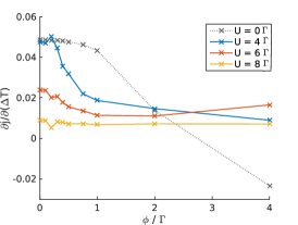
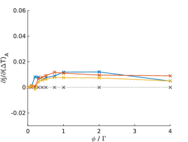
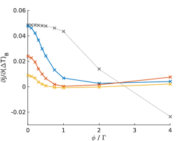
Figure 1: (Color online) Thermoelectric response for $V_{G}=\Gamma$ and for various values of the interaction strength $U$. The first panel depicts $\partial{j}/\partial(\Delta{T})$, Eq. (14), and the second and third panel the two parts of Eqs. (15) and (16). See App. A for a discussion on the accuracy of the numerical derivative.

In order to determine the nonequilibrium self-energy $\underline{\Sigma}(\omega)$ we here use the so-called auxiliary master equation approach (AMEA), as previously introduced in Refs. ar.kn.13, ; do.nu.14, and in its recent MPS implementation Ref. do.ga.15, . The basic principle of the approach is to map the original nonequilibrium (or equilibrium) impurity problem onto an auxiliary one, in which the bath is modeled by a small number $N_{B}$ of bath sites and additional Markovian environments. By this, a finite open quantum system described by a Lindblad equation is obtained, which can be solved accurately by numerical techniques. The mapping procedure relies on the condition to represent the original hybridization function as accurately as possible by the auxiliary one. A similar idea is commonly used in the context of dynamical mean field theory me.vo.89 ; ge.ko.92 . However, in order to be able to address nonequilibrium situations it is necessary to fit not only the retarded but also the Keldysh component, and therefore to construct an auxiliary hybridization with a continuous spectrum. The AMEA approach is conveniently formulated in terms of Keldysh Green’s functions sc.61 ; ka.ba.62 ; ke.65 ; ha.ja.98 ; ra.sm.86 ; st.le.13 , and particularly suited to treat steady state situations. Time-dependent problems are also accessible in principle, but go beyond the scope of the present work.

AMEA provides an accurate approximation for the impurity self-energy $\underline{\Sigma}(\omega)$, for details on the method we refer to Ref. do.ga.15, . The accuracy is hereby controlled by the quality of the mapping procedure and can be systematically improved by increasing $N_{B}$, the convergence being exponential in $N_{B}$ do.ga.15 ; do.so.16u . In practice, of course, finite values for $N_{B}$ have to be chosen and with that techniques we are currently able to consider as many as $N_{B}\approx 10-20$. The calculations in Ref. do.ga.15, demonstrated that these values allow for very accurate results. All of the calculations presented below are for $N_{B}=14$.

For the calculation of thermoelectric properties one needs to consider systems away from particle-hole symmetry. In our previous calculations in Ref. ar.kn.13, ; do.nu.14, ; do.ga.15, we treated particle-hole symmetric situations only. However, this was done for convenience and is by no means a restriction of the method. The difference is that for $V_{G}\neq 0$ two independent Green’s functions have to be computed in the many-body solution and that twice as many fit parameters must be considered in the mapping procedure. Both aspects require increased computational resources, mainly due to the many-body calculation, but no essential conceptual modifications. The differential quantities $\partial{j}/\partial(\Delta{T})$ are estimated by finite differences, see App. A for more details on the implementation.

III Results

We start by investigating the current response $\partial{j}/\partial(\Delta{T})$ of the nonequilibrium SIAM to an infinitesimal temperature difference $d(\Delta{T})$. We are interested, in particular, in the nonequilibrium behavior as a function of bias voltage $\phi$. For all calculations we used an average temperature $T=0.1\,\Gamma$, which, for $U=6\,\Gamma$ and $V_{G}\approx 2\,\Gamma$, corresponds to the point at which $\partial{j}/\partial(\Delta{T})$ as function of $T$ has a maximum below $T_{K}$. This is determined from an equilibrium NRG calculation  endnote2 , see inset of the third panel of Fig. 3.

In Fig. 1 we analyze the general behavior of $\partial{j}/\partial(\Delta{T})$ as a function of $\phi$ as determined by Eq. (14) together with its two contributions Eqs. (15) and (16), for different values of $U$ at a gate voltage $V_{G}=\Gamma$. In the noninteracting case, a plateau up to $\phi=V_{G}$ precedes the decrease of $\partial{j}/\partial(\Delta{T})$ as a function of $\phi$ . In this case only the second term $\partial{j}/\partial(\Delta{T})$_B contributes since the lead density of states, and thus the noninteracting spectral function $A(\omega)$, is independent of $\phi$ and $T$. As a consequence, according to Eq. (16), for $U=0$ we have that $\partial{j}/\partial(\Delta{T})$ just measures the asymmetry of the equilibrium $A(\omega)$ at $\omega=\pm\phi/2$.

For a finite value of $U\geq 4\,\Gamma$ in the Kondo regime, the results change significantly. The current response $\partial{j}/\partial(\Delta{T})$ is positive for all $\phi$ and decreases much faster as a function of $\phi$, with a dependence that resembles the one of $\partial{j}/\partial\phi$, see e.g. Refs. do.ga.15, ; pl.sc.12, ; an.08, ; ha.he.07, ; co.gu.14, ; ro.pa.03, ; ke.05, ; sc.re.09, . However, in contrast to the conductance, in this case the relevant energy scale controlling the decrease can not be identified with $T_{K}$. In particular, it does not depend on $U$ and appears to be proportional to $\Gamma$. This agrees with the findings in Ref. co.zl.10, and with the results below. We note the functional behavior of the two contributions $\partial{j}/\partial(\Delta{T})$_A and $\partial{j}/\partial(\Delta{T})$_B is very different, as shown in the second and third panel of Fig. 1. While $\partial{j}/\partial(\Delta{T})$_B decreases with $\phi$ (being maximal for $\phi=0$) and strongly depends on the interaction, $\partial{j}/\partial(\Delta{T})$_A in contrast, exhibits a similar behavior for all values of $U$: starting from zero, $\partial{j}/\partial(\Delta{T})$_A increases with applied bias and saturates at $\phi\approx\Gamma$. For $U=8\,\Gamma$ the two contributions compensate each other yielding a nearly $\phi$-independent $\partial{j}/\partial(\Delta{T})$.

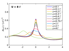
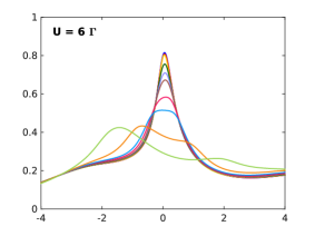
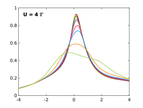
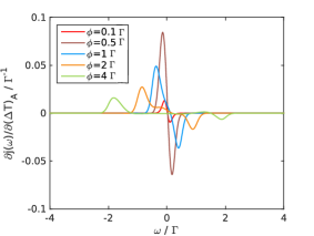
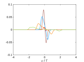
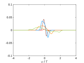
Figure 2: (Color online) Spectral functions $A(\omega)$ for $\Delta{T}=0$ on top and of the integrand of Eq. (15) $\partial j(\omega)/\partial(\Delta{T})$ at the bottom, which is proportional to $\partial A(\omega)/\partial(\Delta{T})$. The results are shown for the same parameters as in Fig. 1, i.e. on the left for $U=8\,\Gamma$, in the center for $U=6\,\Gamma$ and on the right for $U=4\,\Gamma$, with $V_{G}=\Gamma$ in all cases.

In order to gain a more detailed understanding of this behavior we analyze the frequency dependence of the spectral function as well as of the integrand determining $\partial{j}/\partial(\Delta{T})$. The nonequilibrium spectral functions for $\Delta{T}=0$, which determine the second contribution $\partial{j}/\partial(\Delta{T})$_B, are shown in the upper panels of Fig. 2. We observe a pronounced Kondo peak at $\phi=0$ for all values of $U$. For the results depicted in Fig. 2 the temperature is fixed to $T=0.1\,\Gamma$ and $U$ decreases from left to right. Hence the ratio $T/T_{K}$ decreases from left to right, resulting in an increasing height of the Kondo peak. Moreover, it appears that for the smallest value of the interaction the peak is rather broad as it is not well separated from the lower Hubbard band  as compared to larger $U$. The low-energy details are less smeared out for $U\geq 6\,\Gamma$ for which a splitting of the Kondo resonance into two peaks is clearly visible for sufficiently large $\phi$. In contrast to the particle-hole symmetric case (s. Ref. do.ga.15, ) the splitting is asymmetric in presence of a finite gate voltage. According to Eq. (16), the asymmetry of $A(\omega)$ at $\omega=\mu_{L/R}$ determines $\partial{j}/\partial(\Delta{T})$_B.

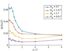
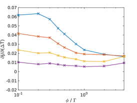
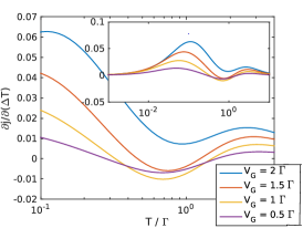
Figure 3: (Color online) Thermoelectric response $\partial{j}/\partial(\Delta{T})$ as a function of bias voltage $\phi$ in the first panel (in the second on a semi-logarithmic scale), and in the third for $\phi=0$ as a function of $T$. All calculations are for $U=6\,\Gamma$ and for various $V_{G}$. The equilibrium values on the right are obtained from NRG  endnote2 . The inset depicts the behavior for a larger temperature range.

In the lower panels of Fig. 2 we show results for the response of the spectral function to an infinitesimal temperature difference, more specifically the integrand $\partial j(\omega)/\partial(\Delta{T})_{A}$ of Eq. (15) which is proportional to $\partial A(\omega)/\partial(\Delta{T})$ (evaluated numerically) times the transport window $f_{R}(\omega)-f_{L}(\omega)$. $\partial j(\omega)/\partial(\Delta{T})_{A}$ is maximal for $\phi\sim 0.5\,\Gamma$ and vanishes in the limit $\phi\to 0$ due to the narrowing transport window. The main characteristic features are a positive peak at $\omega\approx-\phi/2$ and a negative one at $\omega\approx\phi/2$, which appear in correspondence of the position of the leads’ chemical potentials and thus of the split Kondo peaks. Hence the Kondo peaks strongly affect the response $\partial A(\omega)/\partial(\Delta{T})$ to a temperature difference. In the limit of large $\phi$ and $U$ a simple picture emerges: the dominating effect of $\Delta{T}$ is that the split Kondo peaks are asymmetrically enhanced or suppressed. This effect can be clearly seen for $U=8\,\Gamma$ and $\phi=4\,\Gamma$, for instance, where $\partial j(\omega)/\partial(\Delta{T})_{A}$ exhibits only two peaks at $\omega\approx\pm\phi/2$ and no response in the region in between. The sign of the two peaks is determined by the direction in which the temperature difference is applied. Since we considered $T_{L}=T-\Delta{T}/2$ and $T_{R}=T+\Delta{T}/2$, analogously to $\mu_{L}=-\phi/2$ and $\mu_{R}=+\phi/2$, it is intuitive that the Kondo peak at $\omega<0$ is enhanced and the one at $\omega>0$ is suppressed. For lower values of the interaction strength the behavior is more complex since the split Kondo peaks are less pronounced and merge with the Hubbard bands already for rather small values of $\phi$. In all cases, the overall sign when integrating $\partial j(\omega)/\partial(\Delta{T})_{A}$ is positive (see also Fig. 1), since for $V_{G}>0$ the Kondo peak at $\omega<0$ is enhanced by the proximity of the lower Hubbard band.

It is interesting to note that the nearly constant $\partial{j}/\partial(\Delta{T})$ for $\phi\gtrsim\Gamma$ and $U\geq 6\,\Gamma$, as observed in Fig. 1, is dominated by the response of the split Kondo peaks. As discussed above, both contributions $\partial{j}/\partial(\Delta{T})$_B and $\partial{j}/\partial(\Delta{T})$_A are in this parameter regime essentially determined by the asymmetry of $A(\omega)$ and its response at $\omega=\pm\phi/2$, which corresponds to the positions of the split Kondo peaks.

In general, the Kondo resonance is suppressed by both a finite temperature $T$ and a bias voltage $\phi$, otherwise the two external parameters act in a very different manner: a finite $T$ (at $\phi=0$) induces a lowering of the Kondo resonance peak height, whereas a finite $\phi$ (at $T<T_{K}$) in addition splits the peak in two, see also upper panel of Fig. 2. From previous results it is known that the differential conductance $\partial{j}/\partial\phi$ is not affected by this difference, since it shows qualitatively the same functional dependence on $T$ as on $\phi$ pl.sc.12 ; sm.gr.11 ; sm.gr.13 ; mu.bo.13 ; re.pl.14 ; mo.mo.15 ; an.do.16 . The question arises whether this holds true also for $\partial{j}/\partial(\Delta{T})$.

To address this issue, we show results for $\partial{j}/\partial(\Delta{T})$ as a function of $\phi$ and $T$ in Fig. 3, for $U=6\,\Gamma$ and for various $V_{G}$. The nonequilibrium calculations were obtained with AMEA and the equilibrium ones with NRG  endnote2 . Already from the equilibrium behavior displayed in the inset on the right one notices that the temperature dependence of $\partial{j}/\partial(\Delta{T})$ is quite involved. Apart from $V_{G}=2\,\Gamma$ all curves exhibit sign changes  endnote6 . These findings are in agreement with the results reported in Ref. co.zl.10, , where the Seebeck coefficient ${\cal S}$, i.e. Eq. (13) for $j=0$, was investigated in detail for $\phi=0$. Note that the sign of $\partial{j}/\partial(\Delta{T})$ determines the sign of ${\cal S}$. In general, $\partial{j}/\partial(\Delta{T})$ vanishes for $V_{G}\to 0$ and also for $T\to 0$. The latter can be understood from a Sommerfeld expansion of Eq. (16) co.zl.10 ; ki.za.12 which yields for $\partial{j}/\partial(\Delta{T})$ a linear behavior in $T$ for $T\to 0$. The vanishing $\partial{j}/\partial(\Delta{T})$ for small $T$ can be observed in the inset of the right panel in Fig. 3. In contrast, the left panel reveals that for $\phi\to 0$ the thermoelectric property $\partial{j}/\partial(\Delta{T})$ approaches a finite, even $V_{G}$-dependent value. This is a first indication of the different dependence of $\partial{j}/\partial(\Delta{T})$ on temperature and on bias voltage.

In order to investigate the $\phi$-dependence of $\partial{j}/\partial(\Delta{T})$ in the Kondo regime we consider $T=0.1\,\Gamma$, which corresponds approximately to the position of the maximum of $\partial{j}/\partial(\Delta{T})$ as a function of temperature (for $T<T_{K}$) (see inset in right panel). The results for the dependence on $\phi$ are shown in the first two panels of Fig. 3. One can see that the characteristic scale that governs the decrease of $\partial{j}/\partial(\Delta{T})$ with $\phi$ is $\Gamma$ and not the Kondo temperature $T_{K}$. The appearance of additional energy scales proportional to $\Gamma$ has been also found in the equilibrium thermoelectric properties of the SIAM co.zl.10 . A comparison of the functional dependence of $\partial{j}/\partial(\Delta{T})$ on $\phi/\Gamma$ (for $T=0.1\,\Gamma$) and on $T/\Gamma$ (for $\phi=0$) is provided in the second and third panel of Fig. 3, both with logarithmic abscissa starting at $10^{-1}$. We note that for $T=0.1\,\Gamma$ and $\phi=0$ the results obtained from AMEA and from NRG agree very well. The equilibrium ($T$-dependent) and nonequilibrium ($\phi$-dependent) data behave similarly only for large values of the gate voltage ($V_{G}=2\,\Gamma$), while they deviate from each other as a function of $\phi$ or $T$ for small $V_{G}\approx\Gamma$. In particular, in nonequilibrium the decrease of $\partial{j}/\partial(\Delta{T})$ with $\phi$ is followed by a saturation to a finite (positive) value, whereas in equilibrium the oscillating behavior as a function of $T$ exhibits also sign changes. As a consequence, the resulting thermoelectric response of a SIAM in the Kondo regime is characterized by pronounced differences.

We note that the quantity $\partial{j}/\partial(\Delta{T})$ is rather sensitive to details of the spectral function $A(\omega)$. Differently to $\partial{j}/\partial\phi$, which involves an effective averaging over the transport window, $\partial{j}/\partial(\Delta{T})$ is mainly determined by the response at $\omega=\pm\phi/2$, as discussed above. This explains the observed differences in the behavior of $\partial{j}/\partial(\Delta{T})$ with respect to $\partial{j}/\partial\phi$, between the dependence on $T$ in equilibrium and the one of $\phi$ in nonequilibrium.

Finally, We stress that, while we here restrict to linear order in $\Delta{T}$ the present method can evaluate nonequilibrium properties for any finite $\Delta{T}$ (and $\phi$). In addition, we estimated up to what $\Delta{T}$ the linear regime is valid by computing a $\Delta{T}_{val}$ for which the second order term in $\Delta{T}$ becomes of the same order as the first order correction (we have an estimate for the second derivative of $j$ with respect to $\Delta{T}$ from finite differences). We get values of $\Delta{T}_{val}/T_{K}={0.4,1.5,0.7}$ for $\phi={0.1\Gamma,0.4\Gamma,2\Gamma}$, for the exemplary case $U=6\ \Gamma$ and $V_{G}=\Gamma$. Therefore, roughly for $\Delta{T}$ up to $T_{K}$ the linear regime is accurate.

In view of sensing applications we conclude that the response is maximal in proximity of the linear response regime for $\phi=0$ and moreover, that fairly large gate voltages are advantageous. As illustrated by the results for $V_{G}=2\,\Gamma$ considered here, a small plateau develops in the region up to $\phi\approx 0.3\,\Gamma$ in which $\partial{j}/\partial(\Delta{T})$ is nearly constant. In general, this might be achieved by tuning the system to a temperature just below the maximum of $\partial{j}/\partial(\Delta{T})$ at $\phi=0$. However, further studies including also asymmetric couplings to the leads are required to fully assess the potential of quantum dot devices for nanoscale sensing applications.

IV Conclusions

In the present work we computed the nonequilibrium spectral and thermoelectric transport properties of a quantum dot modeled by a SIAM in presence of both, an external bias voltage $\phi$ and a temperature difference $\Delta{T}$ between the two leads. In particular, we focused on the differential response of the current to a temperature gradient $\partial{j}/\partial(\Delta{T})$ in the nonequilibrium Kondo regime ($\phi\neq 0$ and $T<T_{K}$), for the case of an infinitesimal temperature difference $d(\Delta{T})$. When compared to the results for the differential conductance $\partial{j}/\partial\phi$ known from previous studies pl.sc.12 ; sm.gr.11 ; sm.gr.13 ; mu.bo.13 ; re.pl.14 ; mo.mo.15 ; an.do.16 , we find that $\partial{j}/\partial(\Delta{T})$ exhibits a more complex behavior. On the one hand, the equilibrium and nonequilibrium properties turn out to be quite different, i.e. whether one monitors $\partial{j}/\partial(\Delta{T})$ as a function of $T$ or of $\phi$, and on the other hand, the relevant low-energy scales are more involved. $\partial{j}/\partial(\Delta{T})$ reveals a rapid decrease with increasing $\phi$, similar to $\partial{j}/\partial\phi$, however, governed by a scale determined by the coupling strength $\Gamma$ and not $T_{K}$. This finding is consistent with equilibrium results reported in Ref. co.zl.10, .

A more detailed understanding is gained by inspecting the different contributions to $\partial{j}/\partial(\Delta{T})$, and especially by analyzing the spectral function $A(\omega)$ and its frequency-resolved response to $\Delta T$. Here, we presented a systematic study for various values of the interaction strength $U$ and gate voltages $V_{G}$. In the regime of strong interactions and sufficiently large bias voltages we provided a simple physical picture, based on the asymmetric suppression or enhancement of the split Kondo peak. A temperature reduction of $\Delta{T}$/2 in one lead and the respective increase in the other one induces an asymmetric response of the two Kondo peaks. This characteristic nonequilibrium feature lead to the qualitatively different behavior of $\partial{j}/\partial(\Delta{T})$ as a function of $T$ or of $\phi$. By extending our previous results do.ga.15 to non-particle-hole symmetric situations we were able to accurately resolve the asymmetric splitting of the Kondo peak in $A(\omega)$ with increasing bias voltage. We note that in contrast to other previous works (see e.g. Ref. du.le.13, ), we here report a clear observation of this splitting, which was not accessible before, and its evolution with increasing values of $U$.

On the whole, one can conclude that $\partial{j}/\partial(\Delta{T})$ is more sensitive to details in the spectral function $A(\omega)$ than the differential conductance $\partial{j}/\partial\phi$. Besides the fundamental interest, the findings reported here may be of value to assess the potential of quantum dots as possible nanoscale temperature sensors.

Appendix A Numerical differentiation of the spectral function

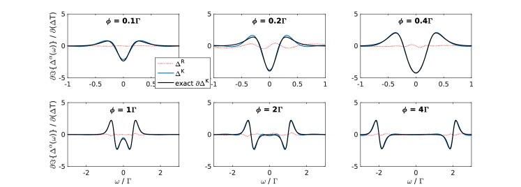
Figure 4: (Color online) Numerically estimated differentials $\partial\underline{\Delta}_{\mathrm{aux}}(\omega)/\partial(\Delta{T})$, labeled by $\Delta^{\alpha}(\omega)$ with $\alpha=R,K$, together with the analytical expressions given in Eqs. (6) and (11). Only the exact $\partial\Delta^{K}(\omega)/\partial(\Delta{T})$ is plotted since $\partial\Delta^{R}(\omega)/\partial(\Delta{T})=0$. Especially for $\phi=0.2\,\Gamma$ larger errors occur and $\partial\Delta^{R}(\omega)/\partial(\Delta{T})$ is clearly nonzero.

In order to evaluate Eq. (14) in nonequilibrium $\phi\neq 0$ one needs to calculate $\partial\mathcal{T}(\omega)/\partial(\Delta{T})$ in Eq. (15) numerically. Details on this are given here.

AMEA consists of two major steps: (i) the mapping procedure, and (ii) the many-body solution. In (i) we optimize all available bath parameters in the auxiliary system for a given number of bath sites $N_{B}$ in order to reproduce the hybridization function of the physical system $\underline{\Delta}(\omega)$, Eq. (11), by the auxiliary one $\underline{\Delta}_{\mathrm{aux}}(\omega)$ as accurately as possible. This is done through a fit on the real $\omega$-axis and with a parallel tempering (PT) routine ea.de.05 ; hu.ne.96 , see Ref. do.ga.15, . We thus aim at solving a global optimization problem in the fit. Once the optimal bath parameters are obtained we thereafter proceed to step (ii) and treat the many-body problem. In Ref. do.ga.15, we presented a solution strategy based on matrix product states, which we also make use of in the present work.

$f^{\prime}(\Delta T)\big{|}_{\Delta T=0}:=\partial\mathcal{T}(\omega,\Delta T)/\partial(\Delta{T})\big{|}_{\Delta T=0}$ is estimated by finite differences. First we compute for a certain $\phi$ the fit for the particle-hole symmetric case at $\Delta{T}=0$, in the manner just described above (see also Ref. do.ga.15, ). Thereafter, we introduce a small finite temperature difference $\Delta{T}\approx T/10$, start the fit from the bath parameters obtained for $\Delta{T}=0$ and optimize only locally . By this, the fit for $\Delta{T}\neq 0$ is close in parameter space to the one for $\Delta{T}=0$ and we can thus estimate the linear response with respect to $\Delta{T}$. In order to approximate a derivative by finite differences accurately it would be appropriate, in principle, to consider various stencils with varying values of $\Delta{T}$. Since this would require a major computational effort in the many-body calculation we consider here for simplicity only two values $\Delta{T}=\pm T/10$. Note further that these two fits are connected by a particle-hole transformation. The derivative $f^{\prime}(\Delta T)\big{|}_{\Delta T=0}$ is approximated by the central finite difference, i.e. based on $\Delta{T}=\pm T/10$. Together with the computation for $\Delta{T}=0$ this amounts to three many-body calculations for a certain $\phi$ and $T$.

Already on the level of the mapping procedure, i.e. before solving the many-body problem, one can check how well the finite difference approach works with the chosen $N_{B}$ and $\Delta{T}$. For this we compute the derivative of the hybridization function. The derivative of the physical hybridization function Eq. (11) of the original impurity problem can be carried out analytically. The temperature difference enters only through the Keldysh component, so that $\partial\Delta^{R}(\omega)/\partial(\Delta{T})=0$ and the expression for $\partial\Delta^{K}(\omega)/\partial(\Delta{T})$ is obtained by differentiating the Fermi functions in Eqs. (11) and (6). A comparison of the estimated derivatives versus the exact ones is shown in Fig. 4 for a representative set of bias voltages. Overall, a good agreement is found. Larger differences occur for instance at $\phi=0.2\,\Gamma$, where the retarded part is clearly nonzero and also the Keldysh part exhibits more deviations. Judging from such an analysis and from comparing the values of the forward, backward and central difference approximations of $f^{\prime}(\Delta T)\big{|}_{\Delta T=0}$, we can state that the presented data points for the numerical derivatives in Fig. 1 and Fig. 3 are less reliable for $\phi=0.2\,\Gamma$. For larger values of $\phi$ and for $\phi\leq 0.1\,\Gamma$ results are more accurate. A rigorous quantitative estimate of the error originating from the numerical derivative would require a more expensive numerical analysis. On the contrary, the computed spectral functions in Fig. 2 can be regarded to have a high accuracy.  This shows that the computation of derivatives magnifies small inaccuracies of the mapping procedure, which are present for a certain finite value of $N_{B}$.

References

- (1) L. I. Glazman and M. E. Raikh, JETP Lett. 47, 452 (1988).
- (2) T. K. Ng and P. A. Lee, Phys. Rev. Lett. 61, 1768 (1988).
- (3) D. Goldhaber-Gordon, H. Shtrikman, D. Mahalu, D. Abusch-Magder, U. Meirav, and M. Kastner, Nature (London) 391, 156 (1998).
- (4) S. M. Cronenwett, T. H. Oosterkamp, and L. P. Kouwenhoven, Science 281, 540 (1998).
- (5) J. Schmid, J. Weis, K. Eberl, and K. v. Klitzing, Physica B (Amsterdam) 256, 182 (1998).
- (6) A. Rosch, J. Paaske, J. Kroha, and P. Wölfle, Phys. Rev. Lett. 90, 076804 (2003).
- (7) S. Kehrein, Phys. Rev. Lett. 95, 056602 (2005).
- (8) H. Schoeller and F. Reininghaus, Phys. Rev. B 80, 045117 (2009); H. Schoeller and F. Reininghaus, Phys. Rev. B 80, 209901(E)(2009).
- (9) G. D. Mahan and J. O. Sofo, Proc. Natl. Acad. Sci. USA 93, 7436 (1996).
- (10) F. Simmel, R. H. Blick, J. P. Kotthaus, W. Wegscheider, and M. Bichler, Phys. Rev. Lett. 83, 804 (1999).
- (11) S. De Franceschi, S. Sasaki, J. M. Elzerman, W. G. van der Wiel, S. Tarucha, and L. P. Kouwenhoven, Phys. Rev. Lett. 86, 878 (2001).
- (12) J. Paaske, A. Rosch, P. Wölfle, N. Mason, C. M. Marcus, and J. Nygard, Nat. Phys. 2, 460 (2006).
- (13) C. W. J. Beenakker and A. A. M. Staring, Phys. Rev. B 46, 9667 (1992).
- (14) D. M. Zumbühl, C. M. Marcus, M. P. Hanson, and A. C. Gossard, Phys. Rev. Lett. 93, 256801 (2004).
- (15) S. Sapmaz, P. Jarillo-Herrero, J. Kong, C. Dekker, L. P. Kouwenhoven, and H. S. J. van der Zant, Phys. Rev. B 71, 153402 (2005).
- (16) A. K. Hüttel, B. Witkamp, M. Leijnse, M. R. Wegewijs, and H. S. J. van der Zant, Phys. Rev. Lett. 102, 225501 (2009).
- (17) F. A. Zwanenburg, A. S. Dzurak, A. Morello, M. Y. Simmons, L. C. L. Hollenberg, G. Klimeck, S. Rogge, S. N. Coppersmith, and M. A. Eriksson, Rev. Mod. Phys. 85, 961 (2013).
- (18) E. A. Osorio, K. O’Neill, N. Stuhr-Hansen, O. F. Nielsen, T. Bjørnholm, and H. S. J. van der Zant, Adv. Mater. 19, 281 (2007).
- (19) A. J. Heinrich, J. A. Gupta, C. P. Lutz, and D. M. Eigler, Science 306, 466 (2004).
- (20) J. E. Grose, E. S. Tam, C. Timm, M. Scheloske, B. Ulgut, J. J. Parks, H. D. Abruna, W. Harneit, and D. C. Ralph, Nat. Mater. 7, 884 (2008).
- (21) J. J. Parks, A. R. Champagne, G. R. Hutchison, S. Flores-Torres, H. D. Abruña, and D. C. Ralph, Phys. Rev. Lett. 99, 026601 (2007).
- (22) A. S. Zyazin, J. W. G. van den Berg, E. A. Osorio, H. S. J. van der Zant, N. P. Konstantinidis, M. Leijnse, M. R. Wegewijs, F. May, W. Hofstetter, C. Danieli, and A. Cornia, Nano Lett. 10, 3307 (2010).
- (23) S. Loth, K. von Bergmann, M. Ternes, A. F. Otte, C. Lutz, and A. Heinrich, Nat. Phys. 6, 340 (2010).
- (24) T. Jespersen, K. Grove-Rasmussen, J. Paaske, K. Muraki, T. Fujisawa, J. Nygard, and K. Flensberg, Nat. Phys. 7, 348 (2011).
- (25) R. Scheibner, H. Buhmann, D. Reuter, M. N. Kiselev, and L. W. Molenkamp, Phys. Rev. Lett. 95, 176602 (2005).
- (26) P. Reddy, S.-Y. Jang, R. A. Segalman, and A. Mujamdar, Science 315, 1568 (2007).
- (27) K. Baheti, J. A. Malen, P. Doak, P. Reddy, S.-Y. Jang, T. D. Tilley, A. Mujamdar, and R. A. Segalman, Nano Lett. 8, 715 (2008).
- (28) J. R. Widawsky, P. Darancet, J. B. Neaton, and L. Venkataraman, Nano Lett. 12, 354 (2012).
- (29) R. Temirov, A. Lassise, F. B. Anders, and F. S. Tautz, Nanotechnology 19, 065401 (2008).
- (30) W. Lee, K. Kim, W. Jeong, L. A. Zotti, F. Pauly, J. C. Cuevas, and P. Reddy, Nature (London) 498, 209 (2013).
- (31) Y. Kim, W. Jeong, K. Kim, W. Lee, and P. Reddy, Nat. Nanotechnol. 9, 881 (2014).
- (32) N. M. Gergs, C. B. M. Hörig, M. R. Wegewijs, and D.Schuricht, Phys. Rev. 91, 201107(R) (2015).
- (33) F. B. Anders, Phys. Rev. Lett. 101, 066804 (2008).
- (34) R. E. V. Profumo, C. Groth, L. Messio, O. Parcollet, and X. Waintal, Phys. Rev. B 91, 245154 (2015).
- (35) R. Härtle, G. Cohen, D. R. Reichman, and A. J. Millis, Phys. Rev. B 92, 085430 (2015).
- (36) F. Güttge, F. B. Anders, U. Schollwöck, E. Eidelstein, and A. Schiller, Phys. Rev. B 87, 115115 (2013).
- (37) S. Andergassen, V. Meden, H. Schoeller, J. Splettstoesser, and M. R. Wegewijs, Nanotechnology 21, 272001 (2010).
- (38) A. Dorda, M. Nuss, W. von der Linden, and E. Arrigoni, Phys. Rev. B 89, 165105 (2014).
- (39) A. Dorda, M. Ganahl, H. G. Evertz, W. von der Linden, and E. Arrigoni, Phys. Rev. B 92, 125145 (2015).
- (40) S. Hershfield, Phys. Rev. Lett. 70, 2134 (1993).
- (41) P. Mehta and N. Andrei, Phys. Rev. Lett. 96, 216802 (2006).
- (42) N. S. Wingreen and Y. Meir, Phys. Rev. B 49, 11040 (1994).
- (43) E. Lebanon and A. Schiller, Phys. Rev. B 65, 035308 (2001).
- (44) A. Rosch, J. Kroha, and P. Wölfle, Phys. Rev. Lett. 87, 156802 (2001).
- (45) J. König, J. Schmid, H. Schoeller, and G. Schön, Phys. Rev. B 54, 16820 (1996).
- (46) T. Fujii and K. Ueda, Phys. Rev. B 68, 155310 (2003).
- (47) S. Smirnov and M. Grifoni, Phys. Rev. B 84, 125303 (2011).
- (48) S. Smirnov and M. Grifoni, New Journal of Physics 15, 073047 (2013).
- (49) C. Jung, A. Lieder, S. Brener, H. Hafermann, B. Baxevanis, A. Chudnovskiy, A. Rubtsov, M. Katsnelson, and A. Lichtenstein, Ann. Phys. 524, 49 (2012).
- (50) N. Shah and A. Rosch, Phys. Rev. B 73, 081309 (2006).
- (51) P. Fritsch and S. Kehrein, Phys. Rev. B 81, 035113 (2010).
- (52) S. G. Jakobs, M. Pletyukhov, and H. Schoeller, Phys. Rev. B 81, 195109 (2010).
- (53) R. B. Saptsov and M. R. Wegewijs, Phys. Rev. B 86, 235432 (2012).
- (54) F. Reininghaus, M. Pletyukhov, and H. Schoeller, Phys. Rev. B 90, 085121 (2014).
- (55) S. Andergassen, D. Schuricht, M. Pletyukhov, and H. Schoeller, AIP Conference Proceedings 1633, 213 (2014).
- (56) F. Heidrich-Meisner, A. E. Feiguin, and E. Dagotto, Phys. Rev. B 79, 235336 (2009).
- (57) A. Holzner, I. P. McCulloch, U. Schollwöck, J. von Delft, and F. Heidrich-Meisner, Phys. Rev. B 80, 205114 (2009).
- (58) M. Nuss, M. Ganahl, H. G. Evertz, E. Arrigoni, and W. von der Linden, Phys. Rev. B 88, 045132 (2013).
- (59) M. Nuss, M. Ganahl, E. Arrigoni, W. von der Linden, and H. G. Evertz, Phys. Rev. B 91, 085127 (2015).
- (60) S. Schmitt and F. B. Anders, Phys. Rev. Lett. 107, 056801 (2011).
- (61) A. Jovchev and F. B. Anders, Phys. Rev. B 87, 195112 (2013).
- (62) P. Werner, T. Oka, M. Eckstein, and A. J. Millis, Phys. Rev. B 81, 035108 (2010).
- (63) M. Nuss, C. Heil, M. Ganahl, M. Knap, H. G. Evertz, E. Arrigoni, and W. von der Linden, Phys. Rev. B 86, 245119 (2012).
- (64) J. E. Han and R. J. Heary, Phys. Rev. Lett. 99, 236808 (2007).
- (65) G. Cohen, E. Gull, D. R. Reichman, and A. J. Millis, Phys. Rev. Lett. 112, 146802 (2014).
- (66) M. Pletyukhov and H. Schoeller, Phys. Rev. Lett. 108, 260601 (2012).
- (67) E. Munoz, C. J. Bolech, and S. Kirchner, Phys. Rev. Lett. 110, 016601 (2013).
- (68) E. Arrigoni, M. Knap, and W. von der Linden, Phys. Rev. Lett. 110, 086403 (2013).
- (69) I. Titvinidze, A. Dorda, W. von der Linden, and E. Arrigoni, Phys. Rev. B 92, 245125 (2015).
- (70) A. Dorda, I. Titvinidze, and E. Arrigoni, J. Phys.: Conf. Ser. 696, 012003 (2016).
- (71) T.-S. Kim and S. Hershfield, Phys. Rev. Lett. 88, 136601 (2002).
- (72) T. A. Costi and V. Zlatic, Phys. Rev. B 81, 235127 (2010).
- (73) M. Turek and K. A. Matveev, Phys. Rev. B 65, 115332 (2002).
- (74) J. Koch, F. von Oppen, Y. Oreg, and E. Sela, Phys. Rev. B 70, 195107 (2004).
- (75) B. Kubala and J. Kon̈ig, Phys. Rev. B 73, 195316 (2006).
- (76) T. A. Costi and A. C. Hewson, J. Phys.: Condens. Matter 5, L361 (1993).
- (77) T. Rejec, R. Zitko, J. Mravlje, and A. Ramsak, Phys. Rev. B 85, 085117 (2012).
- (78) D. M. Kennes, D. Schuricht, and V. Meden, Europhys. Lett. 102, 57003 (2013).
- (79) B. Kubala, J. König, and J. Pekola, Phys. Rev. Lett. 100, 066801 (2008);
- (80) P. Murphy, S. Mukerjee, and J. E. Moore, Phys. Rev. B 78, 161406(R) (2008);
- (81) S. Andergassen, T. A. Costi, and V. Zlatic, Phys. Rev. B 84, 241107(R) (2011).
- (82) J. Azema, A.-M. Daré, S. Schäfer, and P. Lombardo, Phys. Rev. B 86, 075303 (2012);
- (83) P. S. Cornaglia, G. Usaj, and C. A. Balseiro, ibid. 86, 041107(R) (2012);
- (84) P. Roura-Bas, L. Tosi, A. A. Aligia, and P. S. Cornaglia, ibid. 86, 165106 (2012);
- (85) S. Hong, P. Ghaemi, J. E. Moore, and P. W. Phillips, Phys. Rev. B 88, 075118 (2013);
- (86) L.Z. Ye, D. Hou, R. Wang, D. Cao, X. Zheng, and Y. J. Yan, Phys. Rev. B 90, 165116 (2014);
- (87) R. Sanchez, B. Sothmann, A. N. Jordan, and M. Büttiker, New J. Phys. 15, 125001 (2013);
- (88) S. F. Svensson, E. A. Hoffmann, N. Nakpathomkun, P. M. Wu, H. Xu, H. A. Nilsson, D. Sánchez, V. Kashcheyevs, and H. Linke, New J. Phys. 15, 105011 (2013);
- (89) R. Zitko, J. Mravlje, A. Ramsak, and T. Rejec, New J. Phys. 15, 105023 (2013).
- (90) M. Leijnse, M. R. Wegewijs, and K. Flensberg, Phys. Rev. B 82, 045412 (2010).
- (91) M. Esposito, K. Lindenberg, and C. van den Broeck, Europhys. Lett. 85, 60010 (2009).
- (92) H. Wang, G. Wu, Y. Fu, and D. Chen, J. Appl. Phys. 111, 094318 (2012).
- (93) M. Galperin, M. A. Ratner, and A. Nitzan, J. Phys.: Condens. Matter 19, 103201 (2007).
- (94) R. Lopez and D. Sanchez, Phys. Rev. B 88, 045129 (2013).
- (95) R. S. Whitney, Phys. Rev. B 88, 064302 (2013).
- (96) S. Fahlvik Svensson, E. A. Hoffmann, N. Nakpathomkun, P. M. Wu, H. Q. Xu, H. A. Nilsson, D. Sanchez, V. Kashcheyevs, and H. Linke, New J. Phys. 15, 105011 (2013).
- (97) L. A. Zotti, M. Bürkle, F. Pauly, W. Lee, W. J. K. Kim, Y. Asai, P. Reddy, and J. C. Cuevas, New J. Phys. 16, 015004 (2014).
- (98) A. V. Kretinin, H. Shtrikman, and D. Mahalu, Phys. Rev. B 85, 201301(R) (2012).
- (99) S. Kirchner, F. Zamani, and E. Muñoz, chapter contributed to ”New Materials for Thermoelectric Applications: Theory and Experiment”, Springer Series: NATO Science for Peace and Security Series - B: Physics and Biophysics, V. Zlatic (Editor), A. Hewson (Editor) (2012).
- (100) T. C. Harman, P. J. Taylor, M. P. Walsh, and B. E. LaForge, Science 297, 2229 (2002).
- (101) A. Majumdar, Science 303, 777 (2004).
- (102) T. E. Humphrey, R. Newbury, R. P. Taylor, and H. Linke, Phys. Rev. Lett. 89, 116801 (2002).
- (103) G. D. Mahan, B. Sales, and J. Sharp, Phys. Today 50, 42 (1997).
- (104) F. Giazotto, T. T. Heikkilä, A. Luukanen, A. M. Savin, and J. P. Pekola, Rev. Mod. Phys. 78, 217 (2006).
- (105) J. K. Gimzewskia, E. Stolla, and R. R. Schlittlera, Surface Science 181, 267 (1987);
- (106) C. Joachim, J. K. Gimzewski, and A. Aviram, Nature 408, 541 (2000).
- (107) J. H. Thywissen, R. M. Westervelt, and M. Prentiss, Phys. Rev. Lett. 83, 3762 (1999);
- (108) J.-P. Brantut, J. Meineke, D. Stadler, S. Krinner, and T. Esslinger, Science 337, 1069 (2012);
- (109) J.-P. Brantut, C. Grenier, J. Meineke, D. Stadler, S. Krinner, C. Kollath, T. Esslinger, and A. Georges, Science 342, 713 (2013);
- (110) C.-C. Chien, S. Peotta, and M. Di Ventra, Nature Physics 11, 998 (2015);
- (111) S. Krinner, D. Stadler, D. Husmann, J.-P. Brantut, and T. Esslinger, Nature 517, 64 (2015);
- (112) S. Krinner, M. Lebrat, D. Husmann, C. Grenier, J.-P. Brantut, and T. Esslinger, Proceedings of the National Academy of Sciences 113, 8144 (2016).
- (113) K. G. Wilson, Rev. Mod. Phys. 47, 773 (1975).
- (114) R. Bulla, T. A. Costi, and T. Pruschke, Rev. Mod. Phys. 80, 395 (2008).
- (115) A. C. Hewson, The Kondo Problem To Heavy Fermions, Cambridge Studies in Magnetism (Cambridge University Press, Cambridge, U. K., 1997).
- (116) Z. Osolin and R. Zitko, Phys. Rev. B 87, 245135 (2013).
- (117) P. Coleman, Introduction to Many-Body Physics (Cambridge University Press, 2016).
- (118) H. Haug and A.-P. Jauho, Quantum Kinetics in Transport and Optics of Semiconductors (Springer, Heidelberg, 1998).
- (119) J. Schwinger, J. Math. Phys. 2, 407 (1961).
- (120) L. P. Kadanoff and G. Baym, Quantum Statistical Mechanics: Green’s Function Methods in Equilibrium and Nonequilibrium Problems (Addison-Wesley, Redwood City, CA, 1962).
- (121) L. V. Keldysh, Sov. Phys. JETP 20, 1018 (1965).
- (122) J. Rammer and H. Smith, Rev. Mod. Phys. 58, 323 (1986).
- (123) G. Stefanucci and R. van Leeuwen, Nonequilibrium Many-Body Theory of Quantum Systems (Cambridge University Press, 2013).
- (124) Y. Meir and N. S. Wingreen, Phys. Rev. Lett. 68, 2512 (1992).
- (125) W. Metzner and D. Vollhardt, Phys. Rev. Lett. 62, 324 (1989).
- (126) A. Georges and G. Kotliar, Phys. Rev. B 45, 6479 (1992).
- (127) A. Dorda, M. E. Sorantin, W. von der Linden and E. Arrigoni, arXiv:1608.04632 (2016).
- (128) A. E. Antipov, Q. Dong, and E. Gull, Phys. Rev. Lett. 116, 036801 (2016).
- (129) C. Mora, C. P. Moca, J. von Delft, and G. Zarand, Phys. Rev. B 92, 075120 (2015).
- (130) P. Dutt and K. Le Hur, Phys. Rev. B 88, 235133 (2013).
- (131) D. J. Earl and M. W. Deem, Phys. Chem. Chem. Phys. 7, 3910 (2005).
- (132) K. Hukushima and K. Nemoto, Journal of the Physical Society of Japan 65, 1604 (1996).