Broken scale-invariance in time-dependent trapping potentials

Abstract

The response of a cold atom gas with contact interactions to a smoothly varying external harmonic confinement in the non-adiabatic regime is studied. The time variation of the angular frequency is varied such that the system is, for vanishing or infinitely strong contact interactions, scale invariant. The time evolution of the system with broken scale invariance (i.e., the time evolution of the system with finite interaction strength), is contrasted with that for a scale invariant system, which exhibits Efimovian-like expansion dynamics that is characterized by log-periodic oscillations with unique period and amplitude. It is found that the breaking of the scale invariance by the finiteness of the interactions leads to a time dependence of the oscillation period and amplitude. It is argued, based on analytical considerations for atomic gases of arbitrary size and numerical results for two one-dimensional particles, that the oscillation period approaches that of the scale-invariant system at large times. The role of the time-dependent contact in the expansion dynamics is analyzed.

I Introduction

The response of a system to a perturbation lies at the heart of important concepts such as linear response theory Fetter and Walecka (2003), characterizing whether a system is chaotic or not Stöckmann (2006), state engineering Nikolopoulos and Jex (2013); Menchon-Enrich et al. (2016), and adiabatic transport Polo et al. (2016). This paper considers the quantum mechanical response of an initial state to a time-dependent variation of the system Hamiltonian. In the context of cold atom systems Polkovnikov et al. (2011); Yan et al. (2013); Aoki et al. (2014); Makotyn et al. (2014); Langen et al. (2015); Will et al. (2015); Cetina et al. (2016); Blakie and Porto (2004); Gericke et al. (2007); Rosi et al. (2013); Masuda et al. (2014), two limiting cases have received considerable attention, the regime where the system Hamiltonian is changed adiabatically and the regime where the system Hamiltonian is quenched, i.e., changed significantly over a time scale that is short compared to the intrinsic time scales of the system (essentially instantaneously). The time dynamics of small cold atom systems has specifically attracted a great deal of attention recently, either because the few-body dynamics is interesting in its own right or as a model for understanding intricate many-body dynamics Lode et al. (2012); Sykes et al. (2014); Zürn et al. (2012, 2013); Gharashi and Blume (2015); Ebert et al. (2016); Corson and Bohn (2016). Here, we consider an “in between” case in which the system Hamiltonian is changed continuously on a time scale that is comparable to the intrinsic time scale of the system Hamiltonian at time $t_{0}$, where $t_{0}$ is the time at which the time variation of the Hamiltonian is turned on. Starting with an eigenstate at $t_{0}$, we focus on the regime where the long time dynamics exhibits oscillations.

Reference Deng et al. (2016) discussed an intriguing analogy between the dynamics of an $N$-atom system with vanishing or infinitely large two-body zero-range interactions under time-dependent external harmonic confinement and the static three-body Efimov solution Efimov (1970); Braaten and Hammer (2006). The former exhibits, for a properly chosen time variation of the trap, log-periodic expansion dynamics Deng et al. (2016) while the latter is, for infinitely large $s$-wave scattering length, characterized by log-periodic energy spacings Efimov (1970). It was shown Deng et al. (2016) that the log-periodic time evolution can be traced back to the scale invariance of the $N$-body Hamiltonian. Specifically, by changing the angular trap frequency with time, the harmonic oscillator length can be effectively removed from the problem, leaving a scale-invariant space-time Hamiltonian that is governed by intriguing long-term dynamics. The present paper investigates how the dynamics changes when the two-body interactions define a length scale. How does the time evolution change when the interaction strength increases from zero to infinity? Do the long time oscillations survive for finite interaction strengths? Can one still define an oscillation period?

The remainder of this paper is organized as follows. Section II introduces the system Hamiltonian and theoretical background, with Secs. II.2 and II.3 discussing the cases where the two-body interactions, respectively, do not and do define a meaningful length scale. Section III presents our numerical results for a two-particle system and discusses the findings. Last, Sec. IV summarizes.

II System Hamiltonian and theoretical background

II.1 General considerations

We consider $N$ atoms with mass $m$ and position vectors ${\mathbf{r}}_{j}$ ($j=1,\dots,N$) under external isotropic harmonic confinement with time-dependent angular trapping frequency $\omega(t)$ and two-body zero-range interactions $g\delta^{(d)}({\mathbf{r}}_{j}-{\mathbf{r}}_{k})$ between each pair of particles $j$ and $k$. The coupling constant $g$, which has units of $energy\cdot length^{d}$, can be tuned in cold atom experiments via Feshbach resonance techniques Chin et al. (2010). In the non-interacting limit ($g=0$) and the infinitely strongly-interacting limit ($g=\infty$), the two-body interactions do not define a meaningful length scale Giorgini et al. (2008); Zwerger (2011) and the hyperradial and hyperangular degrees of freedom decouple Jonsell et al. (2002); Werner and Castin (2006); footnote7- (1). In this case, the one-dimensional Schrödinger-like equation for the hyperradius $R$,

$$R=\sqrt{\sum_{j=1}^{N}\frac{{\mathbf{r}}_{j}^{2}}{N}},$$ (1)

takes a particularly simple form,

$$\left[-\frac{\hbar^{2}}{2Nm}\frac{\partial^{2}}{\partial R^{2}}+\frac{1}{2}Nm\omega^{2}(t)R^{2}+\frac{\hbar^{2}\mathcal{C}}{2NmR^{2}}\right]\psi(R,t)=$$

$$E\psi(R,t),$$ (2)

where ${\mathcal{C}}$ is a constant that is determined by the eigenvalue of the, in general, $(dN-1)$-dimensional differential equation for the hyperangular degrees of freedom (at this point, we do not separate off the $d$ center of mass degrees of freedom). While determining ${\mathcal{C}}$ for $g=\infty$ is, in general (for $N>3$), a highly non-trivial task Werner and Castin (2006); von Stecher et al. (2008); von Stecher and Greene (2009), a crucial point is that the $N$-body dynamics is, for $g=0$ and $g=\infty$, fully governed by the one-dimensional Schrödinger-like equation for the hyperradius $R$. The solutions to Eq. (2) and hence of the $N$-body system with zero-range interactions of vanishing or infinite strength have been discussed extensively in the literature since the 60s Lewis (1967, 1968); Lewis and Riesenfeld (1969); Popov and Perelomov (1969a, b); Camiz et al. (1971); Castin (2004); Moroz (2012); Ebert et al. (2016).

In what follows we assume $\omega(t)=\Omega$ for $t\leq t_{0}$, where $\Omega$ is a (real) constant. The solution to Eq. (2) can then be reduced to solving the differential equation

$$\ddot{\Lambda}(t)-\frac{\Omega^{2}}{\Lambda^{3}(t)}+\omega^{2}(t)\Lambda(t)=0,$$ (3)

where $\Lambda(t)$ is a scaling function. Assuming the system is initially, at $t=t_{0}$, in the eigenstate $\psi_{\rm{eigen}}(R,t_{0})$, the wave packet $\psi(R,t)$ for $t>t_{0}$ is given by Popov and Perelomov (1969a, b)

$$\psi\left(R,t\right)={\mathcal{N}}(t)\exp\left(\frac{im\dot{\Lambda}(t)NR^{2}}{2\hbar\Lambda(t)}\right)\psi_{\rm{eigen}}\left(\frac{R}{\Lambda(t)},t_{0}\right),$$ (4)

where $\Lambda(t)$ is a solution to Eq. (3) with $\Lambda(t_{0})=1$ and $\dot{\Lambda}(t_{0})=\ddot{\Lambda}(t_{0})=0$. The time-dependent normalization factor ${\mathcal{N}}(t)$ reads Popov and Perelomov (1969a, b); Castin (2004)

$${\mathcal{N}}(t)=[\Lambda(t)]^{-dN/2}\exp\left(-i\frac{E}{\hbar}\int_{t_{0}}^{t}\frac{dt^{\prime}}{\Lambda^{2}(t^{\prime})}\right).$$ (5)

It should be noted that the constant ${\mathcal{C}}$ does not enter into the differential equation for the scaling function $\Lambda(t)$; it enters into the wave packet $\psi(R,t)$ for $t>t_{0}$ solely through the functional form of the eigenstate $\psi_{\rm{eigen}}(R,t_{0})$ at $t=t_{0}$.

Importantly, the hyperangular degrees of freedom are not affected by the time variation of $\omega(t)$. This implies that the hyperangular portion of the wave function is stationary and that the full wave packet $\Psi({\mathbf{R}},t)$, i.e., the wave packet that depends on the hyperradius $R$ and hyperangles $\hat{\mathbf{R}}$, where ${\mathbf{R}}$ collectively denotes all the position vectors, i.e., ${\mathbf{R}}=({\mathbf{r}}_{1},\cdots,{\mathbf{r}}_{N})$, can be readily constructed from Eq. (4), provided the hyperangular portion of the wave function is known at $t=t_{0}$.

Historically Lewis (1967, 1968); Lewis and Riesenfeld (1969), the wave packet dynamics of Eq. (2) has been introduced and analyzed in connection with the corresponding classical harmonic oscillator equation for the generalized coordinate $\eta(t)$,

$$\ddot{\eta}(t)+\omega^{2}(t)\eta(t)=0,$$ (6)

where, as in the quantum case, $\omega(t)=\Omega$ for $t\leq t_{0}$. Seeking complex solutions of the form $\eta(t)=\Lambda(t)\exp[\imath\gamma(t)]$, one obtains coupled differential equations for $\Lambda(t)$ and $\gamma(t)$. The differential equation for $\Lambda(t)$ is, for the initial conditions $\Lambda(t_{0})=1$ and $\dot{\gamma}(t_{0})=-\Omega$, independent of $\gamma(t)$ and identical to that given in Eq. (3). This correspondence between the absolute value $|\eta(t)|$ of the classical generalized coordinate and the quantum mechanical scaling function $\Lambda(t)$ is used in Sec. II.2 to elucidate some characteristics of the quantum mechanical $N$-body problem in which the two-body interactions do not define a meaningful length scale.

If the coupling constant $g$ is finite, the hyperradial and hyperangular degrees of freedom are, in general, coupled. This implies that the wave packet dynamics depends, in general, on all $dN$ degrees of freedom; it cannot be reduced to a one-dimensional problem. We note, however, that the center of mass degrees of freedom can be separated off (see Sec. III for more details). The coupling between the hyperangular and hyperradial degrees of freedom also implies that the quantum-classical correspondence breaks down.

In the remainder of this paper we consider a time variation of $\omega(t)$ for which the time-dependent harmonic oscillator length $a_{\rm{ho}}(t)$, where $a_{\rm{ho}}(t)=\sqrt{\hbar/[m\omega(t)]}$, decreases as $1/\sqrt{t}$ for $t>t_{0}$, i.e., we consider

$$\omega(t)=\Bigg{\{}\begin{array}[]{l}\Omega\mbox{ for }t\leq t_{0}\\ \Omega\frac{t_{0}}{t}\mbox{ for }t>t_{0}\end{array}.$$ (7)

If the angular frequency $\omega(t)$ changes little when $t$ increases from $t_{0}$ to $t_{0}+T$, where $T$ is the characteristic time scale of the non-interacting system for $t_{0}\leq t$ ($T=2\pi/\Omega$), the resulting dynamics is adiabatic. This situation is realized when $\Omega t_{0}$ is much larger than 1. In what follows, we primarily look at time variations characterized by “medium” speeds, i.e., situations for which $\Omega t_{0}$ is not large compared to $1$ (our numerical calculations in Sec. III, e.g., use $\Omega t_{0}=\sqrt{10}$).

Section II.2 discusses the $N$-particle Hamiltonian with scale invariant interactions, which was the subject of Ref. Deng et al. (2016), and Sec. II.3 considers interactions that define a scale (i.e., interactions with finite $g$).

II.2 Scale invariant interactions

This section focuses on the $g=0$ and $1/g=0$ cases. Using Eq. (4), the expectation values $\langle R^{n}(t)\rangle$ can be calculated analytically for any positive integer $n$. We find that these expectation values are fully determined by the scaling function $\Lambda(t)$ and the initial expectation value $\langle R^{n}(t_{0})\rangle$,

$$\frac{\langle R^{n}(t)\rangle}{\langle R^{n}(t_{0})\rangle}=\Lambda^{n}(t).$$ (8)

The $n=2$ expression was used in Ref. Deng et al. (2016) to analyze the experimental expansion images. Equation (8) implies that the quantum mechanical hyperradial motion can be interpreted using the correspondence with the time-dependent classical harmonic oscillator, i.e., the expectation value $\langle R(t)\rangle$ and its time variation $d(\langle R(t)\rangle)/dt$ can be visualized in “phase space” by plotting $\dot{\Lambda}(t)$ as a function of $\Lambda(t)$. More generally, the expectation value $\langle R^{n}(t)\rangle$ and its time variation $d(\langle R^{n}(t)\rangle)/dt$ can be visualized in phase space by plotting $d\Lambda^{n}(t)/dt$ as a function of $\Lambda^{n}(t)$.

The solution $\Lambda(t)$ to Eq. (3) for the time-dependent potential given in Eq. (7) has distinct functional forms for $\lambda>4$ and $\lambda<4$, where $\lambda$ is defined as $(\Omega t_{0})^{-2}$. Using as before $\Lambda(t_{0})=1$ and $\dot{\Lambda}(t_{0})=\ddot{\Lambda}(t_{0})=0$, the solution for $\lambda>4$ reads Lewis (1968)

$$\Lambda(t)=\left\{\frac{t\left(\eta^{2}-1\right)}{t_{0}\eta^{2}}\left[1-\frac{1}{2}\left(\frac{(t/t_{0})^{\eta}}{\eta+1}-\frac{(t/t_{0})^{-\eta}}{\eta-1}\right)\right]\right\}^{1/2},$$ (9)

where $\eta=\sqrt{1-4/\lambda}$, and that for $\lambda<4$ reads Lewis (1968)

$$\Lambda(t)=\left\{\frac{t}{t_{0}\sin^{2}(\varphi)}\left[1-\cos\varphi\cos\left(s_{0}\ln\left(\frac{t}{t_{0}}\right)+\varphi\right)\right]\right\}^{1/2},$$ (10)

where $s_{0}=\sqrt{4/\lambda-1}$ and $\varphi=-\arctan(s_{0})$. Reference Deng et al. (2016) made the nice observation that the $\lambda<4$ solution exhibits log-periodic behavior reminiscent of and formally equivalent to the solutions to the static three-body Efimov problem. In fact, the symbol $s_{0}$ is introduced to make the connection to the static three-body Efimov scenario more explicit Deng et al. (2016).

Figure 1(a) shows $\dot{\Lambda}(t)$ as a function of $\Lambda(t)$ for various $\lambda$.

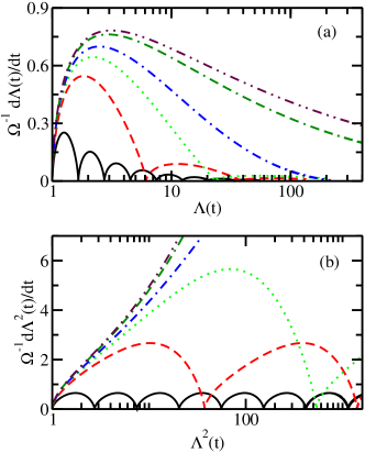
Figure 1: (Color online) Phase space trajectories that characterize the dynamics of the $N$-body system with scale invariant two-body interactions. The lines show the quantity $d\Lambda^{n}(t)/dt$ as a function of $\Lambda^{n}(t)$ for (a) $n=1$ and (b) $n=2$ for various $\lambda$. The solid, dashed, dotted, dash-dotted, dash-dash-dotted, and dot-dot-dashed lines correspond to $\lambda=0.1,1,2,3,5,$ and $6$, respectively.

This phase space representation illustrates that the cloud size increases continuously with increasing time. The expansion speed is greater or equal to zero for all $t$. For $\lambda<4$ [solid, dashed, dotted, and dash-dotted lines in Fig. 1(a)], the phase space trajectories for fixed $\lambda$ resemble those of a “bouncing ball”. The value of $\lambda$, assuming $\lambda<4$, does not affect the overall shape of the trajectory; it merely changes the spacing between and amplitude of the “bounces” (both the spacing and amplitude decrease with decreasing $\lambda$). For $\lambda>4$ [dash-dash-dotted and dot-dot-dashed lines in Fig. 1(a)], the phase space trajectories show a finite positive expansion speed for all $t>t_{0}$. In these cases, the expansion speed first increases, then reaches a maximum, and eventually decreases monotonically for all later times. In the limit $\lambda\to\infty$, i.e., in the limit of the sudden removal of the trap, the expansion speed increases to a maximum that is set by the initial energy of the systems and then remains constant after that. Figure 1(b) shows $d\Lambda^{2}(t)/dt$ as a function of $\Lambda^{2}(t)$ for various $\lambda$. These phase space trajectories characterize, according to Eq. (8), the time dynamics of the expectation value $\langle R^{2}(t)\rangle$. Qualitatively, Figs. 1(a) and 1(b) display the same characteristics.

To prepare for the discussion presented in the next section, it is instructive to explicitly write down, as was done in Ref. Deng et al. (2016), the differential equation for the expectation value $\langle R^{2}(t)\rangle$ of the square of the hyperradius,

$$\frac{d^{3}}{dt^{3}}\langle R^{2}(t)\rangle+\frac{4}{\lambda t^{2}}\frac{d}{dt}\langle R^{2}(t)\rangle-\frac{4}{\lambda t^{3}}\langle R^{2}(t)\rangle=0.$$ (11)

This equation can be derived by applying Heisenberg’s equation of motion to the $N$-particle Schrödinger equation and taking advantage of the fact that the two-body interactions do not define a meaningful length scale Deng et al. (2016). The next section considers how the differential equation for $\langle R^{2}(t)\rangle$, Eq. (11), is modified if the two-body interactions define a length scale.

II.3 Interactions with finite $g$

As already aluded to, the hyperradial and hyperangular degrees do, in general, not decouple if the interaction strength $g$ of the two-body interactions is finite, making it challenging to tackle the full $N$-body dynamics. To gain insight into the dynamics for finite $g$, we consider the simplest possible scenario, namely two interacting particles in one spatial dimension. In this case, the wave packet dynamics can be determined numerically utilizing the techniques introduced in Ref. Gharashi and Blume (2015). Moreover, analytical results for limiting cases can be used to interpret the numerical results.

For the two-particle system, the square of the hyperradius can be rewritten in terms of the relative coordinate $z$ and the center of coordinate $Z_{\rm{CM}}$, $R^{2}=z^{2}/4+(Z_{\rm{CM}})^{2}$ with $z=z_{1}-z_{2}$ and $Z_{\rm{CM}}=(z_{1}+z_{2})/2$ (from now on we use $z_{j}$ instead of $\mathbf{r}_{j}$ to emphasize the one-dimensional nature of the system under study). For the time variation defined in Eq. (7), the relative and center of mass degrees of freedom decouple, i.e., the full wave packet $\Psi(z_{1},z_{2},t)$ can be written as a product of the relative part $\psi(z,t)$ and the center of mass part $\Psi_{\rm{CM}}(Z_{\rm{CM}},t)$, $\Psi(z_{1},z_{2},t)=\psi(z,t)\Psi_{\rm{CM}}(Z_{\rm{CM}},t)$. Correspondingly, $\langle R^{2}(t)\rangle$ can be written as $\langle z^{2}(t)\rangle/4+\langle(Z_{\rm{CM}}(t))^{2}\rangle$. This implies that the time evolution of the relative and center of mass parts can be treated separately. This also means that the two-body system considered does not allow us to study the coupling between the hyperradial and hyperangular degrees of freedom. Nevertheless, it does allow us to investigate how the finite interaction strength $g$ enters into the dynamics of $\langle z^{2}(t)\rangle$.

The differential equation for the center of mass part $\langle(Z_{\rm{CM}}(t))^{2}\rangle$ is given by Eq. (11) with $R$ replaced by $Z_{\rm{CM}}$. Hence, the time evolution of $\langle(Z_{\rm{CM}}(t))^{2}\rangle$ is the same as that for a single (non-interacting) particle of mass $2m$. The differential equation for the relative part $\langle z^{2}(t)\rangle$ reads

$$\frac{d^{3}}{dt^{3}}\langle z^{2}(t)\rangle+\frac{4}{\lambda t^{2}}\frac{d}{dt}\langle z^{2}(t)\rangle-\frac{4}{\lambda t^{3}}\langle z^{2}(t)\rangle=-\frac{4\hbar^{2}}{m^{3}g}\frac{dC(t)}{dt},$$ (12)

where the Tan contact $C(t)$ is defined through Barth and Zwerger (2011)

$$C(t)=4\hbar^{2}\left[\left|\frac{d\psi(z,t)}{dz}\right|^{2}\right]_{z\to 0}.$$ (13)

Noticing that the left hand sides of Eqs. (11) and (12) have the same functional forms, we conclude that the finiteness of the interaction strength $g$ enters into the differential equation for $\langle z^{2}(t)\rangle$ via the time variation of the Tan contact. In fact, the right hand side of Eq. (12) vanishes for $g=0$ (in this case, the contact vanishes) and $|g|=\infty$ (in this case, $1/|g|$ vanishes) and Eq. (12) reduces to Eq. (11) in these cases. Equation (12) was first introduced for the general $N$ case in Refs. Qi (April 13, 2016); Shi (April 16, 2016).

To obtain a sense of how the contact $C(t)$ changes with time, we imagine that the system changes adiabatically, i.e., we determine the contact $C^{\rm{adia}}$ for the two-particle system with coupling constant $g$ in a static harmonic trap with angular frequency $\bar{\omega}$ and corresponding harmonic oscillator length $\bar{a}$. Using the expressions for the eigenenergies and eigenstates from Ref. Busch et al. (1998), the adiabatic contact for the two-body system can be calculated readily for any $g$. In preparation for the discussion in Sec. III, we consider selected limiting cases. For the eigenstates with relative energy $E_{\rm{rel}}$ around $\hbar\bar{\omega}/2$ and $3\hbar\bar{\omega}/2$, we find, respectively,

$$\frac{C_{\rm{E}_{\rm{rel}}\approx\hbar\bar{\omega}/2}^{\rm{adia}}}{\hbar^{2}\bar{a}^{-3}}=\frac{1}{\sqrt{2\pi}}\left(\frac{g}{\hbar\bar{\omega}\bar{a}}\right)^{2}+\mathcal{O}\left(g^{3}\right)$$ (14)

and

$$\frac{C_{\rm{E}_{\rm{rel}}\approx 3\hbar\bar{\omega}/2}^{\rm{adia}}}{\hbar^{2}\bar{a}^{-3}}=2\sqrt{\frac{2}{\pi}}+c_{1}\frac{a_{\text{1D}}}{\bar{a}}+c_{2}\left(\frac{a_{\text{1D}}}{\bar{a}}\right)^{2}+\mathcal{O}\left(a_{\text{1D}}^{3}\right),$$ (15)

where $c_{1}=0.781394\dots$ and $c_{2}=-2.34671\dots$ (the analytical expressions for $c_{1}$ and $c_{2}$ are lengthy and not given here). The one-dimensional scattering length $a_{\rm{1D}}$ is inversely proportional to the one-dimensional coupling constant $g$ Olshanii (1998), $a_{\rm{1D}}=-2\hbar^{2}/(mg)$. If we assume that $g$ is small and that we start in the ground state at $t=t_{0}$ and then change the trapping frequency adiabatically, the ratio of the adiabatic contact at time $t$ and that at time $t_{0}$ is $(t_{0}/t)^{1/2}$. If, on the other hand, we assume that $g$ is large ($g$ positive) and that we start in the ground state at $t=t_{0}$ and then change the trapping frequency adiabatically, the ratio of the adiabatic contact at time $t$ and that at time $t_{0}$ is $(t_{0}/t)^{3/2}$. As mentioned earlier, we are primarily interested in the regime where the Hamiltonian is changed non-adiabatically. Thus, we expect that the time dependence of the contact is not described accurately by the adiabatic prescription. Instead, we expect—taking into account that $\langle z^{2}(t)\rangle$ displays log-periodic oscillations “on top” of an overall growth in the $g=0$ and $=\infty$ limits—that the time variation of the contact for systems with finite $g$ will oscillate around the adiabatic value.

It is also interesting to consider the strongly-attractive limit ($|g|\gg\hbar\bar{\omega}\bar{a}$ and $g<0$), in which the two particles form a tightly bound dimer of size $a_{\text{1D}}$ ($a_{\text{1D}}\ll\bar{a}$). In this case, the relative wave function approaches that of two particles in free space with contact $C_{\rm{dimer}}^{\rm{free-space}}$,

$$C_{\rm{dimer}}^{\rm{free-space}}=\frac{4\hbar^{2}}{a_{\text{1D}}^{3}}.$$ (16)

Since the contact $C_{\rm{dimer}}^{\rm{free-space}}$ is independent of the harmonic oscillator length $\bar{a}$, we expect that the time-dependence of the trapping potential for $t>t_{0}$ has little impact on the initial state, provided $a_{\text{1D}}\ll\sqrt{\hbar/(m\Omega)}$. This is essentially saying that the trap is too weak in this limit to affect the initial state.

III Two-Particle Results

To solve the time-dependent Schrödinger equation in the relative coordinate $z$ for the Hamiltonian with time varying confining potential and finite $g$, we perform numerical calculations. We use a propagator that exactly accounts for the two-body zero-range interaction Blinder (1988); Wódkiewicz (1991); Yan and Blume (2015). In brief, the relative coordinate is discretized using an equidistant grid with grid spacing $\Delta z$. Knowing the wave packet at time $t$, the wave packet at time $t+\Delta t$ is obtained by integrating the product of the propagator and the wave packet at time $t$ over the relative coordinate. This propagation step is repeated for many time steps $\Delta t$. The accuracy of the final wave packet depends on the values of $\Delta z$ and $\Delta t$; implementation details can be found in Ref. Gharashi and Blume (2015). The errorbars (not shown) of the numerical results presented in this section are smaller than the symbol sizes or not visible on the chosen scales. Typical simulation parameters are $\Delta z=0.003a_{\text{ho}}(t_{0})$ and $\Delta t=0.04\Omega^{-1}$.

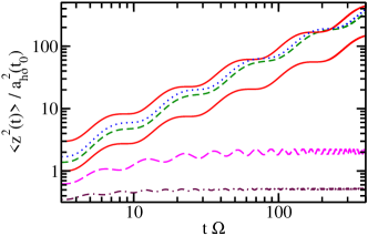
Figure 2: (Color online) Expectation value $\langle z^{2}(t)\rangle$ as a function of time for two one-dimensional particles with $\lambda=1/10$ and various interaction strengths $g$. The time evolution starts at $t\Omega=t_{0}\Omega=\sqrt{10}$. The lines from the top to the bottom at $t\Omega=\sqrt{10}$ correspond to $g/[E_{\rm{ho}}(t_{0})a_{\rm{ho}}(t_{0})]=\infty,2,1,0,-1$, and $-2$.

Figure 2 shows the expectation value $\langle z^{2}(t)\rangle$ as a function of time for various $g$ on a log-log scale. In all cases, the initial state at $t=t_{0}$ corresponds to the lowest energy eigenstate of the time-independent $t<t_{0}$ Hamiltonian. As a reference, the two solid lines show $\langle z^{2}(t)\rangle$ for the systems with scale-invariant interactions, $|g|=\infty$ (upper solid curve) and $g=0$ (lower solid curve). As discussed in Sec. II.2, the two solid curves would collapse to a single curve if the two $\langle z^{2}(t)\rangle$ were scaled by their corresponding initial $\langle z^{2}(t_{0})\rangle$. In the representation chosen in Fig. 2, the solid lines are offset from each other but exhibit the same oscillation amplitude and period. The dotted and short-dashed lines show the expectation value $\langle z^{2}(t)\rangle$ for repulsively-interacting systems with $g/[E_{\rm{ho}}(t_{0})a_{\rm{ho}}(t_{0})]=2$ and 1, respectively. For these two finite $g$ cases, the amplitude and oscillation period “dephase” over time; this dephasing is due to the finite length scale defined by the interactions. Ignoring the oscillations, $\langle z^{2}(t)\rangle$ increases faster for finite $g$ than for $g=0$. Using a hand waving argument, this can be understood by noticing that $g/[E_{\rm{ho}}(t)a_{\rm{ho}}(t)]$ increases with increasing time due to the time-dependence of the trapping frequency. At large $t$, the interactions thus effectively approach the strongly-interacting limit, explaining why the expectation value $\langle z^{2}(t)\rangle$ for finite $g$ is closer to that for $1/g=0$ than that for $g=0$; a more quantitative discussion is presented below.

The long-dashed and dash-dotted lines in Fig. 2 show $\langle z^{2}(t)\rangle$ for negative interaction strengths, i.e., for $g/[E_{\rm{ho}}(t_{0})a_{\rm{ho}}(t_{0})]=-1$ and $-2$, respectively. For these $g$, $\langle z^{2}(t)\rangle$ first increases notably with increasing $t$ and then plateaus. This can be intuitively understood by realizing that the wave packet initially, oscillations aside, expands together with the trap. At later times, however, $a_{\text{ho}}(t)$ is much larger than the size of the wave packet, and the dynamics is approximately independent of the time dependence of the trap, implying that $\langle z^{2}(t)\rangle$ approaches $a_{\text{1D}}^{2}/2$, i.e., the expectation value of $z^{2}$ for a dimer with one-dimensional scattering length $a_{\text{1D}}$ in free space. Indeed, this is what we observe in Fig. 2: The long-dashed and dash-dotted lines approach $2a_{\text{ho}}^{2}(t_{0})$ and $a_{\text{ho}}^{2}(t_{0})/2$, respectively, at large $t$. We find that the small oscillations exhibited by $\langle z^{2}(t)\rangle$ occur on a time scale that is, roughly, set by the two-body binding energy.

As discussed in Sec. II.3, the length scale introduced by the two-body interaction manifests itself in the differential equation for $\langle z^{2}(t)\rangle$ via the time derivative $dC(t)/dt$ of the contact [see Eq. (11)]. To analyze the role of this “new” term, thick lines in Fig. 3(a) show the contact $C(t)$, normalized by its initial value $C(t_{0})$, for $\lambda=1/10$ and various $g$. For finite $g$, $C(t)$ displays oscillations on top of an overall decay. The overall decay is well described by the adiabatic contact $C^{\text{adia}}(t)$, which is shown by the thin lines for each $g$ considered. As already discussed in Sec. II.3, the thin lines for the strongly-repulsive systems fall off approximately as $(t_{0}/t)^{3/2}$ for all $t$ (the approximation becomes better for larger $t$) while the thin lines for the weakly-repulsive systems transition from an initial $(t_{0}/t)^{1/2}$ fall-off to a $(t_{0}/t)^{3/2}$ fall-off for large $t$. The non-trivial time-dependence of $C(t)$ is responsible for the “dephasing” discussed in the context of Fig. 2.

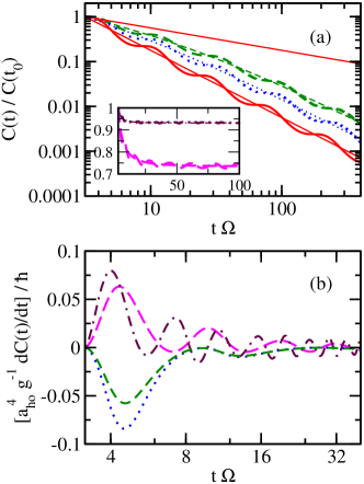
Figure 3: (Color online) Properties of the contact as a function of time for two one-dimensional particles with $\lambda=1/10$ and various interaction strengths $g$. (a) The thick lines from top to bottom show the normalized contact $C(t)/C(t_{0})$ for $g/[E_{\rm{ho}}(t_{0})a_{\rm{ho}}(t_{0})]=1$ (dashed line), $2$ (dotted line), and $\infty$ (solid line), respectively. The thin lines show the corresponding adiabatic contact $C^{\text{adia}}(t)/C(t_{0})$ using the same linestyles. The thin solid line at the top shows the limiting behavior $\sqrt{t_{0}/t}$ (see text for details). The inset shows the same quantities but for $g/[E_{\rm{ho}}(t_{0})a_{\rm{ho}}(t_{0})]=-1$ (dashed lines; upper set of curves) and $g/[E_{\rm{ho}}(t_{0})a_{\rm{ho}}(t_{0})]=-2$ (dash-dotted lines; lower set of curves). Note that the inset uses linear horizontal and vertical scales while the main figure uses logarithmic horizontal and vertical scales. (b) Dotted, short-dashed, long-dashed, and dash-dotted lines show the quantity $g^{-1}dC(t)/dt$ for $g/[E_{\rm{ho}}(t_{0})a_{\rm{ho}}(t_{0})]=2$, $1$, $-1$, and $-2$, respectively.

To see this more clearly, Fig. 3(b) shows the quantity $g^{-1}dC(t)/dt$, i.e., the right hand side of Eq. (12), for various finite $g$. While this quantity vanishes for $g=0$ and $g=\infty$, it exhibits oscillations on top of an overall decrease with increasing $t$ for finite $g$. Our analysis shows that the absolute value of each of the three terms on the left hand side of equation Eq. (12) is, for the first few oscillations, of the same order of magnitude as the absolute value of the right hand side of that equation. As time increases, the magnitude of the right hand side of Eq. (12), however, decreases faster than that of the other three terms. For positive $g$, we find that the relative importance of the right hand side decreases faster for larger $g$. This can, again, be intuitively understood by realizing that $|g|/[E_{\text{ho}}(t)a_{\text{ho}}(t)]$ increases with increasing time.

To analyze the time dependence of $\langle z^{2}(t)\rangle$ further, we think of the dynamics displayed in Fig. 2 for finite $g$ as “close to periodic” and devise empirical measures to quantify the deviations from the “truly periodic” dynamics encountered for $g=0$ and $1/g=0$. To this end, we calculate $d\langle z^{2}(t)\rangle/dt$. While $d\langle z^{2}(t)\rangle/dt$ is zero at the beginning and end of each cycle for $g=0$ or $1/g=0$ (see Fig. 1), it does not go to zero for finite $g$. For positive $g$, we thus define cycles by looking at consecutive local minima of $d\langle z^{2}(t)\rangle/dt$ and by denoting the time at which the $j$th cycle starts by $t_{\rm{in}}^{(j)}$ and the time at which the $j$th cycle ends by $t_{\rm{fi}}^{(j)}$ (the cycle enumeration starts with $j=1$). We define

$$c^{(j)}=\frac{d\langle z^{2}(t)\rangle}{dt}\Big{|}_{t=t_{\rm{fi}}^{(j)}}$$ (17)

as well as the scaling factors $\tau^{(j)}$ and $\zeta^{(j)}$,

$$\tau^{(j)}={t_{\rm{fi}}^{(j)}}/{t_{\rm{in}}^{(j)}},$$ (18)

and

$$\zeta^{(j)}=\frac{\langle z^{2}(t_{\rm{fi}}^{(j)})\rangle}{\langle z^{2}(t_{\rm{in}}^{(j)})\rangle}.$$ (19)

For $g=0$ and $|g|=\infty$, these scaling factors are independent of $j$ and given by $\tau=\zeta=\exp(2\pi/s_{0})$.

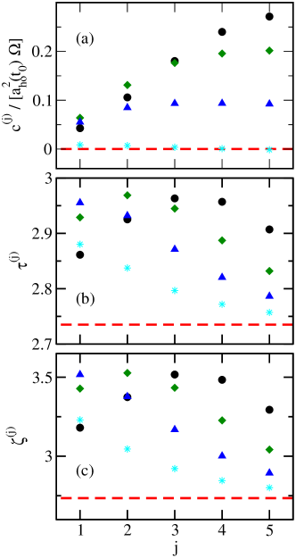
Figure 4: (Color online) Characterization of the expansion dynamics as a function of the cycle number $j$ for two-body systems with $\lambda=1/10$ and positive $g$. The symbols in panels (a), (b), and (c) show $c^{(j)}$ [Eq. (17)], $\tau^{(j)}$ [Eq. (18)], and $\zeta^{(j)}$ [Eq. (19)], respectively. The circles, diamonds, triangles, and stars correspond to $g/[E_{\rm{ho}}(t_{0})a_{\rm{ho}}(t_{0})]=1/2,1,2$, and $5$, respectively. The horizontal dashed lines show the corresponding values for the case where the two-body interaction does not define a meaningful length scale ($g=0$ or $|g|=\infty$); in this case, we have $\tau=\zeta=\exp(2\pi/s_{0})\approx 2.734955$.

Circles, diamonds, triangles, and stars in Fig. 4 show our numerical results for Eqs. (17)-(19) for $g/[E_{\rm{ho}}(t_{0})a_{\rm{ho}}(t_{0})]=1/2,1,2$, and $5$, respectively. For comparison, the dashed lines show the corresponding values for the scale-invariant systems. For the two largest $g$ considered (stars and triangles), $\tau^{(j)}$ and $\zeta^{(j)}$ decrease monotonically with increasing $j$. Figures 4(b) and 4(c) suggest that the large $j$ limit is given by the horizontal dashed lines, i.e., that the scale factors for finite $g$ at large $t$ approach the scale factor of the scale-invariant systems. For smaller $g$ (diamonds and circles), the scale factors first increase, then reach a maximum, and finally decrease. Although our numerics does not allow us to go beyond $j=5$, Figs. 4(b) and 4(c) suggest that the scale factors for systems with these smaller $g$ values also approach the scale-invariant value in the large $j$ limit. The quantity $c^{(j)}$ [see Fig. 4(a)], in contrast, does not approach the value of the scale invariant systems but instead approaches a finite constant for large $j$. The asymptotic, large $j$ value is reached faster for large $g$ than for small $g$.

We now present analytical considerations for systems with finite positive $g$ that explain the trends displayed in Fig. 4. As mentioned already several times, $g/[E_{\text{ho}}(t)a_{\text{ho}}(t)]$ increases with increasing time. Thus, we neglect the right hand side of Eq. (12) in the large $t$ limit and analyze the analytical solution, which can be found in Ref. Lewis (1968), for the differential equation assuming finite values for $\langle z^{2}(t^{\prime})\rangle$ and $[d\langle z^{2}(t)\rangle/dt]_{t=t^{\prime}}$, where $t^{\prime}\gg t_{0}$. The reason for using a finite value for $[d\langle z^{2}(t)\rangle/dt]_{t=t^{\prime}}$ is that the wave packet at $t=t^{\prime}$ is not in an eigenstate [indeed, Fig. 4(a) shows that $c^{(j)}$ is finite]. We find that the analytical solution for the initial conditions applicable to an initial non-stationary state exhibits the same log-periodic oscillation period and amplitude as the analytical solution for the initial conditions applicable to an initial stationary state. This explains why the scaling factors $\tau^{(j)}$ and $\zeta^{(j)}$ [see Figs. 4(b) and 4(c)] approach the dashed horizontal lines in the large $j$ limit. Moreover, since the analytical description is expected to become more accurate for larger $j$, $c^{(j)}$ is expected to approach a constant in the large $j$ limit.

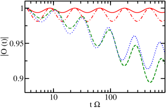
Figure 5: (Color online) Norm $|O(t)|$ of the overlap [see Eq. (20)] as a function of time for two one-dimensional particles with $\lambda=1/10$ and various interaction strengths $g$. Solid, dash-dotted, dashed, and dotted lines correspond to $g/[E_{\rm{ho}}(t_{0})a_{\rm{ho}}(t_{0})]=0$, $\infty$, $1$, and $2$, respectively.

While the discussion above shows that certain properties of the large $t$ dynamics can be predicted analytically, the full wave packet dynamics for finite $g$ may be quite intricate, i.e., the quantities $\langle z^{2}(t)\rangle$ and $d\langle z^{2}(t)\rangle/dt$ alone may not describe the full story. To corroborate this notion, we consider the time-dependent overlap $O(t)$ between the wave packet $\psi(z,t)$ and the adiabatic eigenstate $\psi^{\rm{adia}}(z,a_{\rm{ho}}(t))$ for the same $g$ and confinement with harmonic oscillator length $a_{\text{ho}}(t)$,

$$O(t)=\langle\psi(z,t)|\psi^{\rm{adia}}\left(z,a_{\rm{ho}}(t)\right)\rangle.$$ (20)

Figure 5 shows $|O(t)|$ (the absolute value is taken to eliminate arbitrary phase factors) as a function of time for various coupling strengths $g$. For $g=0$ (solid line) and $\infty$ (dash-dotted line), $|O(t)|$ is equal to 1 at the end of each cycle, reflecting the fact that the wave packet returns, provided the appropriate scaling of the $z$ coordinate is applied, to its orginal shape. Interestingly, $|O(t)|$ takes on its minimal values at the “half-cycle” times, i.e., at the times where $\langle z^{2}(t)\rangle$ coincides with the corresponding adiabatic value. For finite $g$, the norm $|O(t)|$ of the overlap displays, as for the scale-invariant interactions, oscillatory behavior. However, the oscillations are on top of an overall decrease of the overlap. This implies that the finite length scale continually introduces a dephasing, i.e., the time-dependent wave packet is increasingly less similar to the adiabatic eigenstate. Said differently, excited adiabatic states get mixed in more with increasing time $t$. Taking a slightly different view point, this means that a full description of the wave packet at the end of the empirically defined cycles requires knowledge not only of $\langle z^{2}(t)\rangle$ but of $\langle z^{n}(t)\rangle$ for all $n$.

IV Conclusion

This paper investigated the expansion dynamics of a harmonically trapped cold atom system with zero-range interactions. For $t<t_{0}$, the angular trap frequency $\omega(t)$ is equal to the constant $\Omega$ and the system is in an eigenstate. For $t>t_{0}$, a scale-invariant trap potential is realized by varying the angular frequency smoothly according to $\omega(t)=\Omega t_{0}/t$. The scale invariance can be most readily seen from Eq. (11), where $R$ and $t$ occur with the same powers in all three terms. More formally, we can look at how the Hamiltonian changes if the position coordinates are multiplied by $\alpha$. In this case, the kinetic energy term picks up an extra $\alpha^{-2}$ factor while the time-independent trapping potential picks up an extra factor of $\alpha^{2}$; thus, the system Hamiltonian possesses a scale (namely the harmonic oscillator length). Scaling the time by $\alpha^{2}$ (this follows from the fact that time is, dimensionally, $\hbar$ divided by energy and that energy scales as one over length to the power of two), the time-dependent trapping potential, which contains terms like $\omega^{2}(t)\mathbf{r}_{j}^{2}$, picks up a factor of $\alpha^{-2}$, just as the kinetic energy term; thus, the system Hamiltonian does not possess a scale, i.e., it is scale-invariant.

If the interaction strength $g$ vanishes or is infinitely large, the entire systems Hamiltonian is scale-invariant. In this case, the expansion dynamics has been investigated experimentally and theoretically in Ref. Deng et al. (2016). It was found that the cloud size follows so-called Efimovian expansion dynamics with logarithmically spaced oscillation periods and amplitudes.

The present paper investigated how the expansion dynamics changes if the interaction strength $g$ is finite. To address this question, the simplest non-trivial system consisting of two one-dimensional particles was investigated. It was found that the expansion dynamics of systems with finite and positive $g$ still exhibits oscillatory behavior. However, the oscillation period and amplitude are no longer logarithmically spaced. Instead, a dephasing that is governed by the time derivative of the contact is observed. At large times (depending on the value of $g$, this may imply large numbers of “close-to-periodic” oscillations), we found that the cloud size is again, at least approximately, governed by a unique oscillation period and amplitude. We note that the role of the contact in non-equilibrium situations was previously investigated in two-atom quantum quenches Corson and Bohn (2016), where a rapid change of the interaction strength (a quench) induced a ballistic component into the contact. In the scenario considered in the present paper, the oscillations of the contact are the result of the continuously changing trapping potential. The work done on the system for $t>t_{0}$ triggers an interplay between the harmonic oscillator parts of the Hamiltonian and the two-body interaction terms. When the cloud is extremely dilute (large times), the effective interaction strength of the one-dimensional system becomes large [$g/[E_{\text{ho}}(t)a_{\text{ho}}(t)]$ increases as $g\sqrt{t}$]. Thus, the system is, again, effectively scale-invariant at large times, implying—using the general solutions for the scale-invariant system with modified initial conditions—close-to-log-periodic expansion dynamics. While our analysis in Sec. III considered two one-dimensional particles with finite interaction strength, the results generalize to systems consisting of more particles and with other dimensionalities.

The design of time-dependent trapping potentials has played an important role over the past 60 years or so. Here, the role of finite two-body interaction strengths on the Efimovian-like expansion dynamics was investigated. In other contexts (see, e.g., Ref. Chen et al. (2010)), time-dependent trapping potentials have been used to design frictionless non-adiabatic atom cooling trajectories. It would be interesting to include atom-atom interactions in those contexts via the contact and to quantify the energy distribution among the various modes, building on the ideas put forward in Ref. Ebert et al. (2016).

V Acknowledgments

Support by the National Science Foundation (NSF) through Grant No. PHY-1415112 is gratefully acknowledged. This work used the Extreme Science and Engineering Discovery Environment (XSEDE), which is supported by NSF Grant No. OCI-1053575, and the WSU HPC.

References

- Fetter and Walecka (2003) A. L. Fetter and J. D. Walecka, Quantum Theory of Many-particle Systems, Dover Books on Physics (Dover Publications, 2003).
- Stöckmann (2006) H. J. Stöckmann, Quantum Chaos: An Introduction (Cambridge University Press, 2006).
- Nikolopoulos and Jex (2013) G. M. Nikolopoulos and I. Jex, Quantum State Transfer and Network Engineering, Quantum Science and Technology (Springer Berlin Heidelberg, 2013).
- Menchon-Enrich et al. (2016) R. Menchon-Enrich, A. Benseny, V. Ahufinger, A. D. Greentree, T. Busch, and J. Mompart, “Spatial adiabatic passage: a review of recent progress,” Reports on Progress in Physics 79, 074401 (2016).
- Polo et al. (2016) J. Polo, A. Benseny, T. Busch, V. Ahufinger, and J. Mompart, “Transport of ultracold atoms between concentric traps via spatial adiabatic passage,” New Journal of Physics 18, 015010 (2016).
- Polkovnikov et al. (2011) A. Polkovnikov, K. Sengupta, A. Silva, and M. Vengalattore, “Nonequilibrium dynamics of closed interacting quantum systems,” Rev. Mod. Phys. 83, 863–883 (2011).
- Yan et al. (2013) B. Yan, S. A. Moses, B. Gadway, J. P. Covey, K. R. A. Hazzard, A. M. Rey, D. S. Jin, and J. Ye, “Observation of dipolar spin-exchange interactions with lattice-confined polar molecules,” Nature 501, 521–525 (2013).
- Aoki et al. (2014) H. Aoki, N. Tsuji, M. Eckstein, M. Kollar, T. Oka, and Ph. Werner, “Nonequilibrium dynamical mean-field theory and its applications,” Rev. Mod. Phys. 86, 779–837 (2014).
- Makotyn et al. (2014) P. Makotyn, C. E. Klauss, D. L. Goldberger, E. A. Cornell, and D. S. Jin, “Universal dynamics of a degenerate unitary Bose gas,” Nature Physics 10, 116–119 (2014).
- Langen et al. (2015) T. Langen, S. Erne, R. Geiger, B. Rauer, T. Schweigler, M. Kuhnert, W. Rohringer, I. E. Mazets, T. Gasenzer, and J. Schmiedmayer, “Experimental observation of a generalized Gibbs ensemble,” Science 348, 207–211 (2015).
- Will et al. (2015) S. Will, D. Iyer, and M. Rigol, “Observation of coherent quench dynamics in a metallic many-body state of fermionic atoms,” Nature Communications 6, 6009 (2015).
- Cetina et al. (2016) M. Cetina, M. Jag, R. S. Lous, I. Fritsche, J. T. M. Walraven, R. Grimm, J. Levinsen, M. M. Parish, R. Schmidt, M. Knap, and E. Demler, “Ultrafast many-body interferometry of impurities coupled to a Fermi sea,” ArXiv e-prints (2016), arXiv:1604.07423 [cond-mat.quant-gas] .
- Blakie and Porto (2004) P. B. Blakie and J. V. Porto, “Adiabatic loading of bosons into optical lattices,” Phys. Rev. A 69, 013603 (2004).
- Gericke et al. (2007) T. Gericke, F. Gerbier, A. Widera, S. Fölling, O. Mandel, and I. Bloch, “Adiabatic loading of a Bose-Einstein condensate in a 3D optical lattice,” Journal of Modern Optics 54, 735–743 (2007).
- Rosi et al. (2013) S. Rosi, A. Bernard, N. Fabbri, L. Fallani, C. Fort, M. Inguscio, T. Calarco, and S. Montangero, “Fast closed-loop optimal control of ultracold atoms in an optical lattice,” Phys. Rev. A 88, 021601 (2013).
- Masuda et al. (2014) S. Masuda, K. Nakamura, and A. del Campo, “High-Fidelity Rapid Ground-State Loading of an Ultracold Gas into an Optical Lattice,” Phys. Rev. Lett. 113, 063003 (2014).
- Lode et al. (2012) A. U. J. Lode, A. I. Streltsov, K. Sakmann, O. E. Alon, and L. S. Cederbaum, “How an interacting many-body system tunnels through a potential barrier to open space,” Proceedings of the National Academy of Sciences 109, 13521–13525 (2012).
- Sykes et al. (2014) A. G. Sykes, J. P. Corson, J. P. D’Incao, A. P. Koller, C. H. Greene, A. M. Rey, K. R. A. Hazzard, and J. L. Bohn, “Quenching to unitarity: Quantum dynamics in a three-dimensional bose gas,” Phys. Rev. A 89, 021601 (2014).
- Zürn et al. (2012) G. Zürn, F. Serwane, T. Lompe, A. N. Wenz, M. G. Ries, J. E. Bohn, and S. Jochim, “Fermionization of Two Distinguishable Fermions,” Phys. Rev. Lett. 108, 075303 (2012).
- Zürn et al. (2013) G. Zürn, A. N. Wenz, S. Murmann, A. Bergschneider, T. Lompe, and S. Jochim, “Pairing in Few-Fermion Systems with Attractive Interactions,” Phys. Rev. Lett. 111, 175302 (2013).
- Gharashi and Blume (2015) S. E. Gharashi and D. Blume, “Tunneling dynamics of two interacting one-dimensional particles,” Phys. Rev. A 92, 033629 (2015).
- Ebert et al. (2016) M. Ebert, A. Volosniev, and H.-W. Hammer, “Two cold atoms in a time-dependent harmonic trap in one dimension,” Annalen der Physik (2016), 10.1002/andp.201500365.
- Corson and Bohn (2016) John P. Corson and John L. Bohn, “Ballistic quench-induced correlation waves in ultracold gases,” Phys. Rev. A 94, 023604 (2016).
- Deng et al. (2016) Sh. Deng, Z.-Y. Shi, P. Diao, Q. Yu, H. Zhai, R. Qi, and H. Wu, “Observation of the Efimovian expansion in scale-invariant Fermi gases,” Science 353, 371–374 (2016).
- Efimov (1970) V. Efimov, “Energy levels arising from resonant two-body forces in a three-body system,” Physics Letters B 33, 563 – 564 (1970).
- Braaten and Hammer (2006) E. Braaten and H.-W. Hammer, “Universality in few-body systems with large scattering length,” Physics Reports 428, 259–390 (2006).
- Chin et al. (2010) C. Chin, R. Grimm, P. Julienne, and E. Tiesinga, “Feshbach resonances in ultracold gases,” Reviews of Modern Physics 82, 1225–1286 (2010).
- Giorgini et al. (2008) S. Giorgini, L. P. Pitaevskii, and S. Stringari, “Theory of ultracold atomic Fermi gases,” Reviews of Modern Physics 80, 1215–1274 (2008).
- Zwerger (2011) W. Zwerger, ed., The BCS-BEC Crossover and the Unitary Fermi Gas, Lecture Notes in Physics (Springer, Berlin, 2011).
- Jonsell et al. (2002) S. Jonsell, H. Heiselberg, and C. J. Pethick, “Universal behavior of the energy of trapped few-boson systems with large scattering length,” Phys. Rev. Lett. 89, 250401 (2002).
- Werner and Castin (2006) F. Werner and Y. Castin, “Unitary gas in an isotropic harmonic trap: Symmetry properties and applications,” Phys. Rev. A 74, 053604 (2006).
- footnote7- (1) An example is the two-component Fermi gas with vanishing intraspecies interaction strength and infinitely large interspecies interaction strength.
- von Stecher et al. (2008) J. von Stecher, C. H. Greene, and D. Blume, “Energetics and structural properties of trapped two-component Fermi gases,” Phys. Rev. A 77, 043619 (2008).
- von Stecher and Greene (2009) J. von Stecher and C. H. Greene, “Correlated gaussian hyperspherical method for few-body systems,” Phys. Rev. A 80, 022504 (2009).
- Lewis (1967) H. R. Lewis, “Classical and quantum systems with time-dependent harmonic-oscillator-type hamiltonians,” Phys. Rev. Lett. 18, 510–512 (1967).
- Lewis (1968) H. R. Lewis, Jr., “Class of Exact Invariants for Classical and Quantum Time-Dependent Harmonic Oscillators,” Journal of Mathematical Physics 9, 1976–1986 (1968).
- Lewis and Riesenfeld (1969) H. R. Lewis, Jr. and W. B. Riesenfeld, “An Exact Quantum Theory of the Time-Dependent Harmonic Oscillator and of a Charged Particle in a Time-Dependent Electromagnetic Field,” Journal of Mathematical Physics 10, 1458–1473 (1969).
- Popov and Perelomov (1969a) V. S. Popov and A. M. Perelomov, “Parametric Excitation of a Quantum Oscillator,” Soviet Journal of Experimental and Theoretical Physics 29, 738 (1969a).
- Popov and Perelomov (1969b) V. S. Popov and A. M. Perelomov, “Parametric Excitation of a Quantum Oscillator. II,” Soviet Journal of Experimental and Theoretical Physics 30, 910 (1969b).
- Camiz et al. (1971) P. Camiz, A. Gerardi, C. Marchioro, E. Presutti, and E. Scacciatelli, “Exact Solution of a Time-Dependent Quantal Harmonic Oscillator with a Singular Perturbation,” Journal of Mathematical Physics 12, 2040–2043 (1971).
- Castin (2004) Y. Castin, “Exact scaling transform for a unitary quantum gas in a time dependent harmonic potential,” Comptes Rendus Physique 5, 407–410 (2004).
- Moroz (2012) S. Moroz, “Scale-invariant Fermi gas in a time-dependent harmonic potential,” Phys. Rev. A 86, 011601 (2012).
- Barth and Zwerger (2011) M. Barth and W. Zwerger, “Tan relations in one dimension,” Annals of Physics 326, 2544 – 2565 (2011).
- Qi (April 13, 2016) R. Qi, “The Efimovian expansion in scale invariant quantum gases,” (The First Beijing-Tokyo Workshop on Ultracold Atomic Gases, Beijing, China, April 13, 2016).
- Shi (April 16, 2016) Z.-Y. Shi, “Efimovian expansion in scale invariant quantum gases,” (International Conference on Few-body Physics in Cold Atomic Gases, Beijing, China, April 16, 2016) ”http://theory.iphy.ac.cn/FBPCAG2016/pdf/Zheyu.pdf”.
- Busch et al. (1998) T. Busch, B.-G. Englert, K. Rza̧żewski, and M. Wilkens, “Two Cold Atoms in a Harmonic Trap,” Foundations of Physics 28, 549–559 (1998).
- Olshanii (1998) M. Olshanii, “Atomic Scattering in the Presence of an External Confinement and a Gas of Impenetrable Bosons,” Phys. Rev. Lett. 81, 938–941 (1998).
- Blinder (1988) S. M. Blinder, “Green’s function and propagator for the one-dimensional -function potential,” Phys. Rev. A 37, 973–976 (1988).
- Wódkiewicz (1991) K. Wódkiewicz, “Fermi pseudopotential in arbitrary dimensions,” Phys. Rev. A 43, 68–76 (1991).
- Yan and Blume (2015) Y. Yan and D. Blume, “Incorporating exact two-body propagators for zero-range interactions into -body Monte Carlo simulations,” Phys. Rev. A 91, 043607 (2015).
- Chen et al. (2010) X. Chen, A. Ruschhaupt, S. Schmidt, A. del Campo, D. Guéry-Odelin, and J. G. Muga, “Fast optimal frictionless atom cooling in harmonic traps: Shortcut to adiabaticity,” Phys. Rev. Lett. 104, 063002 (2010).