Measurement of single $\uppi^{0}$ production by coherent neutral-current $\nu$ Fe interactions in the MINOS Near Detector

Abstract

Forward single $\uppi^{0}$ production by coherent neutral-current interactions, $\nu\,\mathcal{A}\to\nu\,\mathcal{A}\,\uppi^{0}$, is investigated using a 2.8$\times 10^{20}$ protons-on-target exposure of the MINOS Near Detector. For single-shower topologies, the event distribution in production angle exhibits a clear excess above the estimated background at very forward angles for visible energy in the range 1-8 GeV. Cross sections are obtained for the detector medium comprised of 80% iron and 20% carbon nuclei with $\langle\mathcal{A}\rangle=48$, the highest-$\langle\mathcal{A}\rangle$ target used to date in the study of this coherent reaction. The total cross section for coherent neutral-current single-$\uppi^{0}$ production initiated by the $\nu_{\mu}$ flux of the NuMI low-energy beam with mean (mode) $E_{\nu}$ of 4.9 GeV (3.0 GeV), is $77.6\pm 5.0\,(\text{stat})^{+15.0}_{-16.8}\,(\text{syst})\times 10^{-40}\,\text{cm}^{2}~{}\text{per nucleus}$. The results are in good agreement with predictions of the Berger-Sehgal model.

I Introduction

I.1 $\nu$ NC($\uppi^{0}$) coherent scattering

It is well established that single pions can be produced when a neutrino or antineutrino scatters coherently from a target nucleus ref:Paschos-Schalla-2009 . These interactions can proceed either as neutral-current (NC) or charged-current (CC) processes in which the pion electric charge coincides with that of the Z⁰ or W^± vector boson emitted by the leptonic current. Recent investigations, both experimental ref:K2K_2 ; ref:SciBooNE-CC ; ref:NOMAD ; ref:MiniBooNE ; ref:SciBooNE and theoretical ref:Paschos ; ref:RS_paper_2 ; ref:BS ; ref:Hernandez-2009 ; ref:Singh-2006 ; ref:Alvarez-Ruso-2009 ; ref:Martini-2009 ; ref:Amaro-2009 ; ref:Nakamura-2010 ; ref:Hernandez-2010 , have devoted attention to neutrino-induced NC coherent production of single $\uppi^{0}$ mesons:

$$\nu(\bar{\nu})+\mathcal{A}\rightarrow\nu(\bar{\nu})+\mathcal{A}+\uppi^{0}\bf{.}$$ (1)

Reaction (1) is of theoretical interest as a process dominated by the divergence of the isovector axial-vector neutral current and therefore amenable to calculation using the Partially Conserved Axial-Vector Current (PCAC) hypothesis and Adler’s theorem ref:Adler-theorem . The phenomenological model of Rein and Sehgal ref:RS_paper_1 invokes Adler’s theorem to express the coherent cross section in terms of the $\uppi$-nucleon scattering cross section. The original Rein-Sehgal model characterized coherent scattering at incident energies $E_{\nu}>3$ GeV, and served as a framework for development of other PCAC-based models of coherent $\uppi^{0}$ production ref:RS_paper_2 ; ref:BS ; ref:Paschos ; ref:Hernandez-2009 . In particular, the Berger-Sehgal model ref:BS used in the present work improves upon Rein-Sehgal by using $\uppi$-carbon scattering data rather than $\uppi$-nucleon data as the basis for extrapolation.

An alternative class of models, appropriate for sub-GeV to few-GeV neutrino scattering, has also received considerable attention ref:Singh-2006 ; ref:Alvarez-Ruso-2009 ; ref:Martini-2009 ; ref:Amaro-2009 ; ref:Nakamura-2010 ; ref:Hernandez-2010 . In these “dynamical models” the amplitudes for various neutrino-nucleon reactions yielding the single pion final state are added coherently over the nucleus. Within the past decade the theoretical descriptions of coherent NC $\uppi^{0}$ production for $E_{\nu}$ below a few GeV have achieved a level of detail previously unavailable ref:Boyd-2009 .

Experimental investigations of coherent NC($\uppi^{0}$) production to date have been limited to scattering on targets with an average nucleon number, $\langle\mathcal{A}\rangle$, in the range $\langle\mathcal{A}\rangle\leq 30$ (see Table  1). In the study reported here, the cross section for Reaction (1) is measured using a high statistics sample of neutrino interactions recorded by the MINOS Near Detector ref:NIM ; ref:CCinclusive . The Near Detector consists of iron plates interleaved with plastic scintillator, yielding an average nucleon number of 48. Thus the MINOS measurement probes the coherent Reaction (1) using a target with $\langle\mathcal{A}\rangle$ distinctly higher than utilized previously, as detailed in Sec. I.3.

I.2 Reaction phenomenology

In coherent scattering no quantum numbers are transferred to the target nucleus, and the square of the four-momentum transfer to the nucleus, $|t|=|(q-p_{\pi})^{2}|$, is very small. Figure 1 depicts the amplitude proposed by Rein and Sehgal to describe coherent NC($\uppi^{0}$) production in the limit $Q^{2}\equiv-q^{2}=-(p-p^{\prime})^{2}\rightarrow 0$ where both the Conserved Vector Current (CVC) and the PCAC hypotheses apply. The differential cross section away from $Q^{2}$ = 0 can be estimated using the hadron dominance model ref:HDM ; ref:K-M . In the Rein-Sehgal and Berger-Sehgal models this is accomplished using a dipole term of the form $(M_{A}^{2}/(M_{A}^{2}+Q^{2}))^{2}$.

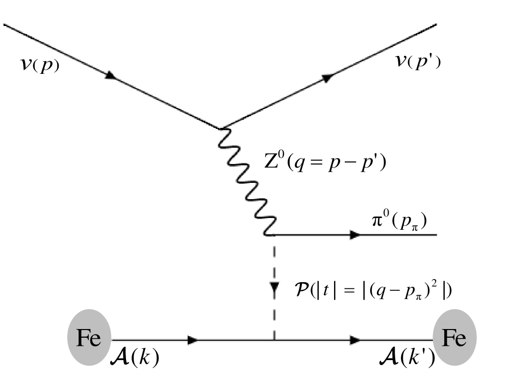
Figure 1: Mechanism for neutrino-nucleus NC($\uppi^{0}$) coherent scattering. The Z⁰ boson initiates virtual $\uppi^{0}$ elastic scattering with exchange of a pomeron-like quantum ($\mathcal{P}$) which transfers four-momentum squared $|t|$ to the nucleus.

The four-momentum of the final state lepton is not measurable in NC reactions and so $|t|$ cannot be ascertained. However, the $Q^{2}$ dependence can be related to the observable $\eta_{\small{\uppi}}$ which is a measure of the momentum transverse to the incident beam ref:MiniBooNE ; ref:Amaro-2009 :

$$\mbox{$\eta_{\small{\uppi}}$}=E_{vis}\times(1-\cos\theta_{shw})\bf{.}$$ (2)

Here, $E_{vis}$ is the visible energy of the gamma conversions resulting from $\uppi^{0}$ decay and $\theta_{shw}$ is the angle of the electromagnetic shower with respect to the beam direction. Distributions of $\eta_{\small{\uppi}}$ for coherent NC($\uppi^{0}$) events exhibit a distinctive peak at low values (see Sec. IV). However it is $\cos\theta_{shw}$ and $E_{vis}$, rather than $\eta_{\small{\uppi}}$, that serve as the basic observables for the MINOS measurement. The analysis uses event distributions in these two variables to construct its background model and to extract the signal.

I.3 Previous measurements

The first evidence for coherent neutrino-nucleus scattering was obtained by the Aachen-Padova collaboration using spark chambers constructed of aluminum plates ref:AachenPadova . Other coherent scattering measurements were carried out during the 1980s using neutrino beams with different spectra and different target nuclei ref:Gargamelle ; ref:SKAT ; ref:CHARM ; ref:15BC . More recently, the NOMAD and SciBooNE experiments have measured the coherent NC($\uppi^{0}$) cross section on carbon ref:NOMAD ; ref:SciBooNE . The MiniBooNE experiment has determined the ratio, $f_{coh}$, of NC($\uppi^{0}$) coherent to coherent-and-resonant production on carbon: $f_{coh}=0.195\pm 0.011$(stat)$\pm 0.025$(sys) ref:MiniBooNE . The latter measurements, together with searches for coherent CC($\uppi^{\pm}$) scattering by K2K ref:K2K_2 and SciBooNE ref:SciBooNE-CC , stimulated further theoretical work ref:Wascko-review . The coherent NC($\uppi^{0}$) cross sections for all previous experiments are summarized in Table 1.

Experiment				Cross Section per nucleus
	$<E_{\nu}>$	Target $\langle\mathcal{A}\rangle$	$E^{min}_{\uppi^{0}}$	$\upsigma$	$\upsigma$/$\upsigma_{\mathrm{R-S}}$	$\upsigma_{\mathrm{B-S}}$
				$\nu$($\bar{\nu}$)	$\nu$($\bar{\nu}$)
	[GeV]	[u]	[GeV]	$10^{-40}{\rm cm}^{2}$	-	$10^{-40}{\rm cm}^{2}$
Aachen-	2	Aluminum	0.18	29$\pm$10	-	31
Padova ref:AachenPadova		27		(25$\pm$7)	-
Gargamelle	3.5	Freon	0.2	31$\pm$20	-	45
ref:Gargamelle		CF3Br - 30		(45$\pm$24)	-
CHARM	31	Marble	6.0	96$\pm$42	-	82
ref:CHARM	24	CaCO3 - 20		(79$\pm$26)	-
SKAT	7	Freon	0.2	52$\pm$19	-	62
ref:SKAT		CF3Br - 30			-
15’ BC	20	Neon	2.0	-	0.98$\pm$0.24	71
ref:15BC		NeH2 - 20		-
NOMAD	24.8	Carbon+	0.5	72.6$\pm$10.6	-	53
ref:NOMAD		12.8			-
SciBooNE	0.8	Polystyrene	0.0	-	0.96$\pm$0.20	9
ref:SciBooNE		C8H8 - 12		-

Table 1: Previous cross section measurements for Reaction (1). Cross sections as directly reported are displayed in column 5; values reported as ratios to Rein-Sehgal $\upsigma_{\mathrm{R-S}}$ are listed in column 6. Cross sections obtained using $\bar{\nu}$ beams are given in parentheses. Column 7 lists corresponding predictions ($\upsigma_{\mathrm{B-S}}$) from the Berger-Sehgal model.

Recently, measurements of charged-current coherent scattering cross sections on carbon and on argon, $\mbox{$\nu_{\mu}$}\,(\bar{\nu}_{\mu})+\mathcal{A}\rightarrow\mu^{\mp}+\mathcal{A}+\uppi^{\pm}$, have been reported by MINER$\nu$A ref:CC-Coh-Minerva and by ArgoNeuT ref:CC-Coh-Argon respectively. The neutrino fluxes for these measurements, obtained with operation of the NuMI beam in low energy mode, are similar to the neutrino flux used for the present study. For neutrino-nucleus scattering at $E_{\nu}>$ 3 GeV, the PCAC models predict the final-state pion kinematics for coherent NC($\uppi^{0}$) scattering to be very similar to the kinematics observed in coherent CC($\uppi^{\pm}$) scattering. Consequently the distributions reported for the full range of $E_{\pi}$ from CC($\uppi^{\pm}$) coherent scattering ref:CC-Coh-Minerva provide guidance for estimation of the coherently-produced $\uppi^{0}$ rate below the MINOS threshold for electromagnetic (EM) shower detection.

II Analysis Overview

Measurement of the NC($\uppi^{0}$) coherent scattering cross section requires that this rare reaction, predicted to constitute about $0.2$% of all neutrino interactions in the exposure, be detected amidst a copious background of neutrino reactions having topologies that are dominated by an EM shower. The background is mostly composed of NC reactions wherein an incoherently produced, energetic $\uppi^{0}$ dominates the final-state. Backgrounds also arise from energetic $\uppi^{0}$ initiated by CC $\nu_{\mu}$ interactions with large fractional energy transfer to the hadronic system, and from quasielastic-like CC $\nu_{e}$ interactions.

This analysis uses a reference Monte Carlo (MC) event sample simulated using the NEUGEN3 event generator ref:neugen3 and other codes of the standard MINOS software framework ref:minos-QE . The reference MC sample includes NC($\uppi^{0}$) coherent scattering generated according to the Berger-Sehgal model.

Candidate events are isolated by requiring containment within the fiducial volume, absence of charged particle tracks, and visible energy sufficient to reconstruct an EM shower with $E_{vis}>$ 1.0 GeV. Further background reduction is achieved by distinguishing electromagnetic from hadronic-shower behavior using a multivariate analysis classification algorithm known as Support Vector Machines ref:Statistical-Learning ; ref:LibSVM .

Subsamples of the selected MC sample are organized and handled as binned event distributions that are functions of the kinematic variables $\cos\theta_{shw}$ and $E_{vis}$. An event distribution of this kind constitutes a “template” over the plane of $\cos\theta_{shw}$-versus-$E_{vis}$ (discussed in Sec. VI). Each of the different background reaction categories is embodied by its template distribution. These subsample templates extend over the signal region (defined by a relatively high signal-to-background ratio) and over the sidebands (kinematic regions adjacent or close to the signal region with low predicted signal content).

The background templates are constrained by fitting to data events in the sidebands. The fit adjusts the normalizations and shapes of the background templates using normalization fit parameters plus two systematic parameters; the latter account for the effects of specific sources of uncertainty capable of generating template shape distortions. Fitting to sidebands is restricted to regions that, according to the MC, have signal purity less than $5\%$, since optimization studies showed this cut to minimize the total uncertainty propagated to the measurement. The ensemble of templates, fit to the sidebands, define a background model that also extends over the signal region of the $\cos\theta_{shw}$-vs-$E_{vis}$ plane.

The formalism used to subtract background from data in the signal region is discussed in Secs. VII and VIII. The delineation, evaluation, and method of treatment of systematic uncertainties are presented in Sec. IX. At this point the foundation is set for fitting the background model to the data sidebands. Results of this fit are given in Sec. X, and the background rate over the signal region is thereby established. The subtraction of the background from the data in the signal region yields the measured number of NC($\uppi^{0}$) coherent scattering events (Sec. XI), enabling the scattering cross sections to be determined (Sec. XII). Section XIII discusses the MINOS cross sections in the context of previously reported NC($\uppi^{0}$) coherent scattering measurements and summarizes the observational results of this work.

Data blinding protocols were used throughout the development of the analysis. Data bins for which the signal purity was predicted by the MC simulation to exceed $20\%$ were always masked. Additionally, protocols were followed that forbade data versus MC comparisons and fits involving the data sidebands until all work to establish the fit procedure was completed.

II.1 Flux-averaged cross section measurement

For coherent NC($\uppi^{0}$) events, the visible energy of the final-state $\uppi^{0}$ is only a fraction of the incident neutrino energy, $E_{\nu}$. Extraction of the reaction cross section as a function of $E_{\upnu}$ is therefore problematic. Nevertheless, a flux-averaged cross section, $\langle\upsigma\rangle$, representative of a designated $E_{\nu}$ range can be measured. Let $\mathcal{N}_{T}$ denote the number of target nuclei in the Near Detector fiducial volume. The total neutrino flux for the experiment is $\mathcal{N}_{\text{p}}\times\Phi$, where $\mathcal{N}_{\text{p}}$ is the total number of protons on target (POT) and $\Phi$ is the integral over $E_{\nu}$ of the flux spectrum per POT at the front surface of the fiducial volume, $\phi(E_{\nu})$: $\Phi=\int\phi(E_{\nu}){\text{d}}E_{\nu}$. The number of reactions after correction for detection inefficiencies, $N^{Coh}$, is given by

$$N^{Coh}=~{}\mathcal{N}_{T}\,\mathcal{N}_{\text{p}}\int\upsigma(E_{\nu})\,\phi(E_{\nu})\,{\text{d}}E_{\nu}~{},$$ (3)

so that

$$\langle\upsigma\rangle=\frac{N^{Coh}}{\mathcal{N}_{T}\,\mathcal{N}_{\text{p}}\,\Phi}~{}\bf{.}$$ (4)

The constants $\mathcal{N}_{T}$, $\mathcal{N}_{\text{p}}$, and $\Phi$ are determined by the experimental setup and running conditions. The fully corrected count of signal events, $N^{Coh}$, effectively measures the flux-averaged cross section.

III Beam, Detector, Data Exposure

III.1 Neutrino beam and Near Detector

During the running of the MINOS experiment, the Neutrinos at the Main Injector (NuMI) beam ref:NuMI-beam used a primary beam of 120 GeV protons delivered by the Main Injector in 10 $\upmu$s spills every $2.2\,\text{s}$. The protons were directed onto a graphite target, producing large numbers of hadronic particles. The produced hadrons traversed two magnetic focusing horns whose current polarity was set to focus positively charged particles (mostly $\uppi^{+}$ and K⁺ mesons), directing them into a 675 m long cylindrical decay pipe. Positioned downstream of the decay pipe was the hadron absorber, followed by 240 m of rock to stop the remaining muons. Along the first 40 m of rock there were three alcoves, each containing a plane of muon monitoring chambers that measured the muon flux.

The Near Detector data were obtained using the low-energy (LE) beam configured with the downstream end of the target inserted 50.4 cm into the first (most upstream) horn and with 185 kA currents in the two horns. With the LE beam in neutrino mode, the wide-band neutrino spectrum peaked at 3.0 GeV and had an average neutrino energy $\langle{E_{\nu}}\rangle$ = 4.9 GeV. The relative rates of CC interactions by incident neutrino type were estimated to be 91.7% $\nu_{\mu}$, 7.0% $\bar{\nu}_{\mu}$, 1.0% $\nu_{e}$, and 0.3% $\bar{\nu}_{e}$. Details concerning beam layout, instrumentation, and neutrino spectrum are given in Ref. ref:NuMI-beam .

The MINOS Near Detector is a sampling tracking calorimeter of 980 metric tons located 1.04 km downstream of the beam target in a cavern 103 m underground. The detector is composed of interleaved, vertically mounted planes. Each plane contains a 2.54 cm thick steel layer and a 1.0 cm thick scintillator layer, providing 1.4 radiation lengths per plane. The plastic strips of a scintillator plane are oriented 45$\degree$ from the horizontal, with each plane (a “U-plane” or “V-plane”) rotated 90$\degree$ from the previous plane. The detector steel is magnetized with a toroidal field having an average intensity of 1.3 T.

The requirements of full containment, isolation from hadronic (non-EM) showers, and optimal reconstruction for candidate EM showers are the same here as for the MINOS $\nu_{e}$ appearance measurements, consequently the same fiducial volume within the Near Detector is used ref:T-Yang_Thesis ; ref:Boehm_Thesis ; ref:Ochoa_Thesis . The fiducial volume is a cylinder of 0.8 m radius and of 4.0 m length in the beam direction. Full descriptions of the scintillator strip configuration, event readout, and off-line processing, are given in Refs. ref:NIM ; ref:CCinclusive .

The bulk mass of the detector resides in its steel plates. The scintillator strips and other components account for less than 5% of the mass. Uncertainty in the fiducial mass reflects measurement errors for the widths and mass of the steel plates; it is estimated to be $\pm$0.4% ref:NIM . There are $(3.57\pm 0.01)\times$10²⁹ nuclei within the fiducial volume of which $\sim$80% are iron nuclei and $\sim$20% are carbon nuclei, yielding an average atomic mass of $\langle\mathcal{A}\rangle$ $=48$ u.

The electromagnetic and hadronic shower energies are determined using calorimetry. The absolute energy scale for the Near Detector EM shower response has been determined to within $\pm 5.6\%$ ref:NIM ; ref:VahleThesis ; ref:KordThesis .

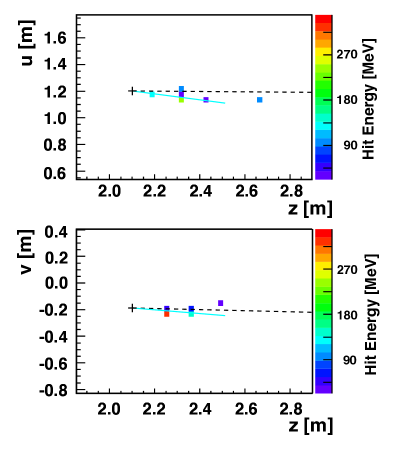
Figure 2: Simulation of coherent $\nu\,+\,\text{Fe}\rightarrow\nu\,+\,\text{Fe}\,+\,\uppi^{0}$ in the Near Detector, showing the locations of hits projected in U-view (upper plot) and V-view (lower plot). The rightmost scale gives the energy deposition in scintillator. Dashed black and solid cyan lines show trajectories of the final state neutrino and $\uppi^{0}$ respectively.

III.2 Data exposure and neutrino flux

The data are obtained from a total exposure of $2.8\times 10^{20}$ POT, from MINOS runs of May 2005 through July 2007. The POT count is accurate to within 1.0% ref:POT_Error . The data set was estimated at the outset to be enough to ensure that the measurement would be limited by systematics rather than statistics. The final results vindicate that estimate; the statistical uncertainties are generally smaller than systematic uncertainties.

A determination of the LE beam $\nu_{\mu}$ flux for the data used in this work was obtained as part of the MINOS measurement of the inclusive CC-$\nu_{\mu}$ cross section ref:CCinclusive . The determination was based upon analysis of a CC subsample characterized by low energy transfer, $\upnu$, to the hadronic system. The data rate in this subsample measures the $\nu_{\mu}$ flux because, in the limit of low-$\upnu$, the differential cross section $d\upsigma^{\nu}/d\upnu$ approaches a constant value independent of $E_{\nu}$ ref:low-nu-method ; ref:D-Bhat_Thesis . Binned values for the $\nu_{\mu}$ flux and uncertainties for $3.0<E_{\nu}<50$ GeV are given in Table II of Ref. ref:CCinclusive .

In a separate determination, the muon fluxes downstream of the beam decay pipe were measured at various target positions and for different horn currents using monitoring chambers deployed in the three rock alcoves. An ab initio simulation of the $\nu_{\mu}$ flux was then adjusted to match the muon flux observations ref:LoiaconoThesis . The two determinations gave similar neutrino fluxes for the the $E_{\nu}$ range above 3.0 GeV where they overlap. For the analysis of this work, the more precise $\nu_{\mu}$ flux determination of Ref. ref:CCinclusive is used for $E_{\nu}>3.0$ GeV, while the $\nu_{\mu}$ flux calculation constrained by measured muon fluxes is used for $E_{\nu}<3.0$ GeV. The neutrino flux integrated from 0.0 to 50 GeV is (2.93$\pm$0.23) $\nu/\text{m}^{2}$/$10^{4}$ POT. The average $E_{\nu}$ is 4.9 GeV and the spectral peak is at 3.0 GeV. The range of neutrino energies about $\langle{E_{\nu}}\rangle$ that contains 68% of the flux is 2.4 $\leq E_{\nu}\leq$ 9.0 GeV. Based upon the measurements reported in Refs. ref:CCinclusive ($E_{\nu}>3.0$ GeV) and ref:LoiaconoThesis ($E_{\nu}<3.0$ GeV), an uncertainty of 7.8$\%$ is assigned to the integrated flux.

IV Coherent NC($\uppi^{0}$) Events

An example simulation of a NC($\uppi^{0}$) coherent interaction in the Near Detector is shown in Fig. 2. A single $\uppi^{0}$ meson of energy 1.31 GeV is produced at a vertex located two scintillator planes upstream of the gamma conversions. The two gamma conversions appear as a single 1.28 GeV electromagnetic shower. In general, electromagnetic showers and hadronic showers of individual events can be distinguished using the reconstructed energy deposition patterns.

Monte Carlo distributions without selections are shown in Figs. 3 and 4 for kinematic variables of Reaction (1). The shaded portions of these distributions denote events that have $E_{vis}$ greater than 1.0 GeV. The remaining events (clear histogram regions) cannot be reliably identified as EM shower events and are excluded from the analysis. The distribution of $\cos\theta_{shw}$ for coherent events (Fig. 3a) is sharply peaked, with 61% of the total sample having $\cos\theta_{shw}>0.97$. The distribution of visible energy, $E_{vis}$, peaks below 1.0 GeV and falls with increasing energy (Fig. 3b). It is predicted that 48% of signal events deposit more than 1.0 GeV, and that 93% have $E_{vis}$ less than 4.0 GeV. The $\cos\theta_{shw}$ and $E_{vis}$ distributions reflect a peaking of signal events at low values of $\eta_{\small{\uppi}}$, as is apparent in Fig. 4, where NC($\uppi^{0}$) coherent events are clustered at $\mbox{$\eta_{\small{\uppi}}$}\leq 0.050$ GeV. Broader $\eta_{\small{\uppi}}$ distributions are predicted for incoherent NC reactions with topologies dominated by EM showers.

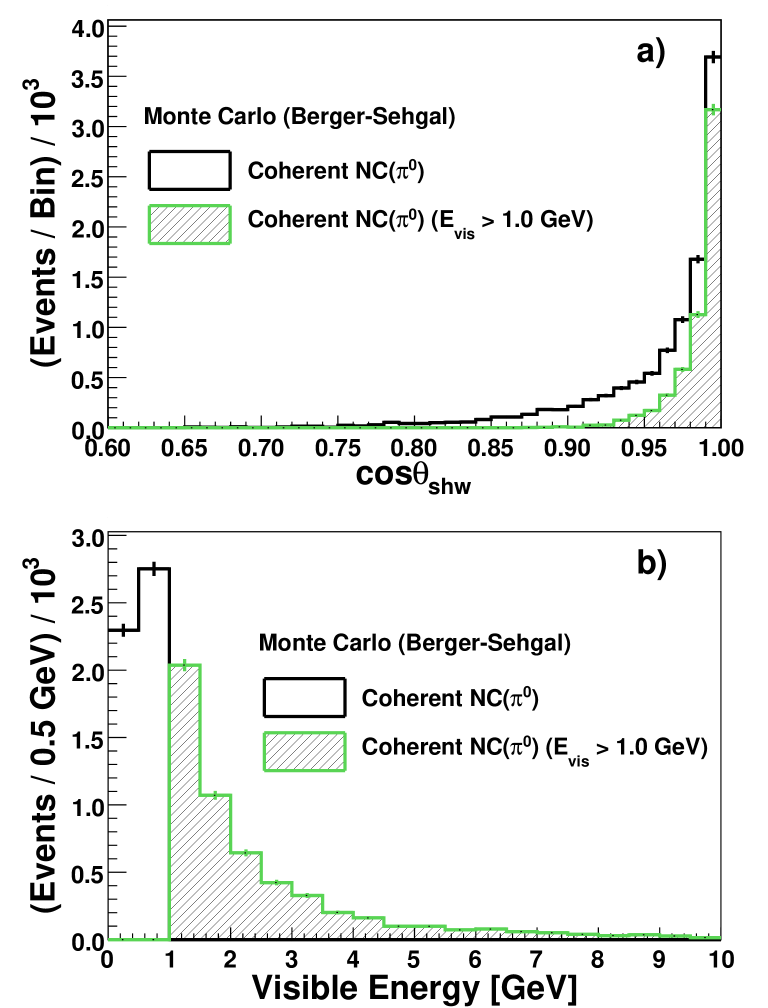
Figure 3: Monte Carlo distributions for NC($\uppi^{0}$) coherent interactions (Berger-Sehgal model) in the Near Detector for the LE beam exposure. (a) Shower-angle cosine of final-state showers with respect to the $\nu$ beam, and (b) Event visible energies. Shaded regions show events with $E_{vis}>1$ GeV.

V Background Reactions

Background interactions originate from one of four neutrino reaction categories, namely NC, CC-$\nu_{\mu}$, CC-$\nu_{e}$, and purely leptonic interactions. It is useful to divide the NC and CC-$\nu_{\mu}$ categories according to the final-state hadronic processes used in MC modeling. The relevant processes are resonance production (RES) and deep inelastic scattering (DIS). Electromagnetic showering particles dominate the reconstructed shower in all of the background categories.

Neutral-current reactions. The dominant background arises from non-coherent NC events with final-state neutral pions that deposit significant shower energy and little additional energy above the MINOS detection thresholds. Their final-state shower angles with respect to the beam, however, are more broadly distributed than those of NC($\uppi^{0}$) coherent scattering.

CC-$\nu_{\mu}$ reactions. There is a subset of CC-$\nu_{\mu}$ events in which the muon track is not identified, and the hadronic shower is dominated by a single $\uppi^{0}$.

CC-$\nu_{e}$ reactions. Beam $\nu_{e}$ ($\bar{\nu}_{e}$) neutrinos can initiate events having single, prompt electrons (positrons) with no evidence of recoil nucleons or other hadronic activity. This CC-$\nu_{e}$ background is mainly composed of quasi-elastic (QE) scattering, however resonance production and DIS processes also contribute. The reconstructed energy distribution peaks at $\sim$2.0 GeV, and extends more broadly to higher energies than the distribution of signal events. Evidence that the MC simulation accurately describes CC-$\nu_{e}$ quasielastic-like events is provided by the differential cross-section measurements of Ref. ref:J-Wolcott-minerva .

Purely leptonic interactions. A small background arises from purely leptonic interactions that initiate energetic single electrons or positrons. It consists of $\nu_{\mu}$-electron scattering, together with much smaller contributions from $\nu_{e}$-electron scattering and from the corresponding antineutrino-electron reactions. These reactions were not included in the NEUGEN3 event generator, and so the neutrino generator GENIE ref:GENIE was used as input to a full simulation. (A check on this GENIE prediction for the NuMI LE beam is provided by a recent MINER$\nu$A measurement ref:J-Park-minerva .) Purely leptonic scattering is estimated to be $1.2\%$ of the selected data sample, and $(9.7\pm 0.8)\%$ of the extracted coherent signal. The background amount, calculated for the data POT exposure, was subtracted from the $\cos\theta_{shw}$-vs-$E_{vis}$ template of the data prior to further analysis steps.

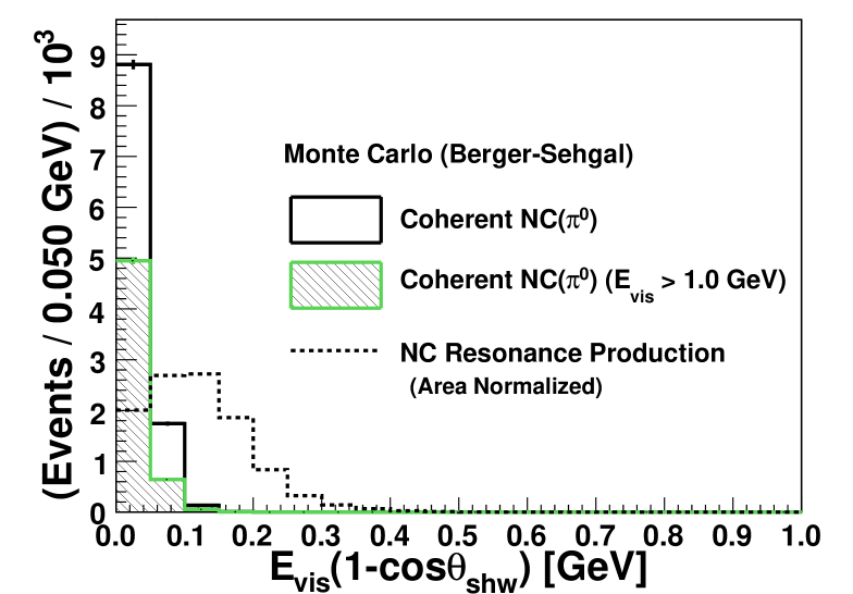
Figure 4: Monte Carlo distribution (solid histogram) of the $\eta_{\small{\uppi}}$ variable for neutrino NC($\uppi^{0}$) coherent interactions from the LE beam exposure. The shaded region shows events with $E_{vis}>1$ GeV. The dashed histogram shows $\eta_{\small{\uppi}}$ for incoherent NC production of resonances that decay into single-$\uppi^{0}$ channels. The latter distribution is shown area-normalized to the signal distribution to elicit differences in shape.

VI Event Selection

A preselection was applied to the data. Events were required to have been recorded when both detector and beamline were fully operational. The shower vertex and cluster of hits were required to be fully contained within the fiducial volume and to have visible energy above 1 GeV. Events with multiple showers, multiple tracks, or single tracks longer than 2 m were rejected. For events that passed the data quality and the fiducial volume containment requirements, the subsequent cut on visible energy removes an estimated 47% of coherent NC($\uppi^{0}$) events. Additional losses of signal are incurred by removal of events having multiple reconstructed showers or having muon-like topologies; the losses are at the sub-percent level for each of the latter cuts. A cutoff was imposed on $E_{vis}$ at 8.0 GeV as few coherent events are predicted to occur above this value. Additionally, $K$-decay rather than muon decay begins to dominate CC-$\nu_{e}$ production above 8.0 GeV. This means that regions above 8.0 GeV are not predictive of background in the signal region and cannot be used as sidebands. This requirement is estimated to remove 2.9% from the total signal (including signal with $E_{vis}<1.0$ GeV).

VI.1 Multivariate algorithm classification

Further isolation of candidate events was achieved using a Support Vector Machine (SVM) classification algorithm. The output of the SVM is a discriminant value assigned to each event, hereafter referred to as the Signal Selection Parameter (SSP). The SVM output for a set of input variables, or “attributes”, was developed from training samples of MC events ref:Cherdack-Thesis . The SVM can accommodate large numbers of input variables whose information content carries various degrees of redundancy; its performance improves in accordance with the total amount of discriminatory information provided. For this analysis, thirty-one different reconstructed quantities were fed to the SVM for each event. The variables represented five categories of information: shower size, shower shape, shower fit, hadronic activity, and track fit. Intentionally omitted were reconstructions of shower direction and shower visible energy. These observables were reserved for use in the fitting of backgrounds to the data.

The SVM algorithm constructs a border surface in the high-dimensional attribute space. The SSP is a measure of “distance” to the border. Signal-like regions and background-like regions receive positive and negative values respectively; locations on the border have a value of zero. Events with energy depositions that have shower-like clusters, are devoid of vertex activity, and have very few remote hits, are to be found in locations having positive and larger SSP values.

Figure 5a compares the SSP distribution of the reference MC sample (histogram) to the unblinded portion of the data (black circles); display of the latter distribution is restricted to SSP $<$ 1.2. The MC signal fraction, or purity, for selected (${\it sel}$) events, $\rho$ = $N^{Coh}_{sel}$/ ($N^{Coh}_{sel}+N^{Bkg}_{sel}$), is displayed as a function of SSP by the dashed line (with scale to the right). Figure 5b shows the SSP region that is enriched with isolated shower events (SSP $>$ 0.9), with the MC simulation broken out into signal and background contributions. For the region in Fig. 5a in the vicinity of SSP = 0 that contains the bulk of the unblinded data, the simulation matches the data to within $5\%$. However Fig. 5b shows that, for the unblinded SSP bins that lie adjacent to the signal-enriched region and contain the black-circle data points, the MC simulation reproduces the slope of the data but predicts a higher event rate. This discrepancy motivates the development of further analysis methods to constrain the background model using data measurements. The data in Fig. 5b displayed with blue-shade circles are shown for completeness; their bins were blinded in the analysis.

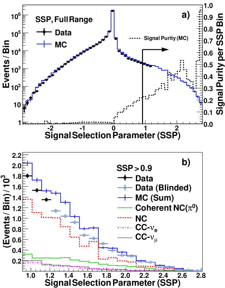
Figure 5: (a) Comparison of SSP distribution (left scale) of the unblinded data (black circles) to the MC prediction (histogram). The unblinded data were restricted to the region with estimated sigal purity $<20\%$; the MC simulation is shown over the full SSP range. The dashed histogram shows the signal fraction per SSP bin (right scale). (b) SSP distributions in an interval of enhanced signal content (denoted by the arrow in (a)). Histograms show the predicted rate broken out into signal and background contributions. In the unblinded portion of the signal-enriched region populated by the black-circle data points, the simulation reproduces the shape but overestimates the rate of the data.

VI.2 Signal-enriched sample and sidebands

The background estimation can be significantly constrained using information available in sideband samples that lie close to the signal phase-space but have low signal content. To this end, selections are used to isolate a signal-enriched sample and to define two separate sideband samples. These selections are made in two stages. In the first stage, a piece-wise linear boundary is defined over the plane of SSP versus $\eta_{\small{\uppi}}$ ref:Cherdack-Thesis . The boundary defines regions in such a way as to isolate samples enriched with certain desired properties. (The specifics of boundary placement are stated below.) Two such regions are defined, one contains the selected sample, and the other contains the near-SSP sample. In the second stage, the events of the two samples are re-binned as a function of $\cos\theta_{shw}$-vs-$E_{vis}$ and are then separated into regions of high purity (the signal region) and of low purity (the sideband). The samples and the selection criteria are elaborated below.

The selected sample: Events are chosen that populate a contiguous region of the SSP-vs-$\eta_{\small{\uppi}}$ plane having highest purity and containing $\geq 10\%$ of estimated coherent signal events. These events (approximately $0.24\%$ of the MC sample shown in Fig. 5a) comprise the selected sample. Specifically, events of the selected sample are required to have SSP $>\,0.5$ for $\mbox{$\eta_{\small{\uppi}}$}\,<0.2$, or else SSP $>\text{max}\{(1.3\,-\,4\times\mbox{$\eta_{\small{\uppi}}$}),\,-\,0.9\}$ for $\mbox{$\eta_{\small{\uppi}}$}>0.2$. (An illustrative plot is available as Fig. 6.2 of Ref. ref:Cherdack-Thesis .)

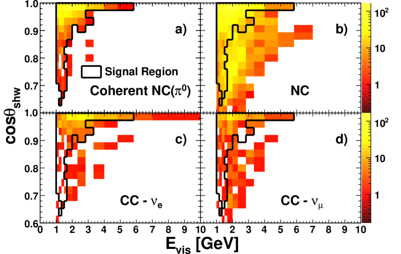
Figure 6: Distributions of the MC selected sample over the $\cos\theta_{shw}$-vs-$E_{vis}$ plane for (a) signal events, (b) the sum of NC resonance plus NC DIS background templates, (c) the CC-$\nu_{e}$ background template, and (d) the sum of CC-$\nu_{\mu}$ resonance and CC-$\nu_{\mu}$ DIS background templates. Bin-by-bin shading (scale on the right) depicts the event populations. The signal region enclosed by the solid-line border shown on all plots is excluded from fitting to the background.

Distributions of the selected MC sample over the $\cos\theta_{shw}$-vs-$E_{vis}$ plane, shown separately for signal and backgrounds, are plotted in Fig. 6. The black-line border separates the bins into two regions according to their signal purity as described below. A large fraction of the sample consists of background events; the relatively large contribution from NC background can be seen in Fig. 6b.

• Selected sample, signal region: The region of the $\cos\theta_{shw}$-vs-$E_{vis}$ plane with bins predicted to have $\rho>5\%$, comprises the signal region of the analysis. Its outer boundary is shown by the black-line border superposed on the $\cos\theta_{shw}$-vs-$E_{vis}$ distributions of Fig. 6.

• Selected sample, sideband: The selected-sample population lying outside of the signal region on the $\cos\theta_{shw}$-vs-$E_{vis}$ plane is predicted to have bins with $\rho<5\%$. These events provide information concerning signal-like backgrounds; they comprise the sideband portion of the selected sample.

The near-SSP sample: A second sample, designated the near-SSP sample, populates regions adjacent to, but on the opposite side of, the border previously specified that encloses the selected sample on the SSP-vs-$\eta_{\small{\uppi}}$ plane. Like the selected sample sideband, the near-SSP also contains signal-like background events. Its inclusion provides additional statistical power to the background fits.

• Near-SSP, sideband: There is a region of the near-SSP $\cos\theta_{shw}$-vs-$E_{vis}$ plane where the binned event populations have $\rho<5\%$ in each bin. The events that are contained in this region comprise the near-SSP sideband sample.

• Near-SSP, excluded region: The remainder of the near-SSP has purity above 5% and is excluded from the near-SSP sideband. The purity in this region is too low for use as a signal region, as uncertainties on the subtracted backgrounds overwhelm the modest gains from statistics. Consequently this subsample is excluded from the analysis altogether.

As part of the blinding protocol, data in the two sideband samples were not investigated until the sideband fitting procedure was fully developed based on mock data studies. Similarly, the data in the signal region were not evaluated until the fit to the sideband samples was complete, and the background rates in the signal region and their associated uncertainties were fully determined.

As elaborated in Sec. VII, the templates comprising the background model are tuned via fitting to match the data of the sideband samples. The background estimate to be subtracted from the data is thereby anchored in the sidebands but it also encompasses the signal region. The number of data events in the signal region that exceed the estimated background population, represents the coherent scattering signal.

Figure 7 shows the distributions of $\cos\theta_{shw}$ and $E_{vis}$ for the MC selected sample, normalized to the data exposure. These depict projections of the distributions shown in Fig. 6. The sample contains 935 coherent NC($\uppi^{0}$) events (19.1% of the sample), together with 3,960 background events. The composition of the background is 81.8% NC, 9.3% CC-$\nu_{\mu}$, and 8.9% CC-$\nu_{e}$.

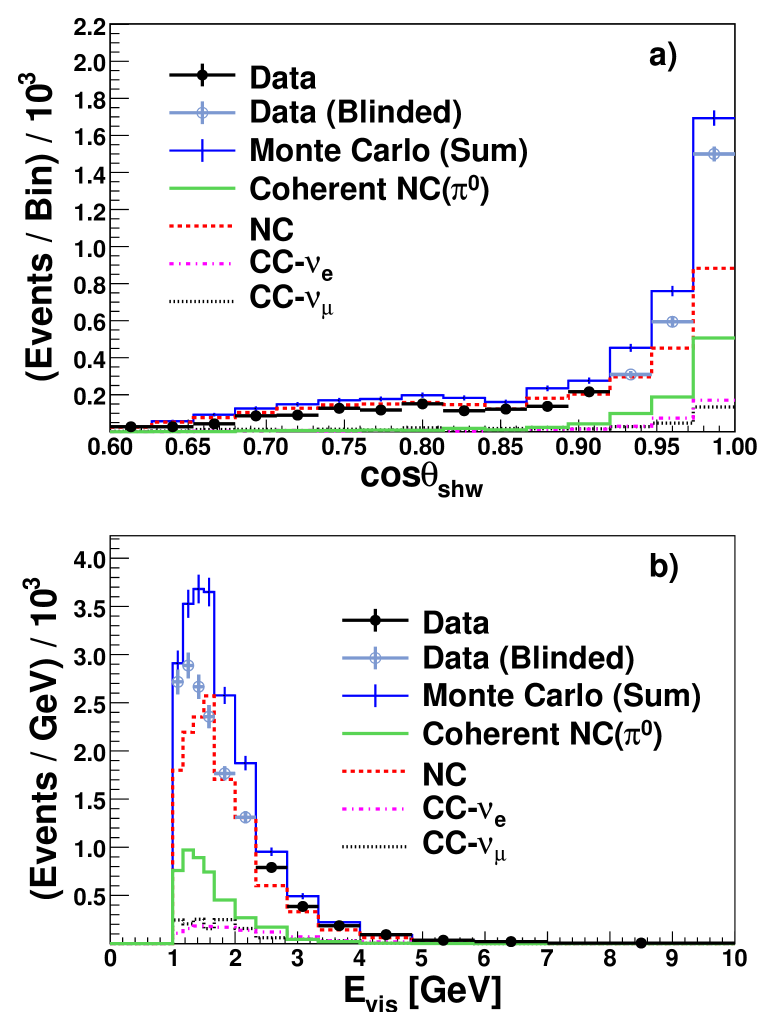
Figure 7: Distributions of reconstructed (a) $\cos\theta_{shw}$ and (b) $E_{vis}$ for the data (circles, statistical errors) and MC (histograms) of the selected sample. Data shown as black circles are in the unblinded regions $(\rho<20\%)$. The reference MC matches the shape but exceeds the rate of the unblinded data.

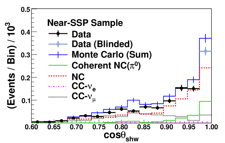
Figure 8: Distribution of reconstructed $\cos\theta_{shw}$ for data (circles) and the reference MC (histograms) of the near-SSP sample. In the background dominated regions at larger angles, the MC predicts the shape but overestimates the rate of the data.

Figure 8 shows the $\cos\theta_{shw}$ distribution of the near-SSP sample including the sideband and the excluded region. Compared to the selected-sample sideband, the near-SSP sideband has lower event statistics, however its lower purity allows a larger number of $\cos\theta_{shw}$-vs-$E_{vis}$ bins to be included. Roughly speaking, the near-SSP sideband includes bins with $\eta_{\pi}\geq 0.1$ while the selected-sample sideband restricts to bins that satisfy $\eta_{\pi}\geq 0.2$. In both Fig. 7 and Fig. 8, the data shown by the solid circles are in the unblinded regions, while the data displayed as blue-shade circles were blinded. For the unblinded data, the MC simulation is seen to overestimate the rate of selected data events by $\sim 35\%$. It will be shown that this discrepancy is removed by adjusting the background models, within uncertainties, to match data rates observed in the sideband samples.

VII Background Estimation by Fitting to Data

Central to the analysis is its background fitting procedure which delivers an effective accounting of most of the systematic uncertainties of the measurement using relatively few parameters. Sections VII through X describe its design and performance.

VII.1 Fit normalization parameters

For each background category, two separate MC templates containing either selected or near-SSP events are constructed as two-dimensional $\cos\theta_{shw}$-vs-$E_{vis}$ histograms. The bin sizes are set according to experimental resolutions. Bins of $E_{vis}$ are proportional to its residual, $|\,E_{vis}-E_{true}|$, and enlarge with energy to match the resolution dependence (residual/$E_{true}\sim$20%). For $\cos\theta_{shw}$, its residual over the sample is nearly constant and so a constant bin-width of 0.04 is used. The MC templates, together with similar histograms of the data, are the principal inputs to the fit.

Figure 6 shows the MC $\cos\theta_{shw}$-vs-$E_{vis}$ distributions of selected-sample events for the signal (Fig. 6a) and for the background reaction categories: NC (Fig. 6b), CC-$\nu_{e}$ (Fig. 6c), and CC-$\nu_{\mu}$ (Fig. 6d). Events enclosed by the solid-line border lie in the signal region while events lying outside belong to the sideband. As previously noted, the NC and CC-$\nu_{\mu}$ categories are further divided by the analysis into sub-categories that distinguish baryon resonance production and DIS interactions.

Associated with each background reaction category there is a normalization parameter; it serves to scale the total number of events assigned to the template distribution of the background. Studies of fitting using simulated data experiments showed the normalization parameters for the templates of CC-$\nu_{\mu}$ resonance production and NC resonance production to be highly correlated. Strong correlations were also observed for the CC-$\nu_{\mu}$ DIS and NC DIS templates. Thus it was decided to combine each of these pairs of background categories, allowing for each pair a single template scaled by a normalization parameter. Three templates with independent normalizations then suffice to describe the backgrounds: i) NC and CC-$\nu_{\mu}$ resonance production events; ii) NC and CC-$\nu_{\mu}$ DIS events; and iii) CC-$\nu_{e}$ events. Hereafter, the corresponding normalization parameters are designated using $n_{res}$, $n_{dis}$, and $n_{\mbox{$\nu_{e}$}}$.

If a systematic error causes the template normalizations to change, but not the shapes of the $\cos\theta_{shw}$-vs-$E_{vis}$ distributions, then that error can be absorbed into the normalization parameters. It was demonstrated using simulated experiments (see Sec. IX.4) that most sources of systematic uncertainty can be accounted for in this way. This approach simplifies the treatment and promotes the identification of a minimal set of effective systematics parameters.

There are two systematic uncertainty sources that can significantly alter the shapes of the template distributions, namely the energy scale for EM showers and the assignment of the Feynman scaling variable ($x_{F}$) to final-state nucleons. These sources must be fit for independently, and each requires a systematic parameter (Sec. IX.4).

VII.2 Limiting the signal content of sidebands

It is observed with simulated experiments that signal events in sideband samples bias the determination of the number of coherent NC($\uppi^{0}$) events toward the MC prediction. It is important to minimize this influence by defining the sidebands such that only bins with low signal purity are included. On the other hand, limiting the number of bins in the sidebands reduces the amount of information available to the fit. As a compromise, the estimated signal purity of bins in the sidebands was required to be less than 5%. With the latter requirement, this bias, inherent to the analysis fitting procedure, is a small effect of 5.8%. Its contribution to the signal rate is corrected for, and the uncertainty arising from the correction is propagated to the error budget.

VII.3 The $\chi^{2}$ fit to the background

Best-fit values for the background normalization parameters $n_{res}$, $n_{dis}$, and $n_{\mbox{$\nu_{e}$}}$ plus two systematic parameters (Sec. IX.4) that allow for shape distortions of the background templates, are determined by minimization of the $\chi^{2}$:

$$\begin{split}\chi^{2}=2\displaystyle\sum_{i}\left[\left(\ln\displaystyle\frac{N^{Data}_{i}}{N^{MC}_{i}}-1\right)N^{Data}_{i}+N^{MC}_{i}\right.\hskip 36.135pt\\ +\left.\left(\ln\displaystyle\frac{N^{MC}_{i}}{N^{adj}_{i}}-1\right)N^{MC}_{i}+N^{adj}_{i}\right]+~{}\text{penalty}~{}\bf{.}\end{split}$$ (5)

The $\chi^{2}$ summation is taken over the bins, $i$, of the selected and near-SSP sideband regions of the $\cos\theta_{shw}$-vs-$E_{vis}$ plane. The first two terms within the brackets of Eq. (5) represent the likelihood that, according to Poisson statistics, the number of data events of bin $i$ agrees with the number of events predicted by the MC simulation. Here, $N^{Data}_{i}$ is the number of data events observed in bin $i$, and $N^{MC}_{i}$ is the number of events expected in the same bin for a given set of values for the five parameters of the fit.

Due to the relatively low rate of coherent NC($\uppi^{0}$) interactions and their associated backgrounds, the selected sample – although extracted from very large MC samples – has limited statistics. This problem is addressed by introducing the third and fourth terms constructed according to the method of Beeston and Barlow ref:limitMCstats . In brief, the MC content of each bin arising from all the MC samples is fitted to the corresponding data so that the sum of terms three and four in (5) is minimized for each bin. The logarithmic term imposes a cost for the adjustment of the MC simulation from $N^{MC}_{i}$ to its corresponding fitted value, $N^{adj}_{i}$. The inclusion of the latter terms effectively replaces $N^{MC}_{i}$ with $N^{adj}_{i}$ plus the penalty.

An additional penalty term in the $\chi^{2}$ constrains the values of the fit parameters; the constraints are based upon the studies of systematic uncertainties discussed in Sec. IX.4. The penalty term is constructed using a covariance matrix which encodes the variations allowed to the vector of fit parameters, $\hat{\delta}$, as related in Sec. IX.5:

$${\mathrm{penalty}}=\vec{\delta}\cdot(V)^{-1}\cdot(\vec{\delta})^{T}\bf{.}$$ (6)

Multiple covariance matrices were formulated to allow for asymmetries in the parameter errors. The appropriate matrix is chosen based on the sign of the normalization parameter deviations.

VIII Extraction of the Signal Rate

Minimization of the $\chi^{2}$ yields the best-fit values for the fit parameters, and these are used to estimate the rate for each category of background events across the entire selected sample.

VIII.1 Raw signal event rate

The number of selected events (in bin $i$) contributed by background template $b$ is $N_{ib}^{MC}$. Each $N_{ib}^{MC}$ is scaled by a background normalization parameter, $f_{b}$ = $n_{res}$, $n_{dis}$, or $n_{\mbox{$\nu_{e}$}}$, and the systematic scale factor, $s_{ib}$. The value of $s_{ib}$ is the sum of fractional changes (bin-by-bin) induced by changes in value for systematic parameters associated with uncertainties of EM energy scale and of $x_{F}$ assignment to final-state nucleons (see Sec. IX.4). The predicted number of background events in each bin $N^{Bkg}_{i}$, is the sum of the scaled values of $N_{ib}^{MC}$ over the three background templates:

$$N^{Bkg}_{i}=\displaystyle\sum_{b}f_{b}\,s_{ib}\,N_{ib}^{MC}\bf{.}$$ (7)

The measured signal in each bin, $N^{Coh}_{i}$, is the difference between the number of data events and the number of neutrino background events as estimated using Eq. (7):

$$N^{Coh}_{i}=N^{Data}_{i}-N^{Bkg}_{i}\bf{.}$$ (8)

The background subtraction yields a count of measured signal events in each bin of the selected sample.

VIII.2 Acceptance corrections

The acceptance correction is applied via an efficiency function,

$$\epsilon_{i}=\frac{N^{MCs}_{i}}{N^{MCt}_{i}}\textbf{ ,}$$ (9)

where $N^{MCs}_{i}$ is the number of coherent NC($\uppi^{0}$) MC events in bin $i$ in the selected sample and $N^{MCt}_{i}$ is the total number of coherent NC($\uppi^{0}$) events in bin $i$ predicted by the reference MC.

There are a small number of bins for which very few signal events are estimated and the efficiency approaches zero. These bins are omitted from the sum-over-$i$ and their correction is applied via an overall factor $\epsilon_{0}^{-1}$, calculated as the ratio of the (predicted) total signal rate divided by the selected signal rate for all bins with non-zero efficiency. The choice of an acceptance correction for each bin, either bin-by-bin ($\epsilon_{i}$) or overall ($\epsilon_{0}$), was determined by minimizing the uncertainty propagated to the measured signal. Also included in $\epsilon_{0}$ is the correction for signal loss incurred by the $E_{vis}<8.0$ GeV cutoff, and a small correction for interactions that were not properly reconstructed.

There are coherent NC($\uppi^{0}$) MC events with true visible energy below 1.0 GeV that reconstruct with $E_{vis}>1.0$ GeV, and vice versa. An additional correction is applied as a weight factor, $\xi$, to account for the net event migration across the cut boundary at $E_{vis}=1.0$ GeV. The acceptance-corrected coherent event rate is then

$$N^{Coh}=\frac{\xi}{\epsilon_{0}}\displaystyle\sum_{i}^{\epsilon_{i}>0}\frac{1}{\epsilon_{i}}\Bigg{(}N^{Data}_{i}\,-\left.\displaystyle\sum_{b}f_{b}\,s_{ib}\,N_{ib}^{MC}\right)\,\bf{.}$$ (10)

The integrated effect of the bin-by-bin acceptance corrections $\epsilon_{i}^{-1}$ in the summation of Eq. (10) is equivalent to to an overall correction of about 8.2. The factors $\epsilon_{0}^{-1}$ and $\xi$ in Eq. (10) introduce corrections of 1.42 and 0.90 respectively; their net effect is to shift the calculated signal rate upward by $28.1\%$.

IX Systematic Uncertainties

Sources of systematic uncertainties are described below. The effects of individual sources are summarized in Sec. IX.4. Many of the sources were studied in previous MINOS analyses ref:MINOS_nue ; ref:POT_Error .

IX.1 Uncertainties in neutrino-interaction modeling

Modeling of $\nu$N cross sections: The dominant uncertainties in the cross section model are associated with $i$) the axial mass $M^{QE}_{A}$ used in quasielastic cross sections, $ii$) the axial mass $M^{Res}_{A}$ used in resonance production cross sections, and $iii$) the treatment of the transition region between resonance production and DIS ref:neugen3 ; ref:D-Bhat_Thesis . The values and $\pm 1\upsigma$ uncertainties of the model parameters were taken from previous MINOS investigations ref:POT_Error ; ref:CCinclusive . The axial masses $M^{QE}_{A}$ and $M^{Res}_{A}$ used with dipole form factors are effective parameters whose assigned fractional errors makes allowance for uncertainties arising from nuclear medium effects neglected by the MC such as 2-particle 2-hole excitations and long-range correlations martini-2p2h ; valencia-2p2h .

Modeling of hadronization: Uncertainties in the NEUGEN3 hadronization model reflect a lack of data on the DIS channels selected by the analysis. Six model parameters were identified as having uncertainties that influence the predicted event samples and their effects were individually investigated: i) The assignment of Feynman-$\mathit{x}$ to the final-state baryon, $\mathit{x_{F}}$; ii) the probability for $\uppi^{0}$ production, $\mathit{P(\mbox{$\uppi^{0}$})}$; iii) the correlation between produced neutral-particle multiplicity and charged-particle multiplicity, $\mathit{n_{0}}$ and $\mathit{n_{\pm}}$, respectively; iv) differences between generator simulations of hadronic systems, gen-diff, (GENIE ref:GENIE vs NEUGEN3 ref:neugen3 ); v) damping algorithm for transverse momenta, $\mathit{p_{\small{T}}~{}damping}$; and vi) neglect of correlations which may arise with two-body decays, $\mathit{decay~{}param}$.

Intranuclear rescattering:

Neutrino-induced pions and nucleons can undergo final-state interactions (FSI) prior to emerging from the parent nucleus. The analysis accounts for FSI processes in all incoherent neutrino scattering interactions using a cascade model to simulate the propagation of produced hadrons within the target nuclei ref:Intranuke-Model . For coherent signal reaction (1) however, the rate and final-state momenta of produced $\uppi^{0}$s in simulation are taken directly from the Berger-Sehgal model. The model accommodates the attentuation of coherently produced $\uppi^{0}$s by the parent nucleus by using pion-nucleus elastic-scattering cross sections as input ref:BS .

The performance of the FSI cascade model is governed by two types of adjustable parameters. The first type establishes relative rates for the possible intranuclear processes with $\pm 1\upsigma$ as evaluated for the MINOS analysis of $\nu_{\mu}$ disappearance ref:POT_Error . The seven parameters of the first type are i) pion charge exchange, ii) pion elastic scattering, iii) pion inelastic scattering, iv) pion absorption, v) $\uppi$-nucleon scattering yielding two pions, vi) nucleon knockout from the target nucleus, and vii) nucleon-nucleon scattering with pion production. Parameters of the second type govern the overall rate of intranuclear rescattering, e.g. the pion-nucleon cross section and the formation time, $\mathit{T_{formation}}$, for directly produced hadrons.

IX.2 Implications for background reactions

NC reactions: Generation of NC events is affected by all of the above-listed modeling uncertainties  ref:CalDet-2006 ; ref:T-Yang_Thesis ; ref:Boehm_Thesis .

CC-$\nu_{\mu}$ reactions: The cross sections for CC-$\nu_{\mu}$ reactions are better-known and hence better-constrained than for NC channels. Moreover the selected CC-$\nu_{\mu}$ rate is only 10% of the selected NC event rate. Consequently the effects of uncertainties with modeling of CC-$\nu_{\mu}$ interactions are sufficiently weak to be subsumed by the error range assigned by the fit to the $n_{res}$ and $n_{dis}$ normalization parameters (see Sec. IX.4).

CC-$\nu_{e}$ reactions: The electron-induced showers of selected CC-$\nu_{e}$ events have no visible hadronic activity, and so uncertainties arising from hadronization and intranuclear rescattering are negligible. The dominant uncertainty in the CC-$\nu_{e}$ event rate arises from limited knowledge of the ($\nu_{e}+\bar{\nu}_{e}$) flux in the NuMI LE beam ref:MINOS_nue ; ref:Ochoa_Thesis . The additional 20% flux uncertainty is propagated to the uncertainty assigned to the $\nu_{e}$ normalization parameter.

IX.3 Uncertainties of energy scale and signal model

Uncertainties in the electromagnetic energy scale, $\mathit{E_{scale}^{EM}}$, and detector calibration contribute significantly to the error budget. An overall uncertainty of $\pm$5.6% is assigned to the EM energy scale, reflecting uncertainty with hadronic contributions to MINOS shower topologies ($\pm 5.1\%$), together with uncertainties in the detector response to EM showers ($\pm$2.0%). The latter response was evaluated using measurements obtained with the MINOS Calibration Detector ref:Boehm_Thesis .

Inaccuracies in modeling the coherent-scattering signal can influence the signal amounts inferred from the background levels established by fitting. Signal model inaccuracies also enter into the acceptance corrections. The effect was evaluated using simulated experiments employing alternate models of the coherent interaction cross section ref:Cherdack-Thesis . The definitions of the signal region and sidebands, by design, minimize the influence of the signal model. The net effect to the signal rate is accounted for by the uncertainty on the $5.8\%$ sideband biasing correction of Sec. VII.2 plus the $\pm$3.2% uncertainty attributed to the acceptance corrections of Sec. VIII.2.

IX.4 Evaluation of sources

The effect of each source of systematic uncertainty was evaluated individually. Monte Carlo samples were created in which a single input parameter, corresponding to one of the sources (Sec. IX A,C), was changed by its $\pm$1$\upsigma$ uncertainty. The $\cos\theta_{shw}$-vs-$E_{vis}$ distribution of each altered sample was then compared to the background model. Fitting the sidebands of the background templates to the sidebands of the altered MC sample yields a re-expression of the $\pm 1\upsigma$ uncertainties on the underlying model parameters as uncertainties on template normalizations. However, for systematic uncertainties that induce changes in the background templates that cannot be adequately described by normalization changes, use of their underlying model parameters is retained and their effects on the normalization parameter uncertainties are not included.

For each of the above-described exercises the altered MC distribution was treated like “data”, thus the altered MC samples are referred to as Single-Systematic Mock Data (SSMD). The overall campaign was to generate SSMD samples for each systematic, subject each sample to the template fit procedure that constrains the background model in the sidebands, and evaluate the outcomes. Evaluations external to the fitting are used for systematic uncertainties associated with calibration (see Sec. XI).

More specifically, the steps were as follows: i) For each source of uncertainty, fluctuations of $\pm 1\upsigma$ in the corresponding parameter induce changes to the SSMD event distribution in $\cos\theta_{shw}$-vs-$E_{vis}$; ii) the changes in the event distribution are evaluated by fitting the background model to the fluctuated distribution, allowing the three background normalization parameters $n_{res}$, $n_{dis}$, and $n_{\mbox{$\nu_{e}$}}$, to float without restriction; iii) the SSMD fit result is used to identify whether or not a source introduces a shape change into the $\cos\theta_{shw}$-vs-$E_{vis}$ spectrum. iv) In the cases where the systematic uncertainty does not induce a significant shape change (most do not), the best-fit values of the SSMD fit are used to calculate the allowed variances on (and covariance between) the normalization parameters in the final analysis fit to sideband data.

For each source of systematic uncertainty, the shifts $-1\upsigma$, $+1\upsigma$ were considered separately. The fitting to SSMD samples provided the $\chi^{2}/ndf$ for the best fit, the fit values for the normalization parameters, and the extracted signal, which was compared to the value for the reference MC. Since each SSMD sample is created by inducing a $1\upsigma$ change in a single systematic parameter, and does not include any statistical fluctuations, the $\chi^{2}/ndf$ is rated against 0.0 rather than the usual 1.0.

For fifteen of the twenty-two systematic error sources, the SSMD trials yielded $\chi^{2}/ndf<0.05$, well-understood deviations of background normalizations from their nominal values, and extracted signal event counts which were within $\pm 19\%$ of the simulation “truth” values. Thus, in fitting the background model to data, shifts of these fifteen sources can be absorbed by the normalization parameters. Typical of these fifteen “well-behaved” sources is the axial-vector mass, $\mathit{M_{A}^{Res}}$, which is here singled out as an example. The results from an SSMD trial wherein $\mathit{M_{A}^{Res}}$ was subjected to a +1 $\sigma$ shift are summarized in the bottom row of Table 2.

Systematic	Shift	Best-Fit Norm.			Fit Outcome
		NC+CC$\nu_{\mu}$		CC$\nu_{e}$	$\bf{\chi^{2}}/ndf$	Signal
Source		$n_{res}$	$n_{dis}$	$n_{\mbox{$\nu_{e}$}}$		Ratio
$\mathit{E_{scale}^{EM}}$	-5.6%	1.13	0.75	0.85	1.32	1.45
$\mathit{E_{scale}^{EM}}$	+5.6%	1.00	1.20	1.33	0.79	0.91
$\mathit{x_{F}}$	+1 $\upsigma$	1.45	0.83	0.97	0.78	0.30
$\mathit{n_{0}(n_{\pm})}$	$\pm$1 $\upsigma$	1.15	0.83	0.78	0.18	0.92
$\mathit{decay~{}param.}$	+1 $\upsigma$	1.15	0.85	0.90	0.15	0.78
$\mathit{gen-diff}$	$\pm$1 $\upsigma$	1.03	0.95	0.80	0.13	0.87
$\mathit{p_{\small{T}}~{}damping}$	$\pm$1 $\upsigma$	1.00	0.98	0.78	0.12	0.88
$\mathit{T_{formation}}$	-50%	1.00	0.88	0.85	0.10	0.94
$\mathit{T_{formation}}$	+50%	1.08	1.05	1.10	0.07	1.32
$\mathit{M_{A}^{Res}}$	+15%	1.83	1.00	1.10	0.02	1.01

Table 2: Summary of SSMD studies of uncertainty sources having potential to alter the shape of $\cos\theta_{shw}$-vs-$E_{vis}$ distributions. Shown are the effects of -1$\upsigma$ and +1$\upsigma$ changes in the sources on the three normalization parameters, together with the $\chi^{2}$ and the ratio of the extracted signal to the true signal. Deviations of the fit parameters and signal ratio are relative to the nominal value of 1.0 for the reference MC. The EM energy scale and $x_{F}$ of the hadronization model exhibit the most significant effect on the expected number of events as a function of $\cos\theta_{shw}$-vs-$E_{vis}$.

IX.5 Systematic parameters; fit penalty term

For the remaining systematic sources shown in Table 2, somewhat larger $\chi^{2}/ndf$ or excursions of the measured event rates from the reference MC values were observed. Table 2 lists the SSMD fit results for each of the latter sources of uncertainty; the sources are ranked according to the reduced $\chi^{2}$. In particular, three of 1$\upsigma$ shifts in two sources have $\chi^{2}/ndf$ which are distinctly worse than the rest. The sources are the EM energy scale (large $\chi^{2}/ndf$ for both -1$\upsigma$ and +1$\upsigma$ shifts), and the parameter associated with assignment of $x_{F}$ to nucleons of final-state hadronic systems (large $\chi^{2}/ndf$ for +1$\upsigma$ shift). Their SSMD fit results are displayed in the first three rows of Table 2.

The $\chi^{2}/ndf$ values of Table 2 provide guidelines for the introduction of additional systematic parameters that may entail distortions to template shapes. Studies utilizing ensembles of “realistic” mock data experiments (see the Appendix) examined the performance of fit-parameter configurations wherein various combinations of parameters listed in Table 2 were introduced. The width of the ($N_{fit}-N_{input}$) spectrum obtained from each mock data ensemble was used as the figure-of-merit for distinguishing among parameter sets. It was observed that the width was reduced with addition of a systematic parameter to account for variation in the EM energy scale, and was further reduced when a systematic parameter to account for variation in the assignment of $\mathit{x_{F}}$ to final-state nucleons was included. Neither the addition of more parameters nor the utilization of other shape parameter combinations yielded a further decrease in the spectral width.

The aggregate of $\pm 1\upsigma$ uncertainty from the ensemble of sources of systematic uncertainty evaluated by the SSMD trials determines the correlated ranges of variation to be allowed to the background normalization parameters. This greatly reduces the number of systematic parameters that, if otherwise included, would exert degenerate effects on the predicted background $\cos\theta_{shw}$-vs-$E_{vis}$ distributions. The resulting fit to data sidebands is less susceptible to multiple minima and less dependent on the details of the background cross section models. The above-mentioned ranges are enforced in the fit $\chi^{2}$ of Eq. (5) by the penalty term of Eq. (6).

X Fitting to Data Sidebands

A simultaneous fit over the data of the selected-sample and near-SSP sidebands is now carried out via minimization of the $\chi^{2}$ function of Eq. (5). The $\chi^{2}$ uses the three background normalization parameters and the two systematic parameters in conjunction with the fit penalty term as described in Sec. VII. The fit result establishes the background prediction in the signal region of the selected sample. The outcome of the fit is illustrated in Fig. 9. Here, data of the selected sample is compared to the neutrino background model for the $\cos\theta_{shw}$ projection of the sideband region of the $\cos\theta_{shw}$-vs-$E_{vis}$ plane. The shapes of the distributions in Fig. 9 reflect the irregular contour of the sideband region (as indicated by Fig. 6). Figure 9a shows the $\cos\theta_{shw}$ projection prior to fitting. The neutrino NC category is the dominant background; its distribution (dashed line) approximates the shape of the sideband data (solid circles), however its normalization is too high by $\sim 35\%$ as noted in Sec. VI.

Figure 9b shows the best fit (solid line histogram) together with the background composition. The fit reduced the normalizations $n_{res}$ and $n_{dis}$ by -1.04 $\upsigma$ and -1.08 $\upsigma$ respectively (corresponding to 35% and 25% reductions), while increasing $n_{\mbox{$\nu_{e}$}}$ by +0.40 $\upsigma$ (a 17.5$\%$ increase). Additionally the EM energy scale is shifted upwards by +0.15 $\upsigma$, corresponding to a 0.84% increase in the conversion from energy deposition in the detector to the measured energy in GeV. The best-fit value for baryonic $x_{F}$ corresponds to a +0.35$\upsigma$ shift from nominal. This change increases the probability that the final-state nucleon will emerge in the forward hemisphere of the target rest frame.

The fit to the data gives a reduced $\chi^{2}$ lower than the values obtained in 52.7% of the realistic mock data experiments described in the Appendix, indicating that the MC simulation is representative of the data to within the MC uncertainties. Comparisons of the best-fit background to the $E_{vis}$ projection of the selected data in the sideband, and to the $\cos\theta_{shw}$ and $E_{vis}$ projections of the near-SSP data sample, also show a satisfactory description of the data ref:Cherdack-Thesis ; ref:Cherdack-NuInt11 .

Figure 9: Distribution in $\cos\theta_{shw}$ for selected data (solid circles) in the sideband region of the $\cos\theta_{shw}$-vs-$E_{vis}$ plane. (a) Data versus MC background templates prior to fitting. (b) Data compared to background of the best-fit MC. The fit adjustment reduced the NC background (dashed) and increased the $\nu_{e}$ background (dot-dashed) to achieve a good description (thick-line histogram).

XI Signal Rate and Uncertainty Range

With the best fit over the data sidebands in hand, the background is set for the entire $\cos\theta_{shw}$-vs-$E_{vis}$ plane. At this point the background prediction is fully determined and the data of the signal region is unblinded.

Figure 10 shows the distributions in $\cos\theta_{shw}$ (Fig. 10a) and in $\eta_{\small{\uppi}}$ (Fig. 10b) for all selected data. The predicted background (clear histogram) shows good agreement with the data points (solid circles) over the lower range ($<\,0.9$) of $\cos\theta_{shw}$ and over the upper range ($>0.25$) of $\eta_{\small{\uppi}}$. The signal for Reaction (1) emerges with either variable as the incident neutrino direction is approached, appearing as a data-minus-background excess (shaded histograms). The errors on the extracted signal are the quadrature sum of errors from the background fit plus statistical uncertainties of the data and MC.

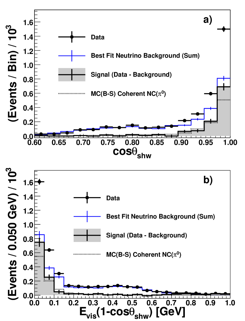
Figure 10: Distributions of candidate NC($\uppi^{0}$) coherent scattering events (solid circles, statistical error bars) in $\cos\theta_{shw}$ (a) and $\eta_{\small{\uppi}}$ (b). The data are compared to the estimate for the neutrino backgrounds (thin blue-line histograms). The coherent scattering signal (data minus background) is shown by the shaded histogram, together with the signal rate inferred using the Berger-Sehgal model (dotted histogram).

Signal events are accepted into the selected sample with an efficiency of $10.7\%$. (The total acceptance, accounting for loss due to the $E_{vis}<1.0$ GeV threshold cut, is estimated to be $4.6\%$). The correction to the measured event rate is implemented as prescribed by Eq. (10). Figure 11 shows the acceptance-corrected signal as a function of $\eta_{\small{\uppi}}$ (shaded histogram) for all events having $E_{vis}>1.0$ GeV. Error bars on the binned signal are the quadrature sum of background uncertainties, statistical errors, and uncertainty with acceptance correction factors. In Fig. 11 the coherent-scattering signal is almost entirely confined to the range $0.0<\mbox{$\eta_{\small{\uppi}}$}<0.2$ in agreement with the general trend predicted by the Berger-Sehgal model (dotted-line histogram). However the data exceed the model’s prediction by nearly 2 $\sigma$ for $0.0<\mbox{$\eta_{\small{\uppi}}$}<0.1$, while falling below the prediction for $0.1<\mbox{$\eta_{\small{\uppi}}$}<0.2$. These features suggest that the coherent interaction may be more sharply peaked towards $\mbox{$\eta_{\small{\uppi}}$}=0$ than is predicted by Berger-Sehgal.

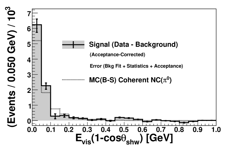
Figure 11: Distribution in $\eta_{\small{\uppi}}$ for the acceptance-corrected data excess above the total neutrino background rate, for events having $E_{vis}>1.0$ GeV (shaded histogram). The dotted-line histogram shows the Berger-Sehgal prediction.

The largest uncertainty of $N^{Coh}$ arises from the estimation and subtraction of background events. The constraints on the normalization and systematic parameters obtained from the fit to the sidebands are the 1$\upsigma$ confidence intervals extracted from the profiled 1-D $\Delta\chi^{2}$ distributions. The uncertainty due to the background subtraction is calculated from the minimum and maximum background rates allowed by the fit-parameter ranges. Propagation of the 1$\upsigma$ CL interval limits on the background to the final measurement results in an error band of (+11.6%, -14.4%).

The signal model enters into the calculation of $N^{Coh}$ in the acceptance corrections, and in the calculation of the signal in the sidebands. The bin-by-bin acceptance correction factors for events with $E_{vis}>1.0$ GeV incur statistical uncertainties from the reference signal MC and shape uncertainties due to finite bin widths. This contributes an additional $\pm$3.2% uncertainty and increases the total error band to (+12.0%, -14.8%). A larger signal-model dependence enters via the correction factor used to estimate the number of events having $E_{vis}<1.0$ GeV. An uncertainty estimate is presented in Sec. XII.

Biasing of the extracted signal towards the signal-model prediction (5.8%) is corrected by scaling the measured signal amount away from the MC prediction by 5.8%. The uncertainty introduced by this correction is listed in the second row of Table 3. Then the total extracted signal is $N^{Coh}$ = 9,550 events. The percentage error range calculated for $N^{Coh}$ at this stage is (+12.6%/-15.5%), in good agreement with an estimate based upon mock data experiments of $\pm 15.8\%$ (see Appendix). The coherent NC($\uppi^{0}$) signal is 12.8% higher than, but within 1$\upsigma$ of, the Berger-Sehgal prediction.

There is uncertainty in the subtraction of the estimated background from purely-leptonic neutrino-electron scattering ($\pm 0.8\%$). Additionally the signal sample may incur a small contribution from diffractive scattering of neutrinos on hydrogen ref:diffractive-H . Based upon a calculation by B. Z. Kopeliovich et. al. ref:program-NP , the uncertainty introduced by this possible contaminant is estimated to be $<3.7\%$ of the NC($\uppi^{0}$) signal predicted by Berger-Sehgal. These errors are added in quadrature to the error on $N^{Coh}$ arising from the fit-based neutrino background subtraction (see rows 4, 5 of Table 3).

Directly applicable to this analysis are evaluations, carried out for the MINOS $\nu_{e}$ appearance search, of uncertainty introduced to EM shower selection by uncertainties associated with calibrations ref:Boehm_Thesis . Sources of uncertainties include calibrations of photomultiplier gains, scintillator attenuation, strip-to-strip variation, detector non-linearity, and mis-modeling of low pulse height hits. The total EM calibration uncertainty is estimated to be $\pm 4.7\%$; it is added in quadrature to the $N^{Coh}$ determination, bringing the cumulative uncertainty on $N^{Coh}$ to $(+13.5\%,-16.6\%)$.

	$N^{Coh}$ $\pm 1\upsigma$ Range
Source of Uncertainty	9550 Evts, $E_{vis}>1.0$  GeV
	(+) Shift	(-) Shift
background subtraction	11.6%	14.4%
biasing to signal model	3.8%	4.6%
acceptance corrections	3.2%	3.2%
$\nu$ purely leptonic bkgrd	0.8%	0.8%
diffractive scattering ($\nu$H)	0.0%	3.7%
detector EM calibration	4.7%	4.7%
Total Syst. Error	+13.5%	-16.6%

Table 3: Composition of the error ($\pm 1\upsigma$) on the number of NC($\uppi^{0}$) coherent scattering events ($E_{vis}>1.0$ GeV) determined by the analysis.

The sensitivity to the $Q^{2}$ dependence of the signal model was examined using mock data experiments. The NC($\uppi^{0}$) coherent scattering content in the sideband samples of mock data experiments was varied by amounts representative of plausible changes to the $Q^{2}$ dependence of the signal model. The variations were found to introduce negligible changes to the mean value and uncertainty range for the ensemble of $N^{Coh}$ outcomes of the simulated experiments (see Fig. 14 of the Appendix).

XII cross sections

A data sample enriched in coherent NC($\uppi^{0}$) scattering events is now isolated, and an event excess of $5.4\,\upsigma$ above the estimated background for this process is observed. The signal count, $N^{Coh}$, is now converted into a cross section for coherent $\uppi^{0}$ production with $E_{vis}>1.0$ GeV final states, using Eq. (4). The quantities required for the calculation are given in Table 4.

The cross section $\langle\upsigma\rangle$ obtained is an average over the neutrino flux of the NuMI LE beam for which the average neutrino energy is 4.9 GeV. Table 4 shows that the error for $\langle\upsigma\rangle$ is dominated by the total uncertainty ascribed to the signal extraction (Table 3), with the uncertainty for the neutrino flux contributing an additional 7.8$\%$. Inclusion of all sources yields a total uncertainty of (+15.6%, -18.4%). The detector medium consists of iron and carbon nuclei with abundances very nearly 80%:20%. Using Eq. (4), the flux-averaged, $\mathcal{A}$-averaged coherent scattering cross section for events above the analysis threshold of $E_{vis}>1.0\ \text{GeV}$, is

$$\begin{split}\langle\upsigma\rangle=32.6\pm 2.1\,(\text{stat})^{+4.7}_{-5.6}\,(\text{syst})\times 10^{-40}~{}\text{cm}^{2}/\text{nucleus}\bf{.}\\ \end{split}$$ (11)

In row 1 of Table 5, this result is compared to the flux-averaged cross section predicted by the Berger-Sehgal model: $31\times 10^{-40}\,\text{cm}^{2}$ per nucleus. (The flux-averaged cross sections for an iron:carbon 80$\%$:20$\%$ mixture in Table 5 (rows 1 and 4) are to be distinguished from Berger-Sehgal predictions for a titanium $\mathcal{A}$ = 48 target. The latter are approximations of the former; they are used to provide the dashed curve that serves as a visual aid in Fig. 12.)

Input	Description	Value	Fractional
Parameter			Error
${\mathcal{N}_{T}}$	Number of nuclei in	3.57$\times$1029	0.4%
	the fiducial volume
${\mathcal{N}_{\text{p}}}$	Neutrino exposure	2.8$\times$1020	1.0%
	[POT]
${\Phi}$	Flux	2.93$\times$10-8	7.8%
	[Neutrinos/POT/cm2]
$N^{Coh}$	Coherent events (corrected)	9,550	${}^{+13.5\%}_{-16.6\%}$
	($E_{vis}>1.0$ GeV)
$\fint_{\text{F}e}$	Est. fraction (B-S model)	0.93	1.4%
	of coherent events on Fe
${\fint_{\text{C}}}$	Est. fraction (B-S model)	0.07	18.6%
	of coherent events on C
$\epsilon^{-1}_{thr}$	Correction factor for	2.38	$13.0\%$
	$E_{vis}\geq 1.0$ GeV threshold

Table 4: Values and fractional errors for quantities used in cross section determinations based upon Eq. (4).

The fiducial volume contains $2.89\times 10^{29}$ iron nuclei and $6.57\times 10^{28}$ carbon nuclei ref:NIM . Using these numbers, the coherent scattering cross sections on pure iron ($\mathcal{A}$ = 56) versus pure carbon ($\mathcal{A}$ = 12) targets can be estimated using the Berger-Sehgal model. A 20% uncertainty is estimated for the iron:carbon cross-section ratio based on comparison of Berger-Sehgal with the coherent scattering calculation of Ref. ref:Paschos-2009 and is propagated to the numbers of events assigned to iron and to carbon scattering (Table 5, rows 2, 3 and 5, 6). The estimated cross sections for iron and for carbon scale with the Berger-Sehgal model predictions by construction; the uncertainty propagated from the cross-section ratio covers the model-dependence of these extrapolations.

With the measured partial cross section of Eq. (11) in hand, the flux-averaged total cross section for Reaction (1) can now be determined. Its calculation requires a correction factor, $\epsilon^{-1}_{thr}$, to scale the observed event rate to account for loss of signal events whose $E_{vis}$ lies below the 1.0 GeV threshold. An estimation of this sizable correction is provided by the Berger-Sehgal based extrapolation indicated by Fig. 3b: $\epsilon^{-1}_{thr}=2.38$. However, the uncertainty on $\epsilon^{-1}_{thr}$ needs to be ascertained.

Target	Minimum	Number of	MINOS	Berger-Sehgal
Nucleus	Energy	Coherent NC($\uppi^{0}$)	Cross Section	Cross Section
$\langle\mathcal{A}\rangle$	$E^{min}_{vis}$	Interactions	per nucleus	per nucleus
[u]	[GeV]		[10-40 cm2]	[10-40 cm2]
48	1.0	9,550${{}^{+1,290}_{-1,590}}$	32.6${{}^{+5.1}_{-6.0}}$	31
56		8,880${{}^{+1,210}_{-1,480}}$	37.5${{}^{+5.9}_{-6.9}}$	36
12		670${{}^{\,+\,150}_{\,-\,170}}$	12.4${{}^{+3.0}_{-3.2}}$	11
48	0.0	22,700${{}^{+4,260}_{-4,790}}$	77.6${{}^{+15.8}_{-17.5}}$	73
56		21,100${{}^{+3,970}_{-4,470}}$	89.2${{}^{+18.2}_{-20.1}}$	84
12		1,590${{}^{+420}_{-470}}$	29.5${{}^{+8.1}_{-8.6}}$	29

Table 5: The flux-averaged cross sections $\langle\upsigma\rangle$ for coherent scattering in the MINOS medium ($\mathcal{A}$-averaged). Values for scattering on the component iron and carbon nuclei are inferred from the $\langle\mathcal{A}\rangle=48$ measurement. The event rate directly observed determines the partial cross sections (upper rows). Correction for rate loss due to the threshold cut at $E_{vis}=1.0$ GeV yields total cross sections (lower rows).

The shape of the $E_{vis}$ distribution predicted by Berger-Sehgal (Fig. 3b) is very similar to the distribution shapes for $E_{\uppi^{+}}>1.0$ GeV of $\mbox{$\nu_{\mu}$}\,CC(\uppi^{+})$ coherent scattering, and for $E_{\uppi^{-}}>1.0$ GeV of $\bar{\nu}_{\mu}\,CC(\uppi^{-})$ coherent scattering as reported by MINERvA ref:CC-Coh-Minerva . A data-driven assignment of uncertainty for extrapolation of the $E_{vis}$ distribution below 1.0 GeV is made possible by the fact that the MINERvA measurements used the low-energy NuMI fluxes similar to the one of this work; moreover coherent $\mbox{$\nu_{\mu}$}\,CC(\uppi^{+})$ and $\bar{\nu}_{\mu}\,CC(\uppi^{-})$ are predicted to have identical cross sections, and coherent NC($\uppi^{0}$) scattering is predicted to have the same final-state kinematics as coherent CC($\uppi^{\pm}$) ref:Paschos .

With extrapolations of the $E_{vis}$ distribution below the 1.0 GeV threshold, it is found (utilizing the supplemental materials of ref:CC-Coh-Minerva ), that the MINERvA $\mbox{$\nu_{\mu}$}\,CC(\uppi^{+})$ and $\bar{\nu}_{\mu}\,CC(\uppi^{-})$ coherent scattering distributions bracket the Berger-Sehgal distribution from above and below, respectively. The range of plausible alternative shapes for the Berger-Sehgal distribution for $E_{vis}<1.0$ GeV that are compatible with the MINER$\nu$A data, implies an uncertainty range for $\epsilon^{-1}_{thr}$. A complication is that the MINER$\nu$A data is coherent scattering on carbon, while the scaling factor illustrated by Fig. 3b is calculated for coherent scattering on iron and carbon, so there is uncertainty arising from possible $A$-dependence of the $E_{vis}$ distribution. The uncertainty in going from carbon to iron was estimated by comparing to the Rein-Sehgal model (GENIE implementation), and additionally by running the Berger-Sehgal model with variations to input values from pion-nucleus scattering data. The $A$-dependence uncertainty is found to be the main contributor to the uncertainty for $\epsilon^{-1}_{thr}$. An uncertainty of $\pm 13.0\%$ is assigned, as listed in the bottom row of Table 4.

The total coherent cross section, $\mathcal{A}$-averaged over the MINOS medium and flux-averaged with $\langle{E_{\nu}}\rangle$ of 4.9 GeV, is

$$\begin{split}\langle\upsigma\rangle=77.6\pm 5.0\,(\text{stat})^{+15.0}_{-16.8}\,(\text{syst})\times 10^{-40}~{}\text{cm}^{2}/\text{nucleus}\bf{.}\end{split}$$ (12)

The corresponding Berger-Sehgal cross-section prediction is $73\times 10^{-40}\,\text{cm}^{2}~{}\text{per nucleus}$.

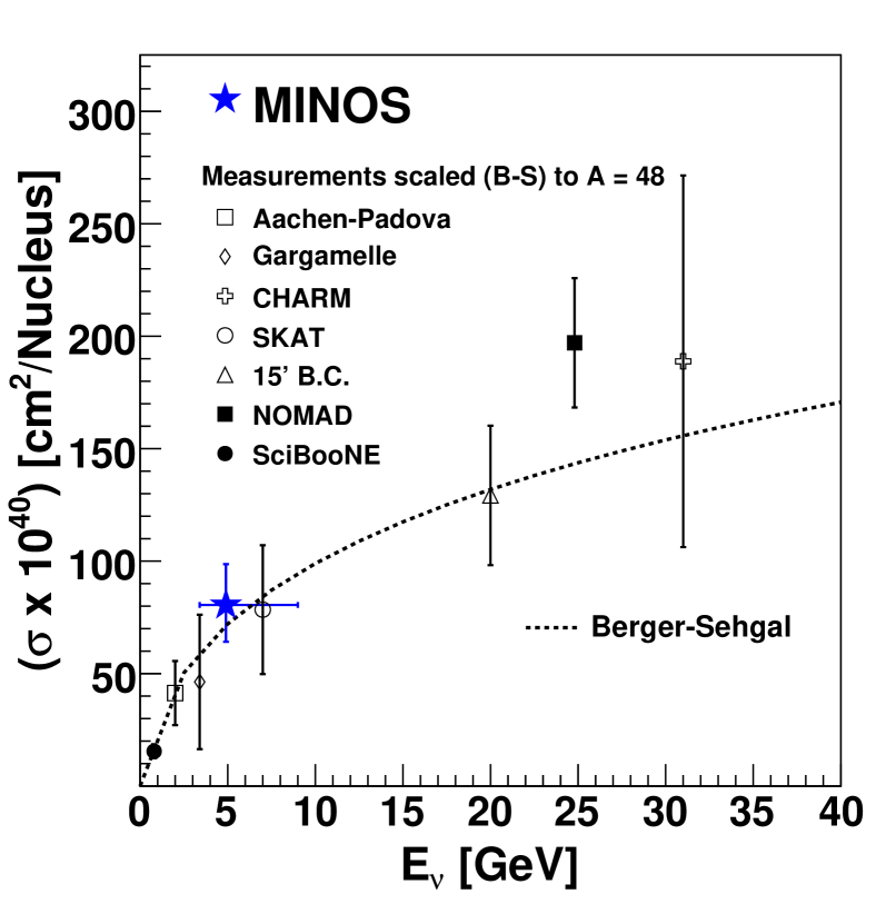
Figure 12: Comparison of the MINOS NC($\uppi^{0}$) coherent scattering total cross section (flux-averaged) to measurements obtained with $\langle E_{\nu}\rangle$ at lower and higher values. Previous measurements are shown scaled to the MINOS target medium, $\langle\mathcal{A}\rangle=48$, for the purpose of comparison. Table 1 compares the previous measurements as reported, to the direct Berger-Sehgal prediction.

XIII Discussion and Conclusion

XIII.1 Cross section versus $E_{\nu}$ and $\mathcal{A}$

As shown by Table 1, the MINOS measurement examines NC($\uppi^{0}$) coherent scattering in an $E_{\nu}$ - $\mathcal{A}$ region that lies outside of the range probed by previous experiments. For the purpose of eliciting the $E_{\nu}$ dependence, the previously reported cross sections (see Table 1) are scaled to an $\mathcal{A}$ = 48 nucleus using the Berger-Sehgal model. (The 15-ft Bubble Chamber and SciBooNE cross section measurements are reported as fractions of the Rein-Sehgal cross sections for neon ref:15BC and for carbon ref:MiniBooNE ; ref:SciBooNE respectively.) The scaled cross-section values are plotted in Fig. 12 together with the $\mathcal{A}$-averaged MINOS measurement (solid star). For purposes of display, the $E_{\nu}$ interval of the measurement is taken to be the interval on either side of 4.9 GeV which includes 34$\%$ of the neutrino flux. Also shown in Fig. 12 is the prediction for $\mathcal{A}$ = 48 of the Berger-Sehgal model (dashed curve). Figures 12 and 13 show that the ensemble of cross-section measurements for Reaction (1), when subjected to “normalization” to common $\langle\mathcal{A}\rangle$ or $\langle E_{\nu}\rangle$, exhibit power-law growth with increasing neutrino energy for fixed $\mathcal{A}$, or with increasing target nucleon number for fixed $\langle E_{\nu}\rangle$.

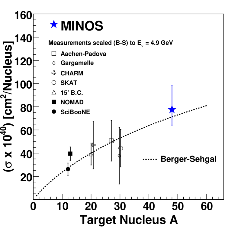
Figure 13: MINOS total cross section (star symbol) for neutrino NC($\uppi^{0}$) coherent scattering at $\langle{E_{\nu}}\rangle$ = 4.9 GeV for nuclei with $\langle\mathcal{A}\rangle=48$. The previous measurements, listed in Table 1, are shown scaled to the same average neutrino energy.

The $\mathcal{A}$-dependence of the coherent cross section is examined by comparing the MINOS result to previous measurements, where the latter are scaled to $\langle E_{\nu}\rangle=4.9$ GeV according to the cross-section ratio predicted by Berger-Sehgal. Figure 13 compares the measurements obtained for the different target $\mathcal{A}$, when their values are scaled in this way. (The extrapolations via Berger-Sehgal to pure iron and carbon targets listed in Table 5 are not plotted.) The high-$\langle\mathcal{A}\rangle$ MINOS result is consistent with the trend predicted by PCAC models ref:Paschos-2009 . In rough terms, the $\mathcal{A}$-dependence in the Berger-Sehgal model for $E_{vis}>1.0$ GeV arises from a convolution of three effects. The coherent nature of the interaction gives an $\mathcal{A}^{2}$ dependence, but that is diminished by the nuclear form factor and by pion absorption. The former falls off as $\exp(-\mathcal{A}^{2/3})$, and the latter as $\exp(-\mathcal{A}^{1/3})$. These effects combine to yield a total cross section with an approximate $\mathcal{A}^{2/3}$ dependence.

XIII.2 Conclusion

The MINOS Near Detector is used to study coherent NC production of single $\uppi^{0}$ mesons initiated by neutrino scattering on a target medium consisting mostly of iron nuclei, with $\langle\mathcal{A}\rangle=48$. Using a low-energy NuMI beam exposure of 2.8$\times 10^{20}$ POT with mean (mode) $E_{\nu}$ of 4.9 GeV (3.0 GeV), a signal sample comprised of 9,550${}^{+1,200}_{-1,590}$ events having final-state $E_{vis}>1.0$ GeV has been isolated. The corresponding flux-averaged, $\mathcal{A}$-averaged partial cross section for events above the analysis $E_{vis}$ threshold of 1.0 GeV is presented in Eq. (11). Extrapolation of the $E_{vis}$ distribution from the analysis 1.0 GeV threshold to zero yields the total coherent scattering cross section. The flux-averaged, $\mathcal{A}$-averaged total cross section is given in Eq. (12). Its value is $\langle\upsigma\rangle=(77.6^{+15.8}_{-17.5})\times 10^{-40}~{}\text{cm}^{2}~{}\text{per nucleus}$. The various neutrino-nucleus NC($\uppi^{0}$) coherent scattering cross sections that are measured or inferred from this work are listed in Table 5. The measurements of coherent scattering Reaction (1) reported here are the first to utilize a target medium of average nucleon number $\langle\mathcal{A}\rangle>30$, and the cross section results of Eqs. (11) and (12) are for coherent scattering at the highest average nucleon number obtained by any experiment to date. Figures 12 and 13 show that these cross sections, as with previous measurements on lighter nuclear media and at lower and higher $\langle{E_{\nu}}\rangle$ values, exhibit the general trends predicted by the Berger-Sehgal coherent scattering model which is founded upon PCAC phenomenology.

XIV Acknowledgments

This work was supported by the US DOE; the UK STFC; the US NSF; the State and University of Minnesota; the University of Athens, Greece; and Brazil’s FAPESP, CNPq, and CAPES. We gratefully acknowledge the staff of Fermilab for invaluable contributions to the research reported here.

Appendix: Fit Validation

Realistic mock data experiments were used to validate the analysis fitting procedure ref:Cherdack-Thesis . The generation of mock data for the latter simulated experiments is more elaborate than for the SSMD experiments. As with SSMD experiments, each mock data sample provides a population of events extending over the $\cos\theta_{shw}$-vs-$E_{vis}$ plane, binned in the same way as for the observed data. However with the full mock data samples, the background templates are adjusted to reflect random fluctuations in each systematic parameter, and the coherent signal content was varied by adjusting the normalization of the signal model over the range $\pm 50\%$. Statistical fluctuations are applied to the event totals in each bin after the templates are combined. The entire background fitting and signal extraction procedure is executed on an ensemble of these mock data samples. Each mock data “experiment” yields a set of best-fit values for the fit parameters, a best-fit $\chi^{2}$, and an acceptance-corrected event rate $N_{fit}$, to be compared to the “true” signal assumed for the simulated experiment, $N_{input}$.

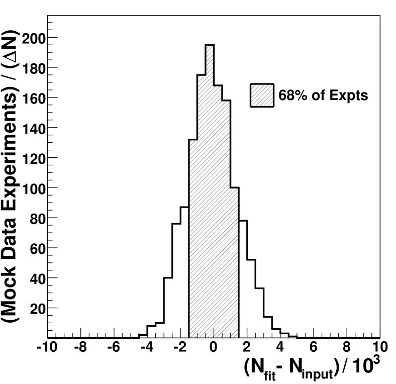
Figure 14: Deviation of best-fit outcomes $N_{fit}$ from coherent signal inputs $N_{input}$, for mock data experiments.

Figure 14 shows the distribution of $N_{fit}-N_{input}$ for an ensemble of mock data experiments. The 1$\upsigma$ width, defined as the region about the peak that includes $68\%$ of the area, was shown to be independent of the input signal normalization. This metric serves as an estimate of the $\pm 1\upsigma$ confidence interval for the final fit procedure, and is measured to be $\pm 15.8\%$. This estimate serves as a cross-check of the uncertainties on the measured signal event rate derived from fitting the data.

References

- (1) E. A. Paschos and D. Schalla, AIP Conf. Proc. 1189, 213 (2009); arXiv:0910.2852.
- (2) M. Hasegawa et al. (K2K Collaboration), Phys. Rev. Lett. 95, 252301 (2005); hep-ex/0506008.
- (3) K. Hiraide et al. (SciBooNE Collaboration), Phys. Rev. D 78, 112004 (2008); arXiv:0811.0369.
- (4) C. T. Kullenberg et al. (NOMAD Collaboration), Phys. Lett. B 682, 177 (2009); arXiv:0910.0062.
- (5) Y. Kurimoto et al. (SciBooNE Collaboration), Phys. Rev. D 81, 033004 (2010); arXiv:0910.5768. Phys. Rev. D 81, 111102(R) (2010); arXiv:1005.0059.
- (6) A. A. Aguilar-Arevalo et al. (MiniBooNE Collaboration), Phys. Lett. B 664, 41 (2008); Phys. Rev. D 81, 013005 (2010); arXiv:0911.2063.
- (7) A. Kartavtsev, E. A. Paschos, and G. J. Gounaris, Phys. Rev. D 74, 054007 (2006); hep-ph/0512139.
- (8) D. Rein and L. M. Sehgal, Phys. Lett. B 657, 207 (2007); hep-ph/0606185.
- (9) Ch. Berger and L. M. Sehgal, Phys. Rev. D 79, 053003 (2009); arXiv:0812.2653.
- (10) E. Hernandez, J. Nieves, and M. J. Vicente Vacas, Phys. Rev. D 80, 013003 (2009); arXiv:0903.5285.
- (11) S. K. Singh, M. Sajjad Athar, and Shakeb Ahmad, Phys. Rev. Lett. 96, 241801 (2006).
- (12) L. Alvarez-Ruso, L. S. Geng, and M. J. Vicente Vacas, Phys. Rev. C 76, 068501 (2007); 80, 029904(E) (2009); arXiv:0707.2172.
- (13) M. Martini, M. Ericson, G. Chanfray, and J. Marteau, Phys. Rev. C 80, 065501 (2009); arXiv:0910.2622.
- (14) J. E. Amaro, E. Hernandez, J. Nieves, and M. Valverde, Phys. Rev. D 79, 013002 (2009); arXiv:0811.1421.
- (15) S. X. Nakamura, T. Sato, T.-S. H. Lee, B. Szczerbinska, and K. Kubodera, Phys. Rev. C 81, 035502 (2010); arXiv:0910.1057.
- (16) E. Hernandez, J. Nieves, and M. Valverde, Phys. Rev. D 82, 077303 (2010); arXiv:1007.3685.
- (17) S. Adler, Phys. Rev. B 135, 963 (1964).
- (18) D. Rein and L. M. Sehgal, Nucl. Phys. B 223, 29 (1983).
- (19) S. Boyd, S. Dytman, E. Hernandez, J. Sobczyk, and R. Tacik, AIP Conf. Proc. 1189, 60 (2009).
- (20) D. G. Michael et al. (MINOS Collaboration), Nucl. Instrum. Methods Phys. Res. Sect. A 596, 190 (2008); arXiv:0805.3170.
- (21) P. Adamson et al. (MINOS Collaboration), Phys. Rev. D 81, 072002 (2010); arXiv:0910.2201.
- (22) C. A. Piketty and L. Stodolsky, Nucl. Phys. B 15, 571 (1970).
- (23) B. Z. Kopeliovich and P. Marage, Int. J. Mod. Phys. A 8, 1513 (1993).
- (24) H. Faissner et al. (Aachen-Padova Collaboration), Phys. Lett. B 125, 230 (1983).
- (25) E. Isiksal, D. Rein, and J. G. Morfin, Phys. Rev. Lett. 52, 1096 (1984).
- (26) H. J. Grabosch et al. (SKAT Collaboration), Z. Phys. C 31, 203 (1986).
- (27) F. Bergsma et al. (CHARM Collaboration), Phys. Lett. B 157, 469 (1985).
- (28) C. Baltay et al. (15’ BC: Columbia-BNL Collaboration), Phys. Rev. Lett. 57, 2629 (1986).
- (29) M. O. Wascko, Acta Phys. Pol. B 40, 2421 (2009); arXiv:0908.1979.
- (30) A. Higuera et al. (MINERvA Collaboration), Phys. Rev. Lett. 113, 261802 (2014); arXiv:1409.3835.
- (31) R. Acciarri et al. (ArgoNeut Collaboration), Phys. Rev. Lett. 113, 261801 (2014); arXiv:1408.0598.
- (32) H. Gallagher, Nucl. Phys. B, Proc. Suppl. 112, 188 (2002).
- (33) P. Adamson et al. (MINOS Collaboration), Phys. Rev. D 91, 012005 (2015).
- (34) T. Hastie, R. Tibshirani, and J. Friedman, The Elements of Statistical Learning, Second Edition, Springer, New York, NY, (2009).
- (35) C.-C. Chang and C.-J. Lin, LIBSVM: a library for support vector machines, 2001, Software available at http://www.csie.ntu.edu.tw/~cjlin/libsvm.
- (36) P. Adamson et al. (MINOS Collaboration), Nucl. Instr. Meth. Phys. Res. A 806, 279 (2016); arXiv:1507.06690.
- (37) P. Adamson et al., (MINOS Collaboration), Phys. Rev. D 77, 072002 (2008); arXiv:0711.0769.
- (38) T. Yang, Ph.D. thesis, Stanford University, 2009, report FERMILAB-THESIS-2009-04.
- (39) J. Boehm, Ph.D. thesis, Harvard University, 2009, report FERMILAB-THESIS-2009-17.
- (40) J. P. Ochoa, Ph.D. thesis, California Institute of Technology, 2009, report FERMILAB-THESIS-2009-44.
- (41) P. L. Vahle, Ph.D. Thesis, University of Texas at Austin, 2004, report FERMILAB-THESIS-2004-35.
- (42) M. A. Kordosky, Ph.D. Thesis, University of Texas at Austin, 2004, report FERMILAB-THESIS-2004-34.
- (43) J. Conrad, M. H. Shaevitz, and T. Bolton, Rev. Mod. Phys. 70, 1341 (1998).
- (44) D. Bhattacharya, Ph.D. thesis, University of Pittsburgh, 2009, report FERMILAB-THESIS-2009-11.
- (45) L. Loiacono, Ph.D. thesis, University of Texas at Austin, 2011, report FERMILAB-THESIS-2011-06.
- (46) J. Wolcott et al. (MINERvA Collaboration), Phys. Rev. Lett. 116, 081802 (2016); arXiv:1509.05729.
- (47) C. Andreopoulos et al., Nucl. Instrum. Methods Phys. Res. Sect. A 614, 87 (2010); arXiv:0905.2517.
- (48) J. Park et al. (MINERvA Collaboration), Phys. Rev. D 93, 112007 (2016); arXiv:1512.07699.
- (49) D. Cherdack, Ph.D. Thesis, Tufts University, 2010, report FERMILAB-THESIS-2010-54.
- (50) R. J. Barlow and C. Beeston, Comput. Phys. Commun. 77, 219 (1993).
- (51) P. Adamson et al. (MINOS Collaboration), Phys. Rev. Lett. 103, 261802 (2009); arXiv:0909.4996.
- (52) M. Martini, M. Ericson, G. Chanfray and J. Marteau, Phys. Rev. C 80, 065501 (2009).
- (53) J. Nieves, I. Ruiz Simo, and M. J. Vicente Vacas, Phys. Lett. B 721, 90 (2013).
- (54) S. Dytman, H. Gallagher, and M. Kordosky, PoS NuFACT08, 041 (2008); arXiv:0806.2119.
- (55) P. Adamson et al., Nucl. Instrum. Methods Phys. Res. Sect. A 556, 119 (2006).
- (56) D. Cherdack, AIP Conf. Proc. 1405, 115 (2011).
- (57) J. Wolcott et al. (MINERvA Collaboration), (MINERvA Collaboration), Phys. Rev. Lett. 117, 111801 (2016); arXiv:1604.01728.
- (58) Program NP based upon B. Z. Kopeliovich, I. Schmidt, and M. Siddikov, Phys. Rev. D 85, 073003 (2012).
- (59) E. A. Paschos and D. Schalla, Phys. Rev. D 80, 033005 (2009); arXiv:0903.0451.