Detecting Vanishing Points using Global Image
Context in a Non-Manhattan World

Abstract

We propose a novel method for detecting horizontal vanishing points and the zenith vanishing point in man-made environments. The dominant trend in existing methods is to first find candidate vanishing points, then remove outliers by enforcing mutual orthogonality. Our method reverses this process: we propose a set of horizon line candidates and score each based on the vanishing points it contains. A key element of our approach is the use of global image context, extracted with a deep convolutional network, to constrain the set of candidates under consideration. Our method does not make a Manhattan-world assumption and can operate effectively on scenes with only a single horizontal vanishing point. We evaluate our approach on three benchmark datasets and achieve state-of-the-art performance on each. In addition, our approach is significantly faster than the previous best method.

1 Introduction

Automatic vanishing point (VP) and horizon line detection are two of the most fundamental problems in geometric computer vision [6, 22]. Knowledge of these quantities is the foundation for many higher level tasks, including image mensuration [10], facade detection [20], geolocalization [4, 31], and camera calibration [2, 12, 15, 17]. Recent work in this area [3, 30, 33] has explored novel problem formulations that significantly increase robustness to noise.

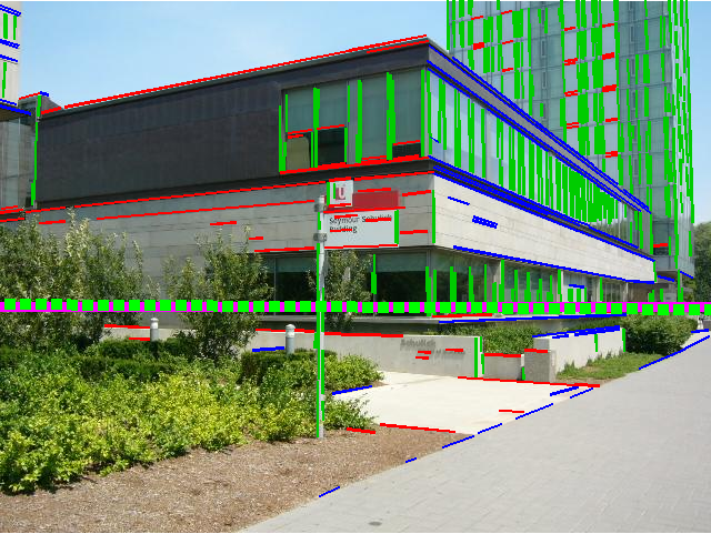
Figure 1: An example result of our method. (left) Horizon line candidates, colored by their scores (red means high score), and the true horizon line (green dash). (right) The horizon line (magenta) estimated by our algorithm is very close to the true horizon line (green dash). Line segments are color coded based on the most consistent detected vanishing point.

A vanishing point results from the intersection of projections of a set of parallel lines in the world. In man-made environments, such sets of lines are often caused by the edges of buildings, roads, and signs. VPs can typically be classified as either vertical, there is one such VP, and horizontal, there are often many such VPs. Given a set of horizontal VPs, there are numerous methods to estimate the horizon line. Therefore, previous approaches to this problem focus on first detecting the vanishing points, which is a challenging problem in many images due to line segment intersections that are not true VPs.

Our approach is to propose candidate horizon lines, score them, and keep the best (Fig. 1). We use a deep convolutional neural network to extract global image context and guide the generation of a set of horizon line candidates. For each candidate, we identify vanishing points by solving a discrete-continuous optimization problem. The final score for each candidate line is based on the consistency of the lines in the image with the selected vanishing points.

This seemingly simple shift in approach leads to the need for novel algorithms and has excellent performance. We evaluated the proposed approach on two standard benchmark datasets, the Eurasian Cities Dataset [5] and the York Urban Dataset [11]. To our knowledge, our approach has the current best performance on both datasets. To evaluate our algorithm further, we also compare with the previous state-of-the-art method (Lezama et al. [19]) on a recently introduced dataset [32]; the results shows that our method is more accurate and much faster.

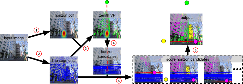
Figure 2: Algorithm overview: 1) use global image context to estimate a prior over horizon lines (Sec. 3); 2) extract line segments; 3) identify the zenith VP (Sec. 4.1); 4) sample horizon line candidates consistent with the zenith VP (Sec. 4.2); 5) find VPs on horizon line candidates (Sec. 4.2); and 6) select the best horizon line based on the VPs it contains (Sec. 4.3).

The main contributions of this work are: 1) a novel method for horizon line/vanishing point detection, which uses global image context to guide precise geometric analysis; 2) a strategy for quickly extracting this context, in the form of constraints on possible horizon lines, using a deep convolutional neural network; 3) a discrete-continuous method for scoring horizon line candidates; and 4) an evaluation of the proposed approach on three benchmark datasets, which highlights that our method is both fast and accurate.

1.1 Related Work

Vanishing points and the horizon line provide a strong characterization of geometric scene structure and as such have been intensely studied for decades [6, 22]. For example, Hoiem et al. [13] show how the horizon line improves the accuracy of object detection. A wide variety of methods have been introduced to estimate these quantities. We provide a brief overview of the main approaches, refer to [26] for a comprehensive review.

Two distinct categories of methods exist, distinguished by the features they use. The first group of methods [5, 9, 11, 25] operate directly on lower-level features, such as edge pixels or image gradients. The second group of methods [1, 11, 19, 21, 28, 30, 33] build on top of the closely related problem of line segment detection. Our work is most closely related to the latter category, so we focus our discussion towards them.

The dominant approach to vanishing point detection from line segments is to cluster the line segments that pass through the same location. Various methods of clustering have been explored, including RANSAC [7], J-linkage [27], and the Hough transform [14]. Once the line segments have been clustered, vanishing points can be estimated using one of many refinement procedures [19, 25, 27, 30, 33].

These procedures typically minimize a nonlinear objective function. An important distinction between such methods is the choice of point and line representation and error metric. Collins and Weiss [8] formulate vanishing point detection as a statistical estimation problem on the Gaussian Sphere, which is similar to the geometry we use. More recent work has explored the use of dual space [19, 35] representations. Among the clustering-based approaches, Xu et al. [33] improve this pipeline by introducing a new point-line consistency function that models errors in the line segment extraction step.

Alternatives to clustering-based approaches have been explored. For example, vanishing point detection from line segments has been modeled as an Uncapacitated Facility Location (UFL) problem [3, 28]. To avoid error accumulation issues encountered by a step-by-step pipeline method, Barinova et al. [5] solve the problem in a unified framework, where edges, lines, and vanishing points fit into a single graphical model.

Our approach is motivated by the fact that properties of the scene, including objects, can provide additional cues for vanishing point and horizon line placement than line segments alone. Unlike existing methods that use J-linkage [27, 33] or similar techniques to find an initial set of VPs by clustering detected lines followed by a refinement step, our approach first proposes candidate horizon lines using global image context.

1.2 Approach Overview

Our approach is motivated by two observations: 1) traditional purely geometric approaches to vanishing point detection often fail in seemingly nonsensical ways and 2) identifying the true vanishing points for many scenes is challenging and computationally expensive due to the large number of outlier line segments. Driven by these observations, we propose a two part strategy. First, we use global image context to estimate priors over the horizon line and the zenith vanishing point (Sec. 3). Using these priors, we introduce a novel VP detection method (Sec. 4) that samples horizon lines from the prior and performs a fast one-dimensional search for high-quality vanishing points in each. Both steps are essential for accurate results: the prior helps ensure a good initialization such that our horizon-first detection method may obtain very precise estimates that are necessary for many scene understanding tasks. See Fig. 2 for an overview of our algorithm.

2 Problem Formulation

The goal of this work is to detect the horizon line, the zenith vanishing point, and any horizontal vanishing points from a single image. The remainder of this section defines the notation and basic geometric facts that we will use throughout. For clarity we use unbolded letters for points in world coordinates or the image plane and bolded letters for points or lines in homogeneous coordinates. We primarily follow the notation convention of Vedaldi and Zisserman [28].

Given a point $(u,v)$ in the image plane, its homogeneous coordinate with respect to the calibrated image plane is denoted by:

$$\mathbf{p}=[\rho(u-c_{u}),\rho(v-c_{v}),1]^{\mathsf{T}}/\Sigma\;,$$

where $\rho$ is a scale constant, $(c_{u},c_{v})$ is the camera principal point in the image frame, which we assume to be the center of the image, and $\Sigma$ is the constant that makes $\mathbf{p}$ a unit vector.

In homogeneous coordinates, both lines and points are represented as three-dimensional vectors (Fig. 3). Computing the line, $\mathbf{l}$, that passes through two points, $(\mathbf{p}_{1},\mathbf{p}_{2})$, and the point, $\mathbf{p}$, at the intersection of two lines, $(\mathbf{l}_{1},\mathbf{l}_{2})$, are defined as follows:

$$\mathbf{l}=\frac{\mathbf{p}_{1}\times\mathbf{p}_{2}}{\|\mathbf{p}_{1}\times\mathbf{p}_{2}\|} \mathbf{p}=\frac{\mathbf{l}_{1}\times\mathbf{l}_{2}}{\|\mathbf{l}_{1}\times\mathbf{l}_{2}\|}\;.$$ (1)

We denote the smallest angle between two vectors $\mathbf{x}$ and $\mathbf{y}$ with $\Theta_{\mathbf{x},\mathbf{y}}=|cos^{-1}(\mathbf{x}^{\mathsf{T}}\mathbf{y})|$. We use this to define the consistency between a line, $\mathbf{l}$, and a point, $\mathbf{p}$, as: $f_{c}(\mathbf{p},\mathbf{l})=\operatorname*{max}(\theta_{con}-\Theta_{\mathbf{p},\mathbf{l}},0)$. The maximum value of consistency between a vanishing point and a line segment is $\theta_{con}$. This will occur if it is possible to extend the line segment to contain the vanishing point.

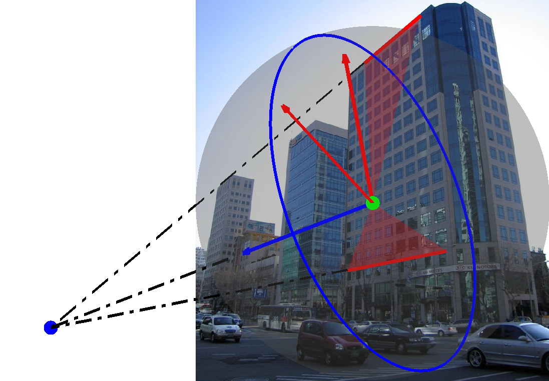
Figure 3: In homogeneous coordinates, lines (red lines) are defined by the normal (red arrow) of the plane (red triangle) they form with the origin (green dot). Two lines form a great circle (blue circle), whose normal (blue arrow) is their common point (blue dot) in homogeneous coordinates.

3 Horizon Priors from Global Image Context

Recent studies show that deep convolutional neural networks (CNNs) are adaptable for a wide variety of tasks [34], and are quite fast in practice. We propose to use a CNN to extract global image context from a single image.

We parameterize the horizon line by its slope angle, $\alpha\in[-\pi,\pi)$, and offset, $o\in[0,\inf)$, which is the shortest distance between the horizon line and the principal point. In order to span the entire horizon line parameter space, we “squash” $o$ from pixel coordinates to the interval $[0,\pi/2)$, through a one-to-one function, $w=tan^{-1}(o/\kappa)$, in which $\kappa$ is a scaling factor that affects how dense the sampling is near the center of the image.

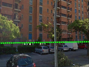
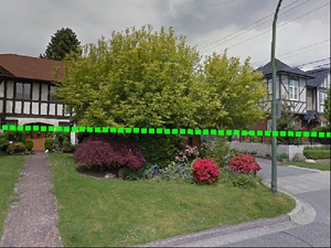
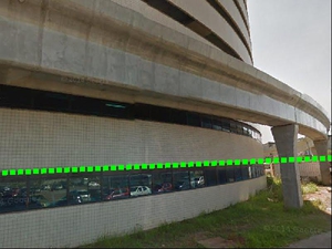
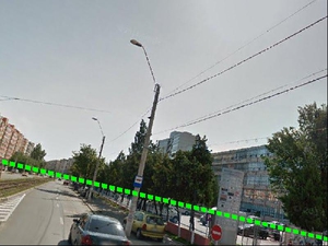
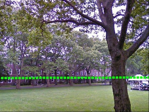
Figure 4: Example images from our training dataset (Sec. 3.2), each overlaid with the ground-truth horizon line.

3.1 Network Architecture

For our task, we adapt the popular AlexNet [18] architecture, which was designed for object recognition as part of the ImageNet ILSVRC-2012 challenge [24]. It consists of five convolutional layers, each followed by a non-linearity (rectified linear unit), and occasionally interspersed with pooling and local response normalization. This is followed by three fully connected layers (referred to as ‘fc6’, ‘fc7’, and ‘fc8’). A softmax is applied to the final output layer to produce a categorical distribution over 1000 object classes. We use this as a foundation to create a CNN that simultaneously generates a categorical distribution for each horizon-line parameter.

We modify the original AlexNet architecture in the following way: The first five convolutional layers are left unmodified. These layers are initialized with weights from a network trained for object detection and scene classification [36]. We remove the original fully connected layers (‘fc6’–‘fc8’) and add two disjoint sets of fully connected layers (‘fc6$\alpha$’–‘fc8$\alpha$’ and ‘fc6$w$’–‘fc8$w$’), one for each target label, $\alpha$ and $w$. We convert the slope, $\alpha$, and the squashed offset, $w$, into independent categorical labels by uniformly dividing their respective domains into 500 bins. We randomly initialize the weights for these new layers.

We train our network using stochastic gradient descent, with a multinomial logistic loss function. The learning rates for the convolutional layers are progressively increased such that the latter layers change more. The new fully connected layers are given full learning rate.

3.2 Training Database

To support training our model of global image context, we construct a large dataset of images with known horizon lines. We make use of equirectangular panoramas downloaded from Google Street View in large metropolitan cities around the world. We identified a set of cities based on population and Street View coverage. From each city, we downloaded panoramas randomly sampled in a $5km\times 5km$ region around the city center. This resulted in $11\,001$ panoramas from 93 cities. Example cities include New York, Rio de Janeiro, London, and Melbourne.

We extracted 10 perspective images from each panorama with randomly sampled horizontal field-of-view (FOV), yaw, pitch, and roll. Here yaw is relative to the Google Street View capture vehicle. We sampled horizontal FOV from a normal distribution with $\mu=60^{\circ}$ and $\sigma=10^{\circ}$. Similarly, pitch and roll are sampled from normal distributions with $\mu=0^{\circ}$ and $\sigma=10^{\circ}$ and $\sigma=5^{\circ}$, respectively. Yaw is sampled uniformly. We truncate these distributions such that horizontal FOV $\in[40^{\circ},80^{\circ}]$, pitch $\in[-30^{\circ},30^{\circ}]$, and roll $\in[-20^{\circ},20^{\circ}]$. These settings were selected empirically to match the distribution of images captured by casual photographers in the wild.

Given the FOV, pitch, and roll of a generated perspective image, it is straightforward to compute the horizon line position in image space. In total, our training database contains $110\,010$ images with known horizon line. Fig. 4 shows several example images from our dataset annotated with the ground-truth horizon line.

3.3 Making the Output Continuous

Given an image, $I$, the network outputs a categorical probability distribution for the slope, $\alpha$, and squashed offset, $w$. We make these distributions continuous by approximating them with a Gaussian distribution. For each, we estimate the mean and variance from $5\,000$ samples generated from the categorical probability distribution. Since the relationship between $w$ and $o$ is one-to-one, this also results in a continuous distribution over $o$. The resulting distributions, $p(\alpha|I)$ and $p(o|I)$, are used in the next step of our approach to aid in detecting the zenith VP and as a prior for sampling candidate horizon lines. To visualize this distribution we observe that the horizon line can be uniquely defined by the point on the line closest to the principal point. Therefore, we can visualize a horizon line distribution as a distribution over points in the image. Fig. 5 shows this distribution for two images.

Figure 5: Global image context imposes a strong prior on horizon line location. The output of our CNN is visualized as an overlaid heatmap, with red indicating more likely locations. For each image, the ground-truth horizon line (dash green) and the line that maximizes the prior (red) are shown.

4 Horizon-First Vanishing Point Detection

We propose an approach to obtain accurate estimates of the horizon line, the zenith vanishing point, and one or more horizontal vanishing points. Given an image, our approach makes use of the distributions estimated from global image context (Sec. 3) and line segments extracted with LSD [29]. The algorithm consists of the following major steps:

1. detect the zenith vanishing point (Sec. 4.1)

2. detect horizontal vanishing points on horizon line candidates (Sec. 4.2)

3. score horizon line candidates with horizontal vanishing points (Sec. 4.3)

The remainder of this section provides details for each of these steps.

4.1 Detecting the Zenith Vanishing Point

To detect the zenith vanishing point, we first select an initial set of line segments using the zenith direction, $\mathbf{l}_{\mathbf{z}}$, from the global image context, then use the RANSAC [7] algorithm to refine it. The zenith direction is the line connecting the principal point and the zenith vanishing point, which is uniquely determined by the horizon line slope (see supplemental material for a proof).

We compute our initial estimate of $\mathbf{l}_{\mathbf{z}}$ using the global image context by choosing the value that maximizes the posterior: $\hat{\alpha}=\operatorname*{arg\,max}_{\alpha}p(\alpha|I)$. To handle the presence of outlier line segments, we first select a set of candidate vertical line segments as the RANSAC inputs by thresholding the angle between each line segment and the estimated zenith direction, $\Theta_{\mathbf{l},\mathbf{l}_{\mathbf{z}}}<\theta_{ver}$. For a randomly sampled pair of line segments with intersection, $\mathbf{p}$, we compute the set of inlier line segments, $\{\mathbf{l}\mid f_{c}(\mathbf{p},\mathbf{l})>0\}$. If the largest set of inliers has a sufficient portion (more than 2% of candidate line segments), we obtain the final estimate of the zenith vanishing point, $\mathbf{z}$, by minimizing the algebraic distance, $\|\mathbf{l}^{\mathsf{T}}\mathbf{p}\|$ using singular value decomposition (SVD), and update the zenith direction, $\mathbf{l}_{\mathbf{z}}$. Otherwise, we keep the zenith direction estimated from the global image context.

4.2 Detecting Horizontal Vanishing Points

We start with sampling a set of horizon line candidates, $\{\mathbf{h}_{i}\}_{1}^{S}$, that are perpendicular to $\mathbf{l}_{\mathbf{z}}$ in the image space, under the distribution of horizon line offsets, $p(o|I)$. See Fig. 6 for examples of horizon line sampling with and without global context.

For each horizon line candidate, we identify a set of horizontal VPs by selecting points along the horizon line where many line segments intersect. We assume that for the true horizon line the identified horizontal VPs will be close to many intersection points and that these intersections will be more tightly clustered than for non-horizon lines. We use this intuition to define a scoring function for horizon line candidates.

As a preprocessing step, given the zenith direction, $\mathbf{l}_{\mathbf{z}}$, and a horizon line candidate, $\mathbf{h}$, we filter out nearly vertical line segments ($\Theta_{\mathbf{l},\mathbf{l}_{\mathbf{z}}}<\theta_{ver}$), which are likely associated with the zenith vanishing point, and nearly horizontal line segments ($\Theta_{\mathbf{l},\mathbf{h}}<\theta_{hor}$), which result in noisy horizon line intersection points. We remove such lines from consideration because they lead to spurious, or uninformative, vanishing points, which decreases accuracy.

Given a horizon line candidate, $\mathbf{h}$, and the filtered line segments in homogeneous coordinates, $\mathcal{L}=\{\mathbf{l}_{i}\}$, we select a set of horizontal VPs, $\mathcal{P}=\{\mathbf{p}_{i}\}$, by minimizing the following objective function:

$$g(\mathcal{P}|\mathbf{h},\mathcal{L}) =-\sum_{\mathbf{p}_{i}\in\mathcal{P}}{\sum_{\mathbf{l}_{j}\in\mathcal{L}}f_{c}(\mathbf{p}_{i},\mathbf{l}_{j})}$$ (2)

subject to:

$$\Theta_{\mathbf{p}_{i},\mathbf{p}_{j}}>\theta_{dist}\;\text{and}\;\left<\mathbf{p}_{i},\mathbf{h}\right>=0,\;\forall(i,j)\;.$$

The constraint prevents two vanishing points from being too close together, which eliminates the possibility of selecting multiple vanishing points in the same location.

We propose the following combinatorial optimization process for obtaining an initial set of vanishing points, followed by a constrained nonlinear optimization to refine the vanishing points.

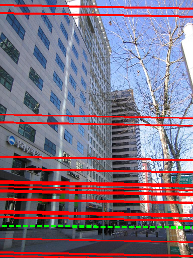
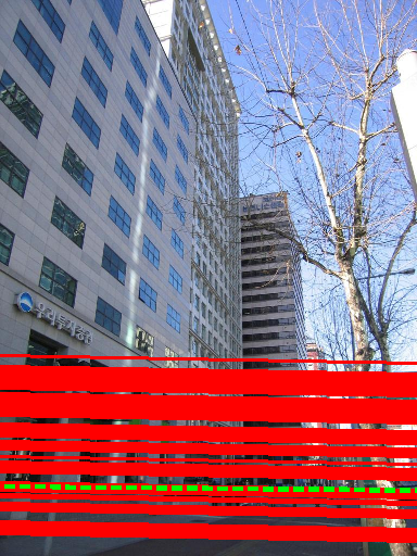
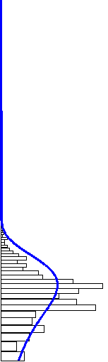
Figure 6: Our method samples more horizon line candidates (red) near the ground truth (green dash) with (middle) global image context than without (left). In the case of sampling with global image context, the offset PDF, $p(o|I)$ (blue curve), is fit from the CNN categorical probability distribution outputs (hollow bins). For clarity, we only show a reduced number of horizon line candidates and bins.

4.2.1 Initialization by Random Sampling and Discrete Optimization

To choose an initial set of candidate vanishing points, $\{\mathbf{p}_{i}\}_{1}^{M}$, we randomly select a subset of line segments, $\{\mathbf{l}_{i}\}_{1}^{M}$, and compute their intersection with the horizon line. We then construct a graph with a node for each vanishing point, $\mathbf{p}_{i}$, each with weight $\sum_{\mathbf{l}_{j}\in\mathcal{L}}f_{c}(\mathbf{p}_{i},\mathbf{l}_{j})$, which is larger if there are many line segments in the image that are consistent with $\mathbf{p}_{i}$. Pairs of nodes, $(i,j)$, are connected if the corresponding vanishing points, $\mathbf{p}_{i},\mathbf{p}_{j}$, are sufficiently close in homogeneous space ($\Theta_{\mathbf{p}_{i},\mathbf{p}_{j}}\leq\theta_{dist}$).

From this randomly sampled set, we select an optimal subset of VPs by maximizing the sum of weights, while ensuring no VPs in the final set are too close. Therefore, the problem of choosing the initial set of VPs reduces to a maximum weighted independent set problem, which is NP-hard in general. Due to the nature of the constraints, the resulting graph has a ring-like structure which means that, in practice, the problem can be quickly solved. Our solver exploits this sparse ring-like structure by finding a set of VPs that when removed convert the ring-like graph into a set of nearly linear sub-graphs (Fig. 7). We solve each subproblem using dynamic programming. The set of VPs with maximum weight, $\{\mathbf{p}_{i}\}_{opt}$, is used as initialization for local refinement. Usually, 2–4 such vanishing points are found near the horizon line ground truth.

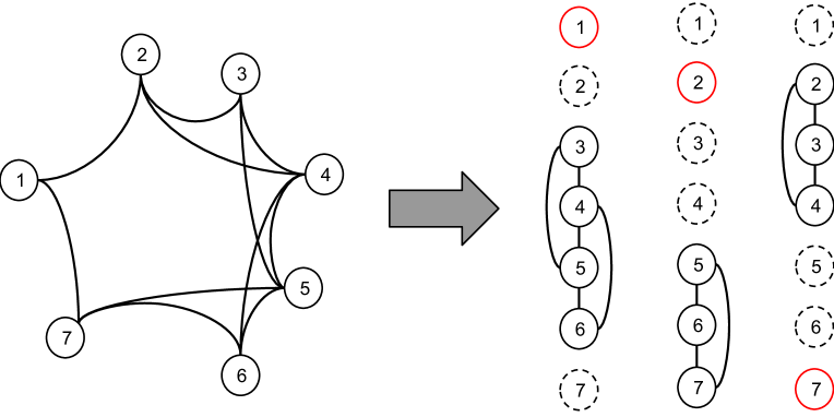
Figure 7: A ring-like graph (left) is converted into three nearly linear subgraphs (right) by partitioning around a node with minimal degree. For the subgraphs, the red node is mandatory, the dashed nodes are excluded, and a subset of the solid nodes are selected using dynamic programming.

4.2.2 Vanishing Points Refinement

Since they were randomly sampled, the set of vanishing points selected during initialization, $\{\mathbf{p}_{i}\}_{opt}$, may not be at the optimal locations. We optimize their locations to further minimize the objective function (2). We perform an EM-like algorithm to refine the vanishing point locations, subject to the constraint that they lie on the horizon line:

• E-step: Given a vanishing point, $\mathbf{p}$, assign line segments that have positive consistency with $\mathbf{p}$: $\{\mathbf{l}|f_{c}(\mathbf{p},\mathbf{l})>0\}$.

• M-step: Given the assigned line segments as a matrix, $\mathbf{L}=[\mathbf{l}_{1},\mathbf{l}_{2},\dots,\mathbf{l}_{n}]$, and the horizon line, $\mathbf{h}$, both represented in homogeneous coordinates, we solve for a refined vanishing point, $\mathbf{p}^{*}$, by minimizing the algebraic distance, $\|\mathbf{L}^{\mathsf{T}}\mathbf{p}\|$ such that $\mathbf{h}^{\mathsf{T}}\mathbf{p}=0$. We define a basis, $\mathbf{B}_{\mathbf{h}}$, for the null space of $\mathbf{h}$, and reformulate the problem as $\mathbf{\lambda}^{*}=\operatorname*{arg\,min}\|\mathbf{L}^{\top}\mathbf{B}_{\mathbf{h}}\mathbf{\lambda}\|$, which we solve using SVD. Given the optimal coefficients, $\mathbf{\lambda}^{*}$, we reconstruct the optimal vanishing point as: $\mathbf{p}^{*}=\frac{\mathbf{B}_{\mathbf{h}}\mathbf{\lambda}^{*}}{\|\mathbf{B}_{\mathbf{h}}\mathbf{\lambda}^{*}\|}$.

We run this refinement iteration until convergence. In practice, this converges quickly; we run at most three iterations for all the experiments. The final set of optimized VPs is then used to assign a score to the current horizon line candidate.

4.3 Optimal Horizon Line Selection

For each horizon line candidate, we assign a score based on the total consistency of lines in the image with the VPs selected in the previous section. The score of a horizon line candidate, $\mathbf{h}$, is defined as:

$$score(\mathbf{h})=\sum_{\{\tilde{\mathbf{p}}_{i}\}}\sum_{\mathbf{l}_{j}\in\mathcal{L}}f_{c}(\tilde{\mathbf{p}}_{i},\mathbf{l}_{j})\;.$$ (3)

To reduce the impact of false positive vanishing points, we select from $\{\mathbf{p}_{i}\}_{opt}$ the two highest weighted vanishing points (or one if $\{\mathbf{p}_{i}\}_{opt}$ contains only one element), $\{\tilde{\mathbf{p}}_{i}\}$, for horizon line scoring.

5 Evaluation

We perform an extensive evaluation of our methods, both quantitatively and qualitatively, on three benchmark datasets. The results show that our method achieves state-of-the-art performance based on horizon-line detection error, the standard criteria in recent work on VP detection [5, 19, 28, 33]. Horizon detection error is defined as the maximum distance from the detected horizon line to the ground-truth horizon line, normalized by the image height. Following tradition, we show the cumulative histogram of these errors and report the area under the curve (AUC).

Our method is implemented using MATLAB, with the exception of detecting line segments, which uses an existing C++ library [29], and extracting global image context, which we implemented using Caffe [16]. We use the parameters defined in Tab. 1 for all experiments. This differs from other methods which usually use different parameters for different datasets.

Table 1: Algorithm parameters (given an $H\times W$ image).

Name	Usage(s)	Value
$\theta_{con}$	Sec. 2	$2^{\circ}$
$\rho$	Sec. 2	$2/\operatorname{max}(H,W)$
$\kappa$	Sec. 3	$1/5\times H$
$\theta_{ver}$	Sec. 4.1, Sec. 4.2	$\Theta_{\mathbf{l},\mathbf{l}_{\mathbf{z}}}<10^{\circ}$
$\theta_{hor}$	Sec. 4.2	$\Theta_{\mathbf{l},\mathbf{h}}<1.5^{\circ}$
$S$	Sec. 4.2	300 candidates
$M$	Sec. 4.2.1	20 line segments
$\theta_{dist}$	Sec. 4.2, Sec. 4.2.1	$\Theta_{\mathbf{p}_{i},\mathbf{p}_{j}}>33^{\circ}$

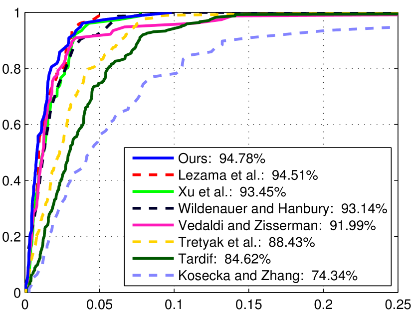
(a) YUD

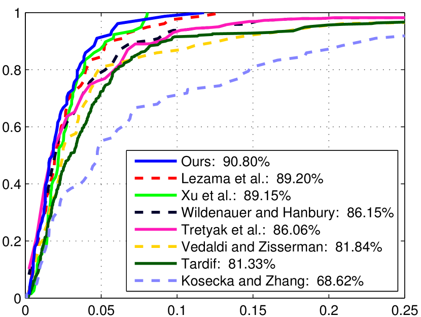
(b) ECD

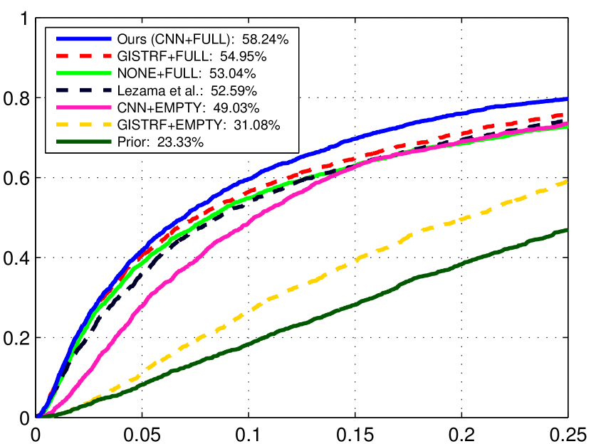
(c) HLW

Figure 8: For three benchmark datasets, the fraction of images (y-axis) with a horizon error less than a threshold (x-axis). The AUC for each curve is shown in the legend. For additional details see Sec. 5.

5.1 Quantitative Evaluation

The York Urban Dataset (YUD) [11] is a commonly used dataset for evaluating horizon line estimation methods. It contains 102 images and ground-truth vanishing points. The scenes obey the Manhattan-world assumption, however we do not take advantage of this assumption. Fig. 8(a) shows the performance of our methods relative to previous work on YUD. These results demonstrate that our method achieves state-of-the-art AUC, improving upon the previous best of Lezama et al. [19] by 0.28%, a relative improvement of 5%. This is especially impressive given that our method only requires an average of 1 second per image, while Lezama et al. requires approximately 30 seconds per image.

The Eurasian Cities Dataset (ECD) [5] is another commonly used benchmark dataset, which is considered challenging due to the large number of outlier line segments and complex scene geometries. It contains 103 images captured in urban areas and, unlike the YUD dataset, not all images satisfy the Manhattan-world assumption. It provides reliable horizon line ground truth and is widely considered difficult for horizon line detection. To our knowledge, the previous state-of-the-art performance in terms of the AUC metric on this dataset was achieved by Lezama et al. [19]. Our algorithm improves upon their performance, increasing the state of the art to 90.8%. This is a significant relative improvement of 14.8%, especially considering their improvement relative to the state of the art was 0.5%. On ECD, our method takes an average of 3 seconds per image, while Lezama et al. requires approximately 60 seconds per image. We present the performance comparison with other methods in Fig. 8(b).

The Horizon Lines in the Wild (HLW) dataset [32] is a new, very challenging benchmark dataset. We use the provided test set, which contains approximately $2\,000$ images from diverse locations, with many images not adhering to the Manhattan-world assumption. Fig. 8(c) compares our method with the method of Lezama et al. [19] (the only publicly available implementation from a recent method). Our method is significantly better, achieving 58.24% versus 52.59% AUC.

Table 2: Component error analysis (AUC).

Method	YUD	ECD	HLW
Lezama et al. [19]	94.51%	89.20%	52.59%
NONE+FULL	93.87%	87.94%	53.04%
GISTRF+EMPTY	53.36%	32.69%	31.08%
GISTRF+FULL	94.66%	87.60%	54.95%
CNN+EMPTY	73.67%	67.64%	49.03%
CNN+FULL (Ours)	94.78%	90.80%	58.24%

5.2 Component Error Analysis

Our method consists of two major components: global context extraction (Sec. 3) and horizon-first vanishing point detection (Sec. 4). This section provides an analysis of the impact each component has on accuracy.

To evaluate the impact of global context extraction, we considered three alternatives: our proposed approach (CNN), replacing the CNN with a random forest (using the Python “sklearn” library with 25 trees) applied to a GIST [23] descriptor (GISTRF), and omitting context entirely (NONE). When omitting the global context, we assume no camera roll (horizon lines are horizontal in the image) and sample horizon lines uniformly between $[-2H,2H]$ ($H$ is the image height). To evaluate the impact of vanishing point detection, we considered two alternatives: our proposed approach (FULL) and omitting the vanishing point detection step (EMPTY). When omitting vanishing point detection, we directly estimate the horizon line, $(\alpha,o)$, by maximizing the posterior estimated by our global-context CNN, $p(\alpha,o|I)$.

Quantitative results presented in Tab. 2 show that both components play important roles in the algorithm and that CNN provides better global context information than GISTRF. Though our vanishing point detection performs well by itself (see column NONE+FULL), global image context helps improve the accuracy further. Fig. 8(c) visualizes these results as a cumulative histogram of horizon error on HLW. To illustrate the impact of global image context, we present two examples in Fig. 9 that compare horizon line estimates obtained using global context (CNN+FULL) and without (NONE+FULL). When using global context, the estimated horizon lines are very close to the ground truth. Without, the estimates obtained are implausible, even resulting in an estimate that is off the image.

Figure 9: Two images where horizon line estimates are much better with global context (left) than without (right).

Figure 10: Example results produced by our method. (rows 1 and 3) Line segments color coded based on the most consistent VP, the ground-truth (green dash), and detected horizon lines (magenta). For clarity only the top two horizontal VPs are shown. (rows 2 and 4) The line segments (dots) and their VPs (rings) represented in homogeneous coordinates. (last column) Two failure cases of our method, caused by irregularly shaped objects (bottom) and short edges (top).

5.3 Failure Cases

We highlight two representative failure cases in the last column of Fig. 10. The top image fails due to the propagation of measurement errors from the short line segments. The bottom image is challenging because the curved structures lead to indistinct VPs. Despite this, global context helps our method produce plausible results, while other methods (e.g., [5]) fail dramatically.

6 Conclusion

We presented a novel vanishing point detection algorithm that obtains state-of-the-art performance on three benchmark datasets. The main innovation in our method is the use of global image context to sample possible horizon lines, followed by a novel discrete-continuous procedure to score each horizon line by choosing the optimal vanishing points for the line. Our method is both more accurate and more efficient than the previous state-of-the-art algorithm, requiring no parameter tuning for a new testing dataset, which is common in other methods.

References

- [1] A. Almansa, A. Desolneux, and S. Vamech. Vanishing point detection without any a priori information. PAMI, 25(4):502–507, 2003.
- [2] M. E. Antone and S. Teller. Automatic recovery of relative camera rotations for urban scenes. In CVPR, 2000.
- [3] M. Antunes and J. P. Barreto. A global approach for the detection of vanishing points and mutually orthogonal vanishing directions. In CVPR, 2013.
- [4] G. Baatz, K. Köser, D. Chen, R. Grzeszczuk, and M. Pollefeys. Handling urban location recognition as a 2d homothetic problem. In ECCV, 2010.
- [5] O. Barinova, V. Lempitsky, E. Tretiak, and P. Kohli. Geometric image parsing in man-made environments. In ECCV, 2010.
- [6] S. T. Barnard. Interpreting perspective images. Artificial intelligence, 21(4):435–462, 1983.
- [7] R. C. Bolles and M. A. Fischler. A ransac-based approach to model fitting and its application to finding cylinders in range data. In International Joint Conference on Artificial Intelligence, 1981.
- [8] R. T. Collins and R. S. Weiss. Vanishing point calculation as a statistical inference on the unit sphere. In ICCV, 1990.
- [9] J. M. Coughlan and A. L. Yuille. Manhattan world: Compass direction from a single image by bayesian inference. In ICCV, 1999.
- [10] A. Criminisi, I. Reid, and A. Zisserman. Single view metrology. IJCV, 40(2):123–148, 2000.
- [11] P. Denis, J. H. Elder, and F. J. Estrada. Efficient edge-based methods for estimating manhattan frames in urban imagery. In ECCV, 2008.
- [12] L. Grammatikopoulos, G. Karras, and E. Petsa. An automatic approach for camera calibration from vanishing points. ISPRS Journal of Photogrammetry and Remote Sensing, 62(1):64–76, 2007.
- [13] D. Hoiem, A. A. Efros, and M. Hebert. Putting objects in perspective. IJCV, 80(1):3–15, 2008.
- [14] P. V. Hough. Machine analysis of bubble chamber pictures. In International Conference on High Energy Accelerators and Instrumentation, volume 73, 1959.
- [15] N. Jacobs, M. Islam, and S. Workman. Cloud Motion as a Calibration Cue. In CVPR, 2013.
- [16] Y. Jia, E. Shelhamer, J. Donahue, S. Karayev, J. Long, R. Girshick, S. Guadarrama, and T. Darrell. Caffe: Convolutional architecture for fast feature embedding. arXiv preprint arXiv:1408.5093, 2014.
- [17] J. Košecká and W. Zhang. Video compass. In ECCV, 2002.
- [18] A. Krizhevsky, I. Sutskever, and G. E. Hinton. Imagenet classification with deep convolutional neural networks. In NIPS, 2012.
- [19] J. Lezama, R. G. v. Gioi, G. Randall, and J.-M. Morel. Finding vanishing points via point alignments in image primal and dual domains. In CVPR, 2014.
- [20] J. Liu and Y. Liu. Local regularity-driven city-scale facade detection from aerial images. In CVPR, 2014.
- [21] E. Lutton, H. Maitre, and J. Lopez-Krahe. Contribution to the determination of vanishing points using hough transform. PAMI, 16(4):430–438, 1994.
- [22] M. J. Magee and J. K. Aggarwal. Determining vanishing points from perspective images. Computer Vision, Graphics, and Image Processing, 26(2):256–267, 1984.
- [23] A. Oliva and A. Torralba. Modeling the shape of the scene: A holistic representation of the spatial envelope. IJCV, 42(3):145–175, 2001.
- [24] O. Russakovsky, J. Deng, H. Su, J. Krause, S. Satheesh, S. Ma, Z. Huang, A. Karpathy, A. Khosla, M. Bernstein, A. C. Berg, and L. Fei-Fei. Imagenet large scale visual recognition challenge. IJCV, 2015.
- [25] G. Schindler and F. Dellaert. Atlanta world: An expectation maximization framework for simultaneous low-level edge grouping and camera calibration in complex man-made environments. In CVPR, 2004.
- [26] R. Szeliski. Computer vision: algorithms and applications. Springer, 2010.
- [27] J.-P. Tardif. Non-iterative approach for fast and accurate vanishing point detection. In ICCV, 2009.
- [28] A. Vedaldi and A. Zisserman. Self-similar sketch. In ECCV, 2012.
- [29] R. G. Von Gioi, J. Jakubowicz, J.-M. Morel, and G. Randall. Lsd: A fast line segment detector with a false detection control. PAMI, 32(4):722–732, 2010.
- [30] H. Wildenauer and A. Hanbury. Robust camera self-calibration from monocular images of manhattan worlds. In CVPR, 2012.
- [31] S. Workman, R. P. Mihail, and N. Jacobs. A Pot of Gold: Rainbows as a Calibration Cue. In ECCV, 2014.
- [32] S. Workman, M. Zhai, and N. Jacobs. Horizon lines in the wild. arXiv preprint arXiv:1604.02129, 2016.
- [33] Y. Xu, S. Oh, and A. Hoogs. A minimum error vanishing point detection approach for uncalibrated monocular images of man-made environments. In CVPR, 2013.
- [34] J. Yosinski, J. Clune, Y. Bengio, and H. Lipson. How transferable are features in deep neural networks? In NIPS, 2014.
- [35] Y.-G. Zhao, X. Wang, L.-B. Feng, G. Chen, T.-P. Wu, and C.-K. Tang. Calculating vanishing points in dual space. Intelligent Science and Intelligent Data Engineering, pages 522–530, 2013.
- [36] B. Zhou, A. Lapedriza, J. Xiao, A. Torralba, and A. Oliva. Learning Deep Features for Scene Recognition using Places Database. In NIPS, 2014.