Finite temperature corrections to a NLO Nambu-Jona-Lasinio model ^∗

Abstract

We derive the next-to-leading order correction to the Nambu-Jona-Lasinio model starting from quantum chromodynamics. So, we are able to fix the constants of the Nambu-Jona-Lasinio model from quantum chromodynamics and analyze the behavior of strong interactions at low energies. The technique is to expand in powers of currents the generating functional. We apply it to a simple Yukawa model with self-interaction showing how this has a Nambu-Jona-Lasinio model and its higher order corrections as a low-energy limit. The same is shown to happen for quantum chromodynamics in the chiral limit with two quarks. We prove that a consistent thermodynamic behaviour is obtained as expected for the given parameters.

Recent lattice studies for the gluon propagator [1, 2, 3] and the spectrum [4, 5] showed evidence of a mass gap in a Yang-Mills theory without fermionic degrees of freedom. These results received theoretical support [6, 7, 8, 9, 10, 11, 12] providing a closed form formula for the gluon propagator. An understanding of the gluon propagator is pivotal to derive the low-energy behaviour of QCD in a manageable effective theory. Some other results are also essential for this aim as the behaviour of the running coupling in the infared limit [13, 14, 15, 16, 17, 18, 19] (see also the review [20]) beside the gluon propagator. We will see that, for the latter, the instanton liquid plays an essential role [21, 22].

We have succeeded to show that a non-local Nambu-Jona-Lasinio model (nlNJL) represents the low energy limit of QCD [23, 24, 25, 26, 27]. Here we generalizes this approach to get higher order corrections to the nlNJL verifying its consistency in a fully thermodynamic computation. This gives strong support to the already postulated extensions to the NJL model [28, 29, 30, 31, 32]. As a historical aside, we show how the well-known Yukawa model recovers a nlNJL model. This was already shown in [33] and does justice a posteriori to Yukawa’s great insight.

So, in order to understand the technique, we consider the simplest Yukawa model: A scalar field interacting with a quark field. One has

$$L_{Y}=\bar{q}(i\not{\partial}-g\phi)q+\frac{1}{2}(\partial\phi)^{2}-\frac{\lambda}{4}\phi^{4}.$$ (1)

Then, the generating functional is

$$Z_{Y}[\bar{\eta},\eta]\!\!\!\! = \!\!\!\!\int[d\bar{q}][dq]\exp\left[-i\int d^{4}x\bar{q}\left(i\not{\partial}-g\frac{\delta}{i\delta j}\right)q\right]\times\qquad$$ (2)

$$\left.\exp(iW[j])\right|_{j=0}\exp\left[i\int d^{4}x\left(\bar{\eta}q+\bar{q}\eta\right)\right]$$

being

$$W[j]\!\!\!\! = \!\!\!\!W[0]+\int d^{4}xj(x)\phi_{0}(x)$$

$$+ \!\!\!\!\frac{1}{2}\int d^{4}xd^{4}x_{1}j(x)\Delta(x-x_{1})j(x_{1})+O(j^{3}).$$

We have supposed to have exactly solved for the equation of motion of the scalar field obtaining the 1- and 2-point functions written as $\phi_{0}(x)$ and $\Delta(x-x_{1})$ [34, 35]. The idea behind the functional ( Finite temperature corrections to a NLO Nambu-Jona-Lasinio model ^∗) is a current expansion already devised in the ’80 [36]. The 1-point function is given by

$$\phi_{0}(x)=\mu\left(2/\lambda\right)^{\frac{1}{4}}{\rm sn}(p\cdot x+\theta,-1)$$ (4)

being sn the snoidal Jacobi function, $\mu$ and $\theta$ arbitrary integration constants. The 2-point function is

$$\Delta(p)=\sum_{n=0}^{\infty}\frac{B_{n}}{p^{2}-m_{n}^{2}+i\epsilon}$$ (5)

with

$$B_{n}=(2n+1)^{2}\frac{\pi^{3}}{4K^{3}(-1)}\frac{e^{-(n+\frac{1}{2})\pi}}{1+e^{-(2n+1)\pi}}.$$ (6)

A mass spectrum is obtained given by

$$m_{n}=(2n+1)(\pi/2K(-1))\left(\lambda/2\right)^{\frac{1}{4}}\mu$$ (7)

and $K(-1)\approx 1.3111028777$ is an elliptic integral. We can see that the action for the quark field, after the introduction of the n-point functions, recovers a nlNJL model and its possible higher order corrections

$$S_{q}\!\!\!\! = \!\!\!\!\int d^{4}x\bar{q}\left(i\not{\partial}-g\phi_{0}(x)\right.$$ (8)

$$- \!\!\!\!\left.\frac{g^{2}}{2}\int d^{4}x^{\prime}\Delta(x-x^{\prime})\bar{q}q\right)q+\ldots,$$

where dots imply higher powers of the quark current. If we average on the phase of the background field $\phi_{0}$, that is arbitrary, and fix this constant to zero, we are left with

$$S_{NJL}\!\!\!\! = \!\!\!\!\int d^{4}x\left[\bar{q}(x)i{\not{\partial}}q(x)\right.$$

$$- \!\!\!\!\left.\frac{g^{2}}{2}\int d^{4}x^{\prime}\Delta(x-x^{\prime})\bar{q}(x)q(x)\bar{q}(x^{\prime})q(x^{\prime})\right].$$

We note that, in the low-energy (local) limit $\Delta(x-x^{\prime})=-(C_{0}/m_{0}^{2})\delta^{4}(x-x^{\prime})$, that leaves

$$S_{NJL}\!\!\!\! = \!\!\!\!\int d^{4}x\left[\bar{q}(x)i{\not{\partial}}q(x)\right.$$ (10)

$$+ \!\!\!\!\left.C_{0}\frac{g^{2}}{2m_{0}^{2}}\bar{q}(x)q(x)\bar{q}(x)q(x)\right]$$

and the NJL constant $G=C_{0}g^{2}/m_{0}^{2}$ is fixed by the original Yukawa Lagrangian that describes the microscopic dynamics of the model.

Yang-Mills theory admits a set of exact solutions and all the correlation functions can be obtained [37]. Indeed, such solutions map on scalar field solutions [12]. This means that the following functional series holds in this case

$$W_{YM}[j,\epsilon,\bar{\epsilon}]\!\!\!\! = \!\!\!\!\int d^{4}x\bar{\epsilon}(x)G(x)\epsilon(x)+\int d^{4}x\Phi_{\mu}^{a}(x)j^{\mu a}(x)$$ (11)

$$- \!\!\!\!\int d^{4}x_{1}d^{4}x_{2}j^{\mu a}(x_{1})\Delta_{\mu\nu}^{ab}(x_{1}-x_{2})j^{\nu b}(x_{2})$$

$$+ \!\!\!\!\int d^{4}xd^{4}x_{1}d^{4}x_{2}d^{4}x_{3}\Phi^{\mu a}(x)\Delta_{\mu\nu}^{ab}(x-x_{1})j^{\nu b}(x_{1})\times$$

$$\Delta_{\kappa\lambda}^{cd}(x-x_{2})j^{\kappa c}(x_{2})\Delta^{\lambda de}_{\rho}(x-x_{3})j^{\rho e}(x_{3})$$

$$+ \!\!\!\!\int d^{4}xd^{4}x_{1}d^{4}x_{2}d^{4}x_{3}d^{4}x_{4}\Delta_{\mu\nu}^{ab}(x-x_{1})j^{\mu a}(x_{1})\times$$

$$\Delta_{\lambda}^{\nu bc}(x-x_{2})j^{\lambda c}(x_{2})\times$$

$$\Delta^{de}_{\kappa\rho}(x-x_{3})j^{\kappa d}(x_{3})\times$$

$$\Delta^{\rho ef}_{\theta}(x-x_{4})j^{\theta f}(x_{4})+O(j^{5}).$$

Here $G(x)$ is the ghost two-point function, $\Phi^{\mu a}(x)$ is the Yang-Mills 1-point function and $\Delta_{\mu\nu}^{ab}(x_{1}-x_{2})$ the Yang-Mills 2-point function. Using the substitution with quark currents $j^{\mu a}(x_{1})\rightarrow\sum_{q}\bar{q}(x)\frac{\lambda^{a}}{2}\gamma^{\mu}q(x)$ we get a nlNJL model from QCD at low-energies

$$S_{NJL}\!\!\!\! = \!\!\!\!-g\int d^{4}x\Phi_{\mu}^{a}(x)\sum_{q}\bar{q}(x)\frac{\lambda^{a}}{2}\gamma^{\mu}q(x)$$ (12)

$$- \!\!\!\!g^{2}\int d^{4}x_{1}d^{4}x_{2}\sum_{q}\bar{q}(x_{1})\frac{\lambda^{a}}{2}\gamma^{\mu}q(x_{1})\Delta(x_{1}-x_{2})\times$$

$$\sum_{q^{\prime}}\bar{q}^{\prime}(x_{2})\frac{\lambda^{a}}{2}\gamma_{\mu}q^{\prime}(x_{2})$$

$$- \!\!\!\!g^{3}\int d^{4}xd^{4}x_{1}d^{4}x_{2}d^{4}x_{3}\Phi^{\mu a}(x)\Delta(x-x_{1})\times$$

$$\sum_{q}\bar{q}(x_{1})\frac{\lambda^{a}}{2}\gamma_{\mu}q(x_{1})\times$$

$$\Delta(x-x_{2})\sum_{q^{\prime}}\bar{q}^{\prime}(x_{2})\frac{\lambda^{b}}{2}\gamma^{\nu}q^{\prime}(x_{2})\Delta(x-x_{3})\times$$

$$\sum_{q^{\prime\prime}}\bar{q}^{\prime\prime}(x_{3})\frac{\lambda^{b}}{2}\gamma_{\nu}q^{\prime\prime}(x_{3})$$

$$+ \!\!\!\!g^{4}\int d^{4}xd^{4}x_{1}d^{4}x_{2}d^{4}x_{3}d^{4}x_{4}\Delta(x-x_{1})\times$$

$$\sum_{q}\bar{q}(x_{1})\frac{\lambda^{a}}{2}\gamma^{\mu}q(x_{1})\times$$

$$\Delta(x-x_{2})\sum_{q^{\prime}}\bar{q}^{\prime}(x_{2})\frac{\lambda^{a}}{2}\gamma_{\mu}q^{\prime}(x_{2})\times$$

$$\Delta(x-x_{3})\sum_{q^{\prime\prime}}\bar{q}^{\prime\prime}(x_{3})\frac{\lambda^{b}}{2}\gamma^{\nu}q^{\prime\prime}(x_{3})\times$$

$$\Delta(x-x_{4})\sum_{q^{\prime\prime\prime}}\bar{q}^{\prime\prime\prime}(x_{4})\frac{\lambda^{b}}{2}\gamma_{\nu}q^{\prime\prime\prime}(x_{4}).$$

For the non-local limit the propagator yields

$${\cal G}(p)\!\!\!\! = \!\!\!\!-\frac{1}{2}g^{2}\Delta(p)$$

$$= \!\!\!\!-\frac{1}{2}g^{2}\sum_{n=0}^{\infty}\frac{B_{n}}{p^{2}-(2n+1)^{2}(\pi/2K(i))^{2}\tilde{\sigma}+i\epsilon}=\frac{G}{2}{\cal C}(p)$$

to be compared with [21] for instanton liquid at $\sqrt{\sigma}=0.417\ GeV$ and $d^{-1}=0.58\ GeV$

$$\mathcal{C}_{I}(\xi)=4\pi^{2}d^{2}\left\{\xi\frac{d}{d\xi}\big{[}I_{0}(\xi)K_{0}(\xi)-I_{1}(\xi)K_{1}(\xi)\big{]}\right\}^{2}$$ (14)

with $\xi=\frac{|p|d}{2}$. The comparison is given in fig. 1 and we get a strikingly good agreement.

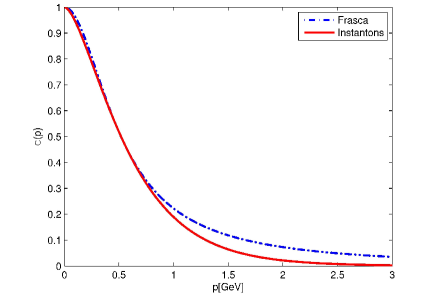
Figure 1: Comparison of eq.( Finite temperature corrections to a NLO Nambu-Jona-Lasinio model ^∗) with the one of an instanton liquid given in Ref [21].

From the nlNJL model we take the local limit and two-flavor approximation that are enough for our aims. So, for $\psi=(u,d)$ and averaging on the phase of $\Phi^{\mu a}(x)$ as already done for the Yukawa model, we get

$$W_{NJL}[q,\bar{q}]\!\!\!\! = \!\!\!\!\frac{G}{2}\int d^{4}x\left[\bar{\psi}(x)\gamma^{\mu}\psi(x)\bar{\psi}(x)\gamma_{\mu}\psi(x)\right.$$ (15)

$$+ \!\!\!\!\left.\bar{\psi}(x)\gamma^{\mu}{\bm{\tau}}\psi(x)\bar{\psi}(x)\gamma_{\mu}{\bm{\tau}}\psi(x)\right]$$

$$+ \!\!\!\!G_{8}\int d^{4}x\left[\bar{\psi}(x)\gamma^{\mu}\psi(x)\bar{\psi}(x)\gamma_{\mu}\psi(x)\right.$$

$$+ \!\!\!\!\left.\bar{\psi}(x)\gamma^{\mu}{\bm{\tau}}\psi(x)\bar{\psi}(x)\gamma_{\mu}{\bm{\tau}}\psi(x)\right]\times$$

$$\left[\bar{\psi}(x)\gamma^{\mu}\psi(x)\bar{\psi}(x)\gamma_{\mu}\psi(x)\right.$$

$$+ \!\!\!\!\left.\bar{\psi}(x)\gamma^{\mu}{\bm{\tau}}\psi(x)\bar{\psi}(x)\gamma_{\mu}{\bm{\tau}}\psi(x)\right]$$

with $G$ the usual NJL coupling given by eq.( Finite temperature corrections to a NLO Nambu-Jona-Lasinio model ^∗) and we have

$$G_{8}\!\!\!\! = \!\!\!\!4g^{-4}\left[{\cal G}(0)\right]^{4}=\frac{g^{4}}{4(\pi/2K(-1))^{8}{\tilde{\sigma}}^{4}}\left[\sum_{n=0}^{\infty}\frac{B_{n}}{(2n+1)^{2}}\right]^{4}$$ (16)

$$\approx \!\!\!\!0.096\frac{g^{4}}{{\tilde{\sigma}}^{4}}.$$

This shows that the next-to-leading order correction to the NJL model is an eight quark interaction term in agreement with what recently postulated [28, 29, 30, 31, 32]. The question we want to answer is if such a term we derived from QCD is consistent with the expected thermodynamic behaviour of the theory. We are going to discuss this point below.

To get an understanding of this model we have to analyze the gap equation. We have to solve the self-consistent set of equations [30], in the chiral limit $m_{u}=m_{d}=0$,

$$M+Gh+\frac{3}{16}G_{8}h^{3}\!\!\!\! = \!\!\!\!0$$

$$h(M)+\frac{NN_{f}}{2\pi^{2}}MJ_{0}(M^{2})\!\!\!\! = \!\!\!\!0.$$ (17)

where $J_{0}(M^{2})$ is the first of NJL integrals and is yielded, at zero temperature and chemical potential, by

$$J_{0}(M^{2})\!\!\!\! = \!\!\!\!16\pi^{2}i\int_{\Lambda}\frac{d^{4}p}{(2\pi)^{4}}\frac{1}{p^{2}-M^{2}}$$ (18)

$$= \!\!\!\!\Lambda^{2}-M^{2}\ln\left(1+\frac{M^{2}}{\Lambda^{2}}\right).$$

A cut-off $\Lambda$ is needed to regularize the theory. We get $M_{eff}=0.63\ GeV$ for the quark effective mass with a cut-off $\Lambda=0.747\ GeV$, assuming $G\approx 9.37\ GeV^{-2}$ (see [26]) and $G_{8}=G^{4}/(\sqrt{2}g)^{4}$.

At finite temperature and chemical potential one has for the gap equation

$$h(M)+\frac{NN_{f}}{2\pi^{2}}MJ_{0}(M^{2},T,\mu)=0.$$ (19)

with

$$J_{0}(M^{2},T,\mu)\!\!\!\! = \!\!\!\!J_{0}(M^{2})-4\int_{0}^{\Lambda}dp\frac{p^{2}}{E_{p}}\times$$ (20)

$$\left(\frac{1}{1+e^{\beta(E_{p}-\mu)}}+\frac{1}{1+e^{\beta(E_{p}+\mu)}}\right)$$

being $E_{p}=\sqrt{p^{2}+M^{2}}$. We can treat this integral numerically to obtain the phase diagram in this case. But we note a simple fact, already at this stage, in the chiral limit $M\rightarrow 0$ the critical temperature is left untouched by the eight quark term. This can be understood by noticing that

$$\lim_{M\rightarrow 0}\frac{h(M)}{M}=-\frac{1}{G}$$ (21)

leaving us with the usual gap equation to determine the critical temperature [38, 27]. Fig. 2 presents the quark condensate $M_{q}(T,\mu)=-G\langle\bar{q}q\rangle$ and the critical line $T_{c}=T_{c}(\mu)$ at $M_{q}(T_{c},\mu)=0$ with the given parameters

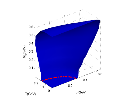
Figure 2: Effective quark mass as a function of $\mu$ and $T$. The critical line $T_{c}=T_{c}(\mu)$ is plotted in dot-dashed red.

We have shown how to derive a nlNJL model starting from a Yukawa theory. Recent studies permit to obtain the NJL model directly from QCD in the low-energy limit with the same technique. We have found the next-to-leading order correction to the NJL model yielding and 8-quark interaction term as already postulated in literature. The critical temperature, in the chiral limit setting quark masses to zero, is unaffected by this correction. A consistent thermodynamic behaviour is also obtained as expected for the given parameters, particularly, we recover a consistent curve for the critical temperature as a function of the chemical potential. Further studies will be needed to understand the physical spectrum of the theory in the low-energy limit. In this respect, it is worthwhile to point out that a non-confining theory, as NJL is, yields just bound states and no free quarks. Low-energy physical states cannot coincide with those in the ultraviolet limit.

I have to thank Silvio Sorella for several enlightening discussions during the Conference.

References

• [1] I. L. Bogolubsky, E. M. Ilgenfritz, M. Muller-Preussker, A. Sternbeck, PoS LAT2007, 290 (2007).
• [2] A. Cucchieri, T. Mendes, PoS LAT2007, 297 (2007).
• [3] O. Oliveira, P. J. Silva, E. M. Ilgenfritz, A. Sternbeck, PoS LAT2007, 323 (2007).
• [4] B. Lucini, M. Teper and U. Wenger, JHEP 0406, 012 (2004).
• [5] Y. Chen et al., Phys. Rev. D 73, 014516 (2006).
• [6] J. M. Cornwall, Phys. Rev. D 26, 1453 (1982).
• [7] J. M. Cornwall, J. Papavassiliou, D. Binosi, The Pinch Technique and its Applications to Non-Abelian Gauge Theories, (Cambridge University Press, Cambridge, 2010).
• [8] D. Dudal, J. A. Gracey, S. P. Sorella, N. Vandersickel and H. Verschelde, Phys. Rev. D 78, 065047 (2008) [arXiv:0806.4348 [hep-th]].
• [9] M. Tissier and N. Wschebor, Phys. Rev. D 82, 101701 (2010) [arXiv:1004.1607 [hep-ph]].
• [10] M. Tissier and N. Wschebor, Phys. Rev. D 84, 045018 (2011) [arXiv:1105.2475 [hep-th]].
• [11] M. Frasca, Phys. Lett. B 670, 73 (2008).
• [12] M. Frasca, Mod. Phys. Lett.  A24, 2425-2432 (2009).
• [13] A. V. Nesterenko, Phys. Rev. D 62, 094028 (2000), [hep-ph/9912351].
• [14] A. V. Nesterenko, Phys. Rev. D 64, 116009 (2001), [hep-ph/0102124].
• [15] A. V. Nesterenko, Int. J. Mod. Phys. A 18, 5475 (2003), [hep-ph/0308288].
• [16] M. Baldicchi, A. V. Nesterenko, G. M. Prosperi, D. V. Shirkov and C. Simolo, Phys. Rev. Lett.  99, 242001 (2007), [arXiv:0705.0329 [hep-ph]].
• [17] M. Baldicchi, A. V. Nesterenko, G. M. Prosperi and C. Simolo, Phys. Rev. D 77, 034013 (2008), [arXiv:0705.1695 [hep-ph]].
• [18] I. L. Bogolubsky, E. M. Ilgenfritz, M. Muller-Preussker, A. Sternbeck, Phys. Lett.  B676, 69-73 (2009), [arXiv:0901.0736 [hep-lat]].
• [19] A. G. Duarte, O. Oliveira and P. J. Silva, Phys. Rev. D 94, no. 1, 014502 (2016), [arXiv:1605.00594 [hep-lat]].
• [20] A. Deur, S. J. Brodsky and G. F. de Teramond, Prog. Part. Nucl. Phys.  90, 1 (2016), [arXiv:1604.08082 [hep-ph]].
• [21] T. Schäfer and E. V. Shuryak, Rev. Mod. Phys.  70, 323 (1998)
• [22] P. Boucaud, F. De Soto, A. Le Yaouanc, J. P. Leroy, J. Micheli, H. Moutarde, O. Pene and J. Rodriguez-Quintero, JHEP 0304, 005 (2003), [hep-ph/0212192].
• [23] M. Frasca, Int. J. Mod. Phys. E 18, 693 (2009), [arXiv:0803.0319 [hep-th]].
• [24] M. Frasca, JHEP 1311, 099 (2013), [arXiv:1309.3966 [hep-ph]].
• [25] M. Frasca, Nucl. Phys. Proc. Suppl.  234, 329 (2013), [arXiv:1208.3756 [hep-ph]].
• [26] M. Frasca, AIP Conf. Proc.  1492, 177 (2012), [arXiv:1208.0486 [hep-ph]].
• [27] M. Frasca, Phys. Rev. C 84, 055208 (2011), [arXiv:1105.5274 [hep-ph]].
• [28] K. Kashiwa, H. Kouno, T. Sakaguchi, M. Matsuzaki and M. Yahiro, Phys. Lett. B 647, 446 (2007), [nucl-th/0608078].
• [29] A. A. Osipov, B. Hiller, A. H. Blin and J. da Providencia, Annals Phys.  322, 2021 (2007), [hep-ph/0607066].
• [30] B. Hiller, J. Moreira, A. A. Osipov and A. H. Blin, Phys. Rev. D 81, 116005 (2010), [arXiv:0812.1532 [hep-ph]].
• [31] R. Gatto and M. Ruggieri, Phys. Rev. D 82, 054027 (2010), [arXiv:1007.0790 [hep-ph]].
• [32] R. Gatto and M. Ruggieri, Phys. Rev. D 83, 034016 (2011), [arXiv:1012.1291 [hep-ph]].
• [33] M. Frasca, arXiv:1604.06640 [hep-ph].
• [34] M. Frasca, Eur. Phys. J. C 74, 2929 (2014), [arXiv:1306.6530 [hep-ph]].
• [35] M. Frasca, Eur. Phys. J. Plus 131, no. 6, 199 (2016), [arXiv:1504.02299 [hep-ph]].
• [36] R. T. Cahill and C. D. Roberts, Phys. Rev.  D 32, 2419 (1985).
• [37] M. Frasca, arXiv:1509.05292 [math-ph].
• [38] D. Gomez Dumm and N. N. Scoccola, Phys. Rev. C 72, 014909 (2005), [hep-ph/0410262].