lpopt: A Rule Optimization Tool for Answer Set Programming

Abstract

State-of-the-art answer set programming (ASP) solvers rely on a program called a grounder to convert non-ground programs containing variables into variable-free, propositional programs. The size of this grounding depends heavily on the size of the non-ground rules, and thus, reducing the size of such rules is a promising approach to improve solving performance. To this end, in this paper we announce lpopt, a tool that decomposes large logic programming rules into smaller rules that are easier to handle for current solvers. The tool is specifically tailored to handle the standard syntax of the ASP language (ASP-Core) and makes it easier for users to write efficient and intuitive ASP programs, which would otherwise often require significant hand-tuning by expert ASP engineers. It is based on an idea proposed by Morak and Woltran (2012) that we extend significantly in order to handle the full ASP syntax, including complex constructs like aggregates, weak constraints, and arithmetic expressions. We present the algorithm, the theoretical foundations on how to treat these constructs, as well as an experimental evaluation showing the viability of our approach.

1 Introduction

Answer set programming (ASP) [15, 17, 8, 13] is a well-established logic programming paradigm based on the stable model semantics of logic programs. Its main advantage is an intuitive, declarative language, and the fact that, generally, each answer set of a given logic program describes a valid answer to the original question. Moreover, ASP solvers—see e.g. [14, 1, 12, 2]—have made huge strides in efficiency.

A logic program usually consists of a set of logical implications by which new facts can be inferred from existing ones, and a set of facts that represent the concrete input instance. Logic programming in general, and ASP in particular, have also gained popularity because of their intuitive, declarative syntax. The following example illustrates this:

Example 1

The following rule naturally expresses the fact that two people are relatives of the same generation up to second cousin if they share a great-grandparent.

uptosecondcousin(X, Y) :-
     parent(X, PX), parent(PX, GPX),
     parent(GPX, GGP), parent(GPY, GGP),
     parent(PY, GPY), parent(Y, PY), X != Y.
  

    

Rules written in an intuitive fashion, like the one in the above example, are usually larger than strictly necessary. Unfortunately, the use of large rules causes problems for current ASP solvers since the input program is grounded first (i.e. all the variables in each rule are replaced by all possible, valid combinations of constants). This grounding step generally requires exponential time for rules of arbitrary size. In practice, the grounding time can thus become prohibitively large. Also, the ASP solver is usually quicker in evaluating the program if the grounding size remains small.

In order to increase solving performance, we could therefore split the rule in Example 1 up into several smaller ones by hand, keeping track of grandparents and great-grandparents in separate predicates, and then writing a smaller version of the second cousin rule. While this is comparatively easy to do for this example, this can become very tedious if the rules become even more complex and larger, maybe also involving negation or arithmetic expressions. However, since current ASP grounders and solvers become increasingly slower with larger rules, and noting the fact that ASP programs often need expert hand-tuning to perform well in practice, this represents a significant entry barrier and contradicts the fact that logic programs should be fully declarative: in a perfect world, the concrete formulation should not have an impact on the runtime. In addition, to minimize solver runtime in general, it is therefore one of our goals to enable logic programs to be written in an intuitive, fully declarative way without having to think about various technical encoding optimizations.

To this end, in this paper we propose the lpopt tool that automatically optimizes and rewrites large logic programming rules into multiple smaller ones in order to improve solving performance. This tool, based on an idea proposed for very simple ASP programs in [18], uses the concept of tree decompositions of rules to split them into smaller chunks. Intuitively, via a tree decomposition joins in the body of a rule are arranged into a tree-like form. Joins that belong together are then split off into a separate rule, only keeping the join result in a temporary atom. We then extend the algorithm to handle the entire standardized ASP language [10], and also introduce new optimizations for complex language constructs such as weak constraints, arithmetic expressions, and aggregates.

The main contributions of this paper are therefore as follows:

• we extend, on a theoretical basis, the $\mathsf{lpopt}$ algorithm proposed in [18] to the full syntax of the ASP language according to the ASP-Core-2 language specification [10];

• we establish how to treat complex constructs like aggregates, and propose an adaptation of the decomposition approach so that it can split up large aggregate expressions into multiple smaller rules and expressions, further reducing the grounding size;

• we implement the $\mathsf{lpopt}$ algorithm in C++, yielding the lpopt tool for automated logic program optimization, and give an overview of how this tool is used in practice; and

• we perform an experimental evaluation of the tool on the encodings and instances used in the fifth Answer Set Programming Competition which show the benefit of our approach, even for encodings already heavily hand-optimized by ASP experts.

2 Preliminaries

General Definitions.

We define two pairwise disjoint countably infinite sets of symbols: a set $\mathbf{C}$ of constants and a set $\mathbf{V}$ of variables. Different constants represent different values (unique name assumption). By ${\mathbf{X}}$ we denote sequences (or, with slight notational abuse, sets) of variables ${X}_{1},\ldots,{X}_{k}$ with $k\geqslant 0$. For brevity, let $[n]=\{1,\ldots,n\}$, for any integer $n\geqslant 1$.

A (relational) schema $\mathcal{S}$ is a (finite) set of relational symbols (or predicates). We write ${\mathit{p}}/n$ for the fact that ${\mathit{p}}$ is an $n$-ary predicate. A term is a constant or variable. An atomic formula $\underline{a}$ over $\mathcal{S}$ (called $\mathcal{S}$-atom) has the form ${{\mathit{p}}(\mathbf{t})}$, where ${\mathit{p}}\in\mathcal{S}$ and $\mathbf{t}$ is a sequence of terms. An $\mathcal{S}$-literal is either an $\mathcal{S}$-atom (i.e. a positive literal), or an $\mathcal{S}$-atom preceded by the negation symbol “$\neg$” (i.e. a negative literal). For a literal $\ell$, we write $\mathit{dom}(\ell)$ for the set of its terms, and $\mathit{var}(\ell)$ for its variables. This notation naturally extends to sets of literals. For brevity, we will treat conjunctions of literals as sets. For a domain $C\subseteq\mathbf{C}$, a (total or two-valued) $\mathcal{S}$-interpretation $I$ is a set of $\mathcal{S}$-atoms containing only constants from $C$ such that, for every $\mathcal{S}$-atom ${{\mathit{p}}(\mathbf{a})}\in I$, ${{\mathit{p}}(\mathbf{a})}$ is true, and otherwise false. When obvious from the context, we will omit the schema-prefix.

A substitution from a set of literals $L$ to a set of literals $L^{\prime}$ is a mapping $s:\mathbf{C}\cup\mathbf{V}\to\mathbf{C}\cup\mathbf{V}$ that is defined on $\mathit{dom}(L)$, is the identity on $\mathbf{C}$, and ${{\mathit{p}}({t_{1}},\ldots,{t_{n}})}\in L$ (resp. $\neg{{\mathit{p}}({t_{1}},\ldots,{t_{n}})}\in L$) implies ${{\mathit{p}}(s({t_{1}}),\ldots,s({t_{n}}))}\in L^{\prime}$ (resp., $\neg{{\mathit{p}}(s({t_{1}}),\ldots,s({t_{n}}))}\in L^{\prime}$).

Answer Set Programming (ASP).

A logic programming rule is a universally quantified reverse first-order implication of the form

$$\mathcal{H}({\mathbf{X}},{\mathbf{Y}})\leftarrow\mathcal{B}^{+}({\mathbf{X}},{\mathbf{Y}},{\mathbf{Z}},{\mathbf{W}})\wedge\mathcal{B}^{-}({\mathbf{X}},{\mathbf{Z}}),$$

where $\mathcal{H}$ (the head), resp. $\mathcal{B}^{+}$ (the positive body), is a disjunction, resp. conjunction, of atoms, and $\mathcal{B}^{-}$ (the negative body) is a conjunction of negative literals, each over terms from $\mathbf{C}\cup\mathbf{V}$. For a rule $\pi$, let ${\mathit{H}(\pi)}$, ${\mathit{B}^{+}(\pi)}$, and ${\mathit{B}^{-}(\pi)}$ denote the set of atoms occurring in the head, the positive, and the negative body, respectively. Let ${\mathit{B}(\pi)}={\mathit{B}^{+}(\pi)}\cup{\mathit{B}^{-}(\pi)}$. A rule $\pi$ where ${\mathit{H}(\pi)}=\emptyset$ is called a constraint. Substitutions naturally extend to rules. We focus on safe rules where every variable in the rule occurs in the positive body. A rule is called ground if all its terms are constants. The grounding of a rule $\pi$ w.r.t. a domain $C\subseteq\mathbf{C}$ is the set of rules $\mathit{ground}_{C}(\pi)=\{s(\pi)\mid s\text{ is a substitution, mapping }\mathit{var}(\pi)\text{ to elements from }C\}$.

A logic program $\Pi$ is a finite set of logic programming rules. The schema of a program $\Pi$, denoted $\mathit{sch}(\Pi)$, is the set of predicates appearing in $\Pi$. The active domain of $\Pi$, denoted $\mathit{adom}(\Pi)$, with $\mathit{adom}(\Pi)\subset\mathbf{C}$, is the set of constants appearing in $\Pi$. A program $\Pi$ is ground if all its rules are ground. The grounding of a program $\Pi$ is the ground program $\mathit{ground}(\Pi)=\bigcup_{\pi\in\Pi}\mathit{ground}_{\mathit{adom}(\Pi)}(\pi)$. The (Gelfond-Lifschitz) reduct of a ground program $\Pi$ w.r.t. an interpretation $I$ is the ground program $\Pi^{I}=\{{\mathit{H}(\pi)}\leftarrow{\mathit{B}^{+}(\pi)}\mid\pi\in\Pi,{\mathit{B}^{-}(\pi)}\cap I=\emptyset\}$.

A $\mathit{sch}(\Pi)$-interpretation $I$ is a (classical) model of a ground program $\Pi$, denoted $I\vDash\Pi$ if, for every ground rule $\pi\in\Pi$, it holds that $I\cap{\mathit{B}^{+}(\pi)}=\emptyset$ or $I\cap({\mathit{H}(\pi)}\cup{\mathit{B}^{-}(\pi)})\neq\emptyset$, that is, $I$ satisfies $\pi$. $I$ is a stable model (or answer set) of $\Pi$, denoted $I\vDash_{s}\Pi$ if, in addition, there is no $J\subset I$ such that $J\vDash\Pi^{I}$, that is, $I$ is subset-minimal w.r.t. the reduct $\Pi^{I}$. The set of answer sets of $\Pi$, denoted $\mathit{AS}(\Pi)$, are defined as $\mathit{AS}(\Pi)=\{I\mid I\text{ is a }\mathit{sch}(\Pi)\text{-interpretation, and }I\vDash_{s}\Pi\}$. For a non-ground program $\Pi$, we define $\mathit{AS}(\Pi)=\mathit{AS}(\mathit{ground}(\Pi))$. When referring to the fact that a logic program is intended to be interpreted under the answer set semantics, we often refer to it as an ASP program.

Tree Decompositions.

A tree decomposition of a graph $G=(V,E)$ is a pair $\mathcal{T}=(T,\chi)$, where $T$ is a rooted tree and $\chi$ is a labelling function over nodes $t$ of $T$, with $\chi(t)\subseteq V$ called the bag of $t$, such that the following holds: (i) for each $v\in V$, there exists a node $t$ in $T$, such that $v\in\chi(t)$; (ii) for each $\{v,w\}\in E$, there exists a node $t$ in $T$, such that $\{v,w\}\subseteq\chi(t)$; and (iii) for all nodes $r$, $s$, and $t$ in $T$, such that $s$ lies on the path from $r$ to $t$, we have $\chi(r)\cap\chi(t)\subseteq\chi(s)$. The width of a tree decomposition is defined as the cardinality of its largest bag minus one. The treewidth of a graph $G$, denoted by $\mathit{tw}(G)$, is the minimum width over all tree decompositions of $G$. To decide whether a graph has treewidth at most $k$ is NP-complete [3]. For an arbitrary but fixed $k$ however, this problem can be solved (and a tree decomposition constructed) in linear time [6].

Given a non-ground logic programming rule $\pi$, we let its Gaifman graph $G_{\pi}=(\mathit{var}(\pi),E)$ such that there is an edge $(X,Y)$ in $E$ iff variables ${X}$ and ${Y}$ occur together in the head or in a body atom of $\pi$. We refer to a tree decomposition of $G_{\pi}$ as a tree decomposition of rule $\pi$. The treewidth of rule $\pi$ is the treewidth of $G_{\pi}$.

3 Rule Decomposition

This section lays out the theoretical foundations for our rule decomposition approach. First, we recall the algorithm from [18], and then describe how it can be extended to handle three of the main extensions of the ASP language, namely arithmetic expressions, aggregates, and weak constraints (i.e. optimization statements), as defined in the ASP-Core language standard [10].

As demonstrated in Example 1, rules that are intuitive to write and read are not necessarily the most efficient ones to evaluate in practice. ASP solvers generally struggle with rules that contain many variables since they rely on a grounder-solver approach: first, the grounding of a logic program is computed by a grounder. As per the definition in Section 2, the size of the grounding can, in the worst case, be exponential in the number of variables. For large rules, the grounding step can already take a prohibitively large amount of time. However, the solver is also adversely affected by this blowup. In practice, this leads to long runtimes and sometimes the inability of the ASP system to solve a given instance. This also contributes to the fact that, while the syntax of ASP is fully declarative, writing efficient encodings still takes expert knowledge.

It is therefore desirable to have a way to automatically rewrite such large rules into a more efficient representation. One way to do this is the rule decomposition approach, first proposed in [18], which we will briefly recall next.

3.1 Decomposition of Simple Rules

Generally speaking, the approach in [18] computes the tree decomposition of a rule, and then splits the rule up into multiple, smaller rules according to this decomposition. While in the worst case this decomposition may not change the rule at all, in practice it is often the case that large rules can be split up very well. For instance, the large rule in Example 1 will be amenable for such a decomposition.

Let us briefly recall the algorithm from [18] which we will refer to as the $\mathsf{lpopt}$ algorithm. For a given rule $\pi$, the algorithm works as follows:

1. Compute a tree decomposition $\mathcal{T}=(T,\chi)$ of $\pi$ with minimal width where all variables occurring in the head of $\pi$ are contained in its root node bag.

2. For each node $n$, let $\mathit{temp}_{n}$ be a fresh predicate, and the same for each variable ${X}$ in $\pi$ and predicate $\mathit{dom}_{X}$. Let ${\mathbf{Y}}_{n}=\chi(n)\cap\chi(p_{n})$, where $p_{n}$ is the parent node of $n$. For the root node $\mathit{root}$, let $\mathit{temp}_{\mathit{root}}$ be the entire head of $\pi$, and, accordingly, ${\mathbf{Y}}_{\mathit{root}}=\mathit{var}({\mathit{H}(\pi)})$. Now, for a node $n$, generate the following rule:

   $\mathit{temp}_{n}({\mathbf{Y}}_{n})$	$\leftarrow$	$\{\underline{a}\in{\mathit{B}(\pi)}$	$\mid$	$\mathit{var}(\underline{a})\subseteq\chi(n)\}$
   		$\cup\,\{\mathit{dom}_{X}(X)$	$\mid$	$\underline{a}\in{\mathit{B}^{-}(\pi)},X\in\mathit{var}(\underline{a}),\mathit{var}(\underline{a})\subseteq\chi(n),$
   				$\not\exists\underline{b}\in{\mathit{B}^{+}(\pi)}:\mathit{var}(\underline{b})\subseteq\chi(n),{X}\in\mathit{var}(\underline{b})\}$
   		$\cup\,\{\mathit{temp}_{m}({\mathbf{Y}}_{m})$	$\mid$	$m\text{ is a child of }n\}.$

3. For each ${X}\in\mathit{var}({\mathit{B}^{-}(\pi)})$, for which a domain predicate ${\mathit{dom}}$ is needed to guarantee safety of a rule generated above, pick an atom $\underline{a}\in{\mathit{B}^{+}(\pi)}$, such that ${X}\in\mathit{var}(\underline{a})$ and generate a rule

   $${{\mathit{dom_{X}}}({X})}\leftarrow\underline{a}.$$

Step 3 is needed because splitting up a rule may make it unsafe. In order to remedy this, a domain predicate is generated for each unsafe variable that arises due to the rule splitting in step 2. The following example illustrates how the algorithm works.

Example 2

Given the rule

$$\pi={{\mathit{h}}({X},{W})}\leftarrow{{\mathit{e}}({X},{Y})},{{\mathit{e}}({Y},{Z})},\neg{{\mathit{e}}({Z},{W})},{{\mathit{e}}({W},{X})},$$

a tree decomposition of $\pi$ could look as follows (note that we write in each bag of the tree decomposition not just the variables as per definition but also all literals of rule $\pi$ over these variables which is a more intuitive notation):

Applying the $\mathsf{lpopt}$ algorithm to $\pi$ with the tree decomposition above yields the following set of rules $\mathsf{lpopt}(\pi)$:

$${{\mathit{dom_{W}}}({W})}\leftarrow{{\mathit{e}}({W},{X})},$$

$${{\mathit{temp}}({Y},{W})}\leftarrow{{\mathit{e}}({Y},{Z})},\neg{{\mathit{e}}({Z},{W})},{{\mathit{dom_{W}}}({W})},\text{ and}$$

$${{\mathit{h}}({X},{W})}\leftarrow{{\mathit{e}}({X},{Y})},{{\mathit{e}}({W},{X})},{{\mathit{temp}}({Y},{W})},$$

where ${\mathit{temp}}$ is a fresh predicate not appearing anywhere else.     

Let $\Pi$ be a logic program. When the above algorithm is applied to all rules in $\Pi$, resulting in a logic program $\mathsf{lpopt}(\Pi)$ as stated in [18], the answer sets of $\Pi$ are preserved in the following way: when all temporary atoms are removed, each answer set of $\mathsf{lpopt}(\Pi)$ coincides with exactly one answer set from the original program $\Pi$. Furthermore, the size of the grounding now no longer depends on the rule size. In fact, it now only depends on the rule treewidth as the following result states:

Theorem 3.1 ([18])

The size of $\mathit{ground}(\mathsf{lpopt}(\Pi))$ is bounded by $O(2^{k}\cdot n)$, where $n$ is the size of $\Pi$, and $k$ is the maximal treewidth of the rules in $\Pi$.

The above theorem implies that the size of the grounding of a program $\Pi$, after optimization via the $\mathsf{lpopt}$ algorithm, is no longer exponential in the size of $\Pi$, but only in the treewidth of its rules. As [18] demonstrates, this decomposition approach already has a significant impact on the size of the grounding in practical instances.

However, the ASP language standard [10] extends the ASP language with other useful constructs that the $\mathsf{lpopt}$ algorithm proposed in [18] cannot handle. These include arithmetic expressions, aggregates, and weak constraints. Looking at concrete, practical instances of ASP programs, e.g. the encodings used in recent ASP competitions [11], a large majority use such constructs. In the following, we will therefore extend the $\mathsf{lpopt}$ algorithm to be able to treat them in a similar way.

3.2 Treating Arithmetic Expressions

Arithmetic expressions are atoms of the form ${X}=\varphi({\mathbf{Y}})$, that is, an equality with one variable (or constant number) ${X}$ on the left-hand side, and an expression $\varphi$ on the right-hand side, where $\varphi$ is any mathematical expression built using the variables from ${\mathbf{Y}}$, constant numbers, and the arithmetic connectives “+,” “-,” “*,” and “/.” In addition to the positive and negative body, a rule $\pi$ may also contain a set of such arithmetic expressions describing a relationship between variables with the obvious meaning.

Clearly, in order to adapt the rule decomposition approach to this it is easy to extend the definition of the graph representation of $\pi$ to simply contain a clique between all variables occurring together in an arithmetic expression. The $\mathsf{lpopt}$ algorithm then works as described above up to step 2. However, a problem may arise when, in step 3 of the $\mathsf{lpopt}$ algorithm, a domain predicate ${{\mathit{dom_{X}}}({X})}$ is to be generated. Consider the following example:

Example 3

Let $\pi$ be the rule ${{\mathit{a}}({X})}\leftarrow\neg{{\mathit{b}}({X},{Y})},{{\mathit{c}}({Y})},{{\mathit{d}}({Z})},{X}={Z}+{Z}$. A simple decomposition according to the $\mathsf{lpopt}$ algorithm may lead to the following rules:

$${{\mathit{temp}}({X})}\leftarrow\neg{{\mathit{b}}({X},{Y})},{{\mathit{c}}({Y})},{{\mathit{dom_{X}}}({X})},\text{ and}$$

$${{\mathit{a}}({X})}\leftarrow{{\mathit{d}}({Z})},{X}={Z}+{Z},{{\mathit{temp}}({X})}.$$

It remains to define the domain predicate ${\mathit{dom_{X}}}$. According to the original definition of $\mathsf{lpopt}$, we would get

$${{\mathit{dom_{X}}}({X})}\leftarrow{X}={Z}+{Z}$$

which is unsafe.     

The conditions for safety of rules with arithmetic expressions are defined in the ASP language specification [10]. As Example 3 shows, in order for such expressions to work with the $\mathsf{lpopt}$ algorithm a more general approach to defining the domain predicates is needed in step 3. In fact, instead of choosing a single atom from the rule body to generate the domain predicate, in general a set of atoms and arithmetic expressions must be chosen. It is easy to see that if a rule $\pi$ is safe then, for each variable ${X}\in{\mathit{B}(\pi)}$, there is a set $A$ of (positive) atoms and arithmetic expressions in the body of $\pi$ that makes that variable safe. In step 3 of the $\mathsf{lpopt}$ algorithm, for a variable ${X}$ we now choose such a set $A_{X}$ of body elements in a greedy fashion as follows: let ${\mathbf{S}}=\{{X}\}$ the set of variables that we need to make safe. For each variable ${S}\in{\mathbf{S}}$, pick a (positive) atom from ${\mathit{B}(\pi)}$ that makes ${S}$ safe, add it to $A_{X}$, and remove ${S}$ from ${\mathbf{S}}$. If no such atom exists in the body of $\pi$, greedily add the smallest arithmetic expression ${S}=\varphi({\mathbf{Y}})$ in ${\mathit{B}(\pi)}$ to $A_{X}$ and let ${\mathbf{S}}={\mathbf{S}}\setminus\{{S}\}\cup{\mathbf{Y}}$. Repeat this process until ${\mathbf{S}}$ is empty. Since $\pi$ itself is safe and finite in size, the above procedure necessarily terminates. Finally, generate the rule ${{\mathit{dom_{X}}}({X})}\leftarrow A_{X}$. It is easy to see that this rule is safe and describes the possible domain of variable ${X}$ as required. Note also that this rule can not be split up futher as removing any single element of the rule would make it unsafe.

Example 4

A correct domain predicate for Example 3 would be defined as follows:

$${{\mathit{dom_{X}}}({X})}\leftarrow{X}={Z}+{Z},{{\mathit{d}}({Z})}.$$

This ensures the proper safety of all rules generated by the $\mathsf{lpopt}$ algorithm.     

Note that the rule generated in Example 4 repeats most of the atoms that the second rule generated in Example 3 already contains. It is not immediately obvious how such situations can be remedied in general. Investigating this issue is part of ongoing work.

3.3 Treating Weak Constraints

As defined in [10], a weak constraint $\pi[{k}:\mathbf{t}]$ is a constraint $\pi$ annotated with a term ${k}$ representing a weight and a sequence of terms $\mathbf{t}$ occurring in $\pi$. The intended meaning is that each answer set $I$ is annotated by a total weight $w(I)$, which is the sum over all ${k}$ for each tuple of constants $\mathbf{c}$ that realize $\mathbf{t}$ in $I$ and satisfy the body of $\pi$. Such a weak constraint can easily be decomposed by replacing $\pi[{k}:\mathbf{t}]$ with the rule $\pi^{\prime}={{\mathit{temp}}({k},\mathbf{t})}\leftarrow{\mathit{B}(\pi)}$, where ${\mathit{temp}}$ is a fresh predicate, and the weak constraint $\bot\leftarrow{{\mathit{temp}}({k},\mathbf{t})}[{k}:\mathbf{t}]$. Finally, the $\mathsf{lpopt}$ algorithm is then applied to rule $\pi^{\prime}$. This allows our rule decomposition approach also to be applied in an optimization context (i.e. where the task for the solver is to find optimal answer sets w.r.t. their weight).

3.4 Treating Aggregate Expressions

An aggregate expression, as defined in [10], is an expression of the form

$${t}\preccurlyeq\#\mathit{agg}\{\mathbf{t}:\varphi({\mathbf{X}})\},$$

where ${t}$ is a term; $\preccurlyeq\,\in\{<,\leqslant,=,\neq,\geqslant,>\}$ is a builtin relation; $\mathit{agg}$ is one of $\mathit{sum}$, $\mathit{count}$, $\mathit{max}$, and $\mathit{min}$; $\mathbf{t}=\langle{t}_{1},\ldots,{t}_{n}\rangle$ is a sequence of terms; and $\varphi({\mathbf{X}})$ is a set of literals, arithmetic expressions, and aggregate expressions, called the aggregate body. Aggregates may appear in rule bodies, or recursively inside other aggregates, with the following semantic meaning: Given an interpretation $I$, for each valid substitution $s$ such that $s(\varphi({\mathbf{X}}))\subseteq I$, take the tuple of constants $s(\mathbf{t})$. Let us denote this set with $T$. Now, execute the aggregate function on $T$ as follows: for $\#\mathit{count}$, calculate $|T|$; for $\#\mathit{sum}$, calculate $\Sigma_{\mathbf{t}\in T}{t}_{1}$, where ${t}_{1}$ is the first term in $\mathbf{t}$; for $\#\mathit{max}$ and $\#\mathit{min}$, take the maximum and minimum term appearing in the first position of each tuple in $T$, respectively. Finally, an aggregate expression is true if the relation $\preccurlyeq$ between term ${t}$ and the result of the aggregate function is fulfilled.

Extending the $\mathsf{lpopt}$ algorithm to aggregate expressions is again straightforward: The rule graph $G_{\pi}=(V,E)$ of a rule $\pi$ containing aggregate expressions is defined as follows: Let $V$ be the set of variables occurring in $\pi$ outside of aggregate expressions. Let $E$ be as before and, in addition, add, for each aggregate expression $\underline{e}$, a clique between all variables $\mathit{var}(\underline{e})\cap V$ to $E$. Intuitively, the rule graph should contain, for each aggregate expression, a clique between all variables that appear in the aggregate and somewhere else in the rule. Variables appearing only in aggregates are in a sense “local” and are therefore not of interest when decomposing the rule.

While the above transformation is straightforward, we can, however, go one step further and also decompose the inside elements of an aggregate expression. To this end, let ${t}\preccurlyeq\#\mathit{agg}\{\mathbf{t}:\varphi({\mathbf{X}},{\mathbf{Y}})\}$ be an aggregate expression occurring in some rule $\pi$, where ${\mathbf{X}}$ are variables that occur either in $\mathbf{t}$ or somewhere else in $\pi$, and ${\mathbf{Y}}$ are variables occurring inside the aggregate only. Replace the aggregate expression with ${t}\preccurlyeq\#\mathit{agg}\{\mathbf{t}:\psi({\mathbf{X}},{\mathbf{Z}}),{{\mathit{temp}}(\mathbf{t},{\mathbf{Z}})}\}$, and furthermore, generate a rule ${{\mathit{temp}}(\mathbf{t},{\mathbf{Z}})}\leftarrow\overline{\psi}({\mathbf{Y}}),\overline{\psi}_{\mathit{dom}}({\mathbf{Y}})$, for some fresh predicate ${\mathit{temp}}$. Here, $\psi$ contains all those atoms from $\varphi$ that contain a variable from ${\mathbf{X}}$, and $\overline{\psi}$ contains the rest. $\overline{\psi}_{\mathit{dom}}$ contains domain predicates generated like in step 3 of the $\mathsf{lpopt}$ algorithm, as needed to make the temporary rule safe. The temporary rule can then be decomposed via $\mathsf{lpopt}$. This is best illustrated by an example:

Example 5

Let $\pi$ be the following logic programming rule, saying that a vertex is “good” if it has at least two neighbours that, themselves, have a red neighbour:

$${{\mathit{good}}({X})}\leftarrow{{\mathit{vertex}}({X})},2\leqslant\#\mathit{count}\{{Y}:{{\mathit{edge}}({X},{Y})},{{\mathit{edge}}({Y},{Z})},{{\mathit{red}}({Z})}\}.$$

According to the above approach, the rule can now be split up as follows. Firstly, the aggregate is replaced:

$${{\mathit{good}}({X})}\leftarrow{{\mathit{vertex}}({X})},2\leqslant\#\mathit{count}\{{Y}:{{\mathit{edge}}({X},{Y})},{{\mathit{temp}}({Y})}\},$$

and furthermore, a temporary rule is created as follows:

$${{\mathit{temp}}({Y})}\leftarrow{{\mathit{edge}}({Y},{Z})},{{\mathit{red}}({Z})}.$$

The latter rule is now amenable for decomposition via the $\mathsf{lpopt}$ algorithm.     

Note that the above approach allows us to decompose, to a degree, even the insides of an aggregate, which, for large aggregate bodies, can lead to a further significant reduction in the grounding size.

3.5 Correctness

The correctness of the above extensions to the original algorithm follows by the same arguments that prove the correctness of the original algorithm proposed in [18], and trivially from the construction for arithmetic expressions and safety. For the latter, note that for domain predicates of a variable ${X}$ we explicitly select a set of atoms that make the variable safe, and that such a set always exists, since the original rule is safe. For the former two (namely weak constraints and aggregate expressions), the only thing that needs to be examined is the first step: replacing (part of) the body with a temporary predicate. But correctness of this is easy to see. Instead of performing all joins within the weak constraint or aggregate, we perform the join in a new, separate rule and project only relevant variables into a temporary predicate. The weak constraint or aggregate then only needs to consider this temporary predicate since, by construction, all other variables not projected into the temporary predicate do not play a role w.r.t. optimization or aggregation. Finally, the original algorithm from [18] extended to handle arithmetic expressions, for which correctness has already been established, is then applied to this new, separate rule.

3.6 Further Language Extensions

The ASP-Core language specification [10], as well as the gringo grounder, allow further constructs like variable pooling, aggregates with multiple bodies, or with upper and lower bounds in the same expression, in addition to various extensions that amount to syntactic sugar. These constructs make the above explanations unnecessarily more tedious. However, from a theoretical point of view, all of these additional constructs can be normalized to one of the forms discussed in the previous subsections. Furthermore, as we shall see in the next section, we have implemented the $\mathsf{lpopt}$ algorithm to directly treat all standard ASP language constructs and certain other additions, like variable pooling. More details about this general approach, and the exact, but more tedious, algorithm details, can be found in [4].

4 Implementation

A full implementation of the algorithm and its extensions described in Section 3 is now available in the form of the lpopt tool, available with relevant documentation and examples at http://dbai.tuwien.ac.at/proj/lpopt. The following gives a quick outline of how to use the tool.

lpopt accepts as its input any form of ASP program that follows the ASP input language specification laid out in [10]. The output of the program in its default configuration is a decomposed program that also follows this specification. In addition, the tool guarantees that no language construct is introduced in the output that was not previously present in the input (cf. Section 3). Therefore, for example, a program without aggregates will not contain any aggregates as a result of rule decomposition. The following is a description of the parameters of the tool:

Usage: lpopt [-idbt] [-s seed] [-f file] [-h alg] [-l file]
  -d        dumb: do not perform optimization
  -b        print verbose and benchmark information
  -t        perform only tree decomposition step
  -i        ignore head variables when decomposing
  -h alg    decomposition algorithm, one of {mcs, mf, miw (def)}
  -s seed   initialize random number generator with seed.
  -f file   the file to read from (default is stdin)
  -l file   output infos (treewidth) to file

In what follows, we will briefly describe the most important features of the tool.

Tree Decomposition Heuristics.

As stated in Section 2, computing an optimal tree decomposition w.r.t. width is an NP-hard problem. We thus make use of several heuristic algorithms, namely the maximum cardinality search (mcs), minimum fill (mf), and minimum induced width (miw) approaches described in [7], that yield tree decompositions that provide good upper bounds on the treewidth (i.e. on an optimal decomposition). It turns out that in practice, since rules in ASP programs are usually not overly large, these heuristics come close to, and often even yield, an optimal tree decomposition for rules. The heuristic algorithm to use for decomposition can be selected using the -h command line parameter. Since these heuristic approaches rely to some degree on randomization, a seed for the pseudo-random number generator can be passed along with the -s command line parameter.

Measuring the Treewidth of Rules.

Theorem 3.1 allows us to calculate an upper bound on the size of the grounding of the input program. In order to do this, the maximal treewidth of any rule in an ASP program must be known. The -l switch of the lpopt tool allows this to be calculated. It forces the tool to perform tree decompositions on all rules inside an input ASP program, simply outputting the maximal treewidth (or, more accurately, an upper bound; see above) over all of them into the given file, and then exiting. Clearly, when a single ASP rule is given as input, this switch will output a treewidth upper bound of that single rule.

Recommended Usage

Assuming that a file enc.lp contains the encoding of a problem as an ASP program and that a file instance.db contains a set of ground facts representing a problem instance, the recommended usage of the tool is as follows:

cat enc.lp instance.db | lpopt | grounder | solver

In the above command, grounder and solver are programs for grounding and for solving, respectively. One established solver that we will use in the next section for our experimental evaluation is clasp [14]. If clasp is used as a solver together with the lpopt tool, we generally recommend the use of the --sat-prepro flag, which often speeds up the solving process substantially for decomposed rules generated by lpopt (by considering the fact that the truth values of all temporary atoms generated by lpopt are determined exactly by the rule body, and need never be guessed).

5 Experimental Evaluation

We have tested our lpopt tool and benchmarked the performance of grounding and solving of programs preprocessed with lpopt against non-preprocessed ones. All benchmarks were made on the instance sets of the fifth answer set programming competition 2014 , which, for most problem classes, provides two encodings, one from 2013, and one from 2014. The benchmarks have been run on a 3.5GHz AMD Opteron Processor 6308 with 192 GB of RAM to its disposal. We used the potassco software suite, namely gringo verison 4.5.3 as the grounder and clasp version 3.1.3 as the solver. A timeout of 300 seconds was set for solving, and 1000 seconds for grounding. Furthermore, as suggested in the previous section, clasp was called with the --sat-prepro flag enabled. In this paper, we will survey the most important results.

Remark.

One central aim of our tool is to improve solving performance for hand-written encodings by non-experts of ASP. In the spirit of a truly declarative language, it shouldn’t matter how an encoding is written as long as it is correct (i.e. w.r.t. runtime, there should not be a difference between “good” and “bad” encodings). In this respect, the ASP competition does not offer an optimal benchmark set since all encodings are extensively hand-tuned by ASP experts. However, as to the best of our knowledge there is no better-suited comprehensive benchmark set available, we will show that even for these extensively hand-tuned ASP competition encodings our tool can still find decompositions that decrease grounding size and improve solving performance. However, there are also encodings that are so perfectly hand-tuned that only trivial optimizations are possible with the current version of lpopt.

Results.

Let us first note that the runtime of lpopt itself, for all encodings in the benchmark set, was always less than what can be accurately measured on a computer system today. Applying our rule decomposition algorithm thus comes virtually for free for hand-written encodings. Out of the 49 encodings provided by the ASP competition, lpopt was able to syntactically rewrite 41 which indicates that, as mentioned above, even extensively hand-tuned programs can be further decomposed in an automated manner. The remaining eight encodings contained rules that were so small that no further decomposition was possible (i.e. their Gaifman graph was a clique of usually 3-4 nodes) and thus the output of lpopt was the original, unmodified encoding in these cases. In 27 of the 41 encodings rewritten by lpopt, the decompositions were trivial and had no significant impact on the solving performance. This is due to the fact that only rules that were already very small (and thus did not contribute much to the grounding size in the first place) could be decomposed. In five cases out of the 41 rewritten encodings, we noticed a decrease in solving performance (see the paragraph on limitations of lpopt below for an explanation) and in the remaining seven cases, the lpopt rewriting was able to speed up the solving process with substantial improvements in three of these seven. Two of those were the stable marriage problem encoding of 2013, and the permutation pattern matching encoding of 2014 which we will take a closer look at below. Full benchmark results for the entire dataset can be found in [4].

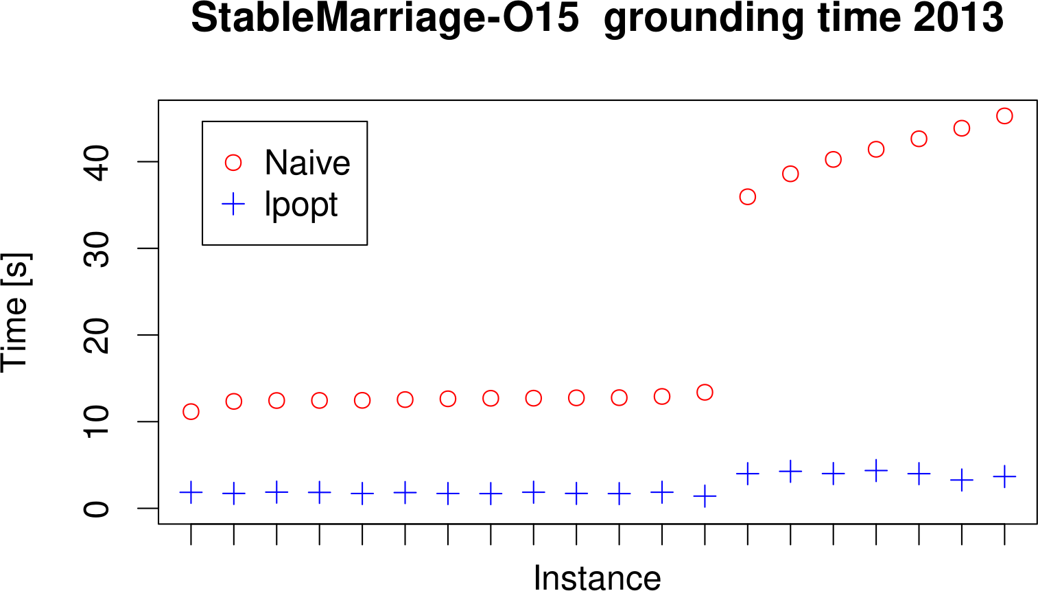
(a)

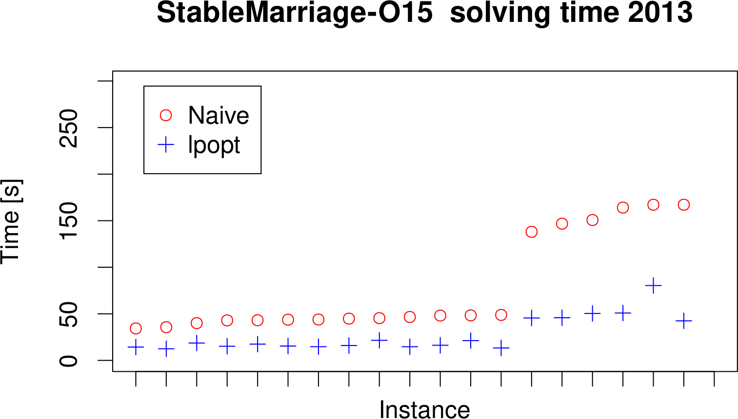
(b)

Figure 1: Benchmark results for the stable marriage 2013 instances. The horizontal axis represents the individual test instances, sorted by runtime without rule decomposition.

As can be seen in Figure 1, both grounding and solving time decrease dramatically. Notice that the grounding time is, in general, directly correlated with the size of the respective grounding. With lpopt preprocessing, the grounding size decreases dramatically by a factor of up to 65. The grounder is thirty times faster when using preprocessing, and the solver about three times. This is because of the following constraint in the encoding that can be decomposed very well:

:- match(M,W1), manAssignsScore(M,W,Smw), W1!=W,
     manAssignsScore(M,W1,Smw1), Smw>Smw1, match(M1,W),
     womanAssignsScore(W,M,Swm), womanAssignsScore(W,M1,Swm1),
     Swm>=Swm1.

The constraint rule above is quite intuitive to read: There cannot be a man $M$ and a woman $W$, such that they would both be better off if they were matched together, instead of being matched as they are (that is, to $W1$ and $M1$, respectively). It encodes, precisely and straightforwardly, the condition of a stable marriage. The 2014 encoding splits this rule up, making the encoding much harder to understand. However, with lpopt preprocessing, the grounding and solving performance matches that of the hand-tuned 2014 encoding. This again illustrates that the $\mathsf{lpopt}$ algorithm allows for efficient processing of rules written by non-experts that are not explicitly hand-tuned.

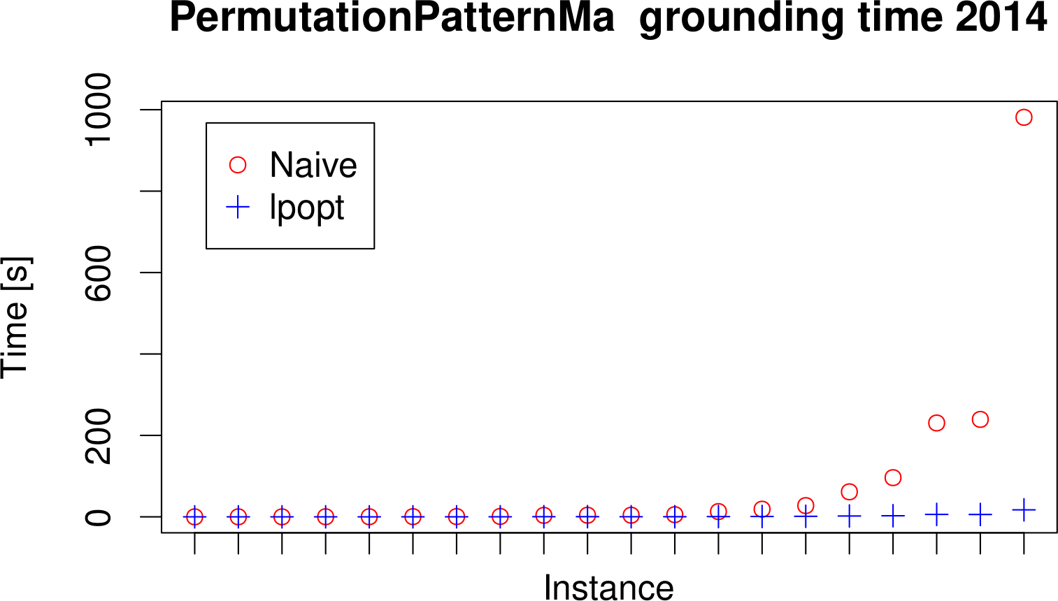
(a)

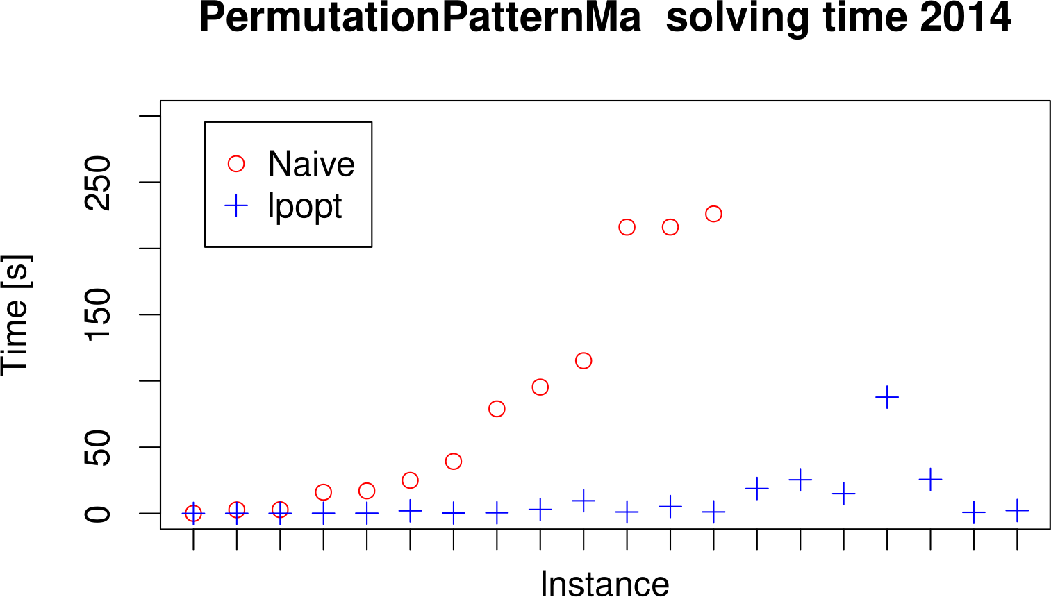
(b)

Figure 2: Benchmark results for permutation pattern matching 2014. The horizontal axis represents the individual test instances, sorted by runtime without rule decomposition.

A second example of lpopt’s capabilities is the permutation pattern matching problem illustrated in Figure 2. The grounding time of the largest instance is $980$ seconds without preprocessing and $17$ seconds with preprocessing. This instance was also impossible to solve within the timeout window of $300$ seconds without lpopt preprocessing, but finishing within $88$ seconds when lpopt was run first.

Other Use Cases.

lpopt has also been employed in other works that illustrate its performance benefits. In particular, several solvers for other formalisms rely on a rewriting to ASP in order to solve the original problem. Such rewritings can easily lead to the generation of large rules that current ASP solving systems are generally unable to handle. For example, in [16] ASP rewritings for several problems from the abstract argumentation domain, proposed in [9], are implemented. In Section 4.6 of the thesis, the performance benefits of lpopt are clearly demonstated for these rewritings. Interestingly, these rewritings also make heavy use of aggregates which goes to show that lpopt also handles these constructs well. Another example is [5], where multiple rewritings for $\Sigma_{\textrm{P}}^{\textrm{2}}$ and $\Sigma_{\textrm{P}}^{\textrm{3}}$-hard problems are proposed and then benchmarked, again showcasing that without lpopt these rewritings could not be solved by current ASP solvers in all but the most simple cases.

Limitations.

However, we also want to point out some limitations of the $\mathsf{lpopt}$ algorithm. When a domain predicate is used by the algorithm, the selection of atoms that generate this domain predicate is at the moment essentially random, since the greedy selection depends on the order of the atoms appearing in the rule. This approach, as discussed in Section 3, may thus not pick an optimal set of atoms. However, it depends on this selection how many ground rules this domain predicate rule will generate when passed to the grounder. Therefore, it may at the moment be the case that the increased grounding size caused by the domain predicate rules may destroy any benefit caused by splitting up the main rule. This is precisely what caused the increase in solving time for the five encodings out of 49 that lpopt was able to rewrite but where solving performance deteriorated. Clearly, this begs the question of what the best strategy is to select atoms to generate domain predicates. This is part of ongoing work.

6 Conclusions

In this paper, we present an algorithm, based on a prototype from [18], that allows the decomposition of large logic programming rules into smaller ones that current state-of-the-art answer set programming solvers are better equipped to handle. Our implementation handles the entire ASP-Core-2 language [10]. Benchmark results show that in practice, even for extensively hand-tuned ASP programs, our rule decomposition algorithm can improve solving performance significantly. Future work will include implementing this approach directly into state-of-the-art grounders like the gringo grounder used in our benchmarks, as well as further refining the algorithm w.r.t. selection of domain predicate atoms, as discussed at the end of Section 5.

Acknowledgments.

Funded by the Austrian Science Fund (FWF): Y698, P25607.

References

- [1] Alviano, M., Dodaro, C., Faber, W., Leone, N., Ricca, F.: WASP: A native ASP solver based on constraint learning. In: Proc. LPNMR. pp. 54–66 (2013), http://dx.doi.org/10.1007/978-3-642-40564-8_6
- [2] Alviano, M., Faber, W., Leone, N., Perri, S., Pfeifer, G., Terracina, G.: The disjunctive datalog system DLV. In: Datalog Reloaded. Revised Selected Papers. pp. 282–301 (2010), http://dx.doi.org/10.1007/978-3-642-24206-9_17
- [3] Arnborg, S., Corneil, D.G., Proskurowski, A.: Complexity of finding embeddings in a k-tree. SIAM J. Algeb. Discr. Meth. 8(2), 277–284 (1987), http://dx.doi.org/10.1137/0608024
- [4] Bichler, M.: Optimizing non-ground answer set programs via rule decomposition. BSc Thesis, TU Wien. http://dbai.tuwien.ac.at/proj/lpopt (2015)
- [5] Bichler, M., Morak, M., Woltran, S.: The power of non-ground rules in answer set programming. In: Proc. ICLP. To appear (2016), https://arxiv.org/abs/1608.01856
- [6] Bodlaender, H.L.: A linear-time algorithm for finding tree-decompositions of small treewidth. SIAM J. Comput. 25(6), 1305–1317 (1996), http://dx.doi.org/10.1137/S0097539793251219
- [7] Bodlaender, H.L., Koster, A.M.C.A.: Treewidth computations i. upper bounds. Inf. Comput. 208(3), 259–275 (2010), http://dx.doi.org/10.1016/j.ic.2009.03.008
- [8] Brewka, G., Eiter, T., Truszczynski, M.: Answer set programming at a glance. Commun. ACM 54(12), 92–103 (2011), http://doi.acm.org/10.1145/2043174.2043195
- [9] Brewka, G., Woltran, S.: GRAPPA: A semantical framework for graph-based argument processing. In: Proc. ECAI. pp. 153–158 (2014), http://dx.doi.org/10.3233/978-1-61499-419-0-153
- [10] Calimeri, F., Faber, W., Gebser, M., Ianni, G., Kaminski, R., Krennwallner, T., Leone, N., Ricca, F., Schaub, T.: ASP-Core-2 Input Language Format v2.03c (2015), https://www.mat.unical.it/aspcomp2013/ASPStandardization, accessed: 2016-06-27
- [11] Calimeri, F., Gebser, M., Maratea, M., Ricca, F.: Design and results of the fifth answer set programming competition. Artif. Intell. 231, 151–181 (2016), http://dx.doi.org/10.1016/j.artint.2015.09.008
- [12] Elkabani, I., Pontelli, E., Son, T.C.: Smodels - A system for computing answer sets of logic programs with aggregates. In: Proc. LPNMR. pp. 427–431 (2005), http://dx.doi.org/10.1007/11546207_40
- [13] Gebser, M., Kaminski, R., Kaufmann, B., Schaub, T.: Answer Set Solving in Practice. Synthesis Lectures on Artificial Intelligence and Machine Learning, Morgan & Claypool Publishers (2012), http://dx.doi.org/10.2200/S00457ED1V01Y201211AIM019
- [14] Gebser, M., Kaufmann, B., Schaub, T.: Conflict-driven answer set solving: From theory to practice. Artif. Intell. 187, 52–89 (2012), http://dx.doi.org/10.1016/j.artint.2012.04.001
- [15] Gelfond, M., Lifschitz, V.: The stable model semantics for logic programming. In: Proc. ICLP/SLP. pp. 1070–1080 (1988)
- [16] Heißenberger, G.: A System for Advanced Graphical Argumentation Formalisms. Master’s thesis, TU Wien (2016), www.dbai.tuwien.ac.at/proj/adf/grappavis/
- [17] Marek, V.W., Truszczyński, M.: Stable Models and an Alternative Logic Programming Paradigm. In: The Logic Programming Paradigm – A 25-Year Perspective, pp. 375–398. Springer (1999)
- [18] Morak, M., Woltran, S.: Preprocessing of complex non-ground rules in answer set programming. In: Proc. ICLP. pp. 247–258 (2012), http://dx.doi.org/10.4230/LIPIcs.ICLP.2012.247