On equivariant binary differential equations

Abstract

This paper introduces the study of occurrence of symmetries in binary differential equations (BDEs). These are implicit differential equations given by the zeros of a quadratic 1-form, $a(x,y)dy^{2}+b(x,y)dxdy+c(x,y)dx^{2}=0,$ for $a,b,c$ smooth real functions defined on an open set of $\mathbb{R}^{2}$. Generically, solutions of a BDE are given as leaves of a pair of foliations, and the action of a symmetry must depend not only whether it preserves or inverts the plane orientation, but also whether it preserves or interchanges the foliations. The first main result reveals this dependence, which is given algebraically by a formula relating three group homomorphisms defined on the symmetry group of the BDE. The second main result adapts algebraic methods from invariant theory for representations of compact Lie groups on the space of quadratic forms on $\mathbb{R}^{n},n\geq 2$. With that we obtain an algorithm to compute general expressions of quadratic forms. Now, symmetric quadratic 1-forms are in one-to-one correspondence with equivariant quadratic forms on the plane, so these are treated here as a particular case. The general forms of equivariant quadratic 1-forms under each compact subgroup of the orthogonal group ${\mathbf{O}(2)}$ are also given.

1 Introduction

A binary differential equation on the plane, or a BDE, is an implicit quadratic differential equation

$$a(x,y)dy^{2}+2b(x,y)dxdy+c(x,y)dx^{2}=0,$$ (1)

where the coefficients $a,b,c$ are real functions which we assume to be smooth on an open set $U\subseteq{\mathbb{R}}^{2}$. The function $\delta:U\rightarrow\mathbb{R},$ $\delta(x,y)=(b^{2}-ac)(x,y)$, is the discriminant function and its zero set

$$\Delta=\{(x,y)\in U:(b^{2}-ac)(x,y)=0\}$$

is the discriminant set of the BDE. The investigation of occurrence of symmetries is converted in purely algebraic terms, so there is no loss of generality in assuming that $U$ is the whole plane, which we do from now on for simplicity. At points where $\delta>0$, (1) defines a pair of transversal directions, and by the configuration associated with this equation we mean the distribution of all solution curves tangent to these directions. The geometry of a BDE configuration is a subject of great interest, with important applications in differential geometry, as the equations of lines of curvatures, characteristic curves and asymptotic curves of smooth surfaces, and in control theory (see [17] and references therein). Conditions for local stability of positive binary differential equations ($\delta>0$) and their classification are given in [10] and [11], with a description of the topological patterns that bifurcate in one-parameter families of these equations. Singular points of a class of positive binary equations associated with a smooth surface are also studied in[10] and [16], the coefficients of BDE being given in terms of the coefficients of the first and second fundamental forms of the surface. Determining models of configurations associated with BDEs has been also addressed in many works; for example, in [3, 4, 5, 6, 12, 18, 19] the classification of BDEs is performed up to topological, formal, analytic or smooth equivalences. We refer to [17] for a survey on these topics.

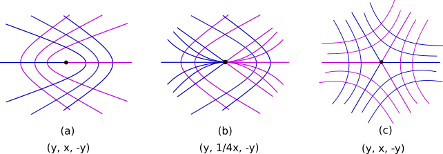
Figure 1: Configurations of symmetric BDEs. In (a) and (b) the symmetry group is $\mathbf{Z}_{2}\times\mathbf{Z}_{2}$ and in (c) the symmetry group is $\mathbf{D}_{6}$.

This work is motivated by the recognition of symmetries in most normal forms that appear in the works mentioned above. In the linear case for example, namely when the coefficients of (1) are linear functions, presence of at least one nontrivial symmetry (namely minus identity) is a necessary condition. As a consequence, our study shows which symmetry groups are attained or never attained in the nonlinear cases. The purpose of the present paper is to introduce the systematic study of symmetries in binary differential equations. [15] is a continuation of this study: we investigate symmetries of a BDE in connection with an associated pair of equivariant vector fields (see Remark 2.7); also, quadratic forms with homogeneous coefficients are studied through an analysis of the number of invariant lines that appear in the configuration space imposed by their group of symmetries; in addition, we analyse possible symmetry groups of BDEs with Morse type discriminant introduced in [3]. More recently we have driven attention to some questions relating symmetries in differential forms to pairs of foliations of special classes of surfaces; for example, for a given equivariant BDE, we ask whether this can be realized as an equation of lines of curvatures or of asymptotic lines of a surface immersed in ${\mathbb{R}}^{n}$ for some $n$.

To remark on evidences of occurrence of symmetries in configurations associated with BDEs, let us consider the configurations that appear in [2], which are generic topological structures of principal direction fields at umbilic points of surfaces on Euclidean spaces. The normal forms are given as triples $(a,b,c)$ for $c=\pm a$ in (1) and their configurations are reproduced in Fig. 1, the so-called (a) lemon, (b) monstar and (c) star. The solution curves determine two foliations of the plane distinguished by colour, and the black point is the discriminant set. The pictures clearly suggest an invariance of the three configurations under reflection with respect to the $x$-axis. There is another invariance with respect to the $y$-axis, which is given by this operation followed by a change of colour. As a consequence, the composition of these two elements (minus identity) must be a symmetry which interchanges colour. In fact, we should recognize a priori minus identity in the set of symmetries of all these cases by their linearity, as mentioned above. The third picture has also six rotational symmetries, three of which are colour-preserving and the other three are colour-interchanging. In fact, the full symmetry group of pictures (a) and (b) is ${\bf Z}_{2}\times{\bf Z}_{2}$, generated by the reflections across the axes, and the full symmetry group of picture (c) is the dihedral group $\mathbf{D}_{6}$, generated by a reflection and a rotation of order six. As these examples illustrate, the group action must be defined taking colour changes into consideration at the region on the plane where (1) defines a bivalued direction field. As we shall see, the action of a symmetry group $\Gamma$ of a binary differential equation must be defined on the tangent bundle through its representation on the plane combined with a group homomorphism $\eta:\Gamma\to{\bf Z}_{2}=\{\pm 1\}$ (Definition 2.2). This action is translated into an action of $\Gamma$ on the space of symmetric matrices under conjugacy. This is then used to obtain the general forms of equivariant BDEs under all compact subgroups of ${\bf O}(2)$ through invariant theory.

The paper is organized as follows: in Section 2 we introduce the notion of symmetries in a BDE, namely when the equation is invariant under the linear action of a subgroup $\Gamma\leq{\bf O}(2)$. We formalize the concept using group representation theory on the tangent bundle on which the associated quadratic 1-form is defined. One of our two main results is Theorem 2.4, which establishes a formula that reveals the effect of a symmetry in the configuration geometry in simple algebraic terms. In Section 3 we generalize the results in [1] for $\Gamma$-equivariant mappings with distinct actions on the source and target. The results allow the computation of general forms of equivariant mappings using an algebraic algorithm (Algorithm 3.3). In Section 4 we implement these results to calculate the general forms of equivariant BDEs under any compact subgroup of ${\bf O}(2)$, which is our second main result, summarized in Table 1; in this section we also present a number of examples.

2 Symmetry groups of binary differential equations

In this section we formalize the concept of a symmetric binary differential equation under the linear action of a compact Lie subgroup $\Gamma$ of $\mathbf{O}(2)$ .

Let ${\cal F}({\mathbb{R}}^{2})$ denote the set of real $C^{\infty}$ quadratic differential forms $\omega$ on $M={\mathbb{R}}^{2}$, $\omega:TM\to{\mathbb{R}}$ defined on the tangent bundle $TM=\sqcup_{u\in M}T_{u}M$ given by

$$\omega=a(x,y)dy^{2}+2b(x,y)dxdy+c(x,y)dx^{2},$$ (2)

with $a,b,c$ $C^{\infty}$ functions on ${\mathbb{R}}^{2}$. Let $\Gamma$ be a compact Lie group acting linearly on $\mathbb{R}^{2}$. This induces an action of $\Gamma$ on the tangent bundle,

$$\begin{array}[]{ccc}\Gamma\times\sqcup_{u\in M}T_{u}M&\to&\sqcup_{u\in M}T_{u}M\\ (\gamma,u,v)&\mapsto&\gamma\cdot(u,v)\ =\ \bigl{(}\gamma u,(d\gamma\bigr{)}_{u}(v)).\end{array}$$

Since the action is linear, $\gamma\cdot(u,v)=(\gamma u,\gamma v)$.

Let $\eta:~{}\Gamma~{}\rightarrow~{}\mathbf{Z}_{2}~{}=~{}\{\pm 1\}$ be a one-dimensional representation of $\Gamma$, acting on the target of $\omega$. We then give the following:

Definition 2.1.

An element $\omega\in{\cal F}({\mathbb{R}}^{2})$ is $\Gamma_{\eta}$-equivariant if, for all $\gamma\in\Gamma$,

$$\omega(\gamma\cdot(x,y,dx,dy))\ =\ \eta(\gamma)\omega(x,y,dx,dy).$$ (3)

The BDE (1) is the equation of zeros of (2), so we define

Definition 2.2.

For $\Gamma$ a compact Lie group acting linearly on ${\mathbb{R}}^{2}$ and $\eta:~{}\Gamma~{}\rightarrow~{}\mathbf{Z}_{2}$ a group homomorphism, the binary differential equation $(\ref{BDE})$ is $\Gamma$-invariant, or $\Gamma$ is the symmetry group of $(\ref{BDE})$, if $\omega$ in $(\ref{eq:1-form})$ is $\Gamma_{\eta}$-equivariant.

We notice that the group of symmetries of a BDE generally admits, by its nature, an order-2 normal subgroup, which is equivalent to saying that the group homomorphism $\eta$ in Definition 2.2 is nontrivial. Hence, in the present context, symmetries are established through the group together with this homomorphism, and hence this action is denoted below by $\Gamma_{\eta}$.

Remark 2.3.

Let $\Sigma(\Delta)\leq{\bf O}(2)$ denote the group of symmetries of $\Delta$, namely, the subgroup of elements of ${\bf O}(2)$ that leave $\Delta$ setwise invariant. Then

$$\Gamma_{\eta}\leq\Sigma(\Delta).$$ (4)

In other words, symmetries of a BDE are at most the symmetries of the discriminant set. This can be of practical use when detecting the symmetry group of the equation if we know the shape of $\Delta$.

Solutions of (1) are nonoriented curves, associated with direction fields. At the region on the plane where the discriminant $\delta$ is positive, these form a pair of transverse foliations ${\mathscr{F}}_{1}$ and ${\mathscr{F}}_{2}$. The set of symmetries of each foliation, that is, the set of elements that leave them setwise invariant is a subgroup of $\Gamma$. The structure of this subgroup is discussed below. This pair is, in turn, associated with two oriented foliations given as integral curves of the vector fields

$$X_{i}(x,y)\ =\ (a(x,y),b(x,y)+(-1)^{i}\sqrt{\delta(x,y)}),\ \ i=1,2.$$ (5)

Consider for example the equation

$$\omega(x,y)=ydy^{2}+2xdxdy-ydx^{2}=0,$$

for which the associated vector fields are

$$X_{i}(x,y)\ =\ (y,x+(-1)^{i}\sqrt{x^{2}+y^{2}}),\ \ i=1,2.$$

The configuration of this equation is given in Fig. 1(a). Both $X_{1}$ and $X_{2}$ are reversible-equivariant vector fields under the action of the group $\mathbf{Z}_{2}$ generated by the reflection $\kappa_{x}$ with respect to the $x$-axis,

$$X_{i}(\kappa_{x}(x,y))\ =\ -\kappa_{x}X_{i}(x,y),\\ i=1,2.$$

As the picture suggests, this reflection is in fact a symmetry of the BDE. Now, the combination of the two foliations adds symmetries to the whole picture, leading to a configuration which is also symmetric with respect to the reflection on the $y$-axis. By the nature of this additional symmetry, this element should invert foliations. In fact, we prove that $\mathbf{Z}_{2}\times\mathbf{Z}_{2}$ is the symmetry group of the BDE. However, it is more subtle to realize how each element should act on the form $\omega$, in the sense that it is not obvious whether $\eta(\gamma)=1$ or $-1$ for each $\gamma$ in the group. As we shall see in Theorem 2.4, this depends not only whether $\gamma$ preserves or interchanges foliations, but also whether it preserves or inverts orientation on the plane.

Before we state the result, we introduce another homomorphism: Consider the open region in ${\mathbb{R}}^{2}$

$$\Omega=\{(x,y)\in{\mathbb{R}}^{2}\ :\ \delta(x,y)>0\},$$

and consider the restriction of the action of $\Gamma_{\eta}$ on $\Omega$. This is well-defined since the discriminant set $\Delta$ is $\Gamma$-invariant and splits the plane into two invariant regions, where $\delta$ is positive or negative. For BDEs (1) for which $\Omega$ is non-empty, we introduce the homomorphism $\lambda:\Gamma\to\mathbf{Z}_{2}=\{\pm 1\}$,

$$\lambda(\gamma)=\left\{\begin{array}[]{cl}1,&\gamma({\mathscr{F}}_{i})={\mathscr{F}}_{i}\\ -1,&\gamma({\mathscr{F}}_{i})={\mathscr{F}}_{j},\ j\neq i,\end{array}\right.$$ (6)

$i,j\in\{1,2\}$. It follows directly from this definition that the subgroup of symmetries of each foliation ${\mathscr{F}}_{i}$, $i=1,2$, is $\Sigma({\mathscr{F}}_{i})=\ker\lambda$.

Theorem 2.4.

Let  $\eta,\ \lambda:\Gamma\to\mathbf{Z}_{2}$ be the two group homomorphisms of Definition 2.2 and of $(\ref{eq:lambda})$. Then, for all $\gamma\in\Gamma$,

$$\lambda(\gamma)=\det(\gamma)\ \eta(\gamma).$$

Proof.

At $(x,y)\in\Omega$ consider the pair of tangent vectors given in (5),

$$X_{i}(x,y)=(a(x,y),-b(x,y)+(-1)^{i}\sqrt{\delta(x,y)}),\ i=1,2.$$

From the definition of the action $\Gamma$ on $TM$, the pair of tangent vectors to the two solution curves at $\gamma(x,y)$ is given by $\gamma X_{i}(x,y)$, $i=1,2$. On the other hand, from the equivariance of $\omega$ under $\Gamma_{\eta}$, the vectors

$$X_{i}(\gamma(x,y))=(\eta a(x,y),-\eta b(x,y)+(-1)^{i}\sqrt{\delta(x,y)}),\ i=1,2,$$

are also tangent vectors to the two solution curves at $\gamma(x,y)$. By symmetry it follows that these two pairs must be parallel, i.e., there exists a nonzero $\alpha$ such that, for $i\neq j\in\{1,2\},$

$$\gamma X_{i}(x,y)=\left\{\begin{array}[]{ll}\alpha X_{i}(\gamma(x,y)),&\hbox{if}\ \lambda(\gamma))=1\\ \alpha X_{j}(\gamma(x,y)),&\hbox{if}\ \lambda(\gamma))=-1.\end{array}\right.$$ (7)

Also, by the orthogonality of the action, we have $\alpha=\pm 1$. Now, consider the two matrices $M_{1}$ and $M_{2}$ whose columns are the vectors $\gamma X_{1},\gamma X_{2}$ and $X_{1}\gamma,X_{2}\gamma$ both calculated at $(x,y)$, respectively, that is,

$$M_{1}=\left(\begin{array}[]{cc}\gamma X_{1}&\gamma X_{2}\\ \end{array}\right),\ M_{2}=\left(\begin{array}[]{cc}\eta(\gamma)a&\eta(\gamma)a\\ -\eta(\gamma)b-\sqrt{\delta}&-\eta(\gamma)b+\sqrt{\delta}\\ \end{array}\right)$$

From (7) it follows that

$$\det(M_{1})=\alpha^{2}\lambda(\gamma)\det(M_{2})=\lambda(\gamma)\det(M_{2}).$$

Finally, $\det(M_{1})=\det(\gamma)\ 2a\sqrt{\delta}$, and $\det(M_{2})=\eta(\gamma)2a\sqrt{\delta}$. Hence,

$$\det(\gamma)=\eta(\gamma)\lambda(\gamma),$$

which implies the result since these are all group homomorphisms $\Gamma\to\mathbf{Z}_{2}=\{\pm 1\}$. ∎

Remark 2.5.

In practice, Theorem 2.4 adds information to the inclusion $(\ref{eq: inclusion})$ when detecting the symmetry group $\Gamma_{\eta}$ of a BDE. In fact, it provides the construction of the homomorphism $\eta$ by the geometrical investigation of whether each element $\gamma\in\Gamma_{\eta}$ preserves the foliations ($\lambda(\gamma)=1$) or interchanges the foliations ($\lambda(\gamma)=-1$). To illustrate, consider the pictures in Fig. 1. In $(a)$ and $(b)$, foliations are interchanged by $\kappa_{y}$, whereas they are preserved by $\kappa_{x}$, and now we use $\det(\kappa_{x})=\det(\kappa_{y})=-1$ to conclude by Theorem 2.4 that $\eta(\kappa_{x})=-\eta(\kappa_{y})=-1$. These are the generators of the symmetry group $\mathbf{Z}_{2}\times\mathbf{Z}_{2}$, and so the homomorphism $\eta$ is well-established for these examples. In $(c)$ foliations are interchanged by $\kappa_{y}$ and rotation of $\pi/3$; since these are orientation reserving and orientation preserving respectively, it follows that $\eta$ assumes $1$ and $-1$, respectively. These are the generators of the symmetry group ${\bf D}_{6}$, and so the homomorphism $\eta$ is well-established.

The following property is direct from Theorem 2.4:

Corollary 2.6.

$\ker\lambda\cap\ker\eta$ is a cyclic group of $\Gamma$.

A quadratic differential form (2) is associated to the matrix-valued mapping $B:\mathbb{R}^{2}\rightarrow Sym_{2},$

$$B(x,y)=\left(\begin{array}[]{cc}c(x,y)&b(x,y)\\ b(x,y)&a(x,y)\\ \end{array}\right),$$ (8)

where $Sym_{2}$ denotes the set of symmetric matrices of order 2. Then (2) can be written as

$$\omega\ =\ \left(\begin{array}[]{c}dx\\ dy\\ \end{array}\right)^{t}\ B(x,y)\ \left(\begin{array}[]{c}dx\\ dy\\ \end{array}\right),$$

where superscript $t$ denotes transposition. From (3), it follows that symmetries of (1) are given by the following equivariance condition of $B$, with the action on the target given by the homomorphism $\eta$ and conjugacy:

$$B\bigl{(}\gamma(x,y)\bigr{)}=\eta(\gamma)\gamma B(x,y)\gamma^{t},\ \forall\ \gamma\in\Gamma.$$ (9)

Remark 2.7.

Although Definition 2.1 is given here for quadratic 1-forms, the equivariance condition $(\ref{eq:equivariant form})$ can be given for general 1-forms. For the linear case, it follows that

$$\alpha(x,y,dx,dy)=A(x,y)dy+B(x,y)dx$$

is $\Gamma_{\eta}$-equivariant if, and only if, the associated planar mapping $F=(A,B)$ is $\Gamma_{\eta}$-equivariant in the sense of Definition 3.1 below. For an investigation of pairs of symmetric linear 1-forms and their connection with symmetries of an associated BDE we refer to [15].

From now on we shall use the matricial notation (9) to investigate symmetries in BDEs. For a given $\Gamma_{\eta}$, the aim is to find the general form of symmetric matrices (8) satisfying (9). This is an algebraic problem which is treated in Section 4.

3 Invariant theory for the group $\Gamma_{\eta}$

The aim of this section is to obtain generalizations of some results of [1] to be applied to a systematic study of symmetries in BDEs. The idea is to use group representation theory in the study of symmetries in the space of quadratic forms. In Subsection 3.1 we register the generalization of results of [1] to $\Gamma_{\eta}$-equivariant mappings $V\to W$ (possibly distinct source and target), whose proofs adapt straightforwardly from [1]. In Subsection 3.2 we restrict the results of the preceding subsection to equivariant mappings ${\mathbb{R}}^{n}\to Sym_{n}$, where $Sym_{n}$ denotes the space of symmetric matrices of order $n$. These are then used in Section 4 in the study of symmetries in binary differential equations.

3.1 $\Gamma_{\eta}$-equivariant mappings

We start with a brief summary about algebraic invariant theory of compact Lie groups. Throughout we consider a compact Lie group $\Gamma$ acting linearly on a real vector space $V$ of finite dimension $n$. There exists a $\Gamma$-invariant inner product on $V$ under which the representation $(\rho,V)$ associated with the given action of $\Gamma$ is orthogonal, i.e. for $\gamma\in\Gamma$, $\rho(\gamma)\in\mathbf{O}(n)$, the group of orthogonal matrices of order $n$ ([9, XII, Proposition 1.3]). Hence, Lie groups in this paper are the closed subgroups of $\mathbf{O}(n)$. A real function $f:V\rightarrow\mathbb{R}$ is $\Gamma$-invariant if

$$f(\rho(\gamma)x)=f(x),\ \ \forall\ \gamma\in\Gamma,\ \forall\ x\in V.$$

The set $\mathcal{P}(\Gamma)$ of $\Gamma$-invariant polynomials is a ring over $\mathbb{R}$. A finite set $\{u_{1},...u_{s}\}$ of $\Gamma$-invariants generating this ring is called a Hilbert basis for $\mathcal{P}(\Gamma).$ The existence of a Hilbert basis was proved by Weyl in $1946$, and Schwarz proved in $1975$ that the same set generates the ring of $C^{\infty}$ $\Gamma$-invariant germs (see [9]).

For $(\rho,V)$ and $(\nu,W)$ representations of $\Gamma,$ a mapping $g:V\rightarrow W$ is $\Gamma$-equivariant if

$$g(\rho(\gamma))=\nu(\gamma)g(x),\ \ \forall\ \gamma\in\Gamma,\ \forall x\in V.$$

The set $\overrightarrow{\mathcal{P}}(\Gamma)$ of $\Gamma$-equivariant mappings $V\to W$ with polynomial entries is a module over $\mathcal{P}(\Gamma)$. Poénaru in 1976 proved that $\overrightarrow{\mathcal{P}}(\Gamma)$ is finitely generated over the ring $\mathcal{P}(\Gamma)$ and that the same set generates the module of equivariant $C^{\infty}$ germs over the ring of invariant germs.

We shall also consider a one-dimensional representation of $\Gamma$,

$$\eta:\Gamma\rightarrow\mathbf{Z}_{2}=\{\pm 1\}.$$ (10)

This is a group homomorphism with $\Gamma_{+}=\ker\eta$ a normal subgroup of $\Gamma$ of index $2$ if $\eta$ is nontrivial. From that, we also have the so-called $\eta$-dual representation of $(\nu,W)$, denoted by $\nu_{\eta}$, defined by the product

$$\gamma\mapsto\nu_{\eta}(\gamma)=\eta(\gamma)\nu(\gamma).$$

Definition 3.1.

For $\eta$ as in $(\ref{homom eta})$ and $(\rho,V)$ and $(\nu,W)$ representations of $\Gamma$, a function $f:V\rightarrow\mathbb{R}$ is $\Gamma_{\eta}$-invariant if

$$f(\rho(\gamma)x)=\eta(\gamma)f(x),\ \ \forall\ \gamma\in\Gamma,\ \forall\ x\in V.$$

A mapping $g:V\rightarrow W$ is $\Gamma_{\eta}$-equivariant if

$$g(\rho(\gamma)x)=\eta(\gamma)\nu(\gamma)g(x),\ \ \forall\ \gamma\in\Gamma,\ \forall\ x\in V.$$

We shall denote $\overrightarrow{\mathcal{P}}^{\eta}(\Gamma)$ and $\mathcal{P}^{\eta}(\Gamma)$ the sets of $\Gamma_{\eta}$-equivariant polynomial mappings and $\Gamma_{\eta}$-invariant polynomial functions, respectively. A $\Gamma_{\eta}$-equivariant is an equivariant $(\rho,V)\to(\nu_{\eta},W)$, and a $\Gamma_{\eta}$-invariant is an equivariant $(\rho,V)\to(\eta,\mathbb{R})$, so the finitude of generators for each as $\mathcal{P}(\Gamma)$-modules follows by Poénaru’s theorem. It also follows from this theorem that it is no loss of generality to restrict to modules of polynomials when finding generators of $C^{\infty}$ mappings. In Section 4 we shall see how configurations change when the symmetry group of binary differential equations changes to its dual representation.

A connection is established in [1] between the invariant theory for $\Gamma$ and $\Gamma_{+}$. This is done through an algebraic algorithm to compute generators of $\overrightarrow{\mathcal{P}}^{\eta}(\Gamma)$ from the knowledge of generators of $\overrightarrow{\mathcal{P}}(\Gamma_{+})$, when source and target spaces are the same. In Proposition 3.2 and Algorithm 3.3 we generalize this, with a similar algorithm to compute generators of $\Gamma_{\eta}$-equivariants with possibly distinct source and target.

We follow the notation used in [1] to introduce the Reynolds operators $R:~{}\mathcal{P}(\Gamma_{+})~{}\rightarrow~{}\mathcal{P}(\Gamma_{+})$ and $\overrightarrow{R}:\overrightarrow{\mathcal{P}}(\Gamma_{+})\rightarrow\overrightarrow{\mathcal{P}}(\Gamma_{+})$,

$$R(f)(x)=1/2(f(x)+f(\rho(\delta)x))\ \ \mbox{e}\ \ \overrightarrow{R}(g)(x)=1/2(g(x)+\nu(\delta)^{-1}g(\rho(\delta)x)),$$

and, the $\eta$-Reynolds operators on $\mathcal{P}(\Gamma_{+})$ and on $\overrightarrow{\mathcal{P}}(\Gamma_{+})$, $S:\mathcal{P}(\Gamma_{+})\rightarrow\mathcal{P}(\Gamma_{+})$ and $\overrightarrow{S}:\overrightarrow{\mathcal{P}}(\Gamma_{+})\rightarrow\overrightarrow{\mathcal{P}}(\Gamma_{+})$,

$${S}(f)(x)=1/2(f(x)-f(\rho(\delta)x))\ \ \mbox{e}\ \ \overrightarrow{S}(g)(x)=1/2(g(x)-\nu(\delta)^{-1}g(\rho(\delta)x)),$$

for an arbitrary fixed $\delta\in\Gamma\setminus\Gamma_{+}$.

Let us denote by $I_{\mathcal{P}(\Gamma_{+})}$ and $I_{\small\overrightarrow{\mathcal{P}}(\Gamma_{+})}$ the identity maps on $\mathcal{P}(\Gamma_{+})$ and on $\overrightarrow{\mathcal{P}}(\Gamma_{+})$, respectively.

Proposition 3.2.

The operators above satisfy the following:

(a)

They are homomorphisms of $\mathcal{P}(\Gamma)$-modules and

$$R+S=I_{\mathcal{P}(\Gamma_{+})}\ \ \ \mbox{and}\ \ \ \overrightarrow{R}+\overrightarrow{S}=I_{\small\overrightarrow{\mathcal{P}}(\Gamma_{+})}.$$

(b)

They are idempotent projections and the following direct sum decompositions of $\mathcal{P}(\Gamma)$-modules hold:

$$\mathcal{P}(\Gamma_{+})=\mathcal{P}(\Gamma)\oplus\mathcal{P}^{\eta}(\Gamma)\ \ \ \mbox{and}\ \ \ \overrightarrow{\mathcal{P}}(\Gamma_{+})=\overrightarrow{\mathcal{P}}(\Gamma)\oplus\overrightarrow{\mathcal{P}}^{\eta}(\Gamma).$$ (11)

Proof.

Analogous to Propositions 2.3 and 2.4 in [1]. ∎

The algorithm is based on the decompositions (11) and on the projection operators $S$ and $\overrightarrow{S}$ applied to a given Hilbert basis of $\mathcal{P}(\Gamma_{+})$ and a set of generators of $\overrightarrow{\mathcal{P}}(\Gamma_{+})$. The procedure is:

Algorithm 3.3.

Let $\Gamma$ be a closed subgroup of $\mathbf{O}(n)$ and $\eta:\Gamma\rightarrow\mathbf{Z}_{2}$ a homomorphism with $\ker\eta=\Gamma_{+}$, $\{u_{1},...,u_{s}\}$ a Hilbert basis of $\mathcal{P}(\Gamma_{+})$ and $\{H_{0},...,H_{r}\}$ a generator set of $\overrightarrow{\mathcal{P}}(\Gamma_{+})$ as a $\mathcal{P}(\Gamma_{+})$-module;

1

Fix $\delta\in\Gamma\setminus\Gamma_{+}$ arbitrary;

2

For $i\in\{1,...,s\}$, do $\tilde{u}_{i}=S(u_{i}),\tilde{u_{0}}:=1;$

3

For $i\in\{1,...,s\}$ and $j\in\{0,...,r\}$, do $H_{ij}=\tilde{u}_{i}H_{j};$

4

For $i\in\{1,...,s\}$ and $j\in\{0,...,r\}$, do $\tilde{H}_{ij}=\overrightarrow{S}(H_{ij})$.

Result: $\{\tilde{H}_{ij}:\ 0\leq i\leq s,\>0\leq j\leq r\}$ is a generator set of $\overrightarrow{\mathcal{P}}^{\eta}(\Gamma)$ as a $\mathcal{P}(\Gamma)$-module.

As proved in [1], step 2 above provides a generator set of the $\mathcal{P}(\Gamma)$-module $\mathcal{P}^{\eta}(\Gamma)$ (these are the anti-invariants in that paper). What we also remark at this point is that replacing $\overrightarrow{S}$ by the projection operator $\overrightarrow{R}$ in step 4 we obtain, as expected, a direct way to compute a set of generators for the equivariants under the whole group $\Gamma$ from the knowledge of equivariants under the subgroup $\Gamma_{+}$. This is formalized below:

Proposition 3.4.

Let $\Gamma$ be a compact Lie group acting on $V$ and on $W$ and $\{H_{ij}=\tilde{u}_{i}H_{j},0\leq i\leq s,0\leq j\leq r\}$ a generator set of $\overrightarrow{\mathcal{P}}(\Gamma_{+})$ as a $\mathcal{P}(\Gamma)$-module given by step $3$ in Algorithm 3.3). Then

$$\{\overrightarrow{R}(H_{i,j}),0\leq i\leq s,0\leq j\leq r\}$$

generates $\overrightarrow{\mathcal{P}}(\Gamma)$ as a $\mathcal{P}(\Gamma)$-module.

Proof.

Let $g\in\overrightarrow{\mathcal{P}}(\Gamma)\subset\overrightarrow{\mathcal{P}}(\Gamma_{+})$. Then $g=\sum_{i,j}^{s,r}p_{ij}H_{ij},\ \ \ p_{ij}\in\mathcal{P}(\Gamma),$ $0\leq i\leq s$ e $0\leq j\leq r$. Since $\overrightarrow{R}$ is a $\mathcal{P}(\Gamma)$-homomorphism and $\overrightarrow{R}(g)=g$, then

$$g=\overrightarrow{R}(g)=\overrightarrow{R}\left(\sum_{i,j}^{s,r}p_{ij}H_{ij}\right)=\sum_{i,j}^{s,r}p_{ij}\overrightarrow{R}(H_{ij}).$$

∎

3.2 $\Gamma_{\eta}$-equivariant quadratic forms

Let $\Gamma$ be a closed subgroup of $\mathbf{O}(n)$ acting linearly on $\mathbb{R}^{n}$. In this subsection we just rewrite the Reynolds operators of Subsection 3.1 applied to the module of $\Gamma_{\eta}$-equivariant quadratic forms of ordem $n$. In the present context, the representation on the target is defined from the representation on the source by conjugacy.

We consider the action of $\Gamma$ on $Sym_{n}$, the space of symmetric matrices of order $n$, given by conjugacy,

$$(\gamma,B)\mapsto\gamma B\gamma^{t},\ \gamma\in\Gamma,\ B\in Sym_{n}.$$

Definition 3.5.

A quadratic form of order $n$ is a matrix-valued mapping $B:\mathbb{R}^{n}\rightarrow Sym_{n}$.

Following the notation of Subsection 3.1, $\overrightarrow{\mathcal{P}}(\Gamma)$ is the module of the $\Gamma$-equivariants

$$B(\gamma x)=\gamma B(x)\gamma^{t},\ \ \forall\gamma\in\Gamma,\ x\in\mathbb{R}^{n},$$

and for $\eta:\Gamma\rightarrow\mathbf{Z}_{2}=\{\pm 1\}$ a nontrivial group homomorphism, $\overrightarrow{\mathcal{P}}^{\eta}(\Gamma)$ is the module of the $\Gamma_{\eta}$-equivariants

$$B(\gamma x)=\eta(\gamma)\gamma B(x)\gamma^{t},\ \ \forall\gamma\in\Gamma,\ x\in\mathbb{R}^{n}.$$

The Reynolds operators $\overrightarrow{R},\overrightarrow{S}:\overrightarrow{\mathcal{P}}(\Gamma_{+})\rightarrow\overrightarrow{\mathcal{P}}(\Gamma_{+}),$ are now

$$\overrightarrow{R}(g)(x)=1/2(g(x)+\delta^{-1}g(\delta x)\delta),\ \ \overrightarrow{S}(g)(x)=1/2(g(x)-\delta^{-1}g(\delta x)\delta),$$

for an arbitrary fixed $\delta\in\Gamma\setminus\Gamma_{+}$.

4 General forms of symmetric BDEs

The aim of this section is to present the algebraic forms of BDEs symmetric under the compact subgroups of ${\bf O}(2)$ with its standard action on the plane. These are derived from generator sets of the modules of equivariant quadratic forms on the plane

$$B(x,y)=\left(\begin{array}[]{cc}c(x,y)&b(x,y)\\ b(x,y)&a(x,y)\\ \end{array}\right).$$ (12)

These modules are $\overrightarrow{\mathcal{P}}(\Gamma)$ or $\overrightarrow{\mathcal{P}}^{\eta}(\Gamma)$ of Subsection 3.2 for $n=2$. If the group homomorphism $\eta:\Gamma\to\mathbf{Z}_{2}$ is nontrivial we apply Algorithm 3.3. For clarification of exposition, for each $\Gamma$ and for each possible $\eta$ we shall denote $\Gamma_{\eta}$ by $\Gamma[\ker\eta]$ when $\eta$ is nontrivial, and by $\Gamma$ otherwise. We also denote $\mathcal{P}^{\eta}(\Gamma)$ by $\mathcal{P}[\Gamma,\ker\eta]$ and $\overrightarrow{\mathcal{P}}^{\eta}(\Gamma)$ by $\overrightarrow{\mathcal{P}}[\Gamma,\ker\eta]$.

For the computations below we shall use the action of (subgroups of) $\mathbf{O}(2)$ on $\mathbb{R}^{2}\simeq\mathbb{C}$ with the usual semi-direct product of $\mathbf{SO}(2)$ and $\mathbf{Z}_{2}(\kappa)$, using complex coordinates,

$$\theta\cdot z=e^{i\theta}z,\ \ \hbox{and}\ \ \kappa z=\bar{z},\ \ \theta\in[0,2\pi],\ z\in\mathbb{C}.$$

In Subsections 4.1 and 4.2 we derive the general forms of symmetric BDEs under the cyclic group $\mathbf{Z}_{n}$, $n\geq 3$, and in Subsection 4.3 the general forms under ${\mathbf{Z}}_{2}$, for all possible homomorphisms $\eta$. For the other compact subgroups of ${\bf O}(2)$ the computation is similar and shall be omitted. In Subsection 4.4 all general forms are given in Table 1.

4.1 $\mathbf{Z}_{n}$-equivariant quadratic forms

Here we consider the cyclic group $\mathbf{Z}_{n}$, $n\geq 3$, with $\eta$ trivial. We compute generators of $\overrightarrow{\mathcal{P}}(\mathbf{Z}_{n})$ by computing generators of $\mathcal{M}(\mathbf{Z}_{n})$, the module of $\mathbf{Z}_{n}$-equivariant matrix-valued mappings $\mathbb{R}^{2}\to M_{2}(\mathbb{R}^{2})$, and projecting onto the space of mappings $\mathbb{R}^{2}\to Sym_{2}$ . In complex coordinates we write any element of $\mathcal{M}(\mathbf{Z}_{n})$ as

$$z\mapsto\alpha(z)w+\beta(z)\bar{w},\ \forall w\in{\mathbb{R}^{2}},$$ (13)

for functions $\alpha=\alpha_{1}+i\alpha_{2}$ and $\beta=\beta_{1}+i\beta_{2}$, with $\alpha_{j},\beta_{j},j=1,2$, real functions. Associating it with the real matrix

$$M=\left(\begin{array}[]{cc}\alpha_{1}+\beta_{1}&\beta_{2}-\alpha_{2}\\ \alpha_{2}+\alpha_{2}&\alpha_{1}-\beta_{1}\\ \end{array}\right),$$

the desired quadratic forms are obtained by the projection

$$M\mapsto B=1/2(M+M^{t}),$$ (14)

after imposing the $\mathbf{Z}_{n}$-symmetry condition. Write (13) as

$$M(z)w=\sum\alpha_{jk}z^{j}\bar{z}^{k}w+\sum\beta_{jk}z^{j}\bar{z}^{k}\bar{w},\ \ \ \ \alpha_{jk},\beta_{jk}\in\mathbb{C}.$$

The equivariance with respect to $\theta\in\mathbf{Z}_{n}$ gives

$$M(z)w=\sum\alpha_{jk}e^{i\theta(j-k)}z^{j}\bar{z}^{k}w+\sum\beta_{jk}e^{i\theta(j-k-2)}z^{j}\bar{z}^{k}\bar{w}.$$ (15)

So $\alpha_{jk}=\alpha_{jk}e^{i\theta(j-k)}$ and $\beta_{jk}=\beta_{jk}e^{i\theta(j-k-2)}$ for $\theta={2k\pi}/{n},\ k=1,\ldots,n$, and so

$$\alpha_{jk}=0\ \mbox{ou}\ j\equiv k\mbox{(mod n)}\ \ \ \mbox{and}\ \ \ \beta_{jk}=0\ \mbox{ou}\ \ j\equiv k+2\mbox{(mod n)}.$$ (16)

A Hilbert basis for $\mathcal{P}(\mathbf{Z}_{n})$ is given in [7],

$$\{u_{1}=z\bar{z},u_{2}=z^{n}+\bar{z}^{n},u_{3}=i(z^{n}-\bar{z}^{n})\}.$$

Factor out $z\bar{z}$ in (15) and use (16) to get

$$M(z)w = \sum_{j\geq k}\alpha_{jk}(z\bar{z})^{k}z^{j-k}w+\sum_{j<k}\alpha_{jk}(z\bar{z})^{j}\bar{z}^{k-j}w+\sum_{j\geq k}\beta_{jk}(z\bar{z})^{k}z^{j-k}\bar{w}+$$

$$+ \sum_{j<k}\beta_{jk}(z\bar{z})^{j}\bar{z}^{j-k}\bar{w}\ =\ \sum c^{1}_{kl_{1}}(z\bar{z})^{k}z^{l_{1}n}w+\sum c^{2}_{jl_{2}}(z\bar{z})^{j}\bar{z}^{l_{2}n}w+$$

$$+ \sum c^{3}_{kl_{3}}(z\bar{z})^{k}z^{l_{3}n+2}\bar{w}+\sum c^{4}_{jl_{4}}(z\bar{z})^{j}\bar{z}^{l_{4}n-2}\bar{w},$$

where, $c^{t}\in\mathbb{C}$, $l_{t}\in\mathbb{N}$, $t=1,...,4$,  $l_{1},l_{2},l_{3}\geq 0$ and $l_{4}\geq 1$. We now use the identities

$$\begin{array}[]{lll}z^{ln}&=&(z^{n}+\bar{z}^{n})z^{(l-1)n}-(z\bar{z})^{n}z^{(l-2)n}\\ \bar{z}^{ln}&=&(z^{n}+\bar{z}^{n})\bar{z}^{(l-1)n}-(z\bar{z})^{n}\bar{z}^{(l-2)n}\\ z^{ln+2}&=&(z^{n}+\bar{z}^{n})z^{(l-1)n+2}-(z\bar{z})^{n}z^{(l-2)n+2}\\ \bar{z}^{ln-2}&=&(z^{n}+\bar{z}^{n})\bar{z}^{(l-1)n-2}-(z\bar{z})^{n}\bar{z}^{(l-2)n-2}\\ \bar{z}^{n}&=&(z^{n}+\bar{z}^{n})-z^{n}\\ z^{n+2}&=&(z^{n}+\bar{z}^{n})z^{2}-(z\bar{z})^{2}\bar{z}^{n-2}\\ \bar{z}^{(l+1)n-2}&=&(z^{ln}+\bar{z}^{ln})\bar{z}^{n-2}-(z\bar{z})^{n-2}z^{(l-1)n+2}\end{array}$$

to conclude that a set of generators of $\mathcal{M}_{2}(\mathbf{Z}_{n})$ over $\mathcal{P}(\mathbf{Z}_{n})$ is given by the elements

$$M_{1}(z)w=w,\ M_{2}(z)w=iw,\ M_{3}(z)w=z^{2}\bar{w},\ M_{4}(z)w=iz^{2}\bar{w},\ M_{5}(z)w=\bar{z}^{n-2}\bar{w},$$

$$M_{6}(z)w=i\bar{z}^{n-2}\bar{w},\ M_{7}(z)w=z^{n}w,\ M_{8}(z)w=iz^{n}w.$$

We now apply the projection (14) to the elements above to find generators of $\overrightarrow{\mathcal{P}}(\mathbf{Z}_{n})$,

$$B_{1}(z)w=w,\ B_{3}(z)w=z^{2}\bar{w},\ B_{4}(z)w=iz^{2}\bar{w},\ B_{5}(z)w=\bar{z}^{n-2}\bar{w},\ B_{6}(z)w=i\bar{z}^{n-2}\bar{w}.$$

4.2 $\mathbf{Z}_{n}[\mathbf{Z}_{n/2}]$-equivariant quadratic forms, for $n\geq 4$ even

In this case, $\ker\eta=\mathbf{Z}_{n/2}$. From the preceding subsection we extract

$$H_{0}(z)w=w,H_{1}(z)w=z^{2}\bar{w},H_{2}(z)w=iz^{2}\bar{w},H_{3}(z)w=\bar{z}^{n/2-2}\bar{w},H_{4}(z)w=i\bar{z}^{n/2-2}\bar{w}$$

as generators of $\overrightarrow{\mathcal{P}}(\mathbf{Z}_{n/2})$ over the ring $\mathcal{P}(\mathbf{Z}_{n/2})$ whose Hilbert basis is

$$\{u_{1}(z)=z\bar{z},u_{2}(z)=z^{n/2}+\bar{z}^{n/2},u_{3}(z)=i(z^{n/2}-\bar{z}^{n/2})\},$$

We now apply Algorithm 3.3:

1. Fix $\delta=e^{2\pi i/n}\in\mathbf{Z}_{n}\setminus\mathbf{Z}_{n/2}$;

2. Generators of $\mathcal{P}[{\mathbf{Z}_{n},\mathbf{Z}_{n/2}}]$ over $\mathcal{P}(\mathbf{Z}_{n})$:

   $$\tilde{u}_{1}(z)=S(u_{1})(z)=\frac{1}{2}(z\bar{z}-(e^{{2\pi i}/n}z)(e^{-{2\pi i}/n}\bar{z}))=0.$$

   $$\tilde{u}_{2}(z)=S(u_{2})(z)=\frac{1}{2}(z^{n/2}+\bar{z}^{n/2}-(e^{\pi i}z^{n/2}+e^{-\pi i}\bar{z}^{n/2})=z^{n/2}+\bar{z}^{n/2}.$$

   $$\tilde{u}_{3}(z)=S(u_{3})(z)=\frac{1}{2}(i(z^{n/2}-\bar{z}^{n/2})-i((e^{\pi i}z^{n/2}-e^{-2\pi i}\bar{z}^{n/2})=i(z^{n/2}-\bar{z}^{n/2}).$$

3. Generators of $\overrightarrow{\mathcal{P}}[\mathbf{Z}_{n},\mathbf{Z}_{n/2}]$ over $\mathcal{P}(\mathbf{Z}_{n}/2)$: set $\tilde{u}_{0}(z)=1$,

   $$H_{0j}(z)w=\tilde{u}_{0}(z)H_{j}(z)w=H_{j}(z)w,\ j=0,...,4;$$

   $$H_{1j}(z)w=\tilde{u}_{1}(z)H_{j}(z)w=0,\ j=0,...,4;$$

   $$H_{20}(z)w=\tilde{u}_{2}(z)H_{0}(z)w=(z^{n/2}+\bar{z}^{n/2})w;$$

   $$H_{21}(z)w=\tilde{u}_{2}(z)H_{1}(z)w=(z^{n/2+2}+(z\bar{z})^{2}\bar{z}^{n/2-2})\bar{w};$$

   $$H_{22}(z)w=\tilde{u}_{2}(z)H_{2}(z)w=i(z^{n/2+2}+(z\bar{z})^{2}\bar{z}^{n/2-2})\bar{w};$$

   $$H_{23}(z)w=\tilde{u}_{2}(z)H_{3}(z)w=(\bar{z}^{n/2-2}+(z\bar{z})^{n/2-2}z^{2})\bar{w};$$

   $$H_{24}(z)w=\tilde{u}_{2}(z)H_{4}(z)w=i(\bar{z}^{n/2-2}+(z\bar{z})^{n/2-2}z^{2})\bar{w};$$

   $$H_{30}(z)w=\tilde{u}_{3}(z)H_{0}(z)w=i(z^{n/2}-\bar{z}^{n/2})w;$$

   $$H_{31}(z)w=\tilde{u}_{3}(z)H_{1}(z)w=i(z^{n/2+2}-(z\bar{z})^{2}\bar{z}^{n/2-2})\bar{w};$$

   $$H_{32}(z)w=\tilde{u}_{3}(z)H_{2}(z)w=(-z^{n/2+2}+(z\bar{z})^{2}\bar{z}^{n/2-2})\bar{w};$$

   $$H_{33}(z)w=\tilde{u}_{3}(z)H_{3}(z)w=i(-\bar{z}^{n-2}+(z\bar{z})^{n/2-2}z^{2})\bar{w};$$

   $$H_{34}(z)w=\tilde{u}_{3}(z)H_{4}(z)w=(\bar{z}^{n-2}-(z\bar{z})^{n/2-2}z^{2})\bar{w},$$

   which, as an intermediate step, we simplify to the reduced list

   $$H_{00}(z)w=w,H_{01}(z)w=z^{2}\bar{w},H_{02}(z)w=iz^{2}\bar{w},H_{03}(z)w=\bar{z}^{n/2-2}\bar{w},$$

   $$H_{04}(z)w=i\bar{z}^{n/2-2}\bar{w},H_{20}(z)w=(z^{n/2}-\bar{z}^{n/2})w,H_{21}(z)w=z^{n/2+2}\bar{w},H_{22}(z)w=iz^{n/2+2}\bar{w},$$

   $$H_{23}(z)w=\bar{z}^{n-2}\bar{w},H_{24}(z)w=i\bar{z}^{n-2}\bar{w},H_{30}(z)w=i(z^{n/2}-\bar{z}^{n/2})w.$$

4. Generators of $\overrightarrow{\mathcal{P}}[\mathbf{Z}_{n},\mathbf{Z}_{n/2}]$ over $\mathcal{P}(\mathbf{Z}_{n})$:

   $$\tilde{H}_{00}(z)w=\tilde{H}_{01}(z)w=\tilde{H}_{02}(z)w=0;$$

   $$\tilde{H}_{03}(z)w=\bar{z}^{n/2-2}\bar{w};$$

   $$\tilde{H}_{04}(z)w=i\bar{z}^{n/2-2}\bar{w};$$

   $$\tilde{H}_{20}(z)w=(z^{n/2}+\bar{z}^{n/2})w;$$

   $$\tilde{H}_{21}(z)w=z^{n/2+2}\bar{w};$$

   $$\tilde{H}_{22}(z)w=iz^{n/2+2}\bar{w};$$

   $$\tilde{H}_{23}(z)w=\tilde{H}_{24}(z)w=0;$$

   $$\tilde{H}_{20}(z)w=i(z^{n/2}-\bar{z}^{n/2})w.$$

Therefore, $\overrightarrow{\mathcal{P}}[\mathbf{Z}_{n},\mathbf{Z}_{n/2}]$ is the $\mathcal{P}(\mathbf{Z}_{n})$-module generated by

$$\tilde{B}_{1}(z)w=\bar{z}^{n/2-2}\bar{w},\ \tilde{B}_{2}(z)w=i\bar{z}^{n/2-2}\bar{w},\ \tilde{B}_{3}(z)w=(z^{n/2}+\bar{z}^{n/2})w,$$

$$\tilde{B}_{4}(z)w=z^{n/2+2}\bar{w},\ \tilde{B}_{5}(z)w=iz^{n/2+2}\bar{w},\ \tilde{B}_{6}(z)w=i(z^{n/2}-\bar{z}^{n/2})w.$$

4.3 ${\mathbf{Z}}_{2}$-equivariant quadratic forms

Let ${\mathbf{Z}}_{2}$ be the group generated by the reflection $\kappa_{x}$ on the $x$-axis. First we consider $\eta:{\mathbf{Z}}_{2}(\kappa_{x})\to\mathbf{Z}_{2}$ trivial. Imposing the ${\mathbf{Z}}_{2}$-equivariance to (12) gives

$$\left(\begin{array}[]{cc}c(x,-y)&b(x,-y)\\ b(x,-y)&a(x,-y)\\ \end{array}\right)=\left(\begin{array}[]{cc}c(x,y)&-b(x,y)\\ -b(x,y)&a(x,y)\\ \end{array}\right).$$

This is to say that $a$ and $c$ are ${\mathbf{Z}}_{2}[{\bf 1}]$ -equivariant and $b$ is ${\mathbf{Z}}_{2}$-anti-invariant. Therefore, the generators of $\overrightarrow{\mathcal{P}}({\mathbf{Z}}_{2})$ under $\mathcal{P}({\mathbf{Z}}_{2})$ are

$$(x,y)\mapsto\left(\begin{array}[]{cc}1&0\\ 0&0\\ \end{array}\right),\ (x,y)\mapsto\left(\begin{array}[]{cc}0&0\\ 0&1\\ \end{array}\right),\ (x,y)\mapsto\left(\begin{array}[]{cc}0&y\\ y&0\\ \end{array}\right).$$

Assume now $\eta$ nontrivial, so $\ker\eta={\bf 1}$. Imposing the ${\mathbf{Z}}_{2}[{\bf 1}]$-equivariance to (12) gives

$$\left(\begin{array}[]{cc}c(x,-y)&b(x,-y)\\ b(x,-y)&a(x,-y)\\ \end{array}\right)=\left(\begin{array}[]{cc}-c(x,y)&b(x,y)\\ b(x,y)&-a(x,y)\\ \end{array}\right).$$

Hence $b$ is ${\mathbf{Z}}_{2}$-invariant and the functions $a$ and $c$ are ${\mathbf{Z}_{2}}[{\bf 1}]$-equivariant. Therefore, the generators for $\overrightarrow{\mathcal{P}}({\mathbf{Z}_{2}},{\bf 1})$ under $\mathcal{P}({\mathbf{Z}}_{2})$ are

$$(x,y)\mapsto\left(\begin{array}[]{cc}0&1\\ 1&0\\ \end{array}\right),\ (x,y)\mapsto\left(\begin{array}[]{cc}y&0\\ 0&0\\ \end{array}\right),\ (x,y)\mapsto\left(\begin{array}[]{cc}0&0\\ 0&y\\ \end{array}\right).$$

4.4 Summarizing table and illustrations

In this subsection we present the general forms of symmetric quadratic differential 1-forms $\omega=a(x,y)dy^{2}+2b(x,y)dxdy+c(x,y)dy^{2}$ under compact subgroups of $\mathbf{O}(2)$. Table 1 shows each group $\Gamma$ with all possible values of $\ker\eta$, denoted by $\Gamma[\ker\eta]$. Following the previous notation, when $\eta$ is trivial the group is denoted simply by $\Gamma$. Also, $\mathbf{D}_{n}(\kappa_{x})$ and $\mathbf{D}_{n}(\kappa_{y})$ shall denote the dihedral groups generated by the rotation of angle $2\pi/n$ and by the reflections with respect to the $x$-axis or $y$-axis, respectively.

In [3] the authors consider BDEs whose discriminant function $\delta=b^{2}-ac$ is of Morse type. In this case, the discriminant set is a pair of transversal straight lines by the origin or the origin itself. They prove that these BDEs are topologically equivalent to their linear part. We remark that all the normal forms that they obtain must be equivariant under a finite symmetry group. In fact, it follows from Table 1 that there are no linear BDEs with infinite group of symmetries. As it appears in [3], the Morse condition is given in terms of the coefficients of the linear part of the smooth functions $a,b$ and $c$. More precisely, if we write $a=a_{1}x+a_{2}y+{\bf o}(2)$, $b=b_{1}x+b_{2}y+{\bf o}(2)$ and $c=c_{1}x+c_{2}y+{\bf o}(2)$, then the condition is

$$(c_{2}a_{1}-c_{1}a_{2})^{2}-4(b_{2}a_{1}-b_{1}a_{2})(c_{2}b_{1}-c_{1}b_{2})\neq 0.$$ (17)

From Table 1, the possible symmetry groups of BDEs whose linear parts satisfy (17) are

$$\mathbf{Z}_{3},\ \mathbf{Z}_{6}[\mathbf{Z}_{3}],\ \mathbf{D}_{3},\mathbf{D}_{3}[\mathbf{Z}_{3}],\ \mathbf{D}_{6}[\mathbf{D}_{3}]$$ (18)

or

$$\mathbf{Z}_{2},\ \mathbf{Z}_{2}[{\bf 1}],\ \mathbf{Z}_{2}\times\mathbf{Z}_{2}[\mathbf{Z}_{2}(\kappa_{x})].$$ (19)

Recall from Remark 2.3 that the set of all symmetries of a BDE is at most the symmetry group $\Sigma(\Delta)$ of the discriminant set. Hence, for the Morse cases it follows that if $\Delta$ is the origin, then the possible nontrivial symmetry groups are the ones in (18), whereas the groups listed in (19) are the possible groups when the discriminant set is a pair of transversal straight lines. We also point out that the finiteness of the symmetry group also holds for equations with constant coefficients. A classification of these two types of BDEs is done in [15], including an analysis of the corresponding group of symmetries of the equation with possible number of invariant lines in the associated configuration.

Remark 4.1.

The symmetry group of the configuration shown in Fig.1$(c)$ is $\mathbf{D}_{6}[\mathbf{D}_{3}(\kappa_{y})]$, whose quadratic form $(y,x,-y)$ appears in Table $1$ by interchanging the variables $x$ and $y$ and taking $p_{1}\equiv 1$ and $p_{2}\equiv p_{3}\equiv 0$ in the general form for the group $\mathbf{D}_{6}[\mathbf{D}_{3}(\kappa_{x})].$ Similarly, the symmetry group of the configurations in Fig. 1$(a)$ and $(b)$ is $\mathbf{Z}_{2}\times\mathbf{Z}_{2}[\mathbf{Z}_{2}(\kappa_{y})]$, whose quadratic forms appear from the data for $\mathbf{Z}_{2}\times\mathbf{Z}_{2}[\mathbf{Z}_{2}(\kappa_{x})]$ in Table 1 by interchanging $x$ and $y$ and taking $p_{1}\equiv p_{2}\equiv 1,p_{3}\equiv-1$, and $p_{1}\equiv 1,p_{2}\equiv\frac{1}{4},p_{3}\equiv-1$, respectively.

$\Gamma[\ker\eta]$	$\ker\lambda$	General form
		$a=p_{1}+(y^{2}-x^{2})p_{2}+2xyp_{3};$
$\mathbf{SO}(2)$	$\mathbf{SO}(2)$	$b=2xyp_{2}+(x^{2}-y^{2})p_{3};$
		$c=p_{1}+(x^{2}-y^{2})p_{2}-2xyp_{3},$
		$p_{i}\in\mathcal{P}(\mathbf{SO}(2)),i=1,2,3.$
$\mathbf{O}(2)$	$\mathbf{SO}(2)$	$a=p_{1}+(y^{2}-x^{2})p_{2};\ b=2xyp_{2};$
		$c=p_{1}+(x^{2}-y^{2})p_{2},\ p_{i}\in\mathcal{P}(\mathbf{O}(2)),i=1,2.$
		$a=2xyp;$
$\mathbf{O}(2)[\mathbf{SO}(2)]$	$\mathbf{O}(2)$	$b=(x^{2}-y^{2})p;$
		$c=-2xyp,\mathcal{P}\in\mathcal{P}(\mathbf{O}(2)).$
		$a=p_{1}+(y^{2}-x^{2})p_{2}+2xyp_{3}-A_{1}p_{4}-A_{2}p_{5};$
$\mathbf{Z}_{n},$	$\mathbf{Z}_{n}$	$b=2xyp_{2}+(x^{2}-y^{2})p_{3}+A_{1}p_{5}-A_{2}p_{4};$
$n\geq 3$		$c=p_{1}+(x^{2}-y^{2})p_{2}-2xyp_{3}+A_{1}p_{4}+A_{2}p_{5},$
		$p_{i}\in\mathcal{P}(\mathbf{Z}_{n}),i=1,...,5.$
		$a=-A_{3}p_{1}-A_{4}p_{2}+A_{5}p_{3}-A_{7}p_{4}+A_{8}p_{5}+A_{6}p_{6};$
$\mathbf{Z}_{n}[\mathbf{Z}_{n/2}],$	$\mathbf{Z}_{n/2}$	$b=-A_{4}p_{1}+A_{3}p_{2}+A_{8}p_{4}+A_{7}p_{5};$
$n\geq 4$ even		$c=A_{3}p_{1}+A_{4}p_{2}+A_{5}p_{3}+A_{7}p_{4}-A_{8}p_{5}+A_{6}p_{6},$
		$p_{i}\in\mathcal{P}(\mathbf{Z}_{n}),i=1,...,6.$
		$a=p_{1}+(y^{2}-x^{2})p_{2}-A_{1}p_{3};$
$\mathbf{D}_{n},$	$\mathbf{Z}_{n}$	$b=2xyp_{2}-A_{2}p_{3};$
$n\geq 3$		$c=p_{1}+(x^{2}-y^{2})p_{2}+A_{1}p_{3},\ p_{i}\in\mathcal{P}(\mathbf{D}_{n}),i=1,2,3.$
		$a=2xyp_{1}-A_{2}p_{2}+A_{9}p_{3};$
$\mathbf{D}_{n}[\mathbf{Z}_{n}],$	$\mathbf{D}_{n}$	$b=(x^{2}-y^{2})p_{1}+A_{1}p_{2};$
$n\geq 3$		$c=-2xyp_{1}+A_{2}p_{2}+A_{9}p_{3},\ p_{i}\in\mathcal{P}(\mathbf{D}_{n}),i=1,2,3.$
		$a=-A_{3}p_{1}+A_{5}p_{2}-A_{7}p_{3};$
$\mathbf{D}_{n}[\mathbf{D}_{n/2}(\kappa_{x})],$	$\mathbf{D}_{n/2}(\kappa_{y})]$	$b=-A_{4}p_{1}+A_{8}p_{3};$
$n\geq 4$ even		$c=A_{3}p_{1}+A_{5}p_{2}+A_{7}p_{3},\ p_{i}\in\mathcal{P}(\mathbf{D}_{n}),i=1,2,3.$
$\mathbf{Z}_{2}$	${\bf 1}$	$a=p_{1};\ b=yp_{2};\ c=p_{3},\ p_{i}\in\mathcal{P}(\mathbf{Z}_{2}),i=1,2,3.$
$\mathbf{Z}_{2}[{\bf 1}]$	$\mathbf{Z}_{2}$	$a=yp_{1};\ b=p_{2};\ c=yp_{3},\ p_{i}\in\mathcal{P}(\mathbf{Z}_{2}),i=1,2,3.$
$\mathbf{Z}_{2}\times\mathbf{Z}_{2}$	$\mathbf{Z}_{2}(-I)$	$a=p_{1};\ b=xyp_{2};\ c=p_{3},\ p_{i}\in\mathcal{P}(\mathbf{Z}_{2}\times\mathbf{Z}_{2}),i=1,2,3.$
$\mathbf{Z}_{2}\times\mathbf{Z}_{2}[\mathbf{Z}_{2}(-I)]$	$\mathbf{Z}_{2}\times\mathbf{Z}_{2}$	$a=xyp_{1};\ b=p_{2};\ c=xyp_{3},p_{i}\in\mathcal{P}(\mathbf{Z}_{2}\times\mathbf{Z}_{2}),i=1,2,3.$
$\mathbf{Z}_{2}\times\mathbf{Z}_{2}[\mathbf{Z}_{2}(\kappa_{x})]$	$\mathbf{Z}_{2}(\kappa_{y})$	$a=xp_{1};\ b=yp_{2};\ c=xp_{3},p_{i}\in\mathcal{P}(\mathbf{Z}_{2}\times\mathbf{Z}_{2}),i=1,2,3.$
$A_{1}=\hbox{Re}(z^{n-2}),\ A_{2}=\hbox{Im}(z^{n-2}),\ A_{3}=\hbox{Re}(z^{n/2-2}),\ A_{4}=\hbox{Im}(z^{n/2-2}),\ A_{5}=\hbox{Re}(z^{n/2}),$
$A_{6}=\hbox{Im}(z^{n/2}),\ A_{7}=\hbox{Re}(z^{n/2+2}),\ A_{8}=\hbox{Im}(z^{n/2+2}),\ A_{9}=\hbox{Im}(z^{n}).$

Table 1: General forms of equivariant quadratic differential forms on the plane under closed subgroups of O$(2)$.

We finish this paper with an example of each symmetry type given in Table 1. Let us point out that some of these configurations can be realized for example as lines of curvatures or as asymptotic lines of surfaces immersed in $\mathbb{R}^{3}$ or $\mathbb{R}^{4}$, whereas some others cannot. This is an interesting issue in differential geometry that we have started to investigate in presence of symmetries. For the context without symmetry we cite [14, 8, 13].

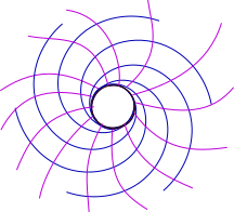
(a)

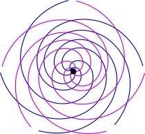
(b)

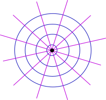
(c)

Figure 2: Configurations with symmetry (a) $\mathbf{SO}(2)$, (b) $\mathbf{O}(2)$ and (c) $\mathbf{O}(2)[\mathbf{SO}(2)]$.

For $\mathbf{SO}(2)$, we choose $p_{1}\equiv p_{2}\equiv p_{3}\equiv 1$ in Table 1, so that the differential form is

$$(1+y^{2}-x^{2}+2xy,x^{2}-y^{2}+2xy,1+x^{2}-y^{2}-2xy).$$

The homomorphism $\lambda$ is trivial and the discriminant function is $\mathbf{O}(2)$-invariant given by

$$\delta(x,y)=2(x^{2}+y^{2})^{2}-1.$$

This is illustrated in Fig. 2(a).

For $\mathbf{O}(2)$, we choose $p_{1}\equiv 0,p_{2}\equiv 1$, so the differential form is

$$(y^{2}-x^{2},2xy,x^{2}-y^{2}).$$

The homomorphism $\lambda$ is such that $\ker\lambda=\mathbf{SO}(2)$ and the discriminant function is $\mathbf{O}(2)$-invariant given by

$$\delta(x,y)=(x^{2}+y^{2})^{2}.$$

This is illustrated in Fig. 2(b).

The configuration in Fig. 2(c) is $\mathbf{O}(2)[\mathbf{SO}(2)]$-symmetric, whose quadratic form has been chosen by taking $p\equiv 1$ in Table 1, that is,

$$(2xy,x^{2}-y^{2},-2xy).$$

The homomorphism $\lambda$ is trivial and the discriminant function is the $\mathbf{O}(2)$-invariant given by

$$\delta(x,y)=(x^{2}+y^{2})^{2}.$$

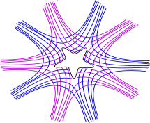
(a)

(b)

Figure 3: Configurations with symmetry group given by (a) $\mathbf{Z}_{5}$ and (b) $\mathbf{Z}_{4}[\mathbf{Z}_{2}]$ .

We now consider $\mathbf{Z}_{5}$ taking $p_{1}\equiv p_{2}\equiv p_{5}\equiv 1$ and $p_{3}\equiv p_{4}\equiv p_{5}\equiv 0$ in Table 1, so that the differential form is

$$(1+y^{2}-x^{2}-3x^{2}y+y^{3},2xy+x^{3}-3xy^{2},1+x^{2}-y^{2}+3x^{2}y-y^{3}).$$

The homomorphism $\lambda$ is necessarily trivial. The discriminant function is the $\mathbf{Z}_{5}$-invariant given by

$$\delta(x,y)=(x^{2}+y^{2})^{3}+10x^{4}y-20x^{2}y^{3}+2y^{5}+(x^{2}+y^{2})^{2}-1.$$

The picture for this case is shown in Fig. 3(a). The star shape of the discriminant set is in fact $\mathbf{Z}_{5}$-symmetric without reflectional symmetries, as it is easily checked by direct calculation.

Fig. 3(b) is a $\mathbf{Z}_{4}[\mathbf{Z}_{2}]$ case, considering $p_{1}\equiv p_{2}\equiv p_{4}\equiv p_{5}\equiv 1$ and $p_{3}\equiv p_{6}\equiv 0$ in Table 1, so that the differential form is

$$(-x^{4}+6x^{2}y^{2}-y^{4}+4x^{3}y-4xy^{3},x^{4}-6x^{2}y^{2}+y^{4}+4x^{3}y-4xy^{3},x^{4}-6x^{2}y^{2}+y^{4}-4x^{3}y+4xy^{3}).$$

The homomorphism $\lambda$ must be such that $\ker\lambda=\mathbf{Z}_{2}.$ The discriminant set is just the origin, given as the zero set of (the $\mathbf{O}(2)$-invariant)

$$\delta(x,y)=2(x^{2}+y^{2})^{4}.$$

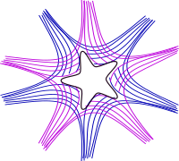
(a)

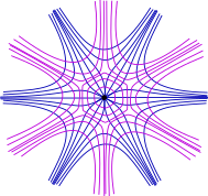
(b)

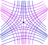
(c)

Figure 4: Configurations with symmetry groups $\mathbf{D}_{5}$, $\mathbf{D}_{6}[\mathbf{Z}_{6}]$ and $\mathbf{D}_{6}[\mathbf{D}_{3}(\kappa_{x})]$.

For $\mathbf{D}_{5}$ in Table 1, we take $p_{1}\equiv p_{2}\equiv p_{3}\equiv 1$, so that the differential form is

$$(1+y^{2}-x^{2}-x^{3}+3xy^{2},2xy-3x^{2}y+y^{3},1-y^{2}+x^{2}+x^{3}-3xy^{2}).$$

In this case, $\ker\lambda=\mathbf{Z}_{5}$ and the discriminant function is the $\mathbf{D}_{5}$-invariant given by

$$\delta(x,y)=(x^{2}+y^{2})^{3}+2x^{5}-20x^{3}y^{2}+10xy^{4}+(x^{2}+y^{2})^{2}-1.$$

This is illustrated in Fig. 4(a).

We now consider $\mathbf{D}_{6}[\mathbf{Z}_{6}]$ choosing $p_{1}\equiv p_{2}\equiv 1$ and $p_{3}\equiv 0$ in Table 1, so that the form is

$$(2xy-4x^{3}y+4xy^{3},x^{2}-y^{2}+x^{4}-6x^{2}y^{2}+y^{4},-2xy+4x^{3}y-4xy^{3}).$$

In this case $\lambda$ is trivial and the discriminant function is $\mathbf{D}_{6}$-invariant and given by

$$\delta(x,y)=(x^{2}+y^{2})^{4}+2x^{6}-30x^{4}y^{2}+30x^{2}y^{4}+2y^{6}+(x^{2}+y^{2})^{2}.$$

The picture is given in Fig. 4(b).

We now turn to $\mathbf{D}_{6}[\mathbf{D}_{3}(\kappa_{x})]$ taking $p_{1}\equiv 1$ and $p_{2}\equiv p_{3}\equiv 0$ in Table 1, so that the form is

$$(-x,-y,x).$$

In this case, $\ker\lambda=\mathbf{D}_{3}(\kappa_{y})$ and the discriminant set is the origin, given by the zero set of

$$\delta(x,y)=x^{2}+y^{2}.$$

The picture is given in Fig. 4(c).

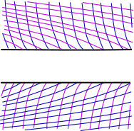
(a)

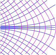
(b)

Figure 5: Configurations with symmetry groups $\mathbf{Z}_{2}$ and $\mathbf{Z}_{2}[{\bf 1}]$.

Consider now $\mathbf{Z}_{2}$ for $p_{1}\equiv p_{2}\equiv p_{3}\equiv 1$ from Table 1, so that the form is

$$(1,y,1).$$

We have $\ker\lambda={\bf 1}$ and the discriminant function is $\mathbf{Z}_{2}$-invariant and given by

$$\delta(x,y)=y^{2}-1.$$

See the illustration of this case in Fig. 5(a).

Fig. 5(b) is a $\mathbf{Z}_{2}[{\bf 1}]$ case, for which we have chosen $p_{1}\equiv p_{2}\equiv 1$ and $p_{3}\equiv-1$ in Table 1 , so that the form is

$$(y,1,-y).$$

The homomorphism $\lambda$ is trivial and the discriminant function is $\mathbf{Z}_{2}$-invariant and given by

$$\delta(x,y)=y^{2}+1.$$

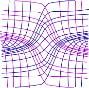
(a)

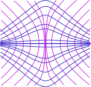
(b)

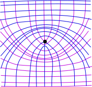
(c)

Figure 6: Configurations with symmetry groups $\mathbf{Z}_{2}\times\mathbf{Z}_{2},\mathbf{Z}_{2}\times\mathbf{Z}_{2}[\mathbf{Z}_{2}(-I)]$ and $\mathbf{Z}_{2}\times\mathbf{Z}_{2}[\mathbf{Z}_{2}(\kappa_{x})]$.

For $\mathbf{Z}_{2}\times\mathbf{Z}_{2}$ in Table 1, we take $p_{1}\equiv p_{2}\equiv 1$ and $p_{3}\equiv-1$, so that the differential form is

$$(-x,-y,x).$$

In this case $\ker\lambda=\mathbf{Z}_{2}$ and the discriminant function is the $\mathbf{Z}_{2}\times\mathbf{Z}_{2}$-invariant given by

$$\delta(x,y)=x^{2}y^{2}+1.$$

This is illustrated in Fig. 6(a).

We now consider $\mathbf{Z}_{2}\times\mathbf{Z}_{2}[\mathbf{Z}_{2}(-I)]$ choosing $p1\equiv p_{2}\equiv 1$ and $p_{3}\equiv-1$ in Table 1, so that the form is

$$(xy,1,-xy).$$

In this case $\lambda$ is trivial and the discriminant function is $\mathbf{Z}_{2}\times\mathbf{Z}_{2}$-invariant and given by

$$\delta(x,y)=x^{2}y^{2}+1.$$

The picture is given in Fig. 6(b).

Finally, consider $\mathbf{Z}_{2}\times\mathbf{Z}_{2}[\mathbf{Z}_{2}(\kappa_{x})]$ taking $p_{1}\equiv 1,p_{2}y^{2}$ and $p_{3}\equiv-1$ in Table 1, so that differential form is

$$(x,y^{3},-x).$$

In this case $\ker\lambda=\mathbf{Z}_{2}(\kappa_{y})$ and the discriminant function is given by

$$\delta(x,y)=x^{2}+y^{6}.$$

See the illustration of this case in Fig. 6(c).

Acknowledgements: Research of P. T. was supported by CAPES Grant 8474758/D.

References

- [1] T. Antoneli, P.H. Baptistelli, A.P.S. Dias, M. Manoel, Invariant theory and reversible-equivariant vector fields, J. Pure Appl. Algebr., 213, (2009), 649-663.
- [2] J.W. Bruce, D. L. Fidal, On binary differential equations and umbilics, Proc. Roy. Soc. Edinburgh Sect. A 111, (1989), no.1-2, 147-168.
- [3] J.W. Bruce, F. Tari, On binary differential equations, Nonlinearity 8, (1995), 255-271.
- [4] J.W. Bruce, F. Tari, Implicit differential equations from the singularity theory viewpoint, singularities and differential equations, Banach Center Publ. 33, (1996), 23-38.
- [5] J. W. Bruce, F. Tari, On the multiplicity of implicit differential equations, J. Diff. Eq. 148, (1998), 122-147.
- [6] L. Dara, Singularités génériques des équations differentielles multiformes, Bull. Soc. Brazil Math , (1975), 95-128.
- [7] M. Field, M. Golubitsky, Symmetry in chaos. A search for pattern in Mathematics, art, and nature. Second edition. (SIAM J. Appl. Math., Philadelphia, PA, 2009).
- [8] R. Garcia, J. Sotomayor, Differential Equations of Classical Geometry, a Qualitative Theory, 27a Coloquio Brasileiro de Matematica, (Rio de Janeiro, 2009).
- [9] T. Golubitsky, I. Stewart, D. Schaeffer, Singularities and Groups in Bifurcation Theory , Vol II, Appl. Math. Sci. 69, (Springer-Verlag, 1984).
- [10] V. Guíñez, Rank two codimention 1 singularities of positive quadratic differential equations, Nonlinearity 10 (1997), 631-654.
- [11] V. Guíñez, Positive quadratic differential forms and foliations with singularities on surfaces, Trans. A.M.S. 309(2) (1998), 477-502.
- [12] C. Gutierrez, V. Guíñez, Positive quadratic differential forms: linearization, finite determinacy and versal unfolding, Ann. Fac. Sci. Toulouse Math 5, (1996), 661-690.
- [13] C. Gutierrez, J. Sotomayor, Lines of curvature, umbilic points and Carathéodory conjecture, Resenhas 3, (1998), 291-322.
- [14] E. Hopf, Differential Geometry in the Large, L.N.M. 1000, (Springer-Verlag, 1979).
- [15] M. Manoel, P. Tempesta, On linear equivariant binary differential equations (2016), preprint.
- [16] J. Sotomayor, C. Gutierrez, Structurally stable configurations of lines of principal curvature, Bif. Erg. Th. Appl. (Dijon 1981), 195-215, Astérisque, (1982), 98-99.
- [17] F. Tari, Pairs of foliations on surfaces, Proc. Real and Complex Singularities, LMS Lecture Notes Series 380 (2010), 305-337.
- [18] F. Tari, Geometric properties of the solutions of implicit differential equations, Discrete Contin. Dyn. Syst. 17 (2007), 349-364.
- [19] F. Tari, Two-parameter families of implicit differential equations, Discrete Contin. Dyn. Syst. 13 (2005), 139-162.