The Shape of Dark Matter Haloes
II. The Galactus HI Modelling & Fitting Tool

Abstract

We present a new HI modelling tool called Galactus. The program has been designed to perform automated fits of disc-galaxy models to observations. It includes a treatment for the self-absorption of the gas. The software has been released into the public domain. We describe the design philosophy and inner workings of the program. After this, we model the face-on galaxy NGC 2403, using both self-absorption and optically thin models, showing that self-absorption occurs even in face-on galaxies. These results are then used to model an edge-on galaxy. It is shown that the maximum surface brightness plateaus seen in Paper I of this series (Peters2015A) are indeed signs of self-absorption. The apparent HI mass of an edge-on galaxy can be drastically lower compared to that same galaxy seen face-on. The Tully-Fisher relation is found to be relatively free from self-absorption issues.

1 Introduction

Modelling of the distribution and kinematics of the neutral hydrogen in galaxies beyond our own, and the most nearby systems M 31 and M 33, took off in the 1970s, with the addition of spectroscopic capability to the Westerbork Synthesis Radio Telescope (Allen1974A). This new tool gave observers sufficient spatial and velocity resolution to resolve the HI structure and kinematics for a large number of galaxies. In edge-on galaxies, it thus became possible to trace the outer envelope of the position-velocity (XV) diagram in order to get the rotation curve of the galaxy (Sancisi1979A). Various strategies for this exist, such as fitting for the peak intensity or fitting a one-dimensional Gaussian with fixed velocity dispersion to the outer edge of the XV-diagram (e.g. Garcia-Ruiz2002A). We refer the reader to OBrien2010B for a detailed treatment on the various methods for deriving the rotation curve from a XV-diagram.

For face-on galaxies, fitting the structure and kinematics was first done by modelling the zeroth and first-moments maps, based on the channel maps in the HI data cube. These gave rise to the famous spider diagrams, in which the iso-velocity contours showed the mean velocity of the gas at each position in the galaxy (Rogstad1971A). With the assumption of a thin disc, it is then possible to measure the rotation of the gas in rings centred on the galaxy. The position angle and inclination could be varied as function of the rings. Assuming a rotation curve, Rogstad1974A used it to model the peculiar velocity field of galaxy M 83, and found the presence of a warp. Bosma1978 improved this by minimizing line of sight velocity residuals for different rotation velocity in order to fit a rotation curve to the data. This method proved quite successful at modelling galaxies. It has been extended by many authors into many software packages (Begeman1987; Schoenmakers1999; Spekkens2007; Krajnovic2006). We refer to Jozsa2007 for a detailed discussion on tilted-ring fitting to velocity fields.

The ever-continuing technological improvements led to ever-higher quality observations, which led to ever-better resolved galaxies, both spatially as well as in velocity. A natural consequence of this was the attempt to model the HI data cube itself. This was first attempted by Irwin1991A; Irwin1993A, who developed the Cubit code. Cubit offers the user parameterized functions, which could be automatically fit to the galaxy. The program has later been expanded to fit more properties of galaxies (Irwin1994A).

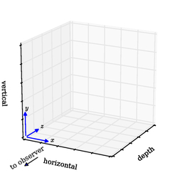
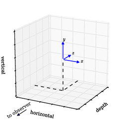
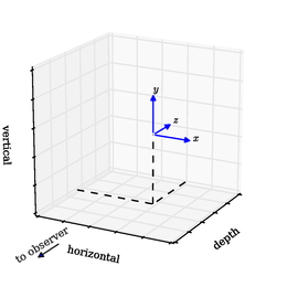
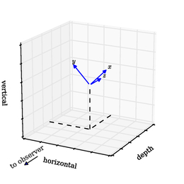
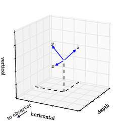
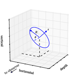
Figure 1: A cartoon illustrating the generation of the galaxy coordinate system. The model demonstrate the generation of an edge-on galaxy at a position angle of $135^{\circ}$. The boxes on each side represent the outer edges of the voxels. From top-left to bottom-right: The initial coordinate system. Centering the coordinate system (Equation 1). The shift parameters can be used to move the central position of the galaxy along the horizontal and vertical axes (Equation 2). The position angle is applied by rotating along the $z$ axis (Equation 3). The inclination is applied by rotating along the $y$ axis (Equation 4). In the final step, we switch to cylindrical coordinates.

Another software package is GALMOD, designed by T.S. van Albada and F.J. Sicking, and incorporated into the GIPSY data reduction system, (GIPSY). Based on a tilted-ring geometry, galmod randomly projects a very large amount of ‘clouds’ in the HI data cube. As these clouds follow the specified kinematics and distribution, after sufficient samples have been drawn, the HI data cube has been built and the only task remaining is scaling the cube to the desired intensity. Galmod does not support automatic fitting and users thus have to fit a cube using the hand-and-eye strategy.

TiRiFiC is another code, which can automate the fit to a cube (Jozsa2007). It is based on a tilted-ring model, but is expanded compared to galmod, to account for inhomogeneity in galaxy discs. Recently, it has used to fit features resembling spiral arms in edge-on galaxies (Kamphuis2013A).

Finally, we note the GalAPAGOS project, which can automatically fit rotation curves in galaxies (Wiegert2011). Out of all software codes currently publicly available, TiRiFiC seems to be the only one under active development. A fully automated three-dimensional fitting routine FAT for Fully Automated TiRiFiC (Kamphuis2015) and another routine, called ^3DBAROLO that also estimates velocity dispersions (Teodoro2015) has become available.

In Paper I (Peters2015A), we presented the HI observations for eight edge-on galaxies. One of the key conclusions of that paper was that self-absorption could well play an important role. The effect of HI self-absorption has long been a topic of concern, for example in the work by Sancisi1979A and of Braun2009. The latter estimated quite significant corrections for self-absorption in the case of the Andromeda Nebula M 31. Yet in most of the publications featuring models of neutral hydrogen in galaxies, the assumption remains that of an optically thin gas.

None of the above software packages supports modelling of self-absorption of the gas. This, combined with some other research questions we had concerning the neutral hydrogen, such as the behavior of the velocity dispersion as function of height above the plane, led us to develop a new tool for generating HI data cubes that could treat for self-absorption. Rather than using a tilted-ring model, we model the galaxy as a single plane on which harmonic offsets above or below the central plane represent the warps. The code was developed in the Python and C++ programming languages, with the computationally most intensive parts implemented as multi-threaded. The software is called Galactus. It has been publicly released under an open-source license and is listed in the Astrophysics Source Code Library as GalactusASCL. The code can be downloaded at sourceforge.net/p/galactus/.

The purpose of this paper is twofold. In Section 2, we present the inner workings of Galactus. Section 3 discusses some important features of the tool in more detail. In Section 4, we explore the effective spin temperature in more detail. We test the program on face-on galaxy NGC 2403 in Section 5, using both an optically thin and a self-absorbing model. In Section 6, the fits from NGC 2403 are projected to an edge-on galaxy to show that the maximum surface brightness profiles seen in Paper I should indeed have been higher. We test how self-absorption can lower the apparent total HI mass, depending on the inclination, in Section 7. The Tully-Fisher relation is shown to be independent of HI self-absorption, in Section 8.

2 Galactus Design

In this section, we discuss how Galactus generates a HI data cube. This generation consists of two steps. In the first phase, the program creates a 3D model of the galaxy, while the second phase performs the radiative transfer.

To generate the model the software creates a three dimensional grid. The first two axes are aligned with, and have the same lengths as, the horizontal and vertical axes of the HI data cube channels. The third axis does not denote velocity, but represents physical depth. The length of the third axis is the same as that of the horizontal axis of the HI data cube.

Each position in this model is a three dimensional pixel, also known as a volumetric pixel, or voxel for short. These voxels all represent a small volume of the galaxy. Since the voxels are perfectly aligned with the HI data cube channels, calculating the brightness of each pixel in a channel can be done by performing the radiative transfer along the depth axis of the voxels associated with that pixel.

Each voxel is assigned coordinates $x$, $y$ and $z$. These are initially aligned with the horizontal, vertical and depth axis. We will subsequently bend and twist these coordinates to match the position and angle of the galaxy as seen in the cube. We emphasise however that these are internal coordinates, the grid of voxels itself does not change and always remains aligned with the HI data cube. The internal coordinates will represent the coordinate system of the galaxy in question.

2.1 Generating the Galaxy Coordinate System

We start with the coordinates $x,y,z$ assigned to the grid of voxels. We first shift the coordinates, such that position (0,0,0) aligns with the centre of the model, i.e.

$$\begin{pmatrix}x\\ y\\ z\end{pmatrix}=\begin{pmatrix}x-\max(x)/2\\ y-\max(y)/2\\ z-\max(z)/2\end{pmatrix}\,\,.$$ (1)

When performing a fit, the actual galaxy is often not perfectly aligned with the centre of the HI data cube. It is thus necessary to shift the coordinates, based on parameters $\mathrm{shift}_{x}$ and $\mathrm{shift}_{y}$,

$$\begin{pmatrix}x\\ y\end{pmatrix}=\begin{pmatrix}x-\mathrm{shift}_{x}\\ y-\mathrm{shift}_{y}\end{pmatrix}\,\,.$$ (2)

Next, the position angle $PA$ is applied. This is done using the coordinate transforms

$$\begin{pmatrix}x\\ y\end{pmatrix}=\begin{pmatrix}x\cos(PA)-y\sin(PA)\\ x\sin(PA)+y\cos(PA)\end{pmatrix}\,\,.$$ (3)

Followed by the inclination $i$,

$$\begin{pmatrix}x\\ z\end{pmatrix}=\begin{pmatrix}x\cos(i)+z\sin(i)\\ -x\sin(i)+z\cos(i)\end{pmatrix}\,\,.$$ (4)

We can now convert to the final cylindrical coordinates system that will be used for the galaxy,

$$\begin{pmatrix}R\\ \theta\\ z\end{pmatrix}=\begin{pmatrix}\sqrt{x^{2}+y^{2}}\\ \arctan(y/x)\\ z\end{pmatrix}\,\,.$$ (5)

Warps are known to exist in many galaxies, yet the actual physics is not well understood. The traditional way of dealing with warps is by applying a tilted-ring model. This is however impossible in our case, as the tilted-ring model does not map all coordinates to a unique physical position. Some voxels would then be mapped to multiple values of $R$ simultaneously, which is undesirable.

We thus choose a different strategy to account for warps. Following Binney1987A, we define a warp as a harmonic oscillation along the disc, in which the mid-plane $z=0$ is raised, or lowered, above the initial mid-plane, as we go around the galaxy following $\theta$. The warp itself has a maximum amplitude which is described by super-function $z_{\mathrm{warp}}(R)$ (see Section 2.6.1), which occurs at pitch angle $\theta_{\mathrm{warp}}$. We do not account for radial changes in pitch angle, so $\theta_{\mathrm{warp}}$ is a single value. Then

$$z=z+z_{\mathrm{warp}}(R)\times\cos(\theta+\theta_{\mathrm{warp}})\,\,.$$ (6)

2.2 Generating the Physics

At this point, we have successfully generated the coordinates for the galaxy. The next step is to calculate the actual physical properties for each voxel. First, the line-of-sight velocity $v_{\mathrm{obs}}$ is calculated, based on rotation velocity $v_{\mathrm{rot}}$ and systemic velocity $v_{\mathrm{sys}}$. The rotation velocity $v_{\mathrm{rot}}$, along with the scale-height of the disc $z_{0}(r)$, velocity dispersion $\sigma(R)$ and face-on surface density $A_{\textrm{{H{}I} }}(R)$ are super-functions, which are prepared by the user (see Section 2.6.1). Then

$$v =v_{\mathrm{rot}}(R)-L\times\!\mid\!z\!\mid\,\,\,\,\,\,\,(v\geq 0),$$ (7)

$$v_{\mathrm{obs}} =v\times\sin(\theta)\times\sin(i)+v_{\mathrm{sys}}\,\,.$$ (8)

Equation 7 offers the possibility to model lagging haloes. The lag is expected to decrease linearly the observed rotation with value $L$ as the height $\mid\!z\!\mid$ above the plane increases. The model automatically prevents $v<0$ and forces these to $v=0$. When no halo lagging is modelled $L$ is set to zero.

The observed velocity dispersion $\sigma$ is calculated separately for the three (cylindrical) directions $\sigma_{z,\mathrm{obs}}$, $\sigma[B_{R,\mathrm{obs}}$ and $\sigma_{\theta,\mathrm{obs}}$, and then combined into a single observed velocity dispersion $\sigma_{\mathrm{obs}}$. The $a_{R},a_{z},a_{\theta}$ components are scalars to account for a possible anisotropic velocity-dispersion tensor. There is currently no known case of anisotropy, so we set $a_{R},a_{z},a_{\theta}$ to one by default. We also correct for instrument broadening using dispersion $\sigma_{\textrm{inst}}$, based on the channel-width $dv$. Then

$$\sigma_{z,\mathrm{obs}} =a_{z}\sigma(r)\times\sin(\theta)\times\sin(i)\,\,,$$ (9)

$$\sigma_{R,\mathrm{obs}} =a_{R}\sigma(r)\times\cos(i)\,\,,$$ (10)

$$\sigma_{\theta,\mathrm{obs}} =a_{\theta}\sigma(r)\times\sin(i)\times\sin(\theta)\,\,,$$ (11)

$$\sigma_{\textrm{inst}} =dv/2.355\,\,,$$ (12)

$$\sigma =\sqrt{\sigma_{z,\mathrm{obs}}^{2}+\sigma_{R,\mathrm{obs}}^{2}+\sigma_{\theta,\mathrm{obs}}^{2}+\sigma_{\textrm{inst}}^{2}}\,\,.$$ (13)

The system takes the face-on surface density $A_{\textrm{{H{}I} }}(R)$ and, using the flaring $z_{0}(R)$, converts it into a mid-plane density $\rho_{\mathrm{m}}(R)$. From this, the actual density $\rho$ for each voxel is calculated. We treat the gas flaring as a Gaussian distribution. There exist alternative distributions, but the Gaussian has some advantages for the analysis of the hydrostatics, in Paper V (Peters2015E). Based on Olling1995A, the errors due to this are expected to be minor. Then

$$\rho_{\mathrm{m}} =\frac{A_{\textrm{{HI}}}(R)}{\sqrt{2\pi z_{0}(R)^{2}}}\,\,,$$ (14)

$$\rho =\rho_{\mathrm{m}}\exp\left[-\frac{z^{2}}{2\,z_{0}(R)^{2}}\right]\,\,.$$ (15)

The densities $\rho$ are all in units of HI atoms per cm³. In the final step, we convert to a local column density $N_{\mathrm{HI}}$ cm^-2 by multiplying with the physical length $ds$ that a single voxel represents along its depth axis.

$$N_{\mathrm{\textrm{{HI}}}}=\rho\,\,ds$$ (16)

2.3 Generating the HI data Cube

We have now prepared the 3D cube and it is time to perform a ray-trace through the voxels along the depth axis and generate the final HI data cubes. Galactus supports two integration modes: optically thin and self-absorption.

2.3.1 Optically thin

We assume that the HI follows a Gaussian velocity distribution,

$$N_{\mathrm{\textrm{{HI}}}}dv=\frac{N_{\mathrm{\textrm{{HI}}}}}{\sqrt{2\pi\sigma^{2}}}\exp\left[-\frac{(v-v_{\mathrm{obs}})^{2}}{2\sigma^{2}}\right]\,\,.$$ (17)

For a single channel in the HI data cube, starting at velocity $v_{1}$ and with a channel width $dv$, the number of atoms $N$ in a voxel that are contributing to the emission in a single channel, can be calculated as

$$N=\int_{v_{1}}^{v_{1}+dv}{N_{\mathrm{\textrm{{HI}}}}\,dv}\,\,.$$ (18)

We solve this integral using the error function erf, i.e.

$$N=\frac{N_{\mathrm{\textrm{{HI}}}}}{2dv}\left[{\rm erf}\left(\frac{v_{1}+dv-v_{\mathrm{obs}}}{\sqrt{2\pi\sigma^{2}}}\right)-{\rm erf}\left(\frac{v_{1}-v_{\mathrm{obs}}}{\sqrt{2\pi\sigma^{2}}}\right)\right]$$ (19)

To calculate the optically thin surface-brightness of each voxel, we use the optically thin limit of the radiative transfer equation (Draine2011, Equation 8.26), i.e.

$$T_{B,\textrm{thin}}=\frac{N}{1.8127\times 10^{18}\,dv}\,\,.$$ (20)

As there is no self-absorption, the intensity of a pixel can simply be calculated by taking the sum of $T_{B}$ in all voxels along the depth axis at the position of that pixel.

2.3.2 Self-absorption

When running in self-absorption mode, the calculation gets more complex. We follow the method from the previous subsection up to equation 20, which gives us the emitted temperature in the velocity range of the channel per voxel for an optically thin model. From this, we can then calculate the optical depth $\tau_{\nu}$ of that voxel as,

$$\tau_{\nu}=T_{B,\textrm{thin}}/T_{\mathrm{spin}}\,\,.$$ (21)

We assume that the galaxy has no internal continuum absorption, nor a background continuum source. This assumption is at least true for the galaxies in Paper I, although it does not hold for every galaxy. To calculate the brightness of a pixel, we begin for the voxel at the back of the depth axis associated with that pixel, and calculate the radiative transfer equation with $T_{\mathrm{bg}}=0$ (Draine2011, Equation 8.22).

$$T_{B,\textrm{self-absorbing}}=T_{\mathrm{bg}}\textrm{e}^{-\tau_{\nu}}+T_{\mathrm{spin}}\left(1-\textrm{e}^{-\tau_{\nu}}\right)$$ (22)

For subsequent voxels $T_{\textrm{bg}}$ is the $T_{B}$ from the previous voxel. We continue this for all voxels along the depth axis until the final value $T_{B}$, which is adopted as the brightness for that pixel.

In our own Galaxy, many lines of sight are optically thick within a few hundred parsec (Allen2012A). To ensure sufficient accuracy, it is therefore advised to choose the physical length of each voxel along the depth axis, such that it does not represent more than a hundred parsec. This can be done using the accuracy parameter (see Section 3.2).

We note that the use of a constant spin temperature $T_{\textrm{spin}}$ and a uniform density $\rho$ per voxel serves only as an approximation. In reality the HI in galaxies consists of gas at a range of spin temperatures, not to mention varying densities (e.g. clouds) on scales much smaller than a hundred parsec. We discuss this in more detail in Section 4.

2.4 Beam Smearing

After the HI data cube has been generated, we convolve the cube with the beam $\theta_{\textrm{FWHM}}$. Note that we require the beam to be circular and the cells to be square.

2.5 Simulating Noise

It is possible to introduce artificial noise into a cube. This can be done using the addition of the -N argument to the command line call to Galactus. The noise $\sigma$ in Table 3 of Paper I was measured as the standard deviation per pixel. In reality however, the noise is correlated between neighbouring pixels due to the beam smearing. Galactus automatically corrects for this, such that the noise $\sigma$ is equal to that as measured from the standard deviation of the convolved field.

2.6 Input

Galactus can be used in two modes, stand-alone and as a software library. To get the stand-alone version, the user can download the source code of the program from the dedicated website at sourceforge.net/p/galactus. After compiling the required C++ libraries, the program can then be run from the program folder using the command ./Galactus ini-file. Galactus uses ini-files as its main source of information, and any run of the program thus needs to be set up using them. We provide a list of all the options in the online Appendix.

It is also possible to import Galactus into your own Python programs as a library. All libraries required to run the program are contained in the support/ module. It is beyond the scope of this paper to discuss this in detail and we refer to the documentation in the code itself for more details. In short, to generate a basic model, a programmer would first need to import the Galaxy class from the support.parameters module, initialise a version of it, and then use the parse_ini(filename) method to initialise all parameters in the Galaxy object. The HI data cube can then be generated by calling the support.mainmodel.model() method. The source code has been extensively documented, and we invite developers to have a look and contribute to the code-base.

2.6.1 Superfunctions

While most variables in Galactus are single valued, the rotation curve and face-on surface density are examples of so-called super-functions. Super-functions are a special class of functions that can behave differently based on the preference of the user. In their 1 or 2 modes, (see Section A) they act as parametrised functions, while in the 3 and 4 modes they act as tabulated functions. In tabulated mode, the user specifies the values of the function that the function has at positions $R$. During runtime, Galactus performs a linear interpolation over these points to calculate the value of intermediate radii. We have experimented with alternative types of interpolation, such as spline interpolation. While favourable from a theoretical point of view, in practise we found that during fitting a spline could start to show extreme spikes (both negative and positive), in an attempt to still reach all the user specified $R$ and $f(R)$ values. This made attaching boundary conditions very hard. In the end, we have settled for linear interpolation between values.

In parametrised mode, the functions are simplified to an analytical form that best fits their common profiles. For example, the velocity curve $v_{\textrm{rot}}$ has a parametrised form of $v_{\textrm{rot}}(R)=a+a/(R/b+1)$. The advantage of parametrizing functions is that it limits the amount of free parameters, in this case only two. The form of each super-function is shown in Table A. Another advantage to parametrised functions is that they are less sensitive to noise – although at the expense of accuracy – and give the ability for a very quick first estimate of the parameters. We provide a function all_to_spline, which can convert parametrised curves to tabulated ones.

2.7 Output

Galactus is capable of producing a range of products, which can be selected in the parameter file. The main output of the program is the generated HI data cube. There are however, more options. In this subsection, we will highlight the most important ones.

2.7.1 Total, visible and hidden matter cube

Since the brightness can depend on opacity, the generated HI data cube no longer represents the total amount of atoms. The total matter cube gives the total amount of atoms in a velocity range, before any self-absorption is applied. This starts with the result of Equation 19, which is a cube with the amount of HI per voxel, for a given channel. Rather than converting the data into temperatures with Equation 20, we instead sum the voxels along the depth axis and thus get the number of atoms. This process is repeated for each channel in the HI data cube.

In contrast, the visible matter cube uses the generated HI data cube and converts it back into atoms, using the inverse of the optically thin approximation from Equation 20. When running in optically thin mode, the visible and total matter cubes are equal. The difference comes into play when running in self-absorption mode. This difference can be visualised with the hidden matter cube, which is a cube showing the difference between the total and visible matter cubes.

2.7.2 Moment maps

Besides channel maps, Galactus can also output various moment maps, specifically the zeroth, first, second and third moments. These follow the same moment definitions as Gipsy (GIPSY).

2.7.3 XV map and integrated profile

Galactus is also capable of plotting the integrated XV (otherwise known as integrated PV) diagrams of the HI data cube, by integrating the generated HI data cube along the vertical axis. By also integrating along the velocity axis, the program can generate an integrated profile.

2.8 Fitting

Fitting a galaxy model to a HI data cube is a very complex problem, and great care needs to be taken in order to fit the data properly. To give the user the best capabilities, we have included a number of fitting routines in the program. Suppose one is fitting a well-resolved face-on galaxy with fixed velocity dispersion and no beam smearing. In this case, a line-of-sight corresponds to a single radius inside the galaxy. This radius is sampled by many pixels as we look around the galaxy. The parameter space is thus very limited, as each radius only has to fit a single face-on surface density and rotation curve. A simple fitting routine, such as the Levenberg-Marquardt algorithm (Press1992), can quickly converge to the optimal solution. We make use of the Scipy package optimise.leastsq.

When beam smearing is involved, the light from various radii starts to overlap, which causes the parameter space to get far more complex. Even worse, local optimal solutions start to appear. For example, where the true face-on surface density at a radius might be $5\times 10^{20}$ atoms/cm², the model could be happily converging towards $3\times 10^{20}$ and $7\times 10^{20}$ atoms/cm² in two adjacent radii, with the beam taking care of the smoothing back to $5\times 10^{20}$ atoms/cm² on average. The velocity dispersion also creates many local optima, especially in edge-on galaxies where the use of a very high velocity dispersion at a high radius $R$ can mask out the velocity dispersion at a slightly lower radius, thus convincing the program that low velocity dispersions at that radius are also acceptable.

To find the global optimum, a more powerful algorithm is required. We have extensively tested many algorithms. Our preferred method is the PSwarm algorithm, which is a combination of pattern search and particle swarm (Vaz07; Vaz09; Thi12) and is used through the OpenOpt framework. Solving for a global optimization problem requires a far more thorough search of the parameter space and thus requires much more time to converge, compared to the Levenberg-Marquardt algorithm. We have also tested various implementations of genetic algorithms, but found that the random nature of the improvements led to unacceptably long convergence times.

We also find that when fitting for the velocity dispersion, it is often misused by an algorithm to ’average over’ local structure in the XV diagram, by using a very high velocity dispersion. This can happen in particular when warps and self-absorption are present, but are not allowed for in the modelling. In those cases, it is not even possible to model the XV diagram accurately. The algorithm will then start to misuse the velocity dispersion.

To estimate the $\chi^{2}$ cost of some parameter set $p$ on the model $T_{\textrm{model}}(p)$, we use least-squares deviations. We show this in Equation 23, where we use the standard deviation of the noise $\sigma$ from the observed HI data cube $T_{\textrm{observation}}$. Index $i$ runs over all pixels in the HI data cube,

$$\chi^{2}(p)=\sum_{i=0}^{N_{\textrm{pixels}}}{\frac{\left[T_{\textrm{model}}(i;p)-T_{\textrm{observation}}(i)\right]^{2}}{\sigma^{2}}}\,\,.$$ (23)

Lastly, we implement a Monte-Carlo Markov-Chain (MCMC) version of the model. MCMC is a different approach to model optimisation. Rather than look for a single parameter set that represents the global optimal solution, MCMC explores the parameter space and draws samples of parameter sets from the region where, based on the probability distribution, the optimum is expected. We make use of the emcee library (emcee), which implements the affine-invariant ensemble sampler proposed by (emcee2). Following the cost function $\chi^{2}$, given in Equation 23, the log-likelihood $\mathcal{L}$ function for a particular parameter-set $p$ is calculated as

$$\mathcal{L}(p) =\log{\left(-\frac{\chi^{2}(p)}{2}\right)}\,\,,$$ (24)

$$=\log{\sum_{i=0}^{N_{\textrm{pixels}}}{-\frac{\left[T_{\textrm{model}}(i;p)-T_{\textrm{observation}}(i)\right]^{2}}{2\sigma^{2}}}}\,\,.$$ (25)

emcee uses multiple MCMC samplers in parallel, each of which generates a chain of samples. For the number of samplers we choose double the amount of free parameters, which for tabulated fitting implies 150-300 chains. After a sufficiently long burn-in period, we collect a large group of $N$ samples from the collection of chains. For each free parameter that is being fitted, the group thus has $N$ values that this parameter would most likely have. These values thus form a distribution. In this and subsequent papers, we make use of the central 68, 95 and 99.7% of the likelihood distribution to denote the errors. Note that if the distribution in a parameter follows a Gaussian distribution, this would be equal to the one, two and three sigma deviations of that Gaussian.

3 Notes

3.1 Masking the Data

Galactus can deal with masked pixels. Pixels that are masked in the input HI data cube, specified with the  textttimage parameter (see also Section A), are treated as pixels with a value of zero. Galactus will still render the corresponding pixels in the output model, as the user could still be interested in the model at these pixels, but has masked them on purpose for some reason.

The mask parameter can be used to specify which pixels Galactus does not need to render. The parameter needs to point to a HI data cube, which can be the same as the one used in the image parameter. All pixels in the channel maps that make up the HI data-cube that have value NaN are selected as the masked pixels. Galactus calculates which voxels contribute to which pixels. If a voxel only contributes to masked pixels, it is removed from the calculation. This can lead to drastic performance increases.

The last type of mask is the boundaries mask. This can be used to specify in which channel maps the line-of-nodes velocity $v_{\textrm{rot}}(R)$ is expected to lie. It is then possible to mask everything except the outer envelope of a XV diagram. The fitting algorithms are then constrained in the $v_{\textrm{rot}}(R)$ parameter.

3.2 Concerning the Resolution

By default, Galactus traces only one ray per pixel. The initial cube has voxels that are one pixel wide on all sides. Thus, if the output cube has pixels with a (projected) size of one kpc, the voxels are one kpc on each side as well, and the ray is thus sampled every one kpc as it crosses the galaxy. For a galaxy that has a diameter of 20 kpc, the rays will thus at most only sample 20 positions inside the galaxy. This can lead to a jagged looking result.

To provide a better representation of the galaxy, we have introduced two additional user options. The first is the accuracy level, which controls the number of samples along the ray. It works as a scalar on the original number of samples along the depth axis, such that if one originally measured 20 samples, an accuracy level of four would lead to 80 samples. Following the above example, these would thus be separated 250 pc apart along the ray.

The second option is super-sampling, a technique common in the 3D graphics industry. In super-sampling, each output pixel is represented by multiple rays at slightly different positions inside the pixel, with the result being the average of all rays. For example, suppose the original ray runs a trace centred on the middle of the pixel, thus at position 1/2. Then with super-sampling, we have two rays, both at 1/3 and 2/3. Suppose that a significant change would beyond position 1/2. The normal model would not represent this, while super-sampled pixel would. Super-sampling works in both the horizontal and vertical directions. A super-sampling of factor two means each pixel is sampled by four rays.

An increased accuracy thus increases the number of voxels along the depth axis. An increase in super-sampling decreases the size of an individual voxel along the horizontal and vertical axis and thus increases the number of voxels quadratically. The increases in accuracy and super-sampling are thus increases in the number of voxels that need to be calculated, which come with a performance penalty. It is thus important to realise that there is a trade-off between the desired accuracy and the time available.

In Figure 2, we visualise this trade-off. Shown are the timing results of an edge-on model, at multiple combinations of super-sampling and accuracy levels, with their relative error compared to a very high-resolution model with an accuracy of five and a super-sampling of five, which in this case implies a model with voxels that each represent 27 pc on all side. In a perfect world, the accuracy and super-sampling could be set to $\infty$ and the results would be perfect. In practice however, due to time constraints, there is no single right setting, it is thus important to think about the problem and decide what the best setting should be. For example, in a face-on galaxy one quickly runs the risk of ’overshooting’ the disc, if there were not enough samples along the ray, and a higher accuracy would then be desirable. In an edge-on, overshooting the disc is less important, but one might want to super-sample the galaxy as to model the vertical structure more accurately.

A super-sampling of two incorporates a special feature, which positions the four rays in an optimal distribution. In this way, both the horizontal and vertical axis of the pixel in question are traced at four unique positions, rather than the default of two positions per axis. The effect of this can be seen in Figure 2, where the results from a super-sampling of 2 are nearly equal to the far more computationally expensive super-sampling of four (i.e. 16 rays). A super-sampling of two outperforms a super-sampling of three. Figure 2 also demonstrates that increasing the accuracy does not drastically improve the model. We recommend that the accuracy be chosen such that the length of the voxel along the depth axis is at most 100 parsec, such that the radiative transfer equation is calculated with sufficient precision.

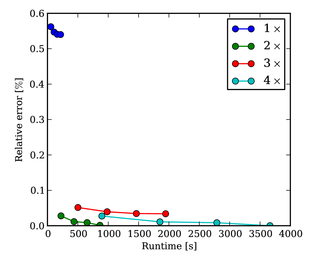
Figure 2: The accuracy versus time trade-off visualized. The various tracks show the various super-sampling modes, while the dots along each track represent the accuracy level used. Along each track, the top left point is always accuracy level of one, progressing to an accuracy level of four, at the right-hand side. Overall the rule holds that the closer to (0,0), the better.

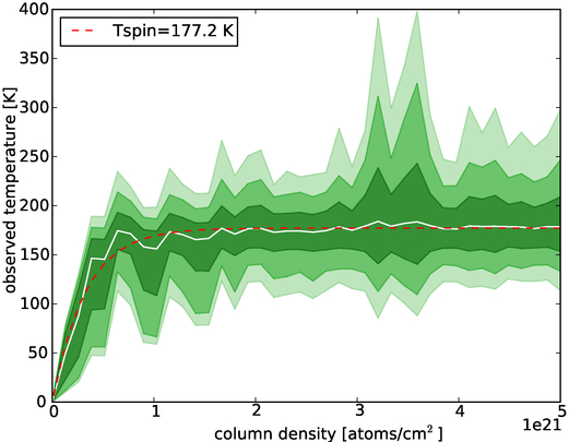
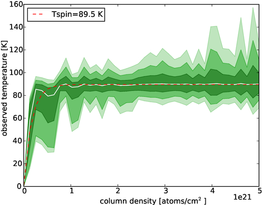
Figure 3: Effective spin temperature assuming $40\%$ (left panel) or $80\%$ (right panel) of the gas is in the CNM. Colour bars represent $68.5\%$, $95.45\%$ and $99.73\%$ of the distribution at each point. In white the $50\%$ (median) of the sample is shown. The red dashed line represents the fitted effective spin temperature.

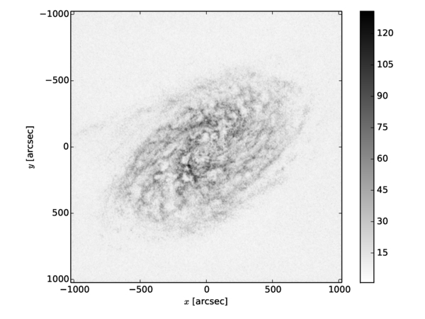
Figure 4: Maximum surface brightness map for NGC 2403. The values for the bar on the right is brightness temperature in Kelvin.

4 The Effective Spin Temperature

In a real galaxy, the HI never has a single spin temperature. The gas is balanced between the phases of the CNM, which has a median spin temperature of 80 K and the WNM, with temperatures between 6000 and 10000 K. The fraction of the mass contained in either state remains unclear, but it was estimated that $40\%$ of the neutral hydrogen mass of the Galaxy is in the CNM (Draine2011).

With such a wide range in temperatures, how reliable is the use of a single effective spin temperature? To test this, we have run a range of Monte Carlo simulations. For a fixed CNM fraction $p$, we calculate the effective spin temperature over a range of column densities. For column density $N_{\textrm{{H{}I} }}$, we divide it up in $N_{\textrm{clouds}}$ equal sized bins, each of which represents a cloud of gas with a column density $N_{\textrm{cloud}}$. The number of clouds is randomly picked between 100 and 1000, to represent the variation in crossing a real galaxy. Based on fraction $p$, we randomly choose if a cloud is part of either the CNM or the WNM. If it is a CNM cloud, it is assigned a random spin temperature $T_{\textrm{spin}}$, chosen from a uniform distribution between 50 and 100 K. Otherwise, it is assigned a $T_{\textrm{spin}}$ chosen from a distribution between 6000 and 8000 K. We then perform a line-of-sight integration, starting with background temperature $T_{\textrm{bg}}=0$ K, using Equations 20, 21 and 22.

Taking 1000 samples at each column density $N_{\textrm{{HI}}}$, we get a distribution of observed temperatures $T_{B}$. We show the results for two mass fractions in Figures 3a and 3b. We fit a single effective $T_{\textrm{spin}}$ to the median of the distributions, using

$$T=T_{\textrm{spin}}\left(1-e^{-\tau}\right)\,\,.$$ (26)

The results are over-plotted in red in Figures 3a and 3b. For the $40\%$ fraction, we find an effective spin temperature of 177.2 K, while for the $80\%$ fraction we find 89.5 K. Clearly, the balance between the two populations is important. More importantly, in both cases we see that the median spin temperature levels out, and a single effective spin temperature gives a decent fit to the median one. Provided the right value is chosen, it is thus possible to use a single effective spin temperature when modelling a galaxy. What the exact value for this effective spin temperature is, is hard to determine and is beyond the scope of this work. During fitting, we shall use a spin temperature of 100 K, a value in good agreement with the figures in Paper I.

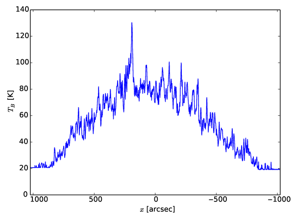
Figure 5: Radial maximum surface brightness of NGC 2403

5 Face-on Galaxy NGC 2403

In the following sections we test the program for a number of cases. To begin with, we wish to test our fitting routines on a face-on galaxy to confirm the accuracy of the rotation curve and surface density modelling. For this purpose, we have chosen the galaxy NGC 2403. Like the galaxies in our sample it is a nearby, late-type Scd galaxy (Tully2000A). HI observations of high spatial and velocity resolution are available for it. Even though the rotation velocity is slight higher (130 versus on average 90km s^-1) it is suitable for comparing to our sample of edge-on, late-type galaxies (Paper I). Using the tip of the red giant branch, Dalcanton2009A estimated the distance at 3.2 Mpc. The HI kinematics have have been studied in detail by Sicking1997A, Fraternali2001A; Fraternali2002A and DeBlok2008A. The galaxy is part of the public-data release from The HI Nearby Galaxy Survey (THINGS), which was based on B-, C- and D- configuration Very Large Array (VLA) observations (Walter2008A). The THINGS observations were previously studied in detail by DeBlok2008A, who measured a systemic velocity $v_{\mathrm{sys}}$ of 132.8 km s^-1 and an inclination $i$ of $62.9^{\circ}$.

We test Galactus using the naturally weighted HI data cube from the THINGS website. The original cube has a size of $2048\times 2048$ pixels and 61 channels, which is too large for Galactus to handle. Miriad task smooth was used to create a circular beam with a full-width half-maximum of 12.4  arcseconds. We used the task regrid to downsize the resolution from 1.0 to 8.8 arcsec/pixel, resulting in somewhat less than 2 pixels/beam. The initial beam was $8.75\times 7.65$ arcsec, with a position angle of 25.2 degrees. We used the task regrid to downsize the sampling of the data from 1.0 to 8.8 arcsec/pixel, resulting in somewhat less than 2 pixels/beam. We have chosen this sampling as this corresponds to roughly 100 parsec per pixel. As each pixel is supersampled by 4 rays, the area of the FWHM of the beam will be modeled by of order 20 rays, which is sufficient to prevent undersampling. While an even higher resolution would have been desirable, it was found to be computationally infeasable, as the required memory and computation time increase with the power 3. Using task cgcurs, a mask was drawn by hand around all regions containing flux. With task imsub, we used this mask to create a final, masked cube that only contains parts of the cube where flux was detected. The final cube has a size of $232\times 228$ pixels and 55 channels at 5.169 km s^-1 resolution.

In Figure 4, the maximum surface brightness has been calculated from the original THINGS image. Here we have converted the intensity $I$ from Jy/beam to Kelvin using Equation 4 of Paper I:

$$T_{B}=\frac{\lambda^{2}S}{2k_{B}\Omega}=\frac{606000S}{\theta^{2}}\,\,..$$ (27)

A clear spiral structure is visible in the figure. Most of the brightness hovers between 45 and 60 K and appears as spiral arm structure, with local regions peaking at over 120 K. We rotated the galaxy such that the major axis is lined up with the horizontal x-axis. If we only look at the maximum brightness along the horizontal axis, such that each position reflects the maximum brightness independent of location along vertical axis, we get the result as seen in Figure 5. This produces a result similar to the maxima along the major axis in edge-on galaxies as seen in Paper I. There we found a plateau around 80 Kelvin in all edge-on galaxies for a significant part of their discs. There is no clear plateau in Figure 5. The wings of this profile are much extended, running continuously towards the background. This is different compared to our edge-on galaxies, where we observed very sharp wings. In Paper I, we argued that the plateau in the profile was due to self-absorption in long lines-of-sight. The shorter lines-of-sight in NGC 2403 would therefore not be expected to exhibit (strong) signs of self-absorption. Only in the dense inner region do the densities still reach levels high enough for self-absorption to significantly affect them, as exhibited by the peak around 80 K. We thus argue that with the exception of the central part, most of the galaxy is not affected by significant self-absorption. We note in general, that observations of self-absorption can only occur when the beam has sufficient spatial resolution. Otherwise, the effect will wash out due to smearing.

We fit NGC 2403 using both an optically thin model and a self-absorption model. For the self-absorption model, we use a spin temperature $T_{\mathrm{spin}}$ of 100 K. We fit the galaxy using a constant velocity dispersion of 10 km/s. We constrain the disc to a thickness of 700 pc in the inner part and flaring out to 1 kpc at 1400” ($23$ kpc). Warps or lagging haloes are beyond the scope of the current test. A double-pass strategy is used to fit the data. We first use the parametrised functions for the face-on surface density, flaring and rotation curve. This pass is fitted using the Levenberg-Marquardt algorithm. After that, we interpolate over the fitted functions and tabulate them into 37 chunks with a separation of 38”. We then run a second pass. As the galaxy is face-on and very well resolved there is no strong danger of running into local minima, and we thus again use the quick Levenberg-Marquardt algorithm.

The results for this fitting are shown in Figure 6. The rotation curves of the optically thin and self-absorbing fits are effectively identical. It is reassuring to find that in both cases the same rotation curve is found, proving that the observed $v_{\textrm{rot}}$ in face-on galaxies is not affected by self-absorption. The profile also matches up well with the profile from Sicking1997A. Only in the outer radii do we suffer more from signal to noise issues. Given the detailed tilted ring and warp fitted by Sicking1997A, which we are ignoring, this is expected.

Now consider the mass models. Unsurprisingly, the optically thin profile is clearly lower than the optically thick profile. The first has a total mass of $2.9\times 10^{9}$ M_⊙. The self-absorbing mass totals at $3.2\times 10^{9}$ M_⊙, of which $\sim 10\%$ is hidden by the self-absorption. The overall shape of the profiles agree well, with all local features visible in both profiles. In comparison, Sicking1997A found slightly more mass than our optically thin model. They report a total mass of $3.27\times 10^{9}$ solar masses for NGC 2403.

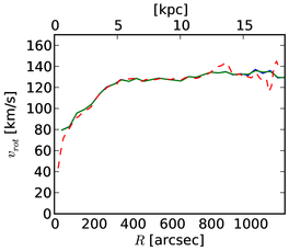
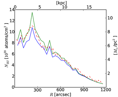
Figure 6: Kinematic and mass models for NGC 2403. The blue profiles represent the optically thin model. The green profiles are the self-absorption fit. The dashed red profiles represent the data from Sicking1997A.

6 The Maximum Surface Brightness in an Edge-on Galaxy

In Section 3 of Paper I, we presented a simple toy model to demonstrate that a plateau of constant maximum surface brightness is an indication of self-absorption. Using Galactus, we can now extend this toy model to a more physical basis. We project the previous fit of NGC 2403 to a full edge-on orientation. We use the self-absorption fit as the face-on surface-density and rotation curves as input parameters (see Figure 6). We will compare between an optically thin model and a self-absorption run at a spin temperature of 100 K.

The results for this test are shown in Figure 7. The model for the galaxy at its original inclination peaks at roughly 40 K (blue line). This is lower than the observed maximum brightness maps as seen in Figure 5. This is expected, as the model cannot recreate the small-scale bright regions seen in the actual observation. When we rotate the galaxy to full edge-on, we see that the long lines-of-sight carry the integration well above 300 K (green line). Especially near the inner part at $x=0$ the model keeps rising. As we have argued in Paper I, this is never observed. Comparing this to the self-absorption model at $T_{\mathrm{spin}}=100$ K, we see that the maximum surface brightness shows a clear plateau around 80 Kelvin with sharp edges. Comparing this to the galaxy observations in Paper I, the self-absorption clearly matches the data better than the optically thin model. Compared to the toy model from Section 3 of Paper I, the result is less dramatic than in Figure 2 in that paper, where we applied a far higher face-on column density distribution than used here.

7 Effect of Inclination on the Visible Mass

Having established that an edge-on galaxy can easily hide a considerable fraction of its neutral hydrogen, we wish to test the relation between inclination and self-absorption. We test the effect of self-absorption on galaxies in the range of inclinations from 60 to 90 degrees. We have selected $T_{\mathrm{spin}}=100$ K and $T_{\mathrm{spin}}=150$ K as the spin temperatures we wish to model, and will produce an optically thin model at each inclination to compare. We use the self-absorption results of NGC 2403 from Section 5 as the basis for all three models.

The results for this fit are shown in Figure 8. It is clear that in both cases self-absorption is present at all inclinations. However, beyond an inclination of about 82 degrees, the effects starts to increase drastically. Similar to Paper I, we find that for a spin temperature of 100 K that $30\%$ of the HI remains undetected. The milder case of a spin temperature of 150 K still has a significant absorption, with $\sim 23\%$ of the HI going unseen.

A natural prediction from Figure 8 would be that in a statistical study the edge-on galaxies would have a lower average HI mass than the face-on to moderately inclined galaxies. We have tried to investigate this by comparing the K-band magnitude (which is expected not to be much affected by inclination effects) with the apparent HI mass, using a combination of literature surveys. Unfortunately, we were unable to confirm or disprove the results, as there were too few edge-on galaxies in the available surveys with exact inclination measured. It is beyond the scope of this project to investigate this in more detail.

8 The Baryonic Tully-Fisher Relation

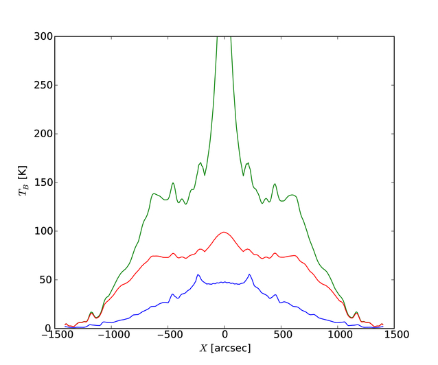
Figure 7: Maximum surface brightness along the major axis based on modelling for NGC 2403. The lower blue line is the galaxy at its normal inclination. The top green line is the optically thin case as seen edge-on. The middle red line is the self-absorption case with a spin temperature of 100 K.

Having established that edge-on galaxies can be affected by significant HI self-absorption, what is the effect on the baryonic Tully-Fisher (TF) relationship? The TF relation relates the dynamical mass of a galaxy to its luminosity and provides a test of theories of galaxy formation and evolution (Verheijen1997A; Bell2001A). We use the two edge-on models from Section 6 as a basis for this analysis. The integrated spectra are shown in Figure 9. The T-F relation is based on the width $w_{20}$ of the profile at 20% of the maximum in the integrated spectra (Tully1977A). Clearly, this height varies drastically between the two cases, yet the difference between the two $w_{20}$ measurements is minimal. This is due to the sharp drop-off that both profiles show at the extremes, where self-absorption is less important. For the optically thin case a value of 285.0 km/s is found and for the self-absorption case 291.0 km/s, an increase of only $2\%$. We thus conclude the $w_{20}$ parameter is not affected significantly by self-absorption.

The baryonic TF relation is however also based on the total baryonic mass $M_{\textrm{bar}}$, and as Figure 9 clearly illustrates, self-absorption can significantly affect that property. The TF-relation has not been well set, with various authors finding slopes between $M_{\textrm{bar}}\propto V^{3}$ and $M_{\textrm{bar}}\propto V^{4}$ (kf11 and references therein). Although beyond the scope of this project, it will be interesting to see if the intrinsic scatter of the T-F relation decreases when self-absorption of the HI is taken into account.

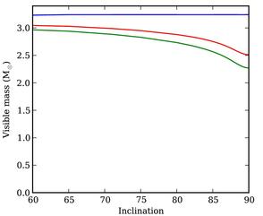
Figure 8: Visible HI in an edge-on model based on NGC 2403. The top blue line is the galaxy as if there is no self-absorption present. The bottom green line has self-absorption at $T_{\mathrm{spin}}=100$ K. The middle red line is the self-absorption at $T_{\mathrm{spin}}=150$ K.

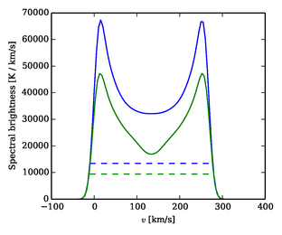
Figure 9: Impact on the width $w_{20}$ as measured from the spectra from an edge-on galaxy affected by in an optically thin (top, blue) and self-absorption with $T_{\textrm{spin}}=100$ K (bottom, green) case.

Appendix A Overview of Input File Layout and Settings

Galactus uses ini-files as input. Each ini-file is divided into various segments that detail the various parts of the program.

[cube

]

image

A list of the filenames to which we are fitting.
Example: ["galaxies/UGC7321.fits.gz"].

name

The name of the object. All output files will have this as a base-name. Example: UGC7321.

comparison

Used for comparing to other ini files. The parameters from this file are also over-plotted in the output profiles. Example: galaxies/UGC7321.ini.

mask

Use a blanking mask in which all pixels of value NaN are ignored. This will speed up the program and changes which pixels are used while fitting. Example: galaxies/UGC7321.fits.gz

boundaries

This file controls which boundaries the rotation curve fitting has to oblige to. Setting parts of this cube to nan will ensure that the $v_{\textrm{rot}}$ will avoid that position.
Example: galaxies/UGC7321.fits.gz

cell

Size of each pixel in arcsec. Galactus requires the pixels to be square. Example: 3.26.

v_cube_min

Velocity of the first channel in km/s. Example: 1565.0.

v_cube_N

Number of channels in the cube. Example: 75.

v_cube_delta

Channel width and spacing, in km/s. Example: 3.298

width

Length of the horizontal axis of the cube, in pixels.
Example: 80.

height

Length of the vertical axis of the cube, in pixels. Example: 25.

halforwhole

Lets the program know if we are modelling the full cube or one side. This sets the length of the depth axis. Example: whole.

[physical]

shift_x

Offset from the centre of the galaxy, compared to the centre of the radio channel, along the horizontal axis, in pixels. Example: 0.

shift_y

Offset from the centre of the galaxy, compared to the centre of the radio channel, along the vertical axis, in pixels. Example: -0.2.

shift_x_free

. Do we have to fit for the shift_x parameter?
Example: yes.

shift_y_free

. Do we have to fit for the shift_y parameter?
Example: no.

v_sys

Systemic velocity of the galaxy, $v_{\textrm{sys}}$, in km/s. Example: 409.3.

v_sys_free

Fit for the systemic velocity? Example: yes.

v_sys_bounds

Tuple with the boundaries between which $v_{\textrm{sys}}$ should be, in km/s. Example: (390.0, 420.0).

distance

Distance $D$ of the galaxy in Mpc. Example: 10.0.

distance_free

Fit for the distance of the galaxy? Note that this is often not a recommended strategy. Example: no.

distance_bounds

Tuple with the boundaries between which the distance $D$ should be found, in Mpc. Example: (9.6, 10.4)

T_spin

Spin temperature of the galaxy. Currently only global spin temperatures are supported. Select None for optically thin. Otherwise, the user can give a positive value, which will be taken as the spin temperature in Kelvin.

rotationcurve_function

Which rotation-curve super-function should be used? Select 1 or 2 when using function $v_{\textrm{rot}}(R)=a+a/(R/b+1)$, where 1 select no-fitting and 2 selects fitting. Selecting 3 or 4 sets for tabulated interpolation, with 3 for no fitting or 4 for fitting.

rotationcurve_x

Either an empty list (e.g. []) when
rotationcurve_function is 1 or 2. Otherwise, a list of positions (expressed in pixels) along $R$, example: [0,1,2,3,4,5]. When 0 is omitted, the program assumes $R=0$ will give a $v_{\textrm{rot}}(R=0)=0$.

rotationcurve_y

Either a two-values list (e.g. [$A$,$B$]) when
rotationcurve_function is 1 or 2. Otherwise a list of rotation curve strengths $v_{\textrm{rot}}$ (expressed in km/s) along $R$, example: [10, 20, 40, 80, 90].

surfacedensity_function

Which face-on-surface-density super-function should be used? Select 1 or 2 when using function $A_{\textrm{{HI}}}(R)=|a|+bR+cR^{2}$, where 1 select no-fitting and 2 selects fitting. Selecting 3 or 4 sets for tabulated interpolation, with 3 for no fitting or 4 for fitting.

surfacedensity_x

Either an empty list (e.g. []) when
surfacedensity_function is 1 or 2. Otherwise a list of positions (expressed in pixels) along $R$, example: [0,1,2,3,4,5].

surfacedensity_y

Either a three-value list (e.g. [$a$,$b$,$c$]) when
surfacedensity_function is 1 or 2. Otherwise a list of face-on surface densities $A_{\textrm{{HI}}}$ (expressed in $10^{20}$ atoms/cm²) along $R$, example: [5,4,2,1,0].

flaring_function

Which flaring super-function should be used? Select 1 or 2 when using function $z_{0}(R)=|a|+|b|R$, where 1 select no-fitting and 2 selects fitting. Selecting 3 or 4 sets for tabulated interpolation, with 3 for no fitting or 4 for fitting.

flaring_x

Either an empty list (e.g. []) when flaring_function is 1 or 2. Otherwise a list of positions (expressed in pixels) along $R$, example: [0,1,2,3,4,5].

flaring_y

Either a two-values list (e.g. [$a$,$b$]) when flaring_function is 1 or 2. Otherwise a list of flaring $z_{0}$ strengths, expressed in pixels, along $R$, example: [1,1,1.1,1.2,1.4].

velocitydispersion_function

Which velocity dispersion super-function should be used? Select 1 or 2 when using function $\sigma(R)=|a|$, where 1 select no-fitting and 2 selects fitting. Selecting 3 or 4 sets for tabulated interpolation, with 3 for no fitting or 4 for fitting.

velocitydispersion_x

Either an empty list (e.g. []) when
velocitydispersion_function is 1 or 2. Otherwise a list of positions (expressed in pixels) along $R$, example: [0,1,2,3,4,5].

velocitydispersion_y

Either a one-value list (e.g. [$a$]) when
velocitydispersion_function is 1 or 2. Otherwise a list of velocity dispersion $\sigma$ strengths, expressed in km/s, along $R$, example: [10,9,8,7,6].

inclination_function

Either 1 for fixed inclination or 2 for fitting.

inclination_value

Value of the inclination $i$, in degrees. Example: 0.0.

inclination_bounds

Tuple with boundary values for the inclination fitting, in degrees. Example: (80.0, 90.0).

PA_function

Either 1 for fixed position angle or 2 for fitting.

PA_value

Value of the position angle, in degrees. Example: 0.0.

PA_bounds

Tuple with boundary values for the position angle fitting, in degrees. Example: (-10, 10).

halolag_function

Either 1 for fixed halo lag or 2 for fitting.

halolag_value

Strength of the halo lag, in km/s per pixel. Example: 0.2.

halolag_bounds

Tuple with boundary values for the halo lag fitting, km/s per pixel. Example: (0,10).

warp_function

Either 3 for fixed warp or 4 for fitting.

warp_theta

Pitch angle for the warp, in degrees. A pitch angle of $0^{\circ}$ represents a line-of-sight warp. Example: 0.0.

warp_theta_bounds

Tuple with the boundaries on the pitch angle of the warp, for fitting, in degrees. Example: (-1.0, 70).

warp_r

List of position along $R$ where to interpolate. In pixels. Example: [0, 20, 400].

warp_r_bounds

List of tuples with the boundaries on the values of warp_r for fitting, in pixels. Example: [(0.0,0.01), (15,40), (400,400.01)].

warp_z

List of offsets from the central plane, in pixels. Example: [0, 0, 0].

warp_z_bounds

List of tuples with the boundaries on the values of warp_z for fitting, in pixels. Example: [(0.0,0.0), (0.0,0.0), (0.0,500)].

dispersiontensor

The values of the velocity dispersion tensor. Example: [1,1,1].

dispersiontensor_free

Do you want the dispersion tensor to be fitted. Not well supported. Example: no.

beam

List with beamsizes in arcsec. Should have the same length as image. Example: [10].

noise

List with the one-sigma noise levels in each cube given by image in Kelvin. Example: [0.79].

[integrator]

intermediate_results

Plot intermediate results during fitting? Example: yes.

accuracy

Accuracy level of the model. Example: 1.

supersampling

Super-sampling level of the model. Example: 2.

[output]

radius_rotationcurve

Plot the rotationcurve $v_{\textrm{rot}}(R)$? Example: yes.

radius_surfacedensity

Plot the face-on surface density $A_{\textrm{{HI}}}(R)$? Example: no.

radius_flaring

Plot the flaring $z_{0}(R)$? Example: yes.

radius_velocitydispersion

Plot the velocity dispersion $\sigma(R)$?
Example: yes.

XV_map

Plot an integrated PV diagram of the data? Example: no.

radius_scale

Controls in which units the radius $R$ is expressed in the previous plots. Options are arcsec, kpc or pixels.

integratedprofile

Plot an integrated profile of the data? Example: yes.

moment0

Plot a zeroth moment map? Example: no.

moment1

Plot a first moment map? Example: no.

moment2

Plot a second moment map? Example: yes.

moment3

Plot a third moment map? Example: no.

cube_visible

Save the final HI data cube, expressed in $10^{20}$ atoms/cm². Example: yes.

cube_total

Save the HI data cube as if it was optically thin, expressed in $10^{20}$ atoms/cm². Example: yes.

cube_missing

Save a cube in which only the hidden atoms are shown, expressed in $10^{20}$ atoms/cm². Example: yes.

cube_opacity

Save the final HI data cube, expressed in the opacity $\tau$. Example: yes.

cube_intensity

Save the final HI data cube, expressed in Kelvin. Example: yes.