$\text{T}\bar{\text{T}}$-deformed 2D Quantum Field Theories

Abstract:

It was noticed many years ago, in the framework of massless RG flows, that the irrelevant composite operator $\text{T}\bar{\text{T}}$, built with the components of the energy-momentum tensor, enjoys very special properties in 2D quantum field theories, and can be regarded as a peculiar kind of integrable perturbation. Novel interesting features of this operator have recently emerged from the study of effective string theory models.

In this paper we study further properties of this distinguished perturbation. We discuss how it affects the energy levels and one-point functions of a general 2D QFT in finite volume through a surprising relation with a simple hydrodynamic equation. In the case of the perturbation of CFTs, adapting a result by Lüscher and Weisz we give a compact expression for the partition function on a finite-length cylinder and make a connection with the exact $g$-function method. We argue that, at the classical level, the deformation naturally maps the action of $N$ massless free bosons into the Nambu-Goto action in static gauge, in $N+2$ target space dimensions, and we briefly discuss a possible interpretation of this result in the context of effective string models.

1 Introduction

The study of integrable models has a long history scattered with many significant achievements, including a deeper understanding of phase transitions and other non-perturbative properties of interacting statistical mechanical systems, the study of important low dimensional condensed matter models [1, 2, 3], and the link with gauge theories in two, three and four space-time dimensions and with the AdS/CFT correspondence [4].

The discovery of a connection between the exact S-matrix method, the Thermodynamic Bethe Ansatz (TBA) [5] and the effective string theory description of the chromoelectric flux tube in confining gauge theories is a further surprising result recently obtained within the integrable model setup [6, 7]. In particular, it has been discovered that the finite-size spectrum of a theory of free massless bosons modified by the inclusion of a very simple scalar scattering phase (CDD factor) can be computed exactly with the TBA method and that its analytic form is precisely the well-known expressions for the energy levels of the Nambu-Goto model obtained in the early days of string theory via covariant quantization [8]. This idea was readily adapted in [9] to encompass the open string case, a framework more directly relevant to the study of the quark-anti-quark potential. In the same paper, the setup was generalised to describe the deformation, via the same CDD factor, of an arbitrary 2D conformal field theory (CFT). A tight link was observed to previous studies on massless RG flows with leading IR attracting operator given by the $\text{T}\bar{\text{T}}$ composite operator built with the chiral and anti-chiral components of the CFT stress-energy tensor (see [10],[11],[12], [13], [14]). Earlier observations on the special rôle played by the $\text{T}\bar{\text{T}}$ operator in integrable perturbations of CFTs were recorded in a few occasions, mainly in the framework of Form Factors [15, 16] for correlation functions, and hints on possible links with CDD factors and TBA may be envisaged in [17]. A general quantum field theory definition of this special composite operator away from criticality was proposed by Sasha Zamolochikov in [18], a paper of central importance for the purposes of the current work. In the context of relativistic integrable field theories with factorised scattering [19], the irrelevant perturbations considered in this paper are described by formally modifying the S-matrix with an extra diagonal phase shift, depending on a deformation parameter $t$:

$$S_{ij}^{kl}(\theta)\rightarrow S_{ij}^{kl}(\theta)\,e^{i\delta^{(t)}_{ij}(\theta)},$$ (1)

where $\theta=\theta_{i}-\theta_{j}$ denote the relative particles’ rapidity and

$$\delta^{(t)}_{ij}(\theta)=\delta^{(t)}(m_{i},m_{j},\theta)=t\,m_{i}m_{j}\,\sinh(\theta).$$ (2)

When the masses of all physical particles are sent to zero, the net effect of the presence of the CDD factor is to introduce an interaction between left and right-moving massless excitations. The phase shift for this process is simply

$$\delta_{ij}^{(t)}(\theta_{i}-\theta_{j})=t\,\frac{M_{i}M_{j}}{2}\,e^{\theta_{i}-\theta_{j}}=-2t\,p^{(+)}_{i}\,p^{(-)}_{j},$$ (3)

where $p^{(+)}_{i}$ and $p^{(-)}_{j}$ are the momenta of right and left moving particles, respectively, and $M_{i}$, $M_{j}$ fix the relative energy scales. The CDD factor (2) was introduced in [20] as a generalization of the proposal of [6] to theories with more than one particle species. It was first pointed out in [9] that this deformation corresponds to perturbing the CFT theory with a series of irrelevant operators whose leading term is $\text{T}\bar{\text{T}}$. As we shall discuss in this paper, the introduction of the phase factor in the nonlinear integral equations describing the spectrum at finite-size leads to a characteristic deformation of the energy levels as $t$ is varied, which flows according to the inviscid Burgers equation of hydrodynamics. Further, the wave-breaking phenomenon, typical of the solutions to this simple fluid equation, is seen to correspond to the appearance of a spectral singularity at physical values of the system size: the famous tachyon singularity of effective string theories. While the specific form of the deformation of the spectrum was obtained for integrable theories, the result is strongly connected to the general properties of the $\text{T}\bar{\text{T}}$ operator studied in [18], suggesting that the latter results might have a broader range of validity. Indeed, we believe that the formula for the deformation of the energy levels is universal and valid also for non-integrable theories deformed by the $\text{T}\bar{\text{T}}$ composite field. However, without a precise characterization, at least at the level of an effective action, of the deformed theory, this might seem a void statement. It was put forward in [9] that the full effective action might be obtainable by a universal method involving the recursive re-definition of the stress-energy tensor. In this paper, we show that this idea can be realized (although with some subtle variation). We demonstrate this by reconstructing the full Nambu-Goto action in D dimensions in static gauge starting from the action of $D-2$ free massless bosons; we also apply the same method to single boson Lagrangians with generic potential. Next, we use an idea first proposed by Lüscher and Weisz [22] to reconstruct the cylinder partition function of $t$-deformed rational CFTs, linking the result to the exact g-function formula proposed for massless TBA flows in [23]. The effect of this deformation appears to be easily computable also for other physical observables; the last example we briefly discuss concerns one-point functions on a cylinder geometry.

Finally, we would like to mention that, while we were working on this project, F. Smirnov and A. B. Zamolodchikov were independently addressing the question of integrability of $\text{T}\bar{\text{T}}$-related perturbations using the form factor method [24, 25] (see also [26] for a related work). The current project was mainly motivated by the questions raised in [9] in connection to the results of [18], and we had already obtained all the results on the spectrum, including the connection to hydrodynamic equations, before we became aware that the same observation was made in a seminar by Zamolodchikov [27]. The results in Section 6 on the recursive construction of the perturbed effective action, were instead triggered by the observation made in [27] on the deformation of the action.

2 The NLIE for CFTs and its CDD-factor deformation

Although most of the results discussed in the following have a more general validity, for concreteness we shall illustrate them in a very simple class of models, corresponding to the sine-Gordon model, its quantum reductions [28, 29] and their CFT limits. Finite-size effects in these theories are compactly described by a single nonlinear integral equation (NLIE) [30, 31, 32, 33, 34]. We will briefly review this formulation and then discuss the effects of the $\text{T}\bar{\text{T}}$ deformation.

2.1 The NLIE for CFTs

Let us start by recalling the application of the NLIE approach in the context of 2D CFTs with (effective) central charge $\leq 1$, developed in [35, 36]. The object of these works was the unified description of the infinite set of integrals of motion (IMs) of the CFT. It was shown that, for any state of the theory, this information is stored into a pair of counting functions, $f^{(+)}$ and $f^{(-)}$ (corresponding to the right- and left-moving sector, respectively), each determined by a nonlinear integral equation. We consider the theory defined on a cylinder of radius $R$. The pair of NLIEs is characterized by a coupling $\xi$ and a twist parameter $\alpha$, and reads as follows:

$$f^{(\pm)}(\theta) = \pm i\alpha-i\frac{MR}{2}\,e^{\pm\theta}$$

$$\mp \int_{\mathcal{C}^{(\pm)}_{1}}dy\,\mathcal{K}(\theta-y)\,\ln\left(1+e^{\mp f^{(\pm)}(\theta)}\right)\pm\int_{\mathcal{C}^{(\pm)}_{2}}dy\,\mathcal{K}(\theta-y)\,\ln\left(1+e^{\pm f^{(\pm)}(\theta)}\right),$$

where $M$ sets the energy scale, and the kernel is related to the sine-Gordon soliton-soliton scattering amplitude:

$$\mathcal{K}(\theta) = \frac{1}{2\pi i}\partial_{\theta}\ln S_{sG}(\theta),$$ (5)

$$\ln S_{sG}(\theta) = -i\int_{0}^{\infty}\frac{dk}{k}\sin(k\theta)\,\frac{\sinh\left(\pi k(\xi-1)/2\right)}{\cosh\left(\pi k/2\right)\,\sinh\left(\pi k\xi/2\right)}.$$ (6)

Local IMs are related to the solutions of the NLIE [36]. In particular, energy and momentum are expressible in terms of the lowest-order IMs:

$$E(R)=I^{(+)}(R)+I^{(-)}(R),\;\;\;\;\;P(R)=I^{(+)}(R)-I^{(-)}(R),$$ (7)

where

$$I^{(\pm)}(R) = \frac{M}{2}\,\left[\int_{\mathcal{C}^{(\pm)}_{1}}\frac{d\theta}{2\pi i}\,e^{\pm\theta}\,\ln\left(1+e^{-f^{(\pm)}(\theta)}\right)-\int_{\mathcal{C}^{(\pm)}_{2}}\frac{d\theta}{2\pi i}\,e^{\pm\theta}\,\,\ln\left(1+e^{f^{(\pm)}(\theta)}\right)\right].$$

The information on the state is encoded in the choice of the integration contours $\mathcal{C}^{(\pm)}_{1}$, $\mathcal{C}^{(\pm)}_{2}$; for the ground state, one may take them to be straight lines slightly displaced from the real axis: $\mathcal{C}^{(\pm)}_{1}=\mathbb{R}+i0^{+}$, $\mathcal{C}^{(\pm)}_{2}=\mathbb{R}-i0^{+}$. Equations describing excited states have the same form but in general with deformed contours encircling a number of singularities $\{\theta^{\pm}_{i}\}$ with $\left(1+e^{f_{\pm}(\theta_{i}^{\pm})}\right)=0$, see [37, 38, 39, 40].

It is not difficult to check that $E(R)$ and $P(R)$ have exactly the form predicted by conformal invariance. In particular, one may use the so-called dilogarithm Lemma [34] to show that

$$I^{(+)}(R)=2\pi\,(n_{0}-c_{\text{eff}}/24)/R,\;\;\;\;\;I^{(-)}(R)=2\pi\,({\bar{n}}_{0}-c_{\text{eff}}/24)/R,$$ (8)

where $c_{\text{eff}}$ is the effective central charge, parametrized as

$$c_{\text{eff}}=1-\frac{6\,\alpha^{2}}{\pi^{2}}\,\frac{\xi}{\xi+1},$$ (9)

and $n_{0},\;\bar{n}_{0}\in\mathbb{Z}$ characterize the excited state level and come about from the monodromies of the dilogarithm.

2.2 The deformation

Let us now come to the deformation. It is natural to conjecture that the CDD factor (3) is equivalent to introducing a coupling between the counting functions corresponding to left and right movers. This is encoded in a new integral kernel $\chi_{CDD}$:

$$\chi_{CDD}(\theta-\theta^{\prime})=\frac{1}{2\pi}\partial_{\theta}\delta_{CDD}(p^{(+)}(\theta),p^{(-)}(\theta^{\prime}))=t\frac{M^{2}}{4\pi}\,e^{\theta-\theta^{\prime}},$$ (10)

so that equations (2.1) are replaced by the system of two coupled nonlinear integral equations:

$$f^{(\pm)}(\theta) = \pm i\alpha-i\frac{M}{2}\,e^{\pm\theta}\,R$$

$$\mp\int_{\mathcal{C}^{(\pm)}_{1}}dy\,\mathcal{K}(\theta-y)\,\ln\left(1+e^{\mp f^{(\pm)}(y)}\right)\pm\int_{\mathcal{C}^{(\pm)}_{2}}dy\,\mathcal{K}(\theta-y)\,\ln\left(1+e^{\pm f^{(\pm)}(y)}\right)$$

$$\mp\int_{\mathcal{C}^{(\mp)}_{1}}dy\,\chi_{CDD}(\theta-y)\,\ln\left(1+e^{\pm f^{(\mp)}(y)}\right)\pm\int_{\mathcal{C}^{(\mp)}_{2}}dy\,\chi_{CDD}(\theta-y)\,\ln\left(1+e^{\mp f^{(\mp)}(y)}\right).$$

Plugging in (10), it is simple to show that these equations can be rewritten as

$$f^{(\pm)}(\theta) = \pm i\alpha-i\frac{M}{2}\,e^{\pm\theta}\,\left(R+2tE^{(\mp)}(R,t)\right)$$

$$\mp\int_{\mathcal{C}^{(\pm)}_{1}}dy\,\mathcal{K}(\theta-y)\,\ln\left(1+e^{\mp f^{(\pm)}(y)}\right)\pm\int_{\mathcal{C}^{(\pm)}_{2}}dy\,\mathcal{K}(\theta-y)\,\ln\left(1+e^{\pm f^{(\pm)}(y)}\right),$$

where $E^{(\pm)}(R,t)$ denote the canonical expressions for $I^{(\pm)}$, evaluated on the solutions of the deformed NLIE system:

$$E^{(\pm)}(R,t)=\frac{M}{2}\left[\int_{\mathcal{C}^{(\pm)}_{1}}\frac{d\theta}{2\pi i}\,e^{\pm\theta}\,\ln\left(1+e^{-f^{(\pm)}(\theta)}\right)-\int_{\mathcal{C}^{(\pm)}_{2}}\frac{d\theta}{2\pi i}\,e^{\pm\theta}\,\,\ln\left(1+e^{f^{(\pm)}(\theta)}\right)\right].$$ (13)

Equations (2.2) reveal that the deformation can be interpreted as a redefinition of the length-parameters appearing in the NLIEs, $R\rightarrow R+2tE^{(\pm)}(R,t)$. Consistency with (8) then yields the following conditions:

$$E^{(+)}(R,t)=2\pi\,\left(\frac{n_{0}-c_{\text{eff}}/24}{R+2tE^{(-)}(R,t)}\right),\;\;\;\;\;E^{(-)}(R,t)=2\pi\,\left(\frac{\bar{n}_{0}-c_{\text{eff}}/24}{R+2tE^{(+)}(R,t)}\right).$$ (14)

These are precisely the relations found in [9] starting from (generic) TBA equations and imply that the energy levels have the form [7, 9]:

$$E(R,t) = E^{(+)}(R,t)+E^{(-)}(R,t)$$ (15)

$$= -\frac{R}{2t}+\sqrt{\frac{R^{2}}{4t^{2}}+\frac{2\pi}{t}\,\left(n_{0}+\bar{n}_{0}-\frac{c_{\text{eff}}}{12}\right)+\left(\frac{2\pi(n_{0}-\bar{n}_{0})}{R}\right)^{2}},$$

$$P(R) = E^{(+)}(R)-E^{(-)}(R)=\frac{2\pi(n_{0}-\bar{n}_{0})}{R}.$$ (16)

As reviewed in the introduction, for $c_{\text{eff}}=D-2$ this coincides with the spectrum of the Nambu-Goto string in $D$-dimensional target space obtained through light-cone quantization (for more comments on this relation, see the Conclusions).
Let us also briefly mention that there are other NLIEs describing integrable CFTs, as well as massless flows between minimal models [11, 13, 14]. The analysis of this section could be repeated without essential modifications to study the $t$-deformation of these systems as well. The purpose of the following Section 3 is to illustrate the generalization of these results to the case of a massive integrable QFT, the sine-Gordon model.

3 Deforming the sine-Gordon model

The sine-Gordon model can be seen as a relevant perturbation of the CFT corresponding to a single massless boson. The integrals of motion of the model are encoded in the single counting function $f(\theta)$, solution to the following nonlinear integral equation [34]:

$$f(\theta) = -imR\sinh(\theta)+i\alpha$$ (17)

$$-\int_{\mathcal{C}_{1}}dy\,\mathcal{K}(\theta-y)\,\ln\left(1+e^{-f(y)}\right)+\int_{\mathcal{C}_{2}}dy\,\mathcal{K}(\theta-y)\,\ln\left(1+e^{f(y)}\right),$$

where the kernel $\mathcal{K}$ is the same defined in Section 2.1, $m$ denotes the soliton mass, $R$ is the radius of the cylinder on which the theory is quantized, and the twist parameter $\alpha$ selects the vacuum (e.g., see [41]). Again, the integration contours formally encode the characteristics of the state under consideration; for the ground state, $\mathcal{C}_{1}=\mathbb{R}+i0^{+}$, $\mathcal{C}_{2}=\mathbb{R}-i0^{+}$. Energy and momentum can be obtained from the counting function through the relations:

$$E(R) = m\,\left[\int_{\mathcal{C}_{1}}\frac{dy}{2\pi i}\sinh(y)\ln\left(1+e^{-f(y)}\right)-\int_{\mathcal{C}_{2}}\frac{dy}{2\pi i}\sinh(y)\ln\left(1+e^{f(y)}\right)\right],$$ (18)

$$P(R) = m\,\left[\int_{\mathcal{C}_{1}}\frac{dy}{2\pi i}\cosh(y)\ln\left(1+e^{-f(y)}\right)-\int_{\mathcal{C}_{2}}\frac{dy}{2\pi i}\cosh(y)\ln\left(1+e^{f(y)}\right)\right].$$ (19)

In the case of two particles with equal mass, the CDD phase in (1) takes the simple form

$$\delta_{CDD}(\theta_{1},\theta_{2})=t\,m^{2}\sinh(\theta_{1}-\theta_{2}).$$ (20)

This prompts us to deform the kernel appearing in the NLIE by

$$\mathcal{K}(\theta)\rightarrow\mathcal{K}(\theta)+\frac{1}{2\pi}\partial_{\theta}\delta_{CDD}(\theta)=\mathcal{K}(\theta)+t\frac{m^{2}}{2\pi}\cosh(\theta).$$ (21)

Inserting this new kernel in (17), after simple manipulations we find the deformed version of the NLIE:

$$f(\theta) = -i\,m\,\sinh(\theta)\left[R+t\,E(R,t)\right]-i\,m\,\cosh(\theta)\,t\,P(R,t)$$

$$-\int_{\mathcal{C}_{1}}dy\,\mathcal{K}(\theta-y)\,\ln\left(1+e^{-f(y)}\right)+\int_{\mathcal{C}_{2}}dy\,\mathcal{K}(\theta-y)\,\ln\left(1+e^{f(y)}\right),$$

where $E(R,t)$ and $P(R,t)$ are defined by the rhs of (18),(19) in terms of the solution to (3).

4 Deformation of the energy levels and hydrodynamic equations

In this section, we describe the exact form of the energy levels in the presence of the CDD factor, showing that their deformation is ruled by a hydrodynamic equation. We will obtain this result starting from the deformed NLIE for the sine-Gordon model (3), but the derivation can easily be adapted to other integrable models and to other frameworks such as the TBA. As a first preliminary observation, we point out that the quantization rule for the momentum does not change with the deformation. We expect that, for every state of the theory, the momentum will be quantized as

$$P(R,t)=P(R) = \frac{2\pi k}{R},\;\;\;\;k\in\mathbb{Z},$$ (23)

where the integer $k$ is the same as for the undeformed solution, and depends on the topology of the integration contour. The $k=0$ case is simpler and we shall treat it separately.

Zero-momentum case:

Equation (3) shows that, when $k=0$, the effect of the deformation can be regarded as an energy-dependent redefinition of the length,

$$f(\theta\,|R\,,\,t)=f(\theta\,|\,(R+tE(R,t))\,,0).$$ (24)

This observation implies a very simple relation between the energy, $E(R,t)$, computed in the presence of the deformation, and the undeformed energy:

$$E(R\,,\,t)=E((R+tE(R,t))\,,0),$$ (25)

which allows to compute the exact form of the $t$-deformed energy level once its $R$-dependence is known at $t=0$. It can be recognised that (25) is precisely the implicit form of a solution of a well-known hydrodynamic equation:

$$\partial_{t}E(R,t)=E(R,t)\,\partial_{R}E(R,t),$$ (26)

where the deformation parameter plays the role of “time” variable, and the undeformed energy level serves as initial condition at $t=0$.

Equation (26) describes an incompressible fluid in the absence of viscosity and pressure [42]. It is often denoted as the inviscid Burgers equation. A crucial and well known aspect of the model is that its solutions tend to develop shock singularities, namely points where the gradient $\partial_{R}E$ blows up. As we will discuss shortly, they correspond to spectral singularities that may signal the breakdown of the theory at short distances, such as the famous Hagedorn singularity of the Nambu-Goto spectrum (see [6, 9] for a recent discussion of this phenomenon in the framework of TBA).

General case:

As observed in [27], a slightly more general hydrodynamic equation governs states with nonzero spin, $P(R)=2\pi k/R$, $k\neq 0$. To derive this result within the NLIE formalism, we start by rewriting equation (3) as

$$f(\theta) = -i\,m\,\mathcal{R}_{0}\,\sinh\left(\theta+\theta_{0}\right)+i\alpha$$

$$-\int_{\mathcal{C}_{1}}dy\,\mathcal{K}(\theta-y)\,\ln\left(1+e^{-f(y)}\right)+\int_{\mathcal{C}_{2}}dy\,\mathcal{K}(\theta-y)\,\ln\left(1+e^{f(y)}\right),$$

where the new parameters $\mathcal{R}_{0}=\mathcal{R}_{0}\left(t,R,E(R,t)\,\right)$, $\theta_{0}=\theta_{0}(t,R,E(R,t))\,$ are defined through:

$$\,\mathcal{R}_{0}\,\,\cosh\left(\theta_{0}\right) = R+tE(R,t),$$ (28)

$$\mathcal{R}_{0}\,\,\sinh\left(\theta_{0}\right) = tP(R).$$ (29)

Equation (4) suggests that the solutions of the NLIE are still modified simply by a redefinition of the length and by a rapidity shift:

$$f(\theta|R,t)=f(\theta+\theta_{0}|\mathcal{R}_{0},0).$$ (30)

We can now use plug (30) into (18) to express the deformed energy $E(R\,,t)$ in terms of quantities at $t=0$. After a change of variable in the integral, we obtain

$$E(R\,,\,t) = \cosh(\theta_{0})\,E(\mathcal{R}_{0},0)-\sinh(\theta_{0})\,P(\mathcal{R}_{0}),$$ (31)

where $E(\mathcal{R}_{0},0)$ and $P(\mathcal{R}_{0})$ are energy and momentum evaluated in the unperturbed model at lengthscale $\mathcal{R}_{0}$.

$$E(R\,,\,t) = \frac{1}{\mathcal{R}_{0}}\,\left[\left(R+tE(R\,,\,t)\right)\,E(\mathcal{R}_{0},0)-tP(R)\,P(\mathcal{R}_{0})\right]$$ (32)

$$= \frac{1}{\mathcal{R}_{0}}\,\left[\left(R+tE(R\,,\,t)\right)\,E(\mathcal{R}_{0},0)-t\frac{4\pi^{2}\,k^{2}}{R\,\mathcal{R}_{0}}\right].$$ (33)

It can be checked explicitly that (33) is an implicit form of the solution of the inviscid Burgers equation with a source term:

$$\partial_{t}E(R,t)=E(R,t)\,\partial_{R}E(R,t)+{\textstyle\frac{P(R)^{2}}{R}},$$ (34)

where again the undeformed energy $E(R,0)$ plays the role of initial condition at $t=0$.

Although our derivation was based on the NLIE, we expect that the hydrodynamic equations (26) and (34) (which were also found in [27]) describe a uniquely-defined deformation of a generic 2D quantum field theory, generated by the operator $\text{T}\bar{\text{T}}$. This is strongly suggested by the fact that the general properties of $\text{T}\bar{\text{T}}$ established in [18] hold for a generic 2D local quantum field theory, integrable or not.

4.1 Shock singularities and the Hagedorn transition

To understand the occurrence of spectral singularities, let us briefly review a few well-known facts on the wave-breaking phenomenon in the inviscid Burgers equation, restricting to the $P=0$ case. For a generic initial condition, $E(R,0)$, the model can be solved implicitly as

$$E(R,t)=E(\tilde{R}(R,t),0),$$ (35)

with $\tilde{R}(R,t)=R+t\,E(R,t)$. It can be shown (see, [43]), that, at any fixed time $t>0$, the map $R\rightarrow\tilde{R}(R,t)$ has in general a number of square-root branch points in the complex $R$-plane. To find their location (which depends on $t$), it is convenient to consider the inverse map $\tilde{R}\rightarrow R(\tilde{R},t)=\tilde{R}-t\,E(\tilde{R},0)$. A singularity is characterised by the condition

$$\partial_{\tilde{R}}\,R(\tilde{R}\,,\,t)|_{\tilde{R}=\tilde{R}_{c}}=1-t\,\partial_{\tilde{R}}\,\left.E(\tilde{R},0)\right|_{\tilde{R}=\tilde{R}_{c}}=0.$$ (36)

Indeed, around a solution of equation (36), we can expand:

$$R(\tilde{R},t)\sim R_{c}+\mathcal{O}\left(\tilde{R}-\tilde{R}_{c}\right)^{2},\;\;\;\;\text{ for }\tilde{R}\sim\tilde{R}_{c},$$ (37)

where $R_{c}\equiv R(\tilde{R}_{c},t)=\tilde{R}_{c}-t\,E(\tilde{R}_{c},0)$, and correspondingly,

$$\tilde{R}(R,t)\sim\tilde{R}_{c}+\mathcal{O}\left(R-R_{c}\right)^{\frac{1}{2}},\;\;\;\;\text{ for }R\sim R_{c}.$$ (38)

Relations (35),(38) imply that, for any solution $\tilde{R}_{c}$ of (36), one finds a singularity in the solution at $R=R_{c}$, which is generically a square-root branch point: $E(R,t)=E(\tilde{R}_{c},0)+\mathcal{O}(R-R_{c})^{\frac{1}{2}}$.

In typical hydrodynamic applications, the initial profile is smooth on the real-$R$ axis, and for short times all branch points lie in the complex plane. The time evolution however in general brings one of the singularities on the real domain in a finite time, producing a shock in the physical solution.

Let us now turn to the typical situation one would encounter for the energy levels of a (UV-complete) QFT. Here, the ground state energy displays a pole at $R=0$,

$$E(R,0)\sim-\pi\frac{c_{\text{eff}}}{6\,R},\;\;\;R\sim 0,$$ (39)

where $c_{\text{eff}}$ is the effective central charge of the UV CFT. This behaviour implies that, for small times $t>0$, equation (36) has two solutions very close to $\widetilde{R}=0$, satisfying

$$(\widetilde{R}_{c})^{2}=\pi\frac{c_{\text{eff}}}{6}\,t+\mathcal{O}(t^{2}),$$ (40)

and correspondingly the solution is singular at

$$R_{c}=\tilde{R}_{c}-t\,E(\tilde{R}_{c},0)\sim t^{\frac{1}{2}}\,\sqrt{\frac{2\,\pi\,c_{\text{eff}}}{3}}+\mathcal{O}(t^{\frac{3}{2}}).$$ (41)

In other words, as soon as $t>0$, the pole at $R=0$ resolves into a pair of branch points. For the vacuum states with $c_{\text{eff}}>0$, one of the branch points moves rightwards on the positive real-$R$ axis, producing a singularity for physical values of the radius as soon as $t>0$. This is the above mentioned Hagedorn singularity (see Figure 2 for an illustration). For states with $c_{\text{eff}}\leq 0$, instead, the branch points move off along the imaginary axis and there is no singularity for physical values of $R$ (see Figure 2).

All the features we have described are visible very clearly when the deformed theory is a pure CFT at $t=0$, as can be seen from the explicit form of the energy levels (15). In particular, in that case the position of the singularities is exact: $R_{c}=\pm\sqrt{\frac{2\pi\,t\,c_{\text{eff}}}{3}}$.

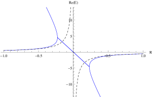
Figure 1: Real part of $E(R,t)$ for $t=0$ (dashed line) and $t=0.025$ (solid line), for $c_{\text{eff}}=1$

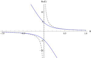
Figure 2: Real part of $E(R,t)$ for $t=0$ (dashed line) and $t=0.025$ (solid line), for $c_{\text{eff}}=-1$

As a last comment, one may wonder whether, for a generic model, the flow could produce more exotic types of singularities occurring at later times, not originating from the pole at $R=0$. However, while in general a solution of the hydrodynamic equation will undergo a sequence of wave-breaking events (depending on the number of bumps in its initial profile), we found no evidence that these should occur in the physical region $R>0$.

5 Identification of the perturbing operator

Let us now establish a direct link between the CDD-factor introduced in (10) and the $\text{T}\bar{\text{T}}$ operator. We start from equation (34):

$$\partial_{t}E_{n}(R,t)=E_{n}(R,t)\partial_{R}E_{n}(R,t)+{\textstyle\frac{1}{R}}P_{n}(R)^{2},$$ (42)

where $E_{n}(R,t)$ denotes the $n$-th excited state of the system on a ring of size $R$. It is convenient to consider the theory as defined on a cylinder or torus, with Euclidean coordinates $(x,y)\sim(x+R,y)$. The expectation values of the components of the stress-energy tensor on the eigenstates of the Hamiltonian defined on constant-$y$ slices, satisfy [5],

$$E_{n}(R,t)=-R\langle n|T_{yy}|n\rangle,\,\,\,\,\partial_{R}E_{n}(R,t)=-\langle n|T_{xx}|n\rangle,\,\,\,\,P_{n}=-iR\langle n|T_{xy}|n\rangle,$$ (43)

so that (42) can be rewritten as

$$\partial_{t}E_{n}(R,t) = R\left(\langle n|T_{yy}|n\rangle\langle n|T_{xx}|n\rangle-\langle n|T_{xy}|n\rangle\langle n|T_{xy}|n\rangle\right)$$ (44)

$$= -{\textstyle\frac{R}{\pi^{2}}}\left(\langle n|T|n\rangle\langle n|\bar{T}|n\rangle-\langle n|\Theta|n\rangle\langle n|\Theta|n\rangle\right).$$

In (44), we have used the standard conversion between the energy-momentum tensor components in Euclidean and complex coordinates,

$$T_{xx}=-{\textstyle\frac{1}{2\pi}}(\bar{T}+T-2\Theta)\,,\,\,T_{yy}={\textstyle\frac{1}{2\pi}}(\bar{T}+T+2\Theta)\,,\,\,\ T_{xy}={\textstyle\frac{i}{2\pi}}(\bar{T}-T).$$ (45)

One of the main results of [18] is the important identity

$$\langle n|\text{T}\bar{\text{T}}|n\rangle=\langle n|T|n\rangle\langle n|\bar{T}|n\rangle-\langle n|\Theta|n\rangle\langle n|\Theta|n\rangle,$$ (46)

which was established for a generic QFT in 2D and is based on a consistent, general definition, of the $\text{T}\bar{\text{T}}$ composite operator:

$$\text{T}\bar{\text{T}}(z,\bar{z}):=\lim_{(z,\bar{z})\rightarrow(z^{\prime},\bar{z}^{\prime})}T(z,\bar{z})\bar{T}(z^{\prime},\bar{z}^{\prime})-\Theta(z,\bar{z})\Theta(z^{\prime},\bar{z}^{\prime})+\text{total derivatives }.$$ (47)

Comparing (46) with the rhs of (44) leads to the identification:

$$\partial_{t}E_{n}(R,t)=-{\textstyle\frac{R}{\pi^{2}}}\langle n|\text{T}\bar{\text{T}}|n\rangle=-{\textstyle\frac{1}{\pi^{2}}}\langle n|\int_{0}^{R}dx\,\text{T}\bar{\text{T}}(z,\bar{z})|n\rangle.$$ (48)

After multiplying by $Le^{-LE_{n}(R,t)}$ and taking the trace, equation (48) can be rewritten as

$$\partial_{t}\ln Z(R,L,t)={\textstyle\frac{1}{\pi^{2}}}\langle\int_{0}^{R}dx\int_{0}^{L}dy\,\text{T}\bar{\text{T}}(z,\bar{z})\rangle,$$ (49)

where $Z(R,L,t)$ is the partition function of the perturbed system on a torus with characteristic lengths $(L,R)$. This suggests that, apart for total derivative terms, the Lagrangian density fulfils a simple local differential equation:

$$\partial_{t}{\mathcal{L}}(z,\bar{z},t)=-\frac{1}{\pi^{2}}\,\text{T}\bar{\text{T}}(z,\bar{z},t).$$ (50)

We conclude that

$${\mathcal{L}}(z,\bar{z},t)={\mathcal{L}}(z,\bar{z},0)-\frac{t}{\pi^{2}}\,\text{T}\bar{\text{T}}(z,\bar{z})+\mathcal{O}\left(t^{2}\right),$$ (51)

generalizing the CFT result of [9] to a massive quantum field theory. Equation (50) first appeared in [27] and is the main motivation for the analysis of the next Section.

6 From the free boson to Nambu-Goto

6.1 Single free boson

The aim of this Section is to show how the perturbed action can be computed recursively from equation (50), and to verify that, starting from the free-boson theory, the deformation generates the Nambu-Goto action for a string moving in $3D$ target space written in static gauge. We shall also present a closed formula for the infinite set of conserved currents, leading to local integrals of motion of this integrable theory. Our starting point is the free boson action :

$$A_{\text{CFT}}=\frac{1}{4}\int dx\,dy\,\left((\partial_{x}\phi)^{2}+(\partial_{y}\phi)^{2}\right)=\frac{1}{2}\int dz\,d\bar{z}\,\left(\partial_{z}\phi\,\partial_{\bar{z}}\phi\right)=\int dx\,dy\,\mathcal{L}_{\text{free}},$$ (52)

where $z=x+iy$, $\bar{z}=x-iy$, $\mathcal{L}_{\text{free}}=\partial\phi\,\bar{\partial}\phi$. For conciseness, let us introduce the rescaled energy-momentum components, $\tau=T/\pi$, $\bar{\tau}=\bar{T}/\pi$, $\theta=\bar{\theta}=\Theta/\pi$, and the composite operator $\tau\bar{\tau}=\text{T}\bar{\text{T}}/\pi^{2}$, so that the differential equation (50) will take the form

$$\partial_{t}{\mathcal{L}}(z,\bar{z},t)=-\tau\bar{\tau}(z,\bar{z},t).$$ (53)

We will use the canonical expression for the energy-momentum tensor in a generic Lagrangian theory with a single boson field, which yields

$$\tau=-\frac{\partial\mathcal{L}}{\partial\left(\bar{\partial}\phi\right)}\partial\phi,\quad\bar{\tau}=-\frac{\partial\mathcal{L}}{\partial\left(\partial\phi\right)}\bar{\partial}\phi,\quad\theta=\frac{1}{2}\,\left(\frac{\partial\mathcal{L}}{\partial\left(\partial\phi\right)}\partial\phi+\,\frac{\partial\mathcal{L}}{\partial\left(\bar{\partial}\phi\right)}\bar{\partial}\phi-2\mathcal{L}\right),$$ (54)

so that (53) takes the form of a simple partial differential equation for the Lagrangian density

$$\partial_{t}{\mathcal{L}}(z,\bar{z},t)=-\left(\frac{\partial\mathcal{L}}{\partial\left(\bar{\partial}\phi\right)}\partial\phi\right)\,\left(\frac{\partial\mathcal{L}}{\partial\left(\partial\phi\right)}\bar{\partial}\phi\right)+\frac{1}{4}\left(\frac{\partial\mathcal{L}}{\partial\left(\partial\phi\right)}\partial\phi+\,\frac{\partial\mathcal{L}}{\partial\left(\bar{\partial}\phi\right)}\bar{\partial}\phi-2\mathcal{L}\right)^{2},$$ (55)

where we are taking into account the definition of the composite field $\tau\bar{\tau}$ as

$$\tau\bar{\tau}(z,\bar{z})=\tau(z,\bar{z})\,\bar{\tau}(z,\bar{z})-\theta^{2}(z,\bar{z}).$$ (56)

In order to solve (53), we can setup a perturbative expansion in $t$,

$${\mathcal{L}}(z,\bar{z},t)=\sum_{j=0}^{\infty}t^{j}{\mathcal{L}}^{(j)}\;,$$ (57)

with initial condition ${\mathcal{L}}^{(0)}\equiv{\mathcal{L}}_{\text{free}}$, so that (55) translates into

$${\mathcal{L}}^{(j+1)}=-\frac{1}{j+1}\sum_{k=0}^{j}\left(\tau^{(k)}\;\bar{\tau}^{(j-k)}-\theta^{(k)}\;\theta^{(j-k)}\right),$$ (58)

with

$$\tau^{(j)}=-\frac{\partial{\mathcal{L}}^{(j)}}{\partial\left(\bar{\partial}\phi\right)}\partial\phi,\quad\bar{\tau}^{(j)}=-\frac{\partial{\mathcal{L}}^{(j)}}{\partial\left(\partial\phi\right)}\bar{\partial}\phi\;,\quad\theta^{(j)}=\frac{1}{2}\,\left(\frac{\partial{\mathcal{L}}^{(j)}}{\partial\left(\partial\phi\right)}\partial\phi+\,\frac{\partial{\mathcal{L}}^{(j)}}{\partial\left(\bar{\partial}\phi\right)}\bar{\partial}\phi-2{\mathcal{L}}^{(j)}\right)\;.$$

The first order is the familiar result for the energy-momentum tensor of the free boson:

$$\tau^{(0)}=\tau_{\text{free}}=-(\partial\phi)^{2}\;\;\;\;\;\;\bar{\tau}^{(0)}=\bar{\tau}_{\text{free}}=-(\bar{\partial}\phi)^{2},\;\;\;\;\;\theta^{(0)}=\theta_{\text{free}}=0.$$ (59)

Going through a few more orders, it is rather simple to find the form of the general solution

$${\mathcal{L}}^{(j)}=\binom{1/2}{j+1}\;2^{2j+1}\;\left({\mathcal{L}}^{(0)}\right)^{j+1}\;,$$ (60)

which can be verified by induction. Resumming the series, we find

$${\mathcal{L}}(z,\bar{z},t)=\frac{1}{2t}\left(-1+\sqrt{1+4t\,{\mathcal{L}}^{(0)}}\right)=-\frac{1}{2t}+\mathcal{L}_{\text{NG}}\;.$$ (61)

The Lagrangian density $\mathcal{L}_{\text{NG}}$ appearing above is the Nambu-Goto Lagrangian for a bosonic string in $D=3$ target space:

$$\mathcal{L}_{\text{NG}}\;dxdy=\frac{1}{2t}\,\sqrt{\text{det}(\sum_{\mu=1}^{D}\partial_{\alpha}X^{\mu}\,\partial_{\beta}X^{\mu})}\;dxdy,$$ (62)

with $D=3$, in the so-called static gauge:

$$X^{1}\rightarrow x\;\;\;\;X^{2}\rightarrow y,$$ (63)

where $x,\,y$ are Euclidean worldsheet coordinates, and where the transverse direction of oscillation $X^{3}$ is identified with the bosonic field, $X^{3}\rightarrow t^{\frac{1}{2}}\;\phi$.

Integrals of motion:

Let us conclude this Section by presenting the explicit form of the higher conserved currents of the model, $\left\{\tau_{n},\;\bar{\tau}_{n}\right\}_{n\in\mathbb{N}}$, satisfying the conservation equations:

$${\bar{\partial}}{\tau}_{n}={\partial}{\theta}_{n-2},\;\;\;\;\;\;{\partial}{\bar{\tau}}_{n}={\bar{\partial}}{\bar{\theta}}_{n-2},$$ (64)

which imply that the following quantities are local integrals of motion:

$$I_{n-1}=\oint\left(\tau_{n}(z,\bar{z})\,dz+{\theta}_{n-2}(z,\bar{z})\,d{\bar{z}}\right),\;\;\;\bar{I}_{n-1}=\oint\left(\bar{\tau}_{n}(z,\bar{z})\,d{\bar{z}}+{\bar{\theta}}_{n-2}(z,\bar{z})\,dz\right),$$ (65)

where $I_{1}+\bar{I}_{1}$ corresponds to the Hamiltonian of the theory. We obtained these currents as a deformation of following currents for the free theory at $t=0$:

$$\tau^{(0)}_{n}=-({\partial}\phi)^{n},\;\;\;\bar{\tau}^{(0)}_{n}=-({\bar{\partial}}\phi)^{n}.$$ (66)

The strategy of the construction is simply to enforce perturbatively at every order in $t$, the compatibility between the conservation equation (64) and the equations of motion descending from the variation of the Lagrangian (61),

$$\sum_{n=0}^{\infty}(-1)^{n}\left(\partial^{n}{\textstyle\frac{\partial{\cal L}}{\partial\partial^{n}\phi}}+\bar{\partial}^{n}{\textstyle\frac{\partial{\cal L}}{\partial\bar{\partial}^{n}\phi}}\right)=0,$$ (67)

which take the form

$$\partial\bar{\partial}\phi=t{\textstyle\frac{\bar{\partial}^{2}\phi(\partial\phi)^{2}+\partial^{2}\phi(\bar{\partial}\phi)^{2}}{1+2t\partial\phi\,{\bar{\partial}}\phi}}.$$ (68)

Omitting the details of the calculation, the exact form of the currents is the following:

$${\tau}_{n} = -\frac{({\partial}\phi)^{n}}{\sqrt{1+4t\;\mathcal{L}_{\text{free}}}}\,\left(\frac{2}{\sqrt{1+4t\;\mathcal{L}_{\text{free}}}+1}\right)^{n-2},$$ (69)

$${\theta}_{n-2} = -t\,\frac{({\partial}\phi)^{n}\,({\bar{\partial}}\phi)^{2}}{\sqrt{1+4t\;\mathcal{L}_{\text{free}}}}\;\left(\frac{2}{\sqrt{1+4t\;\mathcal{L}_{\text{free}}}+1}\right)^{n},$$ (70)

with a similar definition for $\bar{\tau}_{n}$ and $\bar{\theta}_{n-2}$. Notice that ${\tau}_{2}=\tau$ and ${\theta}_{0}=\theta$, where $\tau$ and $\theta$ are the components of the stress-energy tensor defined above, see (54).

Finally, it is noteworthy that the following rather surprising relation between the trace of the stress-energy tensor and the composite field $\tau\bar{\tau}$ holds at all orders in $t$:

$$\theta(z,\bar{z})=-t\,\tau\bar{\tau}(z,\bar{z}),$$ (71)

which implies

$$\tau\bar{\tau}(z,\bar{z})=\frac{1}{2t^{2}}\,\left(\sqrt{1+4t^{2}\tau(z,\bar{z})\,\bar{\tau}(z,\bar{z})}-1\right).$$ (72)

6.2 $N$ free bosons

Let us now consider the $t=0$ model as a theory of $N$ massless free bosons. It is simple to check directly that the Lagrangian:

$$\mathcal{L}=-\frac{1}{2t}+\mathcal{L}_{\textrm{NG}}^{N+2},\,\,\mathcal{L}_{\textrm{NG}}^{N+2}=\frac{1}{2t}\,\sqrt{1+4t\,\mathcal{L}_{\textrm{free}}^{N}-4t^{2}\mathcal{B}_{N}}\;,$$ (73)

with

$$\mathcal{L}_{\textrm{free}}^{N}=\sum_{i=1}^{N}\partial\phi_{i}\bar{\partial}\phi_{i}\;,\;\;\;\;\mathcal{B}_{N}=\;\sum_{i=1}^{N}\left(\partial\phi_{i}\right)^{2}\,\sum_{j=1}^{N}\left(\bar{\partial}\phi_{j}\right)^{2}-\left(\sum_{i=1}^{N}\partial\phi_{i}\bar{\partial}\phi_{i}\right)^{2}\;,$$ (74)

fulfils the appropriate generalization of (55) to a system of $N$ bosonic fields. The Lagrangian $\mathcal{L}_{\textrm{NG}}^{N+2}$ defined above can again be derived from the Nambu-Goto action (62), now in $D=N+2$ dimensions, imposing the static-gauge condition (63) and identifying the fields as transverse oscillation modes of the string: $X^{j+2}=t^{\frac{1}{2}}\;\phi_{j}$, $j=1,\dots,N$. One could also recover the same result from a perturbative construction similar to the one presented in the previous section. For completeness, we report the first few terms: setting $\mathcal{L}=\sum_{k=0}^{\infty}t^{k}\mathcal{L}^{(k)}$, we have

$$\mathcal{L}^{(0)} = \mathcal{L}_{\textrm{free}}^{N}\,,\,\,\mathcal{L}^{(1)}=-\left(\mathcal{L}_{\textrm{free}}^{N}\right)^{2}-\mathcal{B}_{N}\,,\,\,\mathcal{L}^{(2)}=2\left(\mathcal{L}_{\textrm{free}}^{N}\right)^{3}+2\mathcal{L}_{\textrm{free}}^{N}\,\mathcal{B}_{N}\;,$$

$$\mathcal{L}^{(3)} = -5\left(\mathcal{L}_{\textrm{free}}^{N}\right)^{4}-6\left(\mathcal{L}_{\textrm{free}}^{N}\right)^{2}\,\mathcal{B}_{N}-\mathcal{B}_{N}^{2}\,,\,\,\dots$$ (75)

Integrals of motion:

An infinite set of integrals of motion can also be constructed for the $N>1$ case. The equations of motion in this case generalize to:

$$\partial\bar{\partial}\phi_{i}=t\;\left({\bar{\partial}^{2}\phi_{i}\;\sum_{j=1}^{N}(\partial\phi_{j})^{2}+\partial^{2}\phi_{i}\;\sum_{j=1}^{N}(\bar{\partial}\phi_{j})^{2}}\right)/{\left(1+2t\;\sum_{j=1}^{N}\partial\phi_{j}{\bar{\partial}}\phi_{j}\right)}.$$ (76)

Using (76), we proved that the following currents are conserved:

$${\tau}_{n} = -\frac{(-\tau_{2}^{(0)})^{n/2}}{\sqrt{1+4t\;\mathcal{L}_{\textrm{free}}^{N}-4t^{2}\;\mathcal{B}_{N}}}\,\left(\frac{1}{2}+t\;\mathcal{L}_{\textrm{free}}^{N}+\sqrt{1+4t\;\mathcal{L}_{\textrm{free}}^{N}-4t^{2}\;\mathcal{B}_{N}}\right)^{1-n/2},$$ (77)

$${\theta}_{n-2} = t\,\frac{(-\tau_{2}^{(0)})^{n/2}\,{\bar{\tau}_{2}^{(0)}}}{\sqrt{1+4t\;\mathcal{L}_{\textrm{free}}^{N}-4\;t^{2}\;\mathcal{B}_{N}}}\;\left(\frac{1}{2}+t\;\mathcal{L}_{\textrm{free}}^{N}+\sqrt{1+4t\;\mathcal{L}_{\textrm{free}}^{N}-4t^{2}\;\mathcal{B}_{N}}\right)^{-n/2},$$ (78)

with

$$\tau_{2}^{(0)} = -\sum_{j=1}^{N}(\partial\phi_{j})^{2}\,,\,\,\bar{\tau}_{2}^{(0)}=-\sum_{j=1}^{N}(\bar{\partial}\phi_{j})^{2}.$$ (79)

Also in this case, there is a surprisingly simple relation between $\theta$ and $\tau\bar{\tau}$, given by (71).

6.3 Single bosonic field with generic potential

Finally we would like to consider another generalisation of the free boson, namely a system consisting of one boson interacting with an arbitrary potential $V(\phi)$:

$$\mathcal{L}^{V}=\,\partial\phi\bar{\partial}\phi+m^{2}V[\phi]\;.$$ (80)

Much in the same spirit as what we discussed for the free boson, we would like to follow the flow defined by the equation

$$\partial_{t}\mathcal{L}_{t}^{V}=-\tau\bar{\tau}\;,\qquad\mathcal{L}_{t=0}\equiv\mathcal{L}^{(0)}=\mathcal{L}^{V}.$$ (81)

Note that we are not requiring the potential $V[\phi]$ to give rise to an integrable theory. The only assumption we are making is that $V$ does not depend on the derivatives $\partial\phi$ and $\bar{\partial}\phi$. For $V[\phi]=\sin(\beta\phi)$, in particular, we recover the sine-Gordon model considered as our primary example in this paper – however integrability does not play any special role in the following analysis. The first few terms in the perturbative expansion $\mathcal{L}^{V}_{t}=\sum_{j=0}^{\infty}t^{j}{\mathcal{L}}^{(j)}\;$ are easily computed similarly to the previous sections:

$${\mathcal{L}}^{(1)} =-\mathcal{F}^{2}+\mathcal{V}^{2}\;,\qquad{\mathcal{L}}^{(2)}=2\mathcal{F}^{3}+\mathcal{F}^{2}\mathcal{V}+\mathcal{V}^{3}\;,\qquad{\mathcal{L}}^{(3)}=-5\mathcal{F}^{4}-4\mathcal{F}^{3}\mathcal{V}+\mathcal{V}^{4}\;,$$

$${\mathcal{L}}^{(4)} =14\mathcal{F}^{5}+15\mathcal{F}^{4}\mathcal{V}+2\mathcal{F}^{3}\mathcal{V}^{2}+\mathcal{V}^{5}\;,$$

where

$$\mathcal{F}=\partial\phi\bar{\partial}\phi\ \;,\qquad\mathcal{V}=m^{2}V[\phi]\;.$$ (83)

The general form of $\mathcal{L}^{(j)}$ is that of a polynomial in $\mathcal{F}$ and $\mathcal{V}$, whose coefficients are some combinatorial numbers. Although it is not immediately clear, it is easy to verify that the following closed form is valid:

$${\mathcal{L}}^{(j)} = \mathcal{V}^{j+1}+(-1)^{j}\,\sum_{k=0}^{\lfloor\frac{j+1}{2}\rfloor}\frac{4^{j-k}}{\sqrt{\pi}}\frac{\Gamma\left(j-k+\frac{1}{2}\right)}{({j-k+1})\Gamma\left(j-2k+1\right)}\,\frac{\mathcal{F}^{j-k+1}\mathcal{V}^{k}}{k!}\;$$ (84)

$$= \mathcal{V}^{j+1}+\frac{(-4)^{j}}{\sqrt{\pi}}\frac{\Gamma\left(j+\frac{1}{2}\right)}{\Gamma\left(j+2\right)}\;\mathcal{F}^{j+1}\;{}_{3}F_{2}\left(\left.\begin{array}[]{c c c c c}-1-j&,&\frac{1-j}{2}&,&-\frac{j}{2}\\ &\frac{1}{2}-j&,&-j\end{array}\,\right|-\frac{\mathcal{V}}{\mathcal{F}}\right)\;.$$ (87)

The final expression for the $t\neq 0$ Lagrangian is

$$\mathcal{L}_{t}^{V} =\frac{m^{2}V[\phi]}{1-tm^{2}V[\phi]}+\frac{1}{\sqrt{\pi}}\sum_{j=0}^{\infty}\left(-4t\right)^{j}\frac{\Gamma\left(j+\frac{1}{2}\right)}{\Gamma\left(j+2\right)}\,\left(\,\partial\phi\bar{\partial}\phi\right)^{j+1}$$

$$\;\;\times\,{}_{3}F_{2}\left(\left.\begin{array}[]{c c c c c}-1-j&,&\frac{1-j}{2}&,&-\frac{j}{2}\\ &\frac{1}{2}-j&,&-j\end{array}\,\right|-m^{2}\frac{V\left[\phi\right]}{\partial\phi\bar{\partial}\phi}\right)\;,$$ (90)

which we did not manage to simplify further. This expression reduces to the Nambu-Goto result (61) in the limit $m\rightarrow 0$, as can be checked using the fact that ${}_{3}F_{2}\rightarrow 1$ when its argument vanishes.

Finally, we remark that the CDD factor deformation of a free massive boson theory was considered in [20], where the first two orders of the perturbed action were constructed by a direct diagrammatic analysis, in perfect agreement with (90), which generalizes this result to all orders and to a generic potential.

7 Exact cylinder partition function

In this Section we consider the $t$-deformation of rational CFTs and show how to compute the modified cylinder partition function. This can be achieved, at least in principle, using exact formulas for the perturbed Affleck and Ludwig “ground-state degeneracy” (commonly known as g-function) [44, 45, 46, 47, 23, 48]. In the following, this method is applied to the theory of a free massless Majorana fermion: the Ising model CFT with conformal boundary conditions. The final analytic expression for the excited state g-functions is very simple, suggesting that the form of the result might be model independent. To support this conjecture, we will not work in the framework of the exact g-function formula extracted from [23], which would need to be generalized on a case-by-case basis. Instead, we shall adapt an alternative method originally devised by Lüscher and Weisz [22] for free massless bosons in the effective string theory context. This more general and powerful approach is implemented in Section 7.2, leading to a confirmation of the Ising model result, which appears to be valid for a generic CFT. The construction also provides a compact integral expression for the cylinder partition function in terms of the CFT data.

Let us start by setting the stage. The cylinder partition function of the theory, with boundary conditions $(\alpha,\beta)$ applied at the bottom and top of a cylinder of length $L$ and circumference $R$, can be written in two equivalent representations:

$$\mathcal{Z}_{(\alpha,\beta)}(L,R) =\sum_{n=0}^{\infty}e^{-RE^{(\alpha,\beta)}_{n}(L)}, \text{(open channel)},$$ (91)

$$=\sum_{n=0}^{\infty}g^{(\alpha)}_{n}(R)\,g^{(\beta)}_{n}(R)e^{-LE_{n}(R)}, \text{(closed channel)}.$$ (92)

The excited state g-function $g^{(\alpha)}_{n}(R)$ is defined by:

$$g^{(\alpha)}_{n}(R)=\langle\alpha|n\rangle,$$ (93)

where $|n\rangle$ are the, properly normalized, energy eigenvectors of the Hamiltonian defined on a ring with circumference $R$. For the $t$-deformed theory, the closed channel energies are given by (15), while the energies in the open channel take the generic form [9]:

$$E_{n}^{(\alpha,\beta)}(R,t;c_{\text{eff}})=-\frac{R}{2t}+\sqrt{\frac{R^{2}}{4t^{2}}+\frac{\pi}{t}\,\left(n-\frac{c_{\text{eff}}}{24}\right)},$$ (94)

where $c_{\text{eff}}$ depends on the conformal family of the state and the choice of boundary conditions translates into selection rules for the propagating states. In the following we will determine the form of the sub-leading coefficients $g_{n}^{(\alpha)}(R)$.

7.1 The Ising model CFT perturbed by $\text{T}\bar{\text{T}}$

We shall consider the theory of free massless Majorana fermions. Denoting with $p$ the momentum of the right mover and with $−q$ the momentum of the left mover, the two-body scattering amplitudes are

$$S_{\pm\pm}(p,q)=-1,\,\,S_{+-}(p,q)=S_{-+}(p,q)=S(p,q)=e^{-i2tp_{+}p_{-}}=e^{i2tpq},$$ (95)

where $p=p_{+}$ and $q=-p_{-}$ are the energies of right and left-moving pseudoparticles, respectively. The fundamental boundary reflection factor is [9]

$$\mathcal{R}_{0}(p)=e^{itp^{2}},$$ (96)

while the general boundary-perturbing reflection factor has the form

$$\mathcal{R}_{\vec{\delta}}(p)=\mathcal{R}_{0}(p)\prod_{j=1}^{\infty}\left(\mathcal{R}_{\delta_{j}}^{2j-1}(p)\right)\,,\,\,\,\,\mathcal{R}_{\delta_{j}}^{2j-1}(p)=e^{(ip)^{2j-1}\delta_{j}}.$$ (97)

Each factor in the product appearing in the rhs of (97) corresponds to a specific perturbation of the CFT boundary with a descendant of the identity operator, with coupling $\delta_{j}$. Let us first consider the ground state g-function. Following [23], this quantity can be computed as:

$$\ln\left(g^{(\alpha)}_{0}(R,t)\right)=\ln\langle\alpha|0\rangle^{\text{\tiny CFT}}+\ln\left({g_{0,\Sigma}}(R,t)\right)+\ln\left({g_{0}}(R,t)\right)+\ln\left({g_{\vec{\delta}}}(R,t)\right),\,\,$$ (98)

with $\alpha$ denoting one of the conformal boundary conditions $\alpha=(+),(-),(f)$ [23]. The four terms contributing to $g^{(\alpha)}_{0}(R,t)$ are in general:

$$\ln\langle(+)|0\rangle^{\text{\tiny CFT}}=\ln\langle(-)|0\rangle^{\text{\tiny CFT}}=-\ln\sqrt{2},\,\,\,\ \ln\langle(f)|0\rangle^{\text{\tiny CFT}}=0,$$ (99)

$$\ln({g_{0,\Sigma}}(R,t))=\sum_{j=1}^{\infty}\frac{1}{2j-1}\int_{\gamma_{0}}\frac{dp_{1}}{2\pi}...\int_{\gamma_{0}}\frac{dp_{2j-1}}{2\pi}\frac{\varphi(p_{1},p_{2})}{1+e^{\epsilon(p_{1})}}...\frac{\varphi(p_{2j-1},p_{1})}{1+e^{\epsilon(p_{2j-1})}},$$ (100)

$$\ln({g_{0}}(R,t))=\int_{\gamma_{0}}(\varphi_{0}(p)-\varphi(p,p)){\cal L}(p)\frac{dp}{2\pi},$$ (101)

$$\ln({g_{\delta}}(R,t))=\sum_{j}\ln{g_{\delta_{j}}}(R,t)=\sum_{j}\int_{\gamma_{0}}\varphi_{\delta_{j}}(p){\cal L}(p)\frac{dp}{2\pi},$$ (102)

where the integration contour is $\gamma_{0}={\mathbb{R}}^{+}$

$$\varphi(p,q) = -i\partial_{q}\ln{S(p,q)}=2tp\,,\,\,\,\varphi_{0}(p)=-i\partial_{p}\ln{\mathcal{R}_{0}(p)}=2tp,$$ (103)

$$\varphi_{\delta_{j}}(p) = -i\partial_{p}\ln{\mathcal{R}_{\delta_{j}}^{(2j-1)}(p)}=(-1)^{j-1}(2j-1)\delta_{j}p^{2j-2},$$ (104)

${\cal L}(p)=\ln{(1+e^{-\epsilon(p)})}$ and the pseudoenergy $\epsilon(p)$ solves the (periodic) TBA equation. From (103), we see that $\ln\left(g_{0}(R,t)\right)=0$, and

$$\begin{split}\ln\left({g_{0,\Sigma}}(R,t)\right)&=\sum_{j=1}^{\infty}\frac{1}{2j-1}\int_{\gamma_{0}}\frac{dp_{1}}{\pi}\frac{t\,p_{1}}{1+e^{\epsilon(p_{1})}}...\int_{\gamma_{0}}\frac{dp_{2j-1}}{\pi}\frac{t\,p_{2j-1}}{1+e^{\epsilon(p_{2j-1})}}\\ &=\sum_{j=1}^{\infty}\frac{1}{2j-1}\left(\int_{\gamma_{0}}\frac{dp}{\pi}\frac{t\,p}{1+e^{\epsilon(p)}}\right)^{2j-1}=\ln\sqrt{{\frac{1+A_{0}}{1-A_{0}}}},\end{split}$$ (105)

where

$$A_{0}=\int_{\gamma_{0}}\frac{dp}{\pi}\frac{t\,p}{1+e^{\epsilon(p)}}.$$ (106)

To find $A_{0}$, we recall that the relevant TBA equation is:

$$\epsilon(p)=Rp+pt\,E_{0}(R,t)\quad\Rightarrow\quad\partial_{p}\epsilon(p)=R+t\,E_{0}(R,t),$$ (107)

$$E_{0}(R,t)=-\int_{\gamma_{0}}\frac{dp}{\pi}{\cal L}(p)=-\int_{\gamma_{0}}\frac{dp}{2\pi}\frac{2p}{1+e^{\epsilon(p)}}\partial_{p}\epsilon(p).$$ (108)

Therefore,

$$E_{0}(R,t)=-\left(R+tE_{0}(R,t)\right)A_{0}/t\quad\Rightarrow\quad A_{0}=-\frac{t\,E_{0}(R,t)}{R+t\,E_{0}(R,t)}.$$ (109)

Considering that the boundary conditions impose that only zero-momentum states contribute to $\mathcal{Z}_{(\alpha,\beta)}(L,R)$, the generalization to excited states is obtained by replacing $\gamma_{0}={\mathbb{R}}^{+}$ with a contour $\gamma_{n}$ encircling zeros of $(1+e^{\varepsilon(p)})$ [49]. This means that $E_{0}\rightarrow E_{n}$ in (109). Going back to (105), the final result for the case $\vec{\delta}=0$ is

$$g_{n}^{(\alpha)}(R,t)=\langle\alpha|n\rangle^{\text{\tiny CFT}}\,\sqrt{\frac{R}{R+2t\,E_{n}(R,t)}}.$$ (110)

Equation (110) is the above mentioned simple formula for the deformed g-function. In the following section we shall prove that it remains valid for more general CFTs. One interesting aspect of the formula is that the “ground state degeneracy” $g_{0}$ diverges precisely at the critical value of the radius $R_{c}$ already discussed in Section 4.1. This is a further manifestation of the Hagedorn (tachyon) transition in the model.

Concerning the boundary corrections $(\ln{g_{\delta_{i}}})$, we find that the case $j=1$ is special:

$$\ln({g_{n,\delta_{1}}(R,t)})=\delta_{1}\int_{\gamma_{n}}\frac{dp}{2\pi}\,{\cal L}(p)=-\delta_{1}\frac{E_{n}(R,t)}{2},$$ (111)

as it amounts to a shift $L\rightarrow L+\delta_{1}$ (see also [9]):

$$\mathcal{Z}_{(\alpha,\beta)}(L,R,\delta_{1})=\mathcal{Z}_{(\alpha,\beta)}(L+\delta_{1},R,0).$$ (112)

The associated boundary correction to the action ${\cal A}$ is:

$$\delta{\cal A}_{\delta_{1}}={\textstyle\frac{\delta_{1}}{2}}\int_{0}^{R}dx\left(T_{yy}(x,0)+T_{yy}(x,L)\right).$$ (113)

For general values of $j$, we have

$$\ln\left({g_{\delta_{j}}}(R,t)\right) = (-1)^{j-1}\delta_{j}(2j-1)\int_{\gamma_{n}}\frac{dp}{2\pi}p^{2j-2}\ln{\left(1+e^{-(R+t\,E_{n}(R,t))p}\right)}$$ (114)

$$= (2j-1)(-1)^{j-1}\delta_{j}\left(R+t\,E_{n}(R,t)\right)^{1-2j}\int_{\gamma_{n}}\frac{dz}{2\pi}z^{2j-2}\ln{(1+e^{-z})}$$

$$= \frac{(-1)^{j}}{2\pi}\,\delta_{j}\left(R+t\,E_{n}(R,t)\right)^{1-2j}\,\Gamma(2j-1)\,{\text{Li}}^{(\gamma_{n})}_{2j}(-1).$$

In (114) a continuous branch of the polylogarithm, denoted as ${\text{Li}}^{(\gamma)}_{m}(z)$, is involved.

7.2 Cylinder partition function for more general perturbed CFT

To treat a more general case, let us recall that, on a cylinder geometry, the set of Virasoro characters $\chi_{i}$ (corresponding to a conformal module labelled by $i$) of a rational CFT fulfil the following duality property (see, [50]):

$$\chi_{i}(q) = q^{-c/24}\text{Tr}_{i}\left(q^{L_{0}}\right)\,,\,\,\,q=e^{-2\pi R/(2L)}\,,$$

$$\ \chi_{i}(q) = \sum_{j}S_{ij}\,\chi_{j}(\tilde{q})\,,\,\,\,\tilde{q}=e^{-4\pi L/R}.$$ (115)

This equation is directly related to the equivalence of the open/closed channel descriptions (91),(92) of the CFT partition function:

$$\begin{split}\mathcal{Z}^{\text{\tiny CFT}}_{\alpha\beta}(L,R)&=\text{Tr}(e^{-R\hat{H}_{(\alpha\beta)}(L)})=\sum_{i}n^{i}_{\alpha\beta}\chi_{i}(q)=\sum_{j}\langle\alpha|j\rangle^{\text{\tiny CFT}}\langle j|\beta\rangle^{\text{\tiny CFT}}\chi_{j}(\tilde{q})=\langle\alpha|e^{-L\hat{H}(R)}|\beta\rangle.\end{split}$$ (116)

Adapting an idea by Lüscher and Weisz [22], we can recover the $t$-deformed partition function as:

$$\mathcal{Z}_{\alpha\beta}(L,R) = \text{Tr}(e^{-R\hat{H}_{(\alpha\beta)}(L,t)})$$ (117)

$$= e^{-\frac{LR}{2t}}\,\sum_{i}n^{i}_{\alpha\beta}\int_{0}^{\infty}{\textstyle\frac{dv}{\sqrt{4\pi}v^{3/2}}}e^{-\left({\textstyle\frac{1}{4v}}+(\frac{LR}{2t})^{2}v\right)}\chi_{i}(e^{-\frac{\pi R^{2}v}{t}})$$

$$= e^{-\frac{LR}{2t}}\,\sum_{j}\langle\alpha|j\rangle^{\text{\tiny CFT}}\langle j|\beta\rangle^{\text{\tiny CFT}}\int_{0}^{\infty}{\textstyle\frac{dv}{\sqrt{4\pi}v^{3/2}}}e^{-\left({\textstyle\frac{1}{4v}}+(\frac{LR}{2t})^{2}v\right)}\chi_{j}(e^{-4t\pi/(R^{2}v)})$$

$$= \sum_{j,n}\langle\alpha|j\rangle^{\text{\tiny CFT}}\langle j|\beta\rangle^{\text{\tiny CFT}}\frac{R}{R+2t\,E_{(j,n)}(R,t)}e^{-LE_{(j,n)}(R,t)}$$

$$= \langle\alpha|e^{-L\hat{H}(R,t)}|\beta\rangle.$$

Therefore,

$$g_{\alpha,(j,n)}(R,t)=\langle\alpha|j\rangle^{\text{CFT}}\,\sqrt{\frac{R}{R+2t\,E_{(j,n)}(R,t)}}.$$ (118)

Equation (118) generalises the Ising model result (110) to arbitrary CFTs, correspondingly equations (117) provides a nice and compact integral representation for the perturbed partition function on a cylinder geometry.

8 Deformation of one-point correlation functions

The simple deformation rule (26) for the energy spectrum leads to similarly simple changes of other physical quantities, such as one-point correlation functions on a cylinder. In the following we shall implicitly assume that the $\text{T}\bar{\text{T}}$ perturbation deforms the spectrum of a generic 2D quantum field theory as

$$E_{n}(R,t)=E_{n}(R+t\,E_{n}(R,t),0)\,,$$ (119)

independently from the integrability property of the original model. Consider a set $\{\varphi_{i}\}$ of scalar fields and the corresponding perturbed action on a cylinder:

$${\cal A}_{(\vec{\bf g},0)}=\int_{cyl}\,dxdy\,{\cal L}_{(\vec{\bf g},0)}\,=\int_{cyl}\,dxdy\left({\cal L}_{\text{CFT}}+\sum_{i}\,g_{i}\varphi_{i}(x,y)\right).$$ (120)

One-point expectation values on this geometry can be obtained by differentiating the partition function $\mathcal{Z}(L,R,\vec{\bf g})$ as

$$\langle\varphi_{i}(0,0)\rangle_{R}=-\lim_{L\rightarrow\infty}\frac{1}{LR}\partial_{g_{i}}\ln\mathcal{Z}(L,R,\vec{\bf g})=\frac{1}{R}\partial_{g_{i}}E_{0}(R,\vec{\bf g}),\,\,\,$$ (121)

where $E_{0}(R,\vec{\bf g})$ is the ground state energy on the ring with circumference $R$. Without loss of generality, we can choose a normalization of the spectrum consistent with the TBA/NLIE framework, such that $E_{0}(R,\vec{\bf g})$ vanishes in the $R\rightarrow\infty$ limit. One-point expectation values on the plane are then encoded into the (anti) bulk coefficient ${\cal E}^{(\text{bulk})}(\vec{\bf g})$ in $E_{0}(R,\vec{\bf g})$ [5]:

$$E_{0}(R,\vec{\bf g})=E_{0}^{(\text{pert})}(R,\vec{\bf g})-{\cal E}^{(\text{bulk})}(\vec{\bf g},0)\,R,$$ (122)

where, at least in principle, the regular part $E_{0}^{(\text{pert})}(R,\vec{\bf g})$ can be obtained using CFT perturbation theory. Therefore

$$\langle\varphi_{i}(0,0)\rangle_{R}=\langle\varphi_{i}(0,0)\rangle_{R}^{(\text{pert})}-\langle\varphi_{i}(0,0)\rangle^{(\text{plane})}\,,\,\,\,\langle\varphi_{i}(0,0)\rangle^{(\text{plane})}=\partial_{g_{i}}{\cal E}^{(\text{bulk})}(\vec{\bf g},0)\,.$$ (123)

For integrable QFTs, a standard technique allows to identify ${\cal E}^{(\text{bulk})}(\vec{\bf g},0)$ by studying the $R\sim 0$ behaviour of TBA/NLIE equations [5, 51].

For the current discussion, it is not necessary to set the couplings $\left\{g_{i}\right\}$ in (121) to zero, so that the argument is valid also outside the (trivial) CFT limit, where all one-point functions would be zero on the cylinder. According to our assumptions, the $\text{T}\bar{\text{T}}$ deformation affects the ground state energy according to (119), and correspondingly one-point functions such as the ones defined in (121) are modified as

$$\langle\varphi_{i}(0,0)\rangle_{R}\rightarrow\langle\varphi_{i}^{(t)}(0,0)\rangle_{R,t} = \frac{1}{R}\,\frac{1}{(1-\left.t\,\partial_{R}E_{0}(R,\vec{\bf g})\right|_{R=\widetilde{R}})}\left.\partial_{g_{i}}E_{0}(R,\vec{\bf g})\right|_{R=\widetilde{R}}\,$$ (124)

$$= \frac{\widetilde{R}}{R}\frac{\langle\varphi_{i}(0,0)\rangle_{\widetilde{R},t=0}}{(1-\left.t\,\partial_{R}E_{0}(R,\vec{\bf g})\right|_{R=\widetilde{R}})},$$

where $\varphi_{i}^{(t)}(x,y)$ is a redefined field,

$$\varphi_{i}^{(t)}(x,y)=\partial_{g_{i}}{\cal L}_{(\vec{\bf g},t)}(x,y),$$ (125)

and $\widetilde{R}=R+t\,E_{0}(\widetilde{R},\vec{\bf g})$. Notice that in (124) the denominator vanishes precisely at the critical points discussed in Section 4.1. Apart from the universal factor in the denominator, the expectation values of the deformed fields $\varphi_{i}^{(t)}$ are simply connected by a change $R\rightarrow\tilde{R}$ to the undeformed ones in the $t=0$ theory. This replacement governs both the spectrum and one-point functions, and it is tempting to imagine that general correlation functions could also be obtainable by an equally simple rule. However, even for the deformed free boson case, there are many points in the previous derivation which cannot be straightforwardly adapted to the calculation of multi-point correlators. Finally, identifying the $\mathcal{O}(R)$ bulk coefficient ${\cal E}^{(\text{bulk})}(\vec{\bf g},t)$ from the small-$R$ behaviour of the ground state energy, we also find:

$$\langle\varphi_{i}^{(t)}(0,0)\rangle^{(\text{plane})}_{t}=\frac{\langle\varphi_{i}(0,0)\rangle^{(\text{plane})}_{t=0}}{(1+t\,{\cal E}^{(\text{bulk})}(\vec{\bf g},0))^{2}}.$$ (126)

The deformation of the fields, $\varphi_{i}\rightarrow\varphi_{i}^{(t)}$, appearing in (124) is a consequence of the nonlinearity of the definition of the $\text{T}\bar{\text{T}}$ operator, which generates, through (50), a nontrivial $\vec{\bf g}$-dependence in the Lagrangian ${\cal L}_{(\vec{\bf g},t)}$. It is interesting to look at the explicit expression for the deformed fields $\varphi_{i}^{(t)}$ for the models discussed in Section 6.

$\bullet$ Free massless bosons:

Let us start by considering the Lagrangian

$${\cal L}_{(g,0)}=\partial\phi\,\bar{\partial}\phi+g\,\varphi,$$ (127)

where $\varphi=f(\phi)$ is a generic field. We will apply the ideas of the previous section, setting $g\rightarrow 0$ at the end of the calculation to study the case of the pure $t$-deformation of a free massless boson. Therefore, we will compute $\left.\varphi^{(t)}=\partial_{g}{\cal L}_{(g,t)}\right|_{g=0}$. The deformed action ${\cal L}_{(g,t)}$ can be simply obtained from (90) with the replacement $m^{2}V(\phi)\rightarrow g\,\varphi$. We find

$$\partial_{g}\mathcal{L}_{(g,t)}\Big{|}_{g=0} = \varphi+\frac{\varphi}{2\sqrt{\pi}}\sum_{j=1}^{\infty}(-4t)^{j}\frac{\Gamma\left(j+\frac{1}{2}\right)}{\Gamma\left(j+2\right)}\left(\partial\phi\bar{\partial}\phi\right)^{j}\frac{j^{2}-1}{2j-1}$$

$$= \varphi-\frac{\varphi}{2}\left(1-\frac{1+2t\partial\phi\bar{\partial}\phi}{\sqrt{1+4t\partial\phi\bar{\partial}\phi}}\right).$$

Comparing with (69), the result above can be rewritten as

$$\partial_{g}\mathcal{L}_{(g,t)}\Big{|}_{g=0}=\varphi^{(t)}=\varphi\,[1-t\,\theta],$$ (128)

where the trace of the stress-energy tensor $\theta=\theta_{0}$ is defined in (69). While the formulae are more intricate, we checked that the final result (128) holds for the case of an arbitrary number of free bosons, with $\theta=\theta_{0}$ defined in (77).

$\bullet$ Single interacting boson:

In this case, the starting point is the Lagrangian for a single bosonic field with a generic potential:

$${\cal L}_{(g,m,0)}=\partial\phi\,\bar{\partial}\phi+m^{2}\,V(\phi)+g\,\varphi,$$ (129)

Setting ${\cal V}=m^{2}V(\phi)$, in this case we find

$$\varphi^{(t)} = \partial_{g}\mathcal{L}_{(g,m,t)}\Big{|}_{g=0}=\frac{\varphi}{\left(t{\cal V}-1\right)^{2}}$$

$$+ \frac{\varphi}{2\sqrt{\pi}}\sum_{j=1}^{\infty}(-4t)^{j}\frac{\Gamma\left(j+\frac{1}{2}\right)}{\Gamma\left(j+2\right)}\left(\partial\phi\bar{\partial}\phi\right)^{j}\frac{j^{2}-1}{2j-1}\;_{3}F_{2}\left(\left.\begin{array}[]{ccccc}-j&,&\frac{3-j}{2}&,&1-\frac{j}{2}\\ &\frac{3}{2}-j&,&1-j\end{array}\right|-\frac{{\cal V}}{\partial\phi\bar{\partial}\phi}\right)\;.$$

By a term by term inspection we found that the result can be rewritten in a very simple form:

$$\varphi^{(t)}=\varphi\,\left[1-2t\theta-t^{2}\left(\tau\bar{\tau}\right)\right]\;,$$ (131)

where the trace of the stress-energy tensor $\theta$ and the composite field $\tau\bar{\tau}$ are defined in the standard way in terms of the Lagrangian (129). Expression (8) reduces to the previous result (128) when ${\cal V}=0$, thanks to equation (71).

9 Conclusions

The study of 2D quantum field theories perturbed by irrelevant operators is still a largely unexplored research topic. These perturbations may lead to singular RG flows where the UV fixed point is not well-defined. An important arena where such flows appear prominently is the study of effective string theories, such as the ones used to describe confining flux tubes in non-Abelian gauge theories. Recently, some of the powerful tools associated to integrable models have made an appearance in this context, suggesting that exact results can be obtained for some of these irrelevant deformations. In this paper we investigated some general exact properties of a class of such flows related to the $\text{T}\bar{\text{T}}$ composite operator. Among the infinite number of possible perturbations of a given QFT, the latter operator displays very special and universal features.

From the point of view of a Lagrangian description, this deformation is formally defined through (50),(47). These equations were deduced using integrable models tools, such as the TBA and the NLIE, together with Zamolodchikov’s formula in [18], but can be considered as a definition of a special way of deforming an arbitrary QFT, irrespective of integrability. Moreover, under such a deformation, the energy levels evolve according to the simple hydrodynamic equation (34), where the deformation parameter $t$ enters as a formal time variable. This, in turn, allows to reconstruct the perturbed spectrum from the unperturbed energy levels through the simple non-linear mapping (33). For zero momentum states, in particular, (33) reduces to

$$E_{n}(R,t)=E_{n}(R+t\,E_{n}(R,t),0)\,.$$ (132)

Therefore, while the study of generic irrelevant perturbations in QFT by means of perturbative and non-perturbative methods remains very problematic, thanks to the exact mapping (33), (132), this perturbation appears to be surprisingly easy to treat. This fact may open the way to the study of conformal field theories perturbed by $\text{T}\bar{\text{T}}$ plus arbitrary, non necessarily integrable, combinations of relevant operators using the standard Truncated Conformal Space Approach (TCSA) [53] method or its RG-improved variant [54]. We feel that research on this topic may clarify important aspects concerning the appearance of singularities in effective QFT, and hopefully be useful in the effective string framework. It is well known that the flux tube spectrum is very well approximated, at relative large inter-quark separation, by the formula (15) or by its open-string analogous, but deviations are observed at intermediate length scales (see, for example [55] for a nice up-to-date compact review). Particularly interesting is the idea that also massive excitations could propagate on the flux-tube. It would be wonderful if TCSA could help to find a precise perturbed CFT interpretation of the pseudoscalar particle whose presence on the 4D QCD flux tube was recently conjectured on the basis of numerical data and TBA-inspired computations [7], or the massive mode discovered through Monte Carlo simulations in the 3D $U(1)$ gauge-theory [56].

It is important to stress that (15) was originally found by a light-cone-gauge quantization of the string, and that there is no known way to obtain this spectrum from a direct quantization of the static gauge action in a generic target space dimension $D\geq 3$. Furthermore, the light-cone spectrum is known to be incompatible with Lorentz invariance in the D-dimensional target space, except for the cases $D=3$ and $D=26$. In particular, a universal deviation from the spectrum (15) is observed at order $\mathcal{O}(1/R^{5})$ (for the excited states), when the string is quantized preserving target-space Lorentz invariance [57] (see also [58],[59],[55] for reviews). For this reason, we find remarkable that within the current setup, a direct correspondence between the spectrum (15) and the Nambu-Goto action written in static gauge is established in an arbitrary dimension. A possible explanation is suggested by the fact that perturbative calculations in [58] using the static-gauge action with a continuum, strictly two-dimensional regularization scheme show that the light-cone spectrum is reproduced at least up to – and including – order $\mathcal{O}(1/R^{5})$. The approach taken in this paper is indeed strictly two-dimensional, suggesting that, within the same class of schemes, the result is valid at all orders.

Coming back to the problem of target space Lorentz invariance, from the point of view of the current setup one may try to enforce this symmetry by adding further irrelevant operators, associated to corrections of the S-matrix, on top of the $\text{T}\bar{\text{T}}$-related ones considered in this paper. The form of the extra phase shift proposed in [61] for the $D=4$ case seems to suggest that the first additional perturbing operator is related to odd-spin symmetry generators, perhaps associated to some extended symmetry such as the $W_{3}$- algebra of the three states Potts model [62]. Despite obvious complications, it would be nice to study this issue and understand if the current approach can at least partially be modified to better approximate Lorentz-invariant effective string models.

Acknowledgments – We would like to thank Michele Caselle, Beatrice Conti, Davide Fioravanti, Ferdinando Gliozzi, Simone Piscaglia for useful discussions, and especially Sergei Dubovsky, Victor Gorbenko, Marco Meineri and Davide Vadacchino for clarifying discussions on issues related to effective string theories. We are also very grateful to Fedor Smirnov and Sasha Zamolodchikov for comments and encouragement at various points, and for sharing with us a copy of their paper “On space of integrable quantum field theories” [52] before publication.

The research leading to these results has received funding from the People Programme (Marie Curie Actions) of the European Union’s Seventh Framework Programme FP7/2007- 2013/ under REA Grant Agreement No 317089 (GATIS), and was partially supported by INFN grant FTECP and the UniTo-SanPaolo research grant Nr TO-Call3-2012-0088 “Modern Applications of String Theory” (MAST). The work of SN was supported by the European Research Council (Programme “Ideas” ERC- 2012-AdG 320769 AdS-CFT-solvable).

References

- [1] L. Onsager, Crystal statistics. i. a two-dimensional model with an order-disorder transition, Physical Review 65 (1944), no. 3-4 117.
- [2] R. Baxter, Exactly solved models in statistical mechanics. Courier Corporation, 2007.
- [3] F. H. Essler, H. Frahm, F. Göhmann, A. Klümper and V. E. Korepin, The one-dimensional Hubbard model. Cambridge University Press, 2005.
- [4] N. Beisert et. al., Review of AdS/CFT integrability: an overview, Lett. Math. Phys. 99 (2012) 3–32 [hep-th/1012.3982].
- [5] Al. B. Zamolodchikov, Thermodynamic Bethe ansatz in relativistic models. Scaling three state Potts and Lee-Yang models, Nucl. Phys. B 342 (1990) 695–720.
- [6] S. Dubovsky, R. Flauger and V. Gorbenko, Solving the simplest theory of quantum gravity, JHEP 2012 (2012), no. 9 1–36.
- [7] S. Dubovsky, R. Flauger and V. Gorbenko, Evidence from lattice data for a new particle on the worldsheet of the QCD flux tube, Phys. Rev. Lett. 111 (2013), no. 6 062006 [hep-th/1301.2325].
- [8] P. Goddard, J. Goldstone, C. Rebbi and C. B. Thorn, Quantum dynamics of a massless relativistic string, Nuclear Physics B 56 (1973), no. 1 109–135.
- [9] M. Caselle, D. Fioravanti, F. Gliozzi and R. Tateo, Quantisation of the effective string with TBA, JHEP 07 (2013) 071 [hep-th/1305.1278].
- [10] Al. B. Zamolodchikov, From tricritical ising to critical ising by thermodynamic bethe ansatz, Nuclear Physics B 358 (1991), no. 3 524–546.
- [11] Al. B. Zamolodchikov, Thermodynamics of imaginary coupled sine-gordon. dense polymer finite-size scaling function, Physics Letters B 335 (1994), no. 3-4 436–443.
- [12] T. R. Klassen and E. Melzer, Spectral flow between conformal field theories in 1+ 1 dimensions, Nuclear Physics B 370 (1992), no. 3 511–550.
- [13] P. Dorey, C. Dunning and R. Tateo, New families of flows between two-dimensional conformal field theories, Nuclear Physics B 578 (2000), no. 3 699–727.
- [14] C. Dunning, Massless flows between minimal W models, Physics Letters B 537 (2002), no. 3 297–305.
- [15] V. Fateev, D. Fradkin, S. L. Lukyanov, A. B Zamolodchikov, Al. B. Zamolodchikov, Expectation values of descendant fields in the sine-Gordon model, Nucl. Phys. B540 (1999) 587–609 [hep-th/9807236].
- [16] G. Delfino and G. Niccoli, The Composite operator T anti-T in sinh-Gordon and a series of massive minimal models, JHEP 05 (2006) 035 [hep-th/0602223].
- [17] G. Mussardo and P. Simon, Bosonic type S matrix, vacuum instability and CDD ambiguities, Nucl. Phys. B578 (2000) 527–551 [hep-th/9903072].
- [18] A. B. Zamolodchikov, Expectation value of composite field in two-dimensional quantum field theory, hep-th/0401146.
- [19] A. B. Zamolodchikov and Al.B. Zamolodchikov, Factorized S matrices in two-dimensions as the exact solutions of certain relativistic quantum field models, Annals Phys. 120 (1979) 253–291.
- [20] S. Dubovsky, V. Gorbenko and M. Mirbabayi, Natural tuning: towards a proof of concept, JHEP 09 (2013) 045 [hep-th/1305.6939].
- [21] P. Conkey and S. Dubovsky, Four loop scattering in the Nambu-Goto theory, JHEP 05 (2016) 071 [hep-th/1603.00719].
- [22] M. Lüscher and P. Weisz, String excitation energies in SU(N) gauge theories beyond the free-string approximation, JHEP 07 (2004) 014 [hep-th/0406205].
- [23] P. Dorey, C. Rim and R. Tateo, Exact g-function flow between conformal field theories, Nucl. Phys. B834 (2010) 485–501 [hep-th/0911.4969].
- [24] A. B. Zamolodchikov, “Effective field theories and integrability.” http://scgp.stonybrook.edu/video_portal/video.php?id=1669. Gauge Theory Program Seminar, SCGP, October, 2014.
- [25] F. Smirnov, “Form factors for relativistic and lattice models.” http://igst15.strongcoupling.org/node/7. Conference Talk at IGST15, KCL, March 2-6, 2015.
- [26] M. Lashkevich and Y. Pugai, Note on four-particle form factors of operators in sinh-Gordon model, J. Phys. A49 (2016), no. 30 305401 [hep-th/1602.05735].
- [27] A. B. Zamolodchikov, “Primus Inter Pares: Integrable Field Theories Among Common Ones.” http://scgp.stonybrook.edu/video_portal/video.php?id=1470. Workshop: ”Integrability vs. non-integrability in statistical mechanics”, SCGP, March 2-6, 2015.
- [28] F. Smirnov, Reductions of the sine-Gordon model as a perturbation of minimal models of conformal field theory, Nucl. Phys. B337 (1990) 156–180.
- [29] D. Bernard and A. Leclair, Residual quantum symmetries of the restricted sine-Gordon theories, Nucl. Phys. B340 (1990) 721–751.
- [30] A. Klümper, M. T. Batchelor and P. A. Pearce, Central charges of the 6- and 19-vertex models with twisted boundary conditions, Journal of Physics A: Mathematical and General 24 (1991), no. 13 3111–3133.
- [31] A. Klümper and P. Pearce, Conformal weights of RSOS lattice models and their fusion hierarchies, Physica A 183 (1992) 304.
- [32] P. Pearce and A. Klümper, Finite-size corrections and scaling dimensions of solvable lattice models: An analytic method, Phys. Rev. Lett. 66 (1991) 974–977.
- [33] C. Destri and H. de Vega, New thermodynamic Bethe ansatz equations without strings, Phys. Rev. Lett. 69 (Oct, 1992) 2313–2317.
- [34] C. Destri and H. De Vega, Unified approach to thermodynamic Bethe ansatz and finite size corrections for lattice models and field theories, Nuclear Physics B 438 (1995), no. 3 413–454.
- [35] V. V. Bazhanov, S. L. Lukyanov and A. B. Zamolodchikov, Integrable structure of conformal field theory, quantum KdV theory and thermodynamic Bethe ansatz, Commun. Math. Phys. 177 (1996) 381–398 [hep-th/9412229].
- [36] V. V. Bazhanov, S. L. Lukyanov and A. B. Zamolodchikov, Integrable structure of conformal field theory II. Q-operator and DDV equation, Communications in Mathematical Physics 190 (1997), no. 2 247–278.
- [37] V. V. Bazhanov, S. L. Lukyanov and A. B. Zamolodchikov, Integrable quantum field theories in finite volume: excited state energies, Nucl. Phys. B489 (1997) 487–531 [hep-th/9607099].
- [38] P. Dorey and R. Tateo, Excited states by analytic continuation of TBA equations, Nucl. Phys. B 482 (1996) 639–659 [hep-th/9607167].
- [39] D. Fioravanti, A. Mariottini, E. Quattrini and F. Ravanini, Excited state Destri-De Vega equation for sine-Gordon and restricted sine-Gordon models, Phys. Lett. B 390 (1997) 243–251 [hep-th/9608091].
- [40] G. Feverati, F. Ravanini and G. Takacs, Nonlinear integral equation and finite volume spectrum of sine-Gordon theory, Nucl. Phys. B540 (1999) 543–586 [hep-th/9805117].
- [41] Al. B. Zamolodchikov, Painleve III and 2-d polymers, Nucl. Phys. B432 (1994) 427–456 [hep-th/9409108].
- [42] G. B. Whitham, Linear and nonlinear waves, vol. 42. John Wiley and Sons, 2011.
- [43] D. Bessis and J. Fournier, Pole condensation and the Riemann surface associated with a shock in Burgers’ equation, Journal de Physique Lettres 45 (1984), no. 17 833–841.
- [44] I. Affleck and A. W. W. Ludwig, Universal noninteger ’ground state degeneracy’ in critical quantum systems, Phys. Rev. Lett. 67 (1991) 161–164.
- [45] A. LeClair, G. Mussardo, H. Saleur and S. Skorik, Boundary energy and boundary states in integrable quantum field theories, Nucl. Phys. B453 (1995) 581–618 [hep-th/9503227].
- [46] P. Dorey, I. Runkel, R. Tateo and G. Watts, g function flow in perturbed boundary conformal field theories, Nucl. Phys. B578 (2000) 85–122 [hep-th/9909216].
- [47] P. Dorey, D. Fioravanti, C. Rim and R. Tateo, Integrable quantum field theory with boundaries: the exact g function, Nucl. Phys. B696 (2004) 445–467 [hep-th/0404014].
- [48] B. Pozsgay, On O(1) contributions to the free energy in Bethe Ansatz systems: the exact g-function, JHEP 08 (2010) 090 [hep-th/1003.5542].
- [49] P. Dorey and R. Tateo, Excited states in some simple perturbed conformal field theories, Nucl. Phys. B 515 (1998) 575–623 [hep-th/9706140].
- [50] P. Di Francesco, P. Mathieu and D. Senechal, Conformal Field Theory. Graduate Texts in Contemporary Physics. Springer-Verlag, New York, 1997.
- [51] T. R. Klassen and E. Melzer, The thermodynamics of purely elastic scattering theories and conformal perturbation theory, Nucl. Phys. B 350 (1991), no. 3 635–689.
- [52] F. A. Smirnov and A. B. Zamolodchikov, On space of integrable quantum field theories, hep-th/1608.05499.
- [53] V. P. Yurov and A. B. Zamolodchikov, Truncated conformal space approach to scaling Lee-Yang model, Int. J. Mod. Phys. A5 (1990) 3221–3246.
- [54] P. Giokas and G. Watts, The renormalisation group for the truncated conformal space approach on the cylinder, hep-th/1106.2448.
- [55] B. B. Brandt and M. Meineri, Effective string description of confining flux tubes, hep-th/1603.06969.
- [56] M. Caselle, M. Panero, R. Pellegrini and D. Vadacchino, A different kind of string, JHEP 01 (2015) 105 [hep-lat/1406.5127].
- [57] O. Aharony and N. Klinghoffer, Corrections to Nambu-Goto energy levels from the effective string action, JHEP 12 (2010) 058 [hep-th/1008.2648].
- [58] O. Aharony and Z. Komargodski, The effective theory of long strings, JHEP 05 (2013) 118 [hep-th/1302.6257].
- [59] S. Dubovsky, R. Flauger and V. Gorbenko, Effective string theory revisited, JHEP 2012 (2012), no. 9 1–21.
- [60] S. Dubovsky and V. Gorbenko, Towards a theory of the QCD string, JHEP 02 (2016) 022 [hep-th/1511.01908].
- [61] S. Dubovsky, R. Flauger and V. Gorbenko, Flux tube spectra from approximate integrability at low energies, Journal of Experimental and Theoretical Physics 120 (2015), no. 3 399–422.
- [62] A. B. Zamolodchikov, Integrals of motion in scaling three state Potts model field theory, Int. J. Mod. Phys. A3 (1988) 743–750.