Mollow triplet: pump probe single photon spectroscopy of artificial atoms

Abstract

We analyze a photon transport through an 1D open waveguide side coupled to the $N$-photon microwave cavity with embedded artificial two- level atom (qubit). The qubit state is probed by a weak signal at the fundamental frequency of the waveguide. Within the formalism of projection operators and non-Hermitian Hamiltonian approach we develop a one-photon approximation scheme to obtain the photon wavefunction which allows for the calculation of the probability amplitudes of the spontaneous transitions between the levels of two Rabi doublets in $N$- photon cavity. We obtain analytic expressions for the transmission and reflection factors of the microwave signal through a waveguide, which contain the information of the qubit parameters. We show that for small number of cavity photons the Mollow spectrum consists of four spectral lines which is a direct manifestation of quantum nature of light. The results obtained in the paper are of general nature and can be applied to any type of qubits. The specific properties of the qubit are only encoded in the two parameters: the energy $\Omega$ of the qubit and its coupling $\lambda$ to the cavity photons.

I Introduction

The coherent coupling of a superconducting qubit to the microwave modes of a 1D coplanar waveguide transmission line has been intensely investigated over the last years both experimentally and theoretically. As compared with the conventional optical cavity with atomic gases, superconducting qubits as artificial atoms in solid-state devices have significant advantages, such as technological scalability, long coherence time which is important for the implementation of the quantum gate operations, huge tunability and controllability by external electromagnetic fields You11 ; Girvin09 ; Pashkin09 ; Sanders11 . Another advantage is an on-chip realization of strong and ultrastrong coupling regimes Wal04 ; Niemczyk10 previously inaccessible to atomic systems. This enables us to explore novel quantum phenomena emerging only in this regime. Furthermore, solid state superconducting circuits with embedded Josephson junction qubits have reproduced many physical phenomena known previously from quantum optics, such as Kerr nonlinearities Rebic09 ; Rehak14 , electromagnetically induced transparency Sun14 ; Abdumalikov10 ; Joo10 ; Li13 , the Mollow triplet Baur09 ; Astafiev10 ; Hoi12 ; Lang11 ; Toyli16 , and Autler-Townes splitting Sun14 ; Baur09 ; Sillanpaa09 .

As the Mollow triplet is a clear manifestation of the coherent nature of the light- matter interaction, its fluorescent or transmission spectra can be explained considering the pumping light classically Mollow69 . Instead of looking at the emission fluorescent spectrum we study here the transmission of a single photon which induces the transitions in a preliminary pumped cavity. The use of a single photon source as a probe reveals a marked influence of the quantum nature of light on the Mollow spectra and allows us to determine the response to the input of a single injected photon Lang11 ; Toyli16 ; Fink08 . Thus, a theoretical framework that allows one to directly calculate the response of such a system to a single injected photon is justified.

A conventional technique, which is used to study the photon transport in 1D geometry, is based on the master equation for the density matrix. It allows one to find analytic solution only for $N=1$ Om10 . For $N>1$ the solution of master equation are usually being solved approximately by numerical integration Bian09 . As to our knowledge, even for $N=2$ the analytic expressions for photon transport coefficients are not known.

From the other point, this technique is not quite suitable for single photon measurements since it operates with the average quantities. More appropriate approach for the description of a single photon transport is the calculation of the photon wavefunction which carries the information about quantum dynamics of the photon- matter interaction Shen05 ; Shen09 .

In the present paper we consider the transmission and reflection Mollow spectra for artificial atom (qubit) embedded in the $N$- photon cavity which is side- coupled to open microwave waveguide. We find the explicit expressions for the photon wavefunctions which describe the scattering of a single photon on the atom-cavity system with any value $N$ of preliminary pumped cavity photons.

Our analysis is based on the projection operators formalism and the method of the effective non- Hermitian Hamiltonian which has many applications for different open mesoscopic systems (see review paper Auerbach11 and references therein). Recently this method has been applied to photon transport through 1D open transmission line with $N$ embedded qubits Greenberg15 .

We find the analytic expressions for the probability amplitudes of the spontaneous transitions induced by injected photon in $N$- photon cavity. This enables us to find the forms of spectral lines depending on the qubit parameters and on the number of photons in a cavity. We show that for small number of cavity photons the transmission and reflection spectra consist of four lines which is a direct manifestation of quantum nature of light. As the number of cavity photons is increased two central peaks merge giving a conventional Mollow triplet.

The results obtained in the paper are relevant for the experiments where a qubit+cavity system is preliminary being driven by a fixed-frequency pump field to one of its excited $N$- photon states, with transitions to higher-lying states being studied by a weak, variable-frequency single photon probe Fink08 . Another application of our results is a phenomenon which is called a photon blockade. The excitation of the nonlinear atom-cavity system by a first photon at the frequency $\omega$ blocks the transmission of a second photon at the same frequency Birnbaum05 .

The paper is organized as follows. In Sec.II we briefly describe the projection operators formalism and the method of effective non hermitian Hamiltonian. In Sec.III we define the Hamiltonian of 1D waveguide side coupled to the $N$- photon microwave cavity with embedded qubit and qualitatively describe the process of a single photon scattering. The analytical expression for the effective non-hermitian Hamiltonian is given in Sec.IV. In this section we find the spectrum of the cavity resonances and their dependence on the cavity decay rate $\Gamma$, cavity-qubit coupling strength $\lambda$ and the number of cavity photons $N$. The wave function of the scattering photon is found in Sec.V, where we obtain the explicit analytical expressions for the probability amplitudes which describe spontaneous transitions between the levels of two Rabi doublets. These amplitudes are directly related to the transmission and reflection factors and show representative photon spectra. The results obtained in Sec.V are applied in Sec.VI where the transmission amplitudes have been analyzed in detail. In Sec.VI.1 we analyzed the case $N=2$ and showed that our results are consistent with the experiment in Fink08 . In addition, we show in Sec.VI.1 that in the experimental scheme of Fink et. al. Fink08 our results predicts the detection of a single photon with the frequency which is shifted from that of the input photon by a Rabi frequency. The probability amplitudes for this process are calculated. The application of our results to the description of photon blockade is given in Sec.VII.

II Projection formalism and effective non-hermitian Hamiltonian

We start with a brief review of projection formalism, highlighting only those aspects that will be required for the paper here. The application of this method to photon transport was described in more detail in Greenberg15 .

According to this method the Hilbert space of a quantum system with the Hermitian Hamiltonian $H$ is formally subdivided into two arbitrarily selected orthogonal projectors, $P$ and $Q$, which satisfy the following properties:

$$P+Q=1;\quad PQ=QP=0;\quad PP=P;\quad QQ=Q$$ (1)

Keeping in mind the scattering problem we assume that $Q$ subspace determines a closed system and, therefore, consists of discrete states, and $P$ subspace consists of the states from continuum. Those states of subspace Q which will turn out to be coupled to the states in subspace P will acquire the outgoing waves and become unstable. Then, for this scattering problem the effective Hamiltonian which describes the decay of Q- subsystem, becomes non Hermitian and has to be written as follows:

$${H_{eff}(E)}={H_{QQ}}+{H_{QP}}\frac{1}{{E-{H_{PP}+i\varepsilon}}}{H_{PQ}}$$ (2)

where $H_{XY}=XHY$, with $X,Y$ being $Q$ or $P$.

The effective Hamiltonian (2) determines the resonance energies of the Q- subsystem which are due to its interaction $H_{PQ}$ with continuum states from P- system. These resonances lie in the low half of the complex energy plane, $z=\rm{\widetilde{E}}-i\hbar\widetilde{\Gamma}$ and are given by the roots of the equation

$$D(z)\equiv\det\left({z-{H_{eff}}}\right)=0$$ (3)

The imaginary part $\widetilde{\Gamma}$ of the resonances describes the decay of $Q$- states due to their interaction with continuum $P$- states.

The scattering solution for the state vector of the Shrödinger equation $H\Psi=E\Psi$ reads Rotter01

$$|{\Psi}\rangle=\left|{in}\right\rangle+\frac{1}{{E-{H_{eff}}}}{H_{QP}}\left|{in}\right\rangle$$

$$+\frac{1}{{E-{H_{PP}}+i\varepsilon}}H_{PQ}\frac{1}{{E-{H_{eff}}}}{H_{QP}}\left|{in}\right\rangle\$$ (4)

where $|in\rangle$ is the initial state, which contains continuum variables and satisfies the equation $H_{PP}|in\rangle=E|in\rangle$.

The last term in the expression (II) describes to all orders of $H_{QP}$ the evolution of initial state $|in\rangle$ under the interaction between $P$ and $Q$ subspaces.

It is useful to stress that the formal results (2) and (II) do not require any explicit expressions for the projection operators.

III Single photon scattering

We consider a microwave 1D waveguide side coupled to a cavity with embedded qubit as is shown in Fig.1.

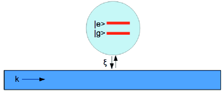
Figure 1: (Color online) Waveguide side coupled to the $N$- photon cavity with imbedded qubit

The Hamiltonian of the system reads:

$$H=\sum\limits_{k}{\hbar{\omega_{k}}c_{k}^{+}{c_{k}}}+\frac{1}{2}\hbar\Omega{\sigma_{z}}+\hbar{\omega_{c}}{a^{+}}a+\hbar\lambda(a^{+}+a){\sigma_{X}}$$

$$+\hbar\xi\sum\limits_{k}{(c_{k}^{+}a+{c_{k}}{a^{+}})}\quad\quad\quad\quad\quad\quad\quad\quad\quad\quad\quad\quad$$ (5)

where the first three terms are, respectively the Hamiltonian of waveguide photons, the Hamiltonian of the qubit with the excitation frequency $\Omega$, the Hamiltonian of one mode cavity. Fourth and fifth terms describe the qubit-cavity interaction with the strength $\lambda$, and the interaction between the waveguide and the cavity with the strength $\xi$.

As we study a single photon probe we assume that at every instant there is either one photon in a waveguide and $N-1$ photons in a cavity or no photons in a waveguide and $N$ photons in a cavity. Therefore, we assume that our Hilbert space is restricted to the following state vectors:

$$\left|1\right\rangle\equiv\left|0\right\rangle\otimes\left|{g,N}\right\rangle{\mkern 1.0mu},{\mkern 1.0mu}{\mkern 1.0mu}\left|2\right\rangle\equiv\left|0\right\rangle\otimes\left|{e,N-1}\right\rangle$$ (6)

$$\left|{{k_{1}}}\right\rangle\equiv\left|k\right\rangle\otimes\left|{g,N-1}\right\rangle{\mkern 1.0mu},{\mkern 1.0mu}{\mkern 1.0mu}\left|{{k_{2}}}\right\rangle\equiv\left|k\right\rangle\otimes\left|{e,N-2}\right\rangle$$ (7)

The states (6) correspond to no photons in a waveguide, $N$ photons in the cavity, and a qubit in the ground $g$ or excited state $e$. The states (7) correspond to the situation where one photon with a momentum $k$ is in a waveguide, $N-1$ photons in the cavity, and a qubit in the ground $g$ or excited state $e$.

Due to the interaction between cavity photons and a qubit each of the pair of states (6) and (7) are being hybridized to two pairs of dressed states $|\chi_{i,0}\rangle=|0\rangle\otimes|\chi_{i}\rangle$, $|\varphi_{i,k}\rangle=|k\rangle\otimes|\varphi_{i}\rangle$, where

$$|\chi_{i}\rangle=\alpha_{i}|g,N\rangle+\beta_{i}|e,N-1\rangle$$ (8)

$$|\varphi_{i}\rangle=a_{i}|g,N-1\rangle+b_{i}|e,N-2\rangle$$ (9)

Every pair of these dressed states are split by a Rabi frequency corresponding to the number of the cavity photons:

$$\Omega_{R}^{(N)}=\sqrt{{\Delta^{2}}+4{\lambda^{2}}N}$$ (10)

where $\Delta=\omega_{c}-\Omega$.

For subsequent calculations we need only the explicit form of the superposition factors $a_{i}$ and $b_{i}$ in (9) which can be expressed in terms of the angle variable $\theta$: $\tan 2\theta=-2\lambda(N-1)/\Delta$ with $a_{1}=b_{2}=\sin\theta$, $b_{1}=-a_{2}=\cos\theta$.

The process of the photon scattering can be qualitatively described as follows. Before a probing photon enters a waveguide the $N-1$ photon cavity + qubit system is in one of its hybridized states $|\varphi_{i}\rangle$($i=1,2$) (9) that was prepared by a preliminary pumping. The multiple interaction of a probing photon with a cavity leads to the formation of quasienergy hybridized states (8). These states subsequently decay with one photon being escaped to a waveguide, and a cavity + qubit system being left in one of the states (9). This picture is illustrated in Fig. 2 where the incoming photon excites the $|\varphi_{1}\rangle$ state to the state $|\chi_{2}\rangle$ at the frequency $\omega=\omega_{C}-\frac{1}{2}(\Omega_{R}^{(N)}+\Omega_{R}^{(N-1)})$. The state $|\chi_{2}\rangle$ subsequently decays either to the initial state $|\varphi_{1}\rangle$ with the outgoing photon having the excitation frequency $\omega$ or to the state $|\varphi_{2}\rangle$ with the outgoing photon having the frequency $\omega+\Omega_{R}^{(N-1)}$ .

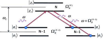
Figure 2: Color online. A scheme of a scattering of a single photon on the state $|\varphi_{1}\rangle$ of $(N-1)$- cavity when the transition $|\varphi_{1}\rangle\rightarrow|\chi_{2}\rangle$ is excited.

Hence there four possible outcomes of a probing photon scattering depending on which of the two states (9) were prepared by a preliminary pumping. These four possible channels are shown in Fig.3.

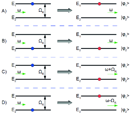
Figure 3: (Color online) Four outcomes of the scattering process. Two upper graphs correspond to elastic scattering, while two lower graphs correspond to inelastic sidebands. Blue circles denote the initial state, red ones denote the final state.

Two channels describe the elastic scattering when the initial and final states of the $N-1$ cavity + qubit system before and after scattering are the same, and the energies of incoming and outgoing photons are equal. The other two channels describe inelastic process when the outgoing photon gains or loses its energy by amount of $\hbar\Omega_{R}^{(N-1)}$. Every channel shown in Fig.3 corresponds to a specific transmission factor that will be calculated below. Each channel has two resonances which correspond to two transitions from $N$ photon cavity to one of the final states $\varphi_{i}$. For example, the channel $A$ in Fig.3 has one resonance at the frequency $\omega=\omega_{C}-\frac{1}{2}(\Omega_{R}^{(N)}+\Omega_{R}^{(N-1)})$ that induces the transition $|\varphi_{1}\rangle\rightarrow|\chi_{2}\rangle$ (see Fig.2). The other resonance is at the frequency $\omega=\omega_{C}+\frac{1}{2}(\Omega_{R}^{(N)}-\Omega_{R}^{(N-1)})$ that induces the transition $|\varphi_{1}\rangle\rightarrow|\chi_{1}\rangle$. Each of these resonances subsequently decays to the initial state $|\varphi_{1}\rangle$.

IV Cavity resonances

In accordance with the projection operators formalism we define two mutual orthogonal subspaces as follows

$$Q=|1\rangle\langle 1|+|2\rangle\langle 2|$$ (11)

$$P=\sum\limits_{k}{\sum\limits_{n=1}^{2}{\left|{{k_{n}}}\right\rangle\left\langle{{k_{n}}}\right|}}=\frac{L}{{2\pi}}\int{dk\sum\limits_{n=1}^{2}{\left|{{k_{n}}}\right\rangle\left\langle{{k_{n}}}\right|}}$$ (12)

where L is the length of waveguide, and the orthogonality condition for P subspace vectors is

$$\left\langle k_{n}\right.\left|{k^{\prime}_{m}}\right\rangle=\frac{{2\pi}}{L}\delta_{n,m}\delta\left({k_{n}-k^{\prime}_{m}}\right)$$ (13)

where $n,m=1,2$.

The application of the method requires the continuum state vectors to be the eigenfunctions of Hamiltonian $H_{PP}$. This is not the case for (7) since $H_{PP}$ couples two vectors $|k_{1}\rangle$ and $|k_{2}\rangle$. It is not difficult to show that the state vectors $\left|\varphi_{i,k}\right\rangle$ defined in (9), are the eigenfunctions of $H_{PP}$ with the energies

$${E_{i}}/\hbar=-\frac{1}{2}{\omega_{c}}+{\omega_{c}}(N-1)+{\omega}-\frac{1}{2}{\left({-1}\right)^{i}}{\Omega_{R}^{(N-1)}}$$ (14)

where $\omega$ is the frequency of incident photon.

The matrix elements of $H_{eff}$ in the $Q$ subspace is as follows

$$\left\langle{1|{H_{eff}}|1}\right\rangle={\omega_{C}}N-\frac{1}{2}\Omega-jN\Gamma$$ (15a)

$$\left\langle{2|{H_{eff}}|2}\right\rangle={\omega_{C}}(N-1)+\frac{1}{2}\Omega-j(N-1)\Gamma$$ (15b)

$$\left\langle{1|{H_{eff}}|2}\right\rangle=\left\langle{2|{H_{eff}}|1}\right\rangle=\lambda\sqrt{N}$$ (15c)

where we introduce the width of the cavity decay rate $\Gamma=L{\xi^{2}}/v_{g}$. The details of the calculation of Eqs. 15a, 15b, 15c are given in the Appendix B.

Due to the interaction of the $Q$ states (6) with continuum states (7) the former acquire the resonances whose energies and widths become dependent on the coupling parameter $\xi$ in Hamiltonian (III), which defines the width of the cavity decay rate $\Gamma$. These resonances are given by the complex roots of Eq.3. For $H_{eff}$ given by the matrix elements (15a), (15b), (15c) this equation reads:

$$D(z)=\left({z/\hbar+\frac{1}{2}\Omega-{\omega_{c}}N+jN\Gamma}\right)\\ \times\left({z/\hbar-\frac{1}{2}\Omega-{\omega_{c}}\left({N-1}\right)+j\left({N-1}\right)\Gamma}\right)-{\lambda^{2}}N=0$$ (16)

where the complex energy $z$ is given by (14) where the frequency of incident photon $\omega$ is replaced by the complex value $\widetilde{\omega}$.

Every of two $Q$ states (6) may decay in two ways: either to the state $|\varphi_{1,k}\rangle$ with the energy $E_{1}$ or to the state $|\varphi_{2,k}\rangle$ with the energy $E_{2}$.

Accordingly, in both cases $(i=1,2)$ we obtain:

$$D(E_{i})=(\omega-\widetilde{\omega}_{i+})(\omega-\widetilde{\omega}_{i-})$$ (17)

where $\omega_{i\pm}$ are complex roots of the equation (16).

$${\tilde{\omega}_{1,\pm}}={\omega_{C}}-\frac{1}{2}\left[{{\Omega_{R}^{(N-1)}}+j(2N-1)\Gamma}\right]$$

$$\pm\frac{1}{2}\sqrt{{{\left({\Delta-j\Gamma}\right)}^{2}}+4{\lambda^{2}}N}$$ (18a)

$${\tilde{\omega}_{2,\pm}}={\omega_{C}}+\frac{1}{2}\left[{{\Omega_{R}^{(N-1)}}-j(2N-1)\Gamma}\right]$$

$$\pm\frac{1}{2}\sqrt{{{\left({\Delta-j\Gamma}\right)}^{2}}+4{\lambda^{2}}N}$$ (18b)

Since ${\tilde{\omega}_{2,\pm}}={\tilde{\omega}_{1,\pm}}+\Omega_{R}^{(N-1)}$, the dependence of real and imaginary part of these resonances on $\Gamma$ is the same for both cases. The dependence of the resonance widths on $\Gamma$ is shown in Fig.4 for $\Delta=0$. The position of splitting corresponds to the point $2\lambda\sqrt{N}=\Gamma$.

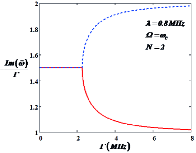
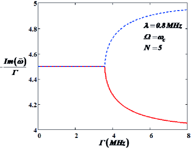
Figure 4: (Color online) The dependence of the resonance widths on the cavity decay rate $\Gamma$ for $\Delta=0$. For $\Gamma<2\lambda\sqrt{N}$ all widths are the same. The splitting starts at the point $\Gamma=2\lambda\sqrt{N}$. Dashed (blue) line corresponds to ${\tilde{\omega}_{1,-},\tilde{\omega}_{2,-}}$. Solid (red) line corresponds to ${\tilde{\omega}_{1,+},\tilde{\omega}_{2,+}}$

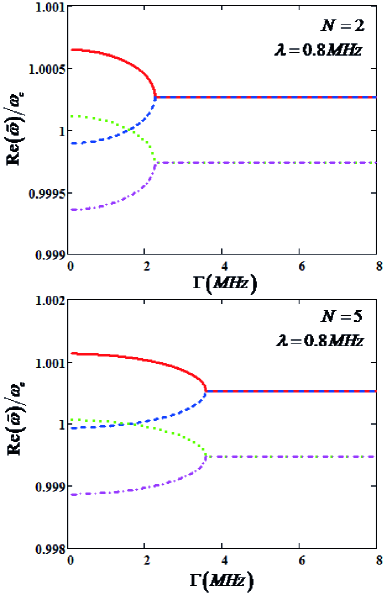
Figure 5: (Color online) The dependence of resonance energy on $\Gamma$ for $\Delta=0$. Upper curve corresponds to ${\tilde{\omega}_{2,\pm}}$, the lower one- to ${\tilde{\omega}_{1,\pm}}$. For $\Gamma>2\lambda\sqrt{N}$ the resonance energies do not depend on $\Gamma$ and shifted by $\Omega_{R}$. For $\Gamma<2\lambda\sqrt{N}$ there exist all four resonances separately.

The real parts of (18), (IV) correspond to the energy spacing between the levels of two manifolds shown in Fig.2. The transitions $\varphi_{1}\rightarrow\chi_{2}$, $\varphi_{1}\rightarrow\chi_{1}$, $\varphi_{2}\rightarrow\chi_{2}$, $\varphi_{2}\rightarrow\chi_{1}$ correspond to $Re(\widetilde{\omega}_{1-})$, $Re(\widetilde{\omega}_{1+})$, $Re(\widetilde{\omega}_{2-})$, $Re(\widetilde{\omega}_{2+})$, respectively.

Figure 5 shows the dependence of resonance energies on $\Gamma$ for $\Delta=0$, where for $\Gamma>2\lambda\sqrt{N}$ the resonance energies do not depend on $\Gamma$ and shifted by $\Omega_{R}^{(N-1)}$. For $\Gamma<2\lambda\sqrt{N}$ there exist all four resonances separately. For nonzero detuning $\Delta$ the widths are split for any $\Gamma$ as shown in the upper plot of Fig.6. The real parts of resonance energies displays all four components as shown in the lower plot of Fig.6. The dependence of resonances on the photon number $N$ for weak and strong coupling is shown in Fig.7 for zero frequency detuning $\Delta=0$. From (18), (IV) we can analyze the dependence of resonance frequencies on the coupling strength $\lambda$. For relatively small coupling $\lambda/\Gamma<1/2\sqrt{N}$, $Re(\widetilde{\omega}_{1+})=Re(\widetilde{\omega}_{1-})$ and $Re(\widetilde{\omega}_{1+})=Re(\widetilde{\omega}_{1-})$. The splitting begins at the point $\lambda/\Gamma=1/2\sqrt{N}$. As the ratio $\lambda/\Gamma$ is further increased, the frequencies (18), (IV) scale as follows: $Re(\widetilde{\omega}_{1-})\approx\omega_{c}-2\lambda\sqrt{N}$, $Re(\widetilde{\omega}_{2+})\approx\omega_{c}+2\lambda\sqrt{N}$, $Re(\widetilde{\omega}_{1+})\approx\omega_{c}+\lambda/2\sqrt{N},Re(\widetilde{\omega}_{2-})\approx\omega_{c}-\lambda/2\sqrt{N}$. These features are shown in Fig. 8 for zero detuning and $N=5$.

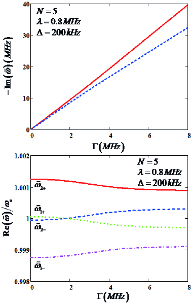
Figure 6: (Color online) The dependence of imaginary (upper plot) and real (lower plot) parts of resonances on $\Gamma$ for nonzero detuning. The solid (red) curve at upper plot corresponds to $\widetilde{\omega}_{1,2+}$, while the dashed (blue) curve corresponds to $\widetilde{\omega}_{1,2-}$

.

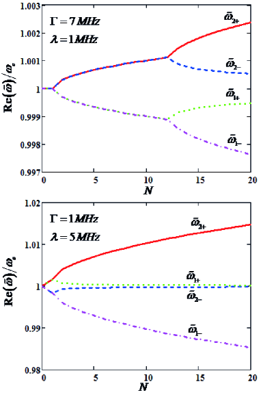
Figure 7: (Color online) The dependence of real parts of $\widetilde{\omega}_{1,\pm}$ and $\widetilde{\omega}_{2,\pm}$ for weak (upper plot) and strong (lower plot) coupling on the photon number $N$ for zero detuning.

.

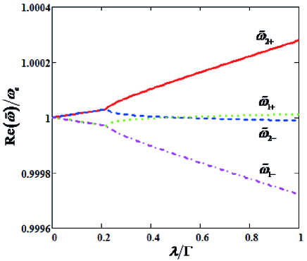
Figure 8: (Color online) The dependence of the positions of the resonance peaks on the coupling strength between qubit and cavity photons for $\Delta=0$ and $N=5$.

As we show in Sec.V, the transmission factors scales as $1/D(E_{1})$ or $1/D(E_{2})$. Therefore, the resonances of these quantities, which are given by the roots (18) and (IV) reflects the intrinsic properties of the cavity-qubit system. We will see below that transmission and reflection factors are peaked at the energies which correspond to the real parts of (18) and (IV).

V The wave function of the scattering photon

The key notion for the subsequent calculation of photon transmission and reflection is a transmission matrix

$$\left\langle{j,k^{\prime}}\right|T\left|{k,i}\right\rangle\\ =\sum\limits_{n,m=1}^{2}{\left\langle{{\varphi_{j,k^{\prime}}}}\right|{H_{PQ}}\left|n\right\rangle{R_{n,m}(E_{i})}\left\langle m\right|{H_{QP}}\left|{{\varphi_{i,k}}}\right\rangle}$$ (19)

where the matrix $R_{m,n}(E)=(\langle m|(E-H_{eff})|n\rangle)^{-1}$ is calculated in Appendix C.

In our case the transmission matrix (19) does not depend on the final momentum $k^{\prime}$ (detail are given in Appendix). The dependence of (19) on initial momentum $k$ is hidden in the energies $E_{i}$ (14), which depend on the frequency $\omega$ of incident photon.

The quantity (19) describes the process where the incident photon with momentum $k$ comes into interaction with a cavity that was initially in the state $|\varphi_{i}\rangle$ and then escapes with momentum $k^{\prime}$ leaving the cavity in the state $|\varphi_{j}\rangle$. Therefore, four different outcomes of this scattering processes for transmitted probe signal are possible: two of them correspond to elastic scattering and two of them correspond to inelastic process with the momenta of outgoing photon $k^{\prime}=k\pm\Omega_{R}^{(N-1)}/v_{g}$ (see Fig.3). According to these possibilities the initial state $|in\rangle$ in (II) corresponds to either $|\varphi_{1,k}\rangle$ or $|\varphi_{2,k}\rangle$.

$$|{\Psi_{1}}\rangle=\left|{{\varphi_{1,k}}}\right\rangle+\sum\limits_{m,n}{\left|n\right\rangle}{R_{nm}}({E_{1}})\left\langle m\right|{H_{QP}}\left|{{\varphi_{1,k}}}\right\rangle\\ +\sum\limits_{q,i}{\frac{{\left|{{\varphi_{i,q}}}\right\rangle}}{{{E_{1}}(k)-{E_{i}}(q)+i\varepsilon}}\left\langle{i,q}\right|T\left|{1,k}\right\rangle}$$ (20)

$$|{\Psi_{2}}\rangle=\left|{{\varphi_{2,k}}}\right\rangle+\sum\limits_{m,n}{\left|n\right\rangle}{R_{nm}}({E_{2}})\left\langle m\right|{H_{QP}}\left|{{\varphi_{2,k}}}\right\rangle\\ +\sum\limits_{q,i}{\frac{{\left|{{\varphi_{i,q}}}\right\rangle}}{{{E_{2}}(k)-{E_{i}}(q)+i\varepsilon}}\left\langle{i,q}\right|T\left|{2,k}\right\rangle}$$ (21)

From (20), (21) we obtain the photon wavefunctions in the configuration space $\langle x|\Psi_{1}\rangle$ and $\langle x|\Psi_{2}\rangle$:

$$\left\langle{x|{\Psi_{1}}}\right\rangle={e^{ikx}}\left|{{\varphi_{1}}}\right\rangle-i\Gamma{e^{ik\left|x\right|}}{t_{11}}\left|{{\varphi_{1}}}\right\rangle-i\Gamma{e^{i\left({k+k_{R}}\right)\left|x\right|}}{t_{21}}\left|{{\varphi_{2}}}\right\rangle$$ (22)

$$\left\langle{x|{\Psi_{2}}}\right\rangle={e^{ikx}}\left|{{\varphi_{2}}}\right\rangle-i\Gamma{e^{ik\left|x\right|}}{t_{22}}\left|{{\varphi_{2}}}\right\rangle-i\Gamma{e^{i\left({k-k_{R}}\right)\left|x\right|}}{t_{12}}\left|{{\varphi_{1}}}\right\rangle$$ (23)

where $k_{R}=\Omega_{R}^{(N-1)}/v_{g}$.

The quantities $t_{ij},i,j=1,2$ are the probability amplitudes for the spontaneous transitions between the levels of two Rabi doublets (see Fig.2). They are related to the transmission matrix as follows: $\left\langle{j,k^{\prime}}\right|T\left|{i,k}\right\rangle=\left\langle{{\varphi_{j}}}\right|T\left|{{\varphi_{i}}}\right\rangle\equiv\xi^{2}t_{j,i}$. The calculations, the details of which are given in the Appendix D, yield the following expressions for the probability amplitudes:

$$\begin{array}[]{l}t_{11}=\displaystyle\frac{1}{{4{\Omega_{R}^{(N-1)}}D({E_{1}})}}\\[14.22636pt] \quad\quad\quad\quad\times\left[{N({\Omega_{R}^{(N-1)}}+\Delta)\left({2\delta+\Delta+{\Omega_{R}^{(N-1)}}}\right)}\right.\\[8.5359pt] \quad\quad\quad\quad+(N-1)({\Omega_{R}^{(N-1)}}-\Delta)\left({2\delta-\Delta+{\Omega_{R}^{(N-1)}}}\right)\\[8.5359pt] \quad\quad\quad\quad+4jN(N-1){\Omega_{R}^{(N-1)}}\Gamma\left.{+8{\lambda^{2}}N(N-1)}\right]\end{array}$$ (24)

$$t_{21}=-\frac{{\lambda\sqrt{N-1}}}{{2{\Omega_{R}^{(N-1)}}D({E_{1}})}}\left({2\delta+{\Omega_{R}^{(N-1)}}-\Delta}\right)$$ (25)

$$\begin{array}[]{l}t_{22}=\displaystyle\frac{1}{{4{\Omega_{R}^{(N-1)}}D({E_{2}})}}\\[14.22636pt] \quad\quad\quad\quad\times\left[{N({\Omega_{R}^{(N-1)}}-\Delta)\left({2\delta+\Delta-{\Omega_{R}^{(N-1)}}}\right)}\right.\\[5.69046pt] \quad\quad\quad\quad+(N-1)({\Omega_{R}^{(N-1)}}+\Delta)\left({2\delta-{\Omega_{R}^{(N-1)}}-\Delta}\right)\\[5.69046pt] \quad\quad\quad\quad\left.{+4jN(N-1){\Omega_{R}^{(N-1)}}\Gamma-8{\lambda^{2}}N(N-1)}\right]\end{array}$$ (26)

$$t_{12}=-\frac{{\lambda\sqrt{N-1}}}{{2{\Omega_{R}^{(N-1)}}D({E_{2}})}}\left({2\delta-{\Omega_{R}^{(N-1)}}-\Delta}\right)$$ (27)

where $\delta=\omega-\omega_{c}$, $\Delta=\omega_{c}-\Omega$.

The positions of resonances are given by the points where the real parts of the complex roots of $D(E_{1})$ and $D(E_{2})$ are equal to zero. As it follows from (17) every quantity $t_{11},t_{21},t_{22},t_{12}$ has two resonant points, while the resonances of $t_{11}$ and $t_{21}$ (or for $t_{22}$ and $t_{12}$) lie at the same points. It is not difficult to find this resonance points for strong coupling ($\lambda\gg\Gamma$) and zero detuning ($\Delta=0$). The result is as follows:

$$\omega_{1}=\omega_{c}+\lambda(\sqrt{N}-\sqrt{N-1})$$ (28a)

$$\omega_{2}=\omega_{c}-\lambda(\sqrt{N}+\sqrt{N-1})$$ (28b)

for $t_{11}$ and $t_{21}$, and

$$\omega_{1}=\omega_{c}-\lambda(\sqrt{N}-\sqrt{N-1})$$ (29a)

$$\omega_{2}=\omega_{c}+\lambda(\sqrt{N}+\sqrt{N-1})$$ (29b)

for $t_{22}$ and $t_{12}$.

The equations (22) and (23) are the main results of our paper. They have a clear physical sense. The transmission signal (at $x>0$) consists of four waves: two elastic scattering waves with transmission factors $T_{11}=1-i\Gamma t_{11}$, $T_{22}=1-i\Gamma t_{22}$, and two inelastic scattering waves with transmission factors $T_{12}=-i\Gamma t_{12}$, $T_{21}=-i\Gamma t_{21}$. Accordingly, for reflection waves (at $x<0$) we have $R_{ij}=-i\Gamma t_{ij}$.

For every initial state the system was before the scattering there are two ways for incoming photon to be scattered (see Fig.3). This is seen in Eqs. (22) and (23) where the every scattering route is a superposition of two final states $|\varphi_{1}\rangle$ and $|\varphi_{2}\rangle$. The probability amplitudes $t_{11}$ (24), $t_{21}$ (25) correspond to the channels $A$ and $C$ in Fig.3, and the amplitudes $t_{22}$ (26), $t_{12}$ (27) correspond to the channels $B$ and $D$, respectively.

It is worth noting here that the probability amplitudes in (22), (23) describe different output photons. The amplitudes $t_{11}$ and $t_{22}$ are the probabilities to find the output photon with the same frequency as the frequency of the input photon, while the amplitudes $t_{21}$ and $t_{12}$ are the probabilities to find the output photon with the frequency which is shifted from the frequency of the input photon by a Rabi frequency $\Omega_{R}^{(N-1)}$.

We can show by the direct calculation that there exists an exact condition:

$$|T_{ii}|^{2}+|1-T_{ii}|^{2}+2|T_{ji}|^{2}=1$$ (30)

where $i,j=1,2$ and $i\neq j$ in third term in l.h.s. of (30). The left hand side of (30) is a sum of transmitted and reflected waves for every route shown in (22) and (23). It is tempting to consider the equation (30) as a condition of the energy flux conservation. However, in our case, as is seen from (22) and (23), the energies of the input and output photons may be different. The condition (30) reflects the conservation of probability: after the scattering the system must be definitely in one of the states, $|\varphi_{1}\rangle$ or $|\varphi_{2}\rangle$.

Since for every route (22) or (23) there are two outgoing photons with different frequencies we can measure separately all transmission $T_{ij}$ (or reflection $R_{ij}$) amplitudes.

VI Transmission spectra

As is well known the classical Mollow fluorescent spectrum consists of three lines. However, if the number of cavity photons is small the distance between the Rabi levels in neighbor Rabi doublets is not equal to each other: $\Omega_{R}^{(N)}>\Omega_{R}^{(N-1)}$. In this case the fluorescent spectrum for two adjacent doublets will consist of four spectral lines. These lines correspond to the spontaneous transitions between states (see Fig.2). $|\chi_{2}\rangle\rightarrow\varphi_{1}\rangle$, $|\chi_{2}\rangle\rightarrow\varphi_{2}\rangle$, $|\chi_{1}\rangle\rightarrow\varphi_{1}\rangle$, $|\chi_{1}\rangle\rightarrow\varphi_{2}\rangle$ with the corresponding frequencies of emitting photons: $\omega_{c}-\frac{1}{2}(\Omega_{R}^{N}+\Omega_{R}^{N-1})$, $\omega_{c}-\frac{1}{2}(\Omega_{R}^{N}-\Omega_{R}^{N-1})$, $\omega_{c}+\frac{1}{2}(\Omega_{R}^{N}-\Omega_{R}^{N-1})$, $\omega_{c}+\frac{1}{2}(\Omega_{R}^{N}+\Omega_{R}^{N-1})$.

The result of our study shows that we obtain the same frequencies for transmitted photons when studying the scattering of a single photon in 1D geometry via the system shown in Fig.1. In addition, we obtained the probability amplitudes (expressions (24), (25), (26), (27)) for spontaneous transitions between levels of two Rabi doublets (see Fig.2). Below we illustrate the application of our results to the transmission spectra for $N=2$ for strong resonance coupling when the distance between Rabi levels within $N$ manifold are given by $\Omega_{R}^{(N)}$ (10).

Having in mind to study the effects of adding to a cavity one extra photon we find the transmission and reflection factors for $N=1$ where we have either one photon in a waveguide and no photon in a cavity with a qubit being in its ground state or no photons in a waveguide and one photon in a cavity. In this case, as is seen from (24)-(26) the only quantity which is different from zero is $t_{11}$, so that for transmission and reflection we obtain:

$$T_{11}^{(N=1)}=\frac{{\left({\omega-{\omega_{+}}}\right)\left({\omega-{\omega_{-}}}\right)}}{{\left({\omega-{\omega_{+}}}\right)\left({\omega-{\omega_{-}}}\right)+j\Gamma\left({\omega-\Omega}\right)}}$$ (31)

$$R_{11}^{(N=1)}=\frac{{-j\Gamma\left({\omega-\Omega}\right)}}{{\left({\omega-{\omega_{+}}}\right)\left({\omega-{\omega_{-}}}\right)+j\Gamma\left({\omega-\Omega}\right)}}$$ (32)

where

$${\omega_{\pm}}=\frac{1}{2}\left({{\omega_{c}}+\Omega}\right)\pm\frac{1}{2}\Omega_{R}^{(1)}$$ (33)

The expressions (31) and (32) coincide with those known from the literature Shen09 . We have here two resonances at the frequencies $\omega_{\pm}$ with the distance between them being equal to Rabi frequency $\Omega_{R}^{(1)}$.

If we add one extra photon to the system we will also have two resonances for every route (22) or (23). But the picture is drastically different from the $N=1$ case. For example, if before scattering the system is in $|\varphi_{1}\rangle$ state, then each of the amplitudes $t_{11}$ and $t_{21}$ in (22) has two resonances at the same frequencies. The first resonance at $\omega_{c}-\frac{1}{2}(\Omega_{R}^{(2)}+\Omega_{R}^{(1)})$ corresponds to the transition from the state $|\varphi_{1}\rangle$ to the state $|\chi_{2}\rangle$ which subsequently decays either to the initial state $|\varphi_{1}\rangle$ (the probability of this process is given by the amplitude $t_{11}$ in (22)) or to the state $|\varphi_{2}\rangle$ with the probability being given by the amplitude $t_{21}$. The second resonance at $\omega_{c}+\frac{1}{2}(\Omega_{R}^{(2)}-\Omega_{R}^{(1)})$ corresponds to the transition from the state $|\varphi_{1}\rangle$ to the state $|\chi_{1}\rangle$ which subsequently decays either to the initial state $|\varphi_{1}\rangle$ with the probability $t_{11}$ or to the state $|\varphi_{2}\rangle$ with the probability $t_{21}$. Therefore, we see that each resonance corresponds to two outgoing photons: the frequency of the first photon is equal to the input frequency, the frequency of the second photon is increased as compared with the first one by the amount $\Omega_{R}^{(1)}$. Since the frequencies of these two photons are different, they can be detected separately and independently of each other.

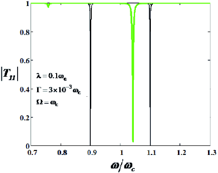
Figure 9: (Color online) Comparison of transmissions $T_{11}$ for $N=1$ (black, thin line) and $N=2$ (green, thick line) for strong resonant coupling.

In Fig.9 we compare the transmission coefficients $T_{11}$ for $N=1$ and $N=2$ as a function of the frequency of incident photon for the case of strong resonant coupling: $\lambda\gg\Gamma$, $\omega_{C}=\Omega$. Two dips which are symmetric relative to $\omega_{C}$ are calculated from expression (31). These dips are located at $\omega_{C}\pm\Omega_{R}^{(1)}$. The addition of one extra photon gives rise to the appearance of two dips, which results from the excitation of the level $|\varphi_{1}\rangle$. These dips are calculated from (24). A shallow dip, which is located at the frequency $\omega_{c}-\frac{1}{2}(\Omega_{R}^{(2)}+\Omega_{R}^{(1)})$ corresponds to the transition $|\varphi_{1}\rangle\rightarrow|\chi_{2}\rangle\rightarrow|\varphi_{1}\rangle$, while a deep dip, which is located at the frequency $\omega_{c}+\frac{1}{2}(\Omega_{R}^{(2)}-\Omega_{R}^{(1)})$ corresponds to the transition $|\varphi_{1}\rangle\rightarrow|\chi_{1}\rangle\rightarrow|\varphi_{1}\rangle$. The distance between two dips is equal to $\Omega_{R}^{(2)}$. For both cases the frequency of outgoing photons is equal to the frequency of the input photon.

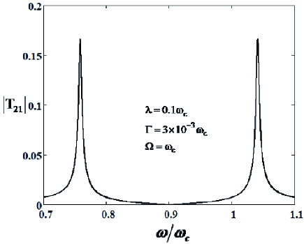
Figure 10: Inelastic transmission spectrum for $N=2$ and strong resonant coupling after the excitation of $|\varphi_{1}\rangle$ state. The outgoing photon leaves the cavity with the increased frequency $\omega+\Omega_{R}^{(1)}$.

In Fig.10 we show the transmission spectrum which is given by the amplitude $t_{21}$ in (22). Here the resonance points are the same as those in Fig.9, however, the outgoing photon has the increased frequency $\omega+\Omega_{R}^{(1)}$. After the scattering the cavity is being left in the state $|\varphi_{2}\rangle$. The left peak in Fig.10 corresponds to transitions $|\varphi_{1}\rangle\rightarrow|\chi_{2}\rangle\rightarrow|\varphi_{2}\rangle$ with the frequency of outgoing photon $\omega=\omega_{c}-\frac{1}{2}(\Omega_{R}^{(2)}-\Omega_{R}^{(1)})$. The right peak corresponds to transitions $|\varphi_{1}\rangle\rightarrow|\chi_{1}\rangle\rightarrow|\varphi_{2}\rangle$ with the frequency of outgoing photon $\omega=\omega_{c}+\frac{1}{2}(\Omega_{R}^{(2)}+\Omega_{R}^{(1)})$.

If initially the system is in the state $|\varphi_{2}\rangle$, the scattering wave function is given by (23). The resonance points are being shifted on the frequency axis to the right by $\Omega_{R}^{(1)}$. The first resonance at $\omega_{c}-\frac{1}{2}(\Omega_{R}^{(2)}-\Omega_{R}^{(1)})$ corresponds to the transition $|\varphi_{2}\rangle\rightarrow|\chi_{2}\rangle$ while the second one at $\omega_{c}+\frac{1}{2}(\Omega_{R}^{(2)}+\Omega_{R}^{(1)})$ corresponds to the transition $|\varphi_{2}\rangle\rightarrow|\chi_{1}\rangle$. Each of these excitations then decays either to the initial state $|\varphi_{2}\rangle$ with the probability amplitude $t_{22}$ or to the state $|\varphi_{1}\rangle$ with the probability amplitude $t_{12}$. The transmission spectrum for $N=2$ for the case when the system is left after scattering in the state $|\varphi_{2}\rangle$ is shown in Fig.11. This picture is similar to that shown in Fig.9. A deep dip, which is located at the frequency $\omega_{c}-\frac{1}{2}(\Omega_{R}^{(2)}-\Omega_{R}^{(1)})$ corresponds to the transition $|\varphi_{2}\rangle\rightarrow|\chi_{2}\rangle\rightarrow|\varphi_{2}\rangle$, while a shallow dip, which is located at the frequency $\omega_{c}+\frac{1}{2}(\Omega_{R}^{(2)}+\Omega_{R}^{(1)})$ corresponds to the transition $|\varphi_{2}\rangle\rightarrow|\chi_{1}\rangle\rightarrow|\varphi_{2}\rangle$. The distance between two dips is equal to $\Omega_{R}^{(2)}$. For both cases the frequency of outgoing photons is equal to the frequency of the input photon.

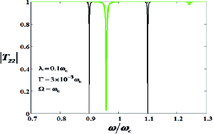
Figure 11: (Color online) Comparison of transmissions $T_{11}$ for $N=1$ (black, thin line) and $T_{22}$ for $N=2$ (green, thick line) for strong resonant coupling.

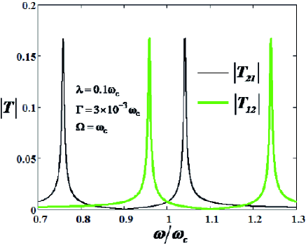
Figure 12: Color online. Inelastic transmission spectra for $N=2$ and strong resonant coupling after the excitation of the state $|\varphi_{1}\rangle$ (thin, black line) and the state $|\varphi_{2}\rangle$ (thick, green line).

In Fig.12 we show in one plot the transmission spectra which are given by the amplitudes $t_{21}$ in (22) and $t_{12}$ in (23). The black thin lines show the transmission spectrum when the system was initially in the state $|\varphi_{1}\rangle$ and after scattering was left in the state $|\varphi_{2}\rangle$ with the outgoing photon with the frequency increased by $\Omega_{R}^{(1)}$. These spectrum is the same as is shown in Fig.10. The green thick lines in Fig.12 show the transmission spectrum when the system was initially in the state $|\varphi_{2}\rangle$ and after scattering was left in the state $|\varphi_{1}\rangle$ with the outgoing photon with the frequency reduced by $\Omega_{R}^{(1)}$. The left peak of this spectrum corresponds to the excitation of the transition $|\varphi_{2}\rangle\rightarrow|\chi_{2}\rangle$ at the frequency of ingoing photon $\omega_{c}-\frac{1}{2}(\Omega_{R}^{(2)}-\Omega_{R}^{(1)})$. The state $|\chi_{2}\rangle$ then decays to the state $|\varphi_{1}\rangle$ with the frequency of outgoing photon $\omega_{c}-\frac{1}{2}(\Omega_{R}^{(2)}+\Omega_{R}^{(1)})$. The right peak corresponds to the excitation of the transition $|\varphi_{2}\rangle\rightarrow|\chi_{1}\rangle$ by the ingoing photon with the frequency $\omega_{c}+\frac{1}{2}(\Omega_{R}^{(2)}+\Omega_{R}^{(1)})$. The state $|\chi_{1}\rangle$ then decays to the state $|\varphi_{1}\rangle$ with the frequency of outgoing photon $\omega_{c}+\frac{1}{2}(\Omega_{R}^{(2)}-\Omega_{R}^{(1)})$.

VI.1 Comparison with the experiment

VI.1.1 The frequencies of the probing and detected photons are the same

We show here that our results shown in Fig.9 and Fig.11 correspond to those measured in Fink08 , where atom photon superposition states involving up to two photons have been studied, using a spectroscopic pump and probe technique. The experiments have been performed in a circuit QED setup, in which a superconducting qubit of transmon type has been embedded in a high-quality on-chip microwave cavity so that the frequency of the input (probing) photon and that of the output (detected) photon coincides. The level diagram of this system for $N=2$ is shown in Fig.13.

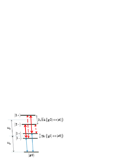
Figure 13: Color on line. Level diagram of a resonant cavity QED system for $N=2$ Fink08 . Thin blue arrows between $|g0\rangle$ and $|1\pm\rangle$ levels are responsible for the vacuum Rabi mode splitting which is shown by black dips in Fig.9 and Fig.11. Thick solid (red) arrows correspond to the green dips, and the solid dashed (red) lines correspond to shallow dips in Fig.9 and Fig.11.

The measurements were performed on resonance ($\omega_{c}=\Omega$) and under conditions of very strong coupling ($\lambda\gg\gamma$) where $\gamma$ is the qubit dephasing rate. The first and second Rabi doublets in Fig.13 are due to the hybridization of the bare qubit-photon states $|g1\rangle$, $|e0\rangle$, and $|g2\rangle$, $|e1\rangle$, respectively.

Our scheme is different from that of Ref.Fink08 in that we consider here a side coupled configuration with the open broad band waveguide while in Fink08 the measurements have been performed for direct coupled configuration with a high-$Q$ waveguide. However, the side coupled transmission coefficients $T_{11}$ and $T_{22}$ can be transformed to direct couple ones by a simple transformation Shen09 . The transmission spectra for direct coupling is equal to the side coupled reflection spectra: $T_{ii}^{dc}=1-T_{ii},(i=1,2)$. Hence, $T_{11}^{dc}=j\Gamma t_{11}$, $T_{22}^{dc}=j\Gamma t_{22}$, where $t_{11}$, $t_{22}$ are given in (24), (26), respectively. Therefore, the transmission spectra shown in Fig.4b and Fig.4d in Fink08 are the mirror reflection of the spectra shown in Fig.9 and Fig.11, respectively. Two dips in these figures which are symmetric relative to $\omega_{c}$ are the signature of vacuum Rabi mode splitting. For on resonant strong coupling these dips are located at $\omega=\omega_{c}\pm\lambda$ and correspond to the transitions between ground state $|g0\rangle$ and the states $|1+\rangle$ and $|1-\rangle$ (blue thin lines in Fig.13). For on resonance strong coupling conditions these dips give a full extinction of transmitted signal. However, if the bandwidth of the uncoupled waveguide is much smaller than the Rabi mode splitting the extinction can be very small (Fig.4b in Fink08 ).

The original idea in Fink08 was to measure the splitting of second Rabi doublet. By populating the levels $|1+\rangle$ or $|1-\rangle$ with a single photon they probed the transitions between $|1\pm\rangle$ and $|2\pm\rangle$ levels. The transitions $|1+\rangle\rightarrow|2+\rangle$, and $|1+\rangle\rightarrow|2-\rangle$, are described by the transmission amplitudes $T_{11}$, while the transitions $|1-\rangle\rightarrow|2-\rangle$ and, $|1-\rangle\rightarrow|2+\rangle$ are described by the transmission amplitudes $T_{22}$. The deep dips which are shown by green lines in Fig.9 and Fig.11 lie between vacuum Rabi modes lines. These dips which are located at the frequencies $\omega=\omega_{c}+(\sqrt{2}-1)\lambda$, $\omega=\omega_{c}-(\sqrt{2}-1)\lambda$ and correspond to the transitions $|1+\rangle\rightarrow|2+\rangle$ and $|1-\rangle\rightarrow|2-\rangle$ were observed in Fink08 (Fig.4b,d). However, they failed to observe the transitions $|1+\rangle\rightarrow|2-\rangle$ and $|1-\rangle\rightarrow|2+\rangle$ which are shown by dashed red lines in Fig.13. As was noted in Fink08 , the amplitudes of these transitions were very small to be observed. These amplitudes can be seen as shallow dips in Fig.9 and Fig.11. Using the data from Fink08 : $\omega_{c}/2\pi=6.94$ MHz, $\lambda/2\pi=154$ MHz, $\Gamma/2\pi=0.9$ MHz, we find from Eqs. 24, 26 the ratio of the amplitudes of the shallow dip to that of the main dip. For both cases shown in Fig.9 and Fig.11 this ratio is approximately equal to $3\times 10^{-3}$.

VI.1.2 The frequencies of the probing and detected photons are different

It is important that in Fink08 the frequencies of the input and output photons were the same. Thus, as we show above, the experimental results in Fink08 can be explained by the amplitudes $t_{11}$ and $t_{22}$ in Eqs. 22, 23.

However, the Eqs. 22, 23 predict another effect which at the best of our knowledge has not been observed in single photon experiments. We mean the registration of the output photon with a frequency shifted from that of the input photon by a Rabi frequency $\Omega_{R}^{(N-1)}$. The amplitudes responsible for this process are given by the quantities $t_{21}$ (25) and $t_{12}$ (27). The corresponding resonances are shown in Fig.12. The resonance frequencies in this figure correspond to the frequencies of the input photons which excite the transition in the cavity, but the frequency of the outgoing photons is different. For example, two peaks in Fig.10 correspond to the excitation of transitions (see Fig.13) $|1+\rangle\rightarrow|2-\rangle$ (left peak) and $|1+\rangle\rightarrow|2+\rangle$ (right peak) with subsequent decay to the state $|1-\rangle$ ($|2\pm\rangle\rightarrow|1-\rangle$) leaving the output photon with the frequency increased by $2\lambda$. Therefore, the amplitude of, for example, the left peak in Fig.10 should be interpreted as the probability to find the output photon with the frequency $\omega_{c}-(\sqrt{2}-1)\lambda$ if the frequency of the input photon is $\omega_{c}-(\sqrt{2}+1)\lambda$.

The detection of the output photons with the frequency different from that of the input photons can be realized using a vector network analyzer at the output of a broadband (low $Q$) waveguide. In order to detune from the input photons it is better to measure the reflected spectra. For broadband waveguide the reflected coefficient is given by the quantity

$${|R_{i}|}\equiv\left|{\left\langle{x|{\Psi_{i}}}\right\rangle-{e^{ikx}}\left|{{\varphi_{i}}}\right\rangle}\right|=\Gamma\sqrt{{{\left|{{t_{ii}}}\right|}^{2}}+{{\left|{{t_{ji}}}\right|}^{2}}}$$ (34)

where $i,j=1,2$ and $i\neq j$ in $t_{ji}$ in r.h.s of (14). The quantities $R_{1}$ and $R_{2}$ correspond to the preliminary populated levels $|1+\rangle$ and $|1-\rangle$, respectively.

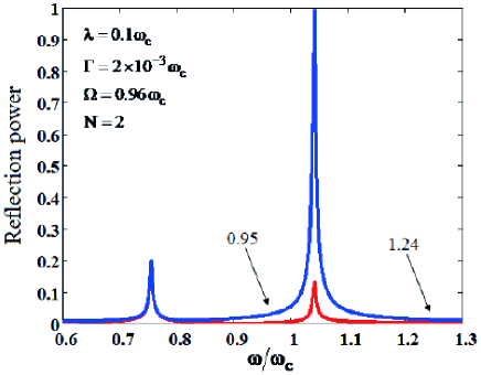
Figure 14: Reflection spectrum for broadband single photon detection. Black arrows show the frequency of the output photon the frequency of which is greater than the frequency of the input photon by the value of Rabi splitting $\Omega_{R}^{(1)}$. See text for details.

The reflection spectrum for the case when the level $|1+\rangle$ is preliminary populated is shown in Fig.14 by a thick blue line. The left peak at the point $\omega/\omega_{c}\approx 0.75$ is formed mainly by the contribution of $t_{21}$. As we explained before, this peak gives the probability to find the output photon at the frequency increased by $2\lambda$. This point is shown by the left arrow in Fig.14. A central large blue peak is formed mainly by the contribution of $t_{11}$. It means that at this input frequency $\omega\approx 1.04\omega_{c}$ we observe the output photon with the same frequency. However, a small contribution of $t_{21}$ to the central peak (shown by thin red line peak at $\omega/\omega_{c}\approx 1.04$) results in the output photon at the frequency $\omega\approx 1.24\omega_{c}$ (shown by the right arrow in Fig.14.

The same picture exists for the case when the level $|1-\rangle$ is preliminary populated. Here the reflection is given by the quantity $R_{2}$, and the output photons with the frequency decreased by $2\lambda$ can be observed.

VII A signature of the photon blockade in the transmission spectra

A concept of the photon blockade, in which transmission of only one photon through a system is possible while excess photons are absorbed or reflected, was first proposed in Imam97 . Since then there have been published the plethora of papers devoted to this phenomenon in different atom-cavity systems (see, for example, recent papers Deng17 ; Baj13 and references there in). The photon blockade is observed when the atom- photon interaction results in the energy spectrum with a nonlinear dependence on the number of cavity photons $n$. It can be either Kerr- type $n^{2}$ nonlinearity when the resonance frequency is largely detuned from the qubit energy (so called, a dispersive photon blockade Hoffman11 ) or the resonant photon blockade with Jaynes- Cummings $\sqrt{n}$ dependence Birnbaum05 . The photon blockade are usually investigated using the correlation function measurements of the photon statistics at the cavity output Birnbaum05 ; Lang11 . Alternatively, the signature of the photon blockade can be found as staircase pattern in the dependence of transmitted power on the incident photon bandwidth Hoffman11 .

Below we show the signature of the photon blockade in the transmission of a single photons one-by-one through a waveguide side coupled to the resonance cavity with a two-level atom (see Fig.1). In our scheme the photon blockade manifests as the transmission of a photon at some frequency $\omega$ if the preceding photon with the same frequency $\omega$ have been captured by the cavity. Or, alternatively, it may be observed at the input: if the input photon at some frequency $\omega$ is captured by the cavity, we, first, observe the reflected signal, and, second, the following photon with the same frequency passes through waveguide producing no reflected signal.

Even if initially there is no photons in a cavity, the first input photon with the frequency $\omega=\Omega$ is blocked to enter the cavity, it is completely transmitted as it follows from Eq.31. It can be captured by the cavity with simultaneous appearance of reflected signal only if its frequency is equal to $\omega_{\pm}$ (see Eq.32). The adding of a second photon with the frequencies $\omega_{\pm}$ cannot excite the cavity since there are no appropriate energy levels in the cavity with two photons with the energies $2\hbar\omega_{\pm}$ as it is shown in Fig.15. There is a frequency gap within which a second photon cannot be captured by a cavity.

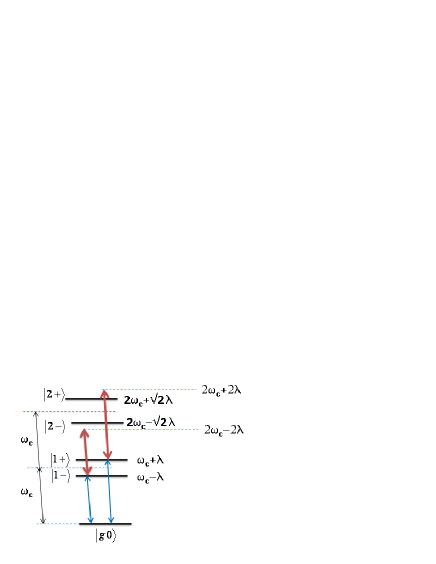
Figure 15: Color online. The level structure for on resonance strong coupling limit. Photon blockade manifests as the suppression of two- photon absorption for a probe field of frequency $\omega_{p}=\omega_{c}-\lambda$ or $\omega_{p}=\omega_{c}+\lambda$ (thick red arrows) tuned to excite the transition $|g0\rangle\rightarrow|1-\rangle$ or $|g0\rangle\rightarrow|1+\rangle$. The frequency gap in both cases is equal to $(2-\sqrt{2})\lambda$.

Below we show that in our scheme the photon blockade appears as the staircase pattern in the dependence of the reflected power on the detector bandwidth $\Delta\omega$ centered at $\omega_{c}$. First, we excite the cavity by a single photon with the energy corresponding to one of the hybridized level ($|N_{p}-\rangle$ or $|N_{p}+\rangle$) . This level successively undergoes one- photon decays to lower hybridized states. Every of these transitions produces a reflected signal at the corresponding frequency. Hence, under repeated excitation of the levels $|N_{p}\pm\rangle$ we obtain a reflected power as a discrete number of peaks, which number depends on $N_{p}$.

Figure 16: Reflected power spectral function $W_{N}(\omega)$ for $N=1$ (solid lines), $N=2$ (dotted line), and $N=3$ (dashed lines). The calculations is made for $\omega_{c}=\Omega=3$ GHz, $\lambda=0.1\omega_{c},\Gamma=2.66\times 10^{-3}\omega_{c}$. $\Delta\omega$ is a variable bandwidth of the detector .

Therefore, we define the reflected power in the detector bandwidth $\Delta\omega$ as follows:

$${P_{R}}({N_{p}},\Delta\omega)=\sum\limits_{N=1}^{{N_{p}}}{\int\limits_{{\omega_{c}}-\Delta\omega}^{{\omega_{c}}+\Delta\omega}{{{\left|{W_{N}(\omega)}\right|}^{2}}d\omega}}$$ (35)

where a spectral function $W_{N}(\omega)=|R_{1}+R_{2}|^{2}$ for $N>1$ with $R_{1},R_{2}$ being defined in (34), and $W_{1}(\omega)=R_{11}^{(N=1)}$, where $R_{11}^{(N=1)}$ is defined in (32). For $N>1$ the quantity $W_{N}(\omega)$ corresponds to the transitions $|N,\pm\rangle\rightarrow|N-1,\pm\rangle$, while $W_{1}(\omega)$ describes the transitions to the ground state $|1,\pm\rangle\rightarrow|g,0\rangle$.

The example of reflected power spectrum for first three $N^{\prime}$s is shown in Fig.16. It is seen that as $N$ is increased the width of resonance lines is also increased, which is understandable from the inspections of expressions (18) and (IV).

The application of the prescription encoded in (35) to the spectrum shown in Fig.14, provides a typical photon blockade ladder depicted in Fig.17. A higher doublet ladder includes all steps from the lower doublets. The height of a step scales as the width of the corresponding resonance. The slope of a step is increased as the emission rate $\Gamma$ of the photons from the cavity is also increased.

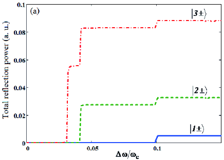
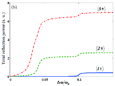
Figure 17: Photon blockade staircase. The calculations are made for $\omega_{c}=\Omega=3$ GHz, $\lambda=0.1\omega_{c}$, (a) $\Gamma=3.33\times 10^{-5}\omega_{c}=0.1MHz$, and (b) $\Gamma=2.66\times 10^{-3}\omega_{c}=8MHz$. $|N\pm\rangle$ denotes the preliminary pumped doublet which successively through one photon emissions decays to the ground state $|g0\rangle$. The steps from $|1\pm\rangle$ and $|2\pm\rangle$ doublet ladders are seen in the $|3\pm\rangle$ doublet ladder. Both plots were normalized to $10$ MHz.

VIII Conclusion

We develop a theoretical method for the calculation of a microwave transport in 1D waveguide side coupled to a resonant $N$-photon cavity with embedded artificial atom (qubit). The method is based on the projection operator formalism and a non-Hermitian Hamiltonian approach, which enables us to obtain the analytical expressions for the probability amplitudes of spontaneous transitions between the dressed levels of adjacent doublets in $N$- photon cavity. We show that if the number of the cavity photons is small the transmitted and reflected spectra reveal a quadruplet structure with two central peaks and two sidebands. As the number of the cavity photons is increased the two central peaks merge giving a classical Mollow triplet.

We considered in detail a single photon transport for the cavity with two photons. We showed that our theory is in accordance with the known experiment Fink08 . Moreover, it predicts the detection in a single photon experiment of the output photon which frequency is shifted from that of the input photon by a Rabi frequency $\Omega_{R}^{(N-1)}$. We also discussed in detail the applications of our results to the detection of the photon blockade ladder which is a direct manifestation of the quantum nature of light which results from a different space between the levels in adjacent Rabi doublets.

The results obtained in the paper can be applied to the investigation of microwave photon transport in superconducting circuits with embedded superconducting qubits based on Josephson junctionsYou11 ; Wal04 . The specific properties of the qubit are encoded in only two parameters: the qubit energy $\Omega$ and its coupling to the cavity $\lambda$. For example, for a superconducting qubit $\,\Omega=\sqrt{\varepsilon^{2}+\Delta^{2}}$ where $\varepsilon=\frac{2I_{q}}{\hbar}\left(\Phi_{x}-\Phi_{0}/2\right)$ is an external parameter which by virtue of external magnetic flux, $\Phi_{X}$ controls the gap between ground and excited states Wal00 , $I_{q}$ is a persistent current along a qubit loop, $\Phi_{0}=h/2e$ is a flux quantum. The quantity $\Delta$ is the qubit’s gap at the degeneracy point ($\varepsilon=0$). The coupling strength $\lambda=g\Delta/\Omega$ Om10 , where $g$ is the qubit-cavity coupling at the degeneracy point. For a charge qubit $\,\Omega=\sqrt{\varepsilon^{2}_{J}+\varepsilon^{2}_{C}}$ where $\varepsilon_{J}=2E_{J}|cos(\pi\Phi_{x}/\Phi_{0}|$, $\varepsilon_{C}=4E_{C}(1-2n_{g})$, where $E_{J}$ is a coupling energy of Josephson junction, $E_{C}$ is a charging energy, $n_{g}$ is a dimensionless gate charge which can be tuned by applying the voltage $V_{g}$ to the gate capacitance $C_{g}$: $n_{g}=C_{g}V_{g}/e$ Blais04 .

In a more general sense our results can be applied to the investigation of the photon transport in 1D qubit systems with small number of cavity photons.

Appendix A The calculation of $H_{XY}$

With the aid of explicit expressions (11) and (12) for $Q$ and $P$ we obtain for the parts $H_{XY}$ of the full Hamiltonian (III) the following expressions:

$${H_{QQ}}=\frac{1}{2}\hbar\Omega\left|2\right\rangle\left\langle 2\right|-\frac{1}{2}\hbar\Omega\left|1\right\rangle\left\langle 1\right|+\hbar{\omega_{c}}\left({N-1}\right)\left|2\right\rangle\left\langle 2\right|\\ +\hbar\lambda\sqrt{N}\left|1\right\rangle\left\langle 2\right|+\hbar\lambda\sqrt{N}\left|2\right\rangle\left\langle 1\right|+\hbar{\omega_{c}}N\left|1\right\rangle\left\langle 1\right|$$ (36)

$${H_{PP}}=\frac{1}{2}\hbar\Omega\sum\limits_{k}{\left|{{k_{2}}}\right\rangle\left\langle{{k_{2}}}\right|}+\hbar{\omega_{c}}\left({N-1}\right)\sum\limits_{k}{\left|{{k_{1}}}\right\rangle\left\langle{{k_{1}}}\right|}\\ +\hbar\lambda\sqrt{N-1}\sum\limits_{k}{\left|{{k_{1}}}\right\rangle\left\langle{{k_{2}}}\right|}+\hbar\lambda\sqrt{N-1}\sum\limits_{k}{\left|{{k_{2}}}\right\rangle\left\langle{{k_{1}}}\right|}\\ +\sum\limits_{k}{\hbar{\omega_{k}}\left|{{k_{1}}}\right\rangle\left\langle{{k_{1}}}\right|}+\sum\limits_{k}{\hbar{\omega_{k}}\left|{{k_{2}}}\right\rangle\left\langle{{k_{2}}}\right|}\\ +\hbar{\omega_{c}}\left({N-2}\right)\sum\limits_{k}{\left|{{k_{2}}}\right\rangle\left\langle{{k_{2}}}\right|}-\frac{1}{2}\hbar\Omega\sum\limits_{k}{\left|{{k_{1}}}\right\rangle\left\langle{{k_{1}}}\right|}$$ (37)

$${H_{PQ}}=\hbar\xi\sqrt{N-1}\sum\limits_{k}{\left|{{k_{2}}}\right\rangle\left\langle 2\right|}+\hbar\xi\sqrt{N}\sum\limits_{k}{\left|{{k_{1}}}\right\rangle\left\langle 1\right|}$$ (38)

$${H_{QP}}=\hbar\xi\sqrt{N}\sum\limits_{k}{\left|1\right\rangle\left\langle{{k_{1}}}\right|}+\hbar\xi\sqrt{N-1}\sum\limits_{k}{\left|2\right\rangle\left\langle{{k_{2}}}\right|}$$ (39)

Appendix B Calculation of the effective Hamiltonian

From (2) we find the matrix elements of effective hamiltonian in $Q$ subspace.

$$\begin{array}[]{l}\left\langle m\right|{H_{eff}}\left|n\right\rangle=\left\langle m\right|{H_{QQ}}\left|n\right\rangle\\ +\sum\limits_{\scriptstyle i,j=1\hfill\atop\scriptstyle k,k^{\prime}\hfill}^{2}{\left\langle m\right|{H_{QP}}\left|{{\varphi_{i,k}}}\right\rangle\left\langle{{\varphi_{i,k}}}\right|\frac{1}{{E-{H_{PP}}+i\varepsilon}}\left|{{\varphi_{j,k^{\prime}}}}\right\rangle\left\langle{{\varphi_{j,k^{\prime}}}}\right|{H_{PQ}}\left|n\right\rangle}\\ =\left\langle m\right|{H_{QQ}}\left|n\right\rangle+\sum\limits_{i=1,k}^{i=2}\displaystyle{\frac{{\left\langle m\right|{H_{QP}}\left|{{\varphi_{i,k}}}\right\rangle\left\langle{{\varphi_{{\mathop{\rm i}\nolimits},k}}}\right|{H_{PQ}}\left|n\right\rangle}}{{E-{E_{i}}(k)+i\varepsilon}}}\end{array}$$ (40)

Fortunately, the matrix elements $\left\langle m\right|{H_{QP}}\left|{{\varphi_{i,k}}}\right\rangle$ and $\left\langle{{\varphi_{i,k}}}\right|{H_{PQ}}\left|n\right\rangle$ do not depend on the photon momentum $k$. The direct calculations yield:

$$\left\langle{1|{H_{QP}}|{\varphi_{1,k}}}\right\rangle={a_{1}}\xi\sqrt{N},\quad\left\langle{2|{H_{QP}}|{\varphi_{1,k}}}\right\rangle={b_{1}}\xi\sqrt{N-1}$$ (41)

$$\left\langle{1|{H_{QP}}|{\varphi_{2,k}}}\right\rangle={a_{2}}\xi\sqrt{N},\quad\left\langle{2|{H_{QP}}|{\varphi_{2,k}}}\right\rangle={b_{2}}\xi\sqrt{N-1}$$ (42)

With the use of (36) and (41), (42) we obtain for the matrix elements of (40):

$$\left\langle{1|{H_{eff}}|1}\right\rangle={\omega_{C}}N-\frac{1}{2}\Omega+a_{1}^{2}{\xi^{2}}N{J_{1}}(E)+a_{2}^{2}{\xi^{2}}N{J_{2}}(E)$$ (43a)

$$\left\langle{2|{H_{eff}}|2}\right\rangle={\omega_{C}}(N-1)+\frac{1}{2}\Omega+b_{1}^{2}{\xi^{2}}(N-1){J_{1}}(E)\\ +b_{2}^{2}{\xi^{2}}(N-1){J_{2}}(E)$$ (43b)

$$\left\langle{1|{H_{eff}}|2}\right\rangle=\left\langle{2|{H_{eff}}|1}\right\rangle=\lambda\sqrt{N}\\[5.69046pt] +a_{1}{b_{1}}{\xi^{2}}\sqrt{N(N-1)}{J_{1}}(E)+a_{2}{b_{2}}{\xi^{2}}\sqrt{N(N-1)}{J_{2}}(E)$$ (43c)

where

$${J_{j}}(E)=\sum\limits_{k}{\frac{1}{{E-{E_{j}}(k)+i\varepsilon}}}=\frac{L}{{2\pi}}\int{\frac{{dk}}{{E-{E_{j}}(k)+i\varepsilon}}}$$ (44)

It will be shown below that all quantities $J_{j}(E)$ in (43a), (43b), and (43c) are the same and do not depend on the running energy $E$.

$${J_{j}}(E)=-\frac{{2\pi i}}{{{{\rm{v}}_{g}}}}$$ (45)

where $v_{g}$ is the velocity of microwave photons in a waveguide.

Finally, with the use of properties of coefficients $a_{i},b_{i}$ from in (9): $a_{1}^{2}+a_{2}^{2}=1$, $b_{1}^{2}+b_{2}^{2}=1$, $a_{1}b_{1}+a_{2}b_{2}=0$ we obtain for the matrix elements of $H_{eff}$ the following expressions:

$$\left\langle{1|{H_{eff}}|1}\right\rangle={\omega_{C}}N-\frac{1}{2}\Omega-jN\Gamma$$ (46a)

$$\left\langle{2|{H_{eff}}|2}\right\rangle={\omega_{C}}(N-1)+\frac{1}{2}\Omega-j(N-1)\Gamma$$ (46b)

$$\left\langle{1|{H_{eff}}|2}\right\rangle=\left\langle{2|{H_{eff}}|1}\right\rangle=\lambda\sqrt{N}$$ (46c)

where we introduce the width of the cavity decay rate $\Gamma=L{\xi^{2}}/v_{g}$.

Appendix C Calculation of the matrix R

Here we calculate the natrix $R_{m,n}(E)$ which is the matrix inverse of the matrix $\langle m|(E-H_{eff})|n\rangle$:

$$R_{n,m}(E)=\langle n|\frac{1}{E-H_{eff}}|m\rangle$$ (47)

From (46a), (46b), (46c) we find the elements of $R$ matrix (47).

$${R_{11}}(E)=\frac{1}{{D(E)}}\left({E-{\omega_{C}}(N-1)-\frac{1}{2}\Omega+j(N-1)\Gamma}\right)$$ (48a)

$${R_{22}}(E)=\frac{1}{{D(E)}}\left({E-{\omega_{C}}N+\frac{1}{2}\Omega+jN\Gamma}\right)$$ (48b)

$${R_{12}}(E)={R_{21}}(E)=\frac{{\lambda\sqrt{N}}}{{D(E)}}$$ (48c)

where $D(E)$ is given in (16).

Appendix D Calculation of transmission matrix (19)

As was shown in Sec.V, $\left\langle{j,k^{\prime}}\right|T\left|{i,k}\right\rangle=\left\langle{{\varphi_{j}}}\right|T\left|{{\varphi_{i}}}\right\rangle\equiv\xi^{2}t_{j,i}$. With the aid of (41), (42) we obtain for matrix $t_{ij}$ the following expressions:

$$\begin{array}[]{l}t_{11}=\left({a_{1}^{2}N{R_{11}}({E_{1}})+b_{1}^{2}(N-1){R_{22}}({E_{1}})}\right.\\[5.69046pt] {\rm{\quad\quad\quad\quad\quad\quad\quad}}\left.{+2{a_{1}}{b_{1}}\sqrt{N(N-1)}{R_{12}}({E_{1}})}\right)\end{array}$$ (49a)

$$\begin{array}[]{l}t_{12}=\left({{a_{1}}{a_{2}}N{R_{11}}({E_{1}})+{b_{1}}{b_{2}}(N-1){R_{22}}({E_{1}})}\right.\\[5.69046pt] \quad\quad\quad\quad\quad\left.{+\sqrt{N(N-1)}({a_{2}}{b_{1}}+{a_{1}}{b_{2}}){R_{12}}({E_{1}})}\right)\end{array}$$ (49b)

$$\begin{array}[]{l}t_{22}=\left({a_{2}^{2}N{R_{11}}({E_{2}})+b_{2}^{2}(N-1){R_{22}}({E_{2}})}\right.\\[5.69046pt] \quad\quad\quad\quad\quad\left.{+2{a_{2}}{b_{2}}\sqrt{N(N-1)}{R_{12}}({E_{2}})}\right)\end{array}$$ (49c)

$$\begin{array}[]{l}t_{21}=\left({{a_{1}}{a_{2}}N{R_{11}}({E_{2}})+{b_{1}}{b_{2}}(N-1){R_{22}}({E_{2}})}\right.\\[5.69046pt] \quad\quad\quad\quad\quad\left.{+\sqrt{N(N-1)}({a_{2}}{b_{1}}+{a_{1}}{b_{2}}){R_{21}}({E_{2}})}\right)\end{array}$$ (49d)

If we substitute in these expressions $a_{i},b_{i}$ for their explicit forms

$${a_{1}}=\frac{1}{{\sqrt{2}}}\sqrt{1-\frac{{\Omega-{\omega_{c}}}}{{{\Omega_{R}^{(N-1)}}}}}\qquad{b_{1}}=\frac{1}{{\sqrt{2}}}\sqrt{1+\frac{{\Omega-{\omega_{c}}}}{{{\Omega_{R}^{(N-1)}}}}}$$ (50)

$${a_{2}}=-\frac{1}{{\sqrt{2}}}\sqrt{1+\frac{{\Omega-{\omega_{c}}}}{{{\Omega_{R}^{(N-1)}}}}}\qquad{b_{2}}=\frac{1}{{\sqrt{2}}}\sqrt{1-\frac{{\Omega-{\omega_{c}}}}{{{\Omega_{R}^{(N-1)}}}}}$$ (51)

and $R$ from (48a), (48c), (48b), we obtain the expressions for $t_{ij}$ given in Sec.V in (24), (27), (26), (25).

Appendix E Calculation of the photon wavefunction

As we show in the main text, there are two possible initial states (9): $|\varphi_{1}\rangle$ and $|\varphi_{2}\rangle$. Accordingly, there are two wavefunctions (II):

$$|{\Psi_{1}}\rangle=\left|{{\varphi_{1,k}}}\right\rangle+\frac{1}{{{E_{1}}-{H_{eff}}}}{H_{QP}}\left|{{\varphi_{1,k}}}\right\rangle\\ +\frac{1}{{{E_{1}}-{H_{PP}}+i\varepsilon}}{H_{PQ}}\frac{1}{{{E_{1}}-{H_{eff}}}}{H_{QP}}\left|{{\varphi_{1,k}}}\right\rangle$$ (52a)

$$|{\Psi_{2}}\rangle=\left|{{\varphi_{2,k}}}\right\rangle+\frac{1}{{{E_{2}}-{H_{eff}}}}{H_{QP}}\left|{{\varphi_{2,k}}}\right\rangle\\ +\frac{1}{{{E_{2}}-{H_{PP}}+i\varepsilon}}{H_{PQ}}\frac{1}{{{E_{2}}-{H_{eff}}}}{H_{QP}}\left|{{\varphi_{2,k}}}\right\rangle$$ (52b)

Next we use the properties of completeness of $P$ and $Q$ ($P+Q=1$) and their orthogonality ($PQ=QP=0$) to obtain from (52a) and (52b)

$$\begin{array}[]{l}|{\Psi_{1}}\rangle=\left|{{\varphi_{1,k}}}\right\rangle\\ +\sum\limits_{n,m=1}^{2}{\left|n\right\rangle\left\langle n\right|\displaystyle\frac{1}{{{E_{1}}-{H_{eff}}}}\left|m\right\rangle\left\langle m\right|{H_{QP}}\left|{{\varphi_{1,k}}}\right\rangle}\\ +\sum\limits_{\scriptstyle i,j=1\hfill\atop\scriptstyle k,k^{\prime}\hfill}^{2}{\left\{{\left|{{\varphi_{i,k}}}\right\rangle\left\langle{{\varphi_{i,k}}}\right|\displaystyle\frac{1}{{{E_{1}}-{H_{PP}}+i\varepsilon}}\left|{{\varphi_{i,k^{\prime}}}}\right\rangle}\right.}\\ \left.{\times\left\langle{{\varphi_{j,k^{\prime}}}}\right|{H_{PQ}}\left|n\right\rangle\left\langle n\right|\displaystyle\frac{1}{{{E_{1}}-{H_{eff}}}}\left|m\right\rangle\left\langle m\right|{H_{QP}}\left|{{\varphi_{1,k}}}\right\rangle}\right\}\end{array}$$ (53)

$$\begin{array}[]{l}|{\Psi_{2}}\rangle=\left|{{\varphi_{2,k}}}\right\rangle\\ +\sum\limits_{n,m=1}^{2}{\left|n\right\rangle\left\langle n\right|\displaystyle\frac{1}{{{E_{2}}-{H_{eff}}}}\left|m\right\rangle\left\langle m\right|{H_{QP}}\left|{{\varphi_{2,k}}}\right\rangle}\\ +\sum\limits_{\scriptstyle i,j=1\hfill\atop\scriptstyle k,k^{\prime}\hfill}^{2}{\left\{{\left|{{\varphi_{i,k}}}\right\rangle\left\langle{{\varphi_{i,k}}}\right|\displaystyle\frac{1}{{{E_{2}}-{H_{PP}}+i\varepsilon}}\left|{{\varphi_{i,k^{\prime}}}}\right\rangle}\right.}\\ \left.{\times\left\langle{{\varphi_{j,k^{\prime}}}}\right|{H_{PQ}}\left|n\right\rangle\left\langle n\right|\displaystyle\frac{1}{{{E_{2}}-{H_{eff}}}}\left|m\right\rangle\left\langle m\right|{H_{QP}}\left|{{\varphi_{2,k}}}\right\rangle}\right\}\end{array}$$ (54)

From these equations it follows immediately the expressions (20) and (21), which we write here in the following form:

$$|{\Psi_{1}}\rangle=\left|{{\varphi_{1,k}}}\right\rangle+\sum\limits_{m,n}{\left|n\right\rangle}{R_{nm}}({E_{1}})\left\langle m\right|{H_{QP}}\left|{{\varphi_{1,k}}}\right\rangle\\ +{\xi^{2}}\sum\limits_{q,i}{\frac{{\left|{{\varphi_{i,q}}}\right\rangle{t_{i1}}}}{{{E_{1}}(k)-{E_{i}}(q)+i\varepsilon}}}$$ (55)

$$|{\Psi_{2}}\rangle=\left|{{\varphi_{2,k}}}\right\rangle+\sum\limits_{m,n}{\left|n\right\rangle}{R_{nm}}({E_{2}})\left\langle m\right|{H_{QP}}\left|{{\varphi_{2,k}}}\right\rangle\\ +{\xi^{2}}\sum\limits_{q,i}{\frac{{\left|{{\varphi_{i,q}}}\right\rangle{t_{i2}}}}{{{E_{2}}(k)-{E_{i}}(q)+i\varepsilon}}}$$ (56)

In order to obtain photon wavefunction in a configuration space we multiply (55) and (56) from the left by bra vector $\langle x|$, and taking into account that $\langle x|n\rangle=0$, $\langle x|\varphi_{i,k}\rangle=e^{ikx}|\varphi_{i}\rangle$, we obtain:

$$\left\langle{x|{\Psi_{1}}}\right\rangle={e^{ikx}}\left|{{\varphi_{1}}}\right\rangle+{\xi^{2}}\sum\limits_{i=1}^{2}{{J_{i,1}}{t_{i1}}\left|{{\varphi_{i}}}\right\rangle}$$ (57)

$$\left\langle{x|{\Psi_{2}}}\right\rangle={e^{ikx}}\left|{{\varphi_{2}}}\right\rangle+{\xi^{2}}\sum\limits_{i=1}^{2}{{J_{i,2}}{t_{i2}}\left|{{\varphi_{i}}}\right\rangle}$$ (58)

where

$${J_{i,j}}=\sum\limits_{q}{\frac{{{e^{iqx}}}}{{{E_{j}}(k)-{E_{i}}(q)+i\varepsilon}}}$$ (59)

Below we calculate the quantities $J_{i,j}$. The result is as follows:

$$J_{11}=J_{22}=-i\frac{L}{v_{g}}e^{ik|x|}$$ (60)

$$J_{12}=-i\frac{L}{v_{g}}e^{i(k-k_{R})|x|}$$ (61)

$$J_{21}=-i\frac{L}{v_{g}}e^{i(k+k_{R})|x|}$$ (62)

where $k_{R}=\Omega_{R}^{(N-1)}/v_{g}$.

With the account of these results we obtain for the photon wavefunctions (57), (58) the expressions (22) and 23) from the main text.

Appendix F Calculation of $J_{i,j}$

From (14) we find the energy difference in the denominator of (59):

$$\begin{array}[]{l}{E_{i}}(k)-{E_{i}}(q)={\omega_{k}}-{\omega_{q}}={v_{g}}(k-q);\\[5.69046pt] {E_{1}}(k)-{E_{2}}(q)={\omega_{k}}-{\omega_{q}}+{\Omega_{R}^{(N-1)}}={v_{g}}(k-q+k_{R});\\[5.69046pt] {E_{2}}(k)-{E_{1}}(q)={\omega_{k}}-{\omega_{q}}-{\Omega_{R}}={v_{g}}(k-q-k_{R})\end{array}$$ (63)

As an example we calculate below the quantity $J_{12}$ (61) where we substitute the summation over $q$ for the integration:

$${J_{12}}=\frac{L}{{2\pi}}\int\limits_{-\infty}^{+\infty}{\frac{{{e^{iqx}}}}{{{\omega_{k}}-{\omega_{q}}-\Omega_{R}^{(N-1)}+i\varepsilon}}}dq$$ (64)

The main contribution to this integral comes from the region where ${\omega_{q}}\approx{\omega_{k}}-\Omega_{R}^{(N-1)}$. Since $\omega_{q}$ is the even function of $q$, it can be approximated away from the cutoff frequency as $\omega_{q}\equiv v_{g}|q|$. In this case the poles of the integrand (64) in the $q$ plane are located near the points $q\approx\pm q_{0}$ where $q_{0}=(k-k_{R})$. From denominator in (64) we see that one pole is located in the upper half of the $q$ plane, $q=q_{0}+i\varepsilon$, the other pole is located in the lower half of the $q$ plane, $q=-q_{0}-i\varepsilon$. For positive $x$, when calculating the integral (64) we must close the path in the upper plane. For negative $x$ the path should be closed in lower plane. Thus, we obtain:

$$J_{12}=-i\frac{{L}}{\hbar v_{g}}{e^{i(k-k_{R})|x|}}$$ (65)

The quantities $J_{11}$, $J_{22}$ (60) and $J_{21}$ (62) can be calculated by the same procedure.

References

- (1) J. Q. You and F. Nori, Atomic physics and quantum optics using superconducting circuits. Nature 474, 589 (2011).
- (2) S. M. Girvin, M. H. Devoret and R. J. Schoelkopf, Circuit QED and engineering charge-based superconducting qubits. Physica Scripta T137, 014012 (2009).
- (3) Y. A. Pashkin, O. Astafiev, T. Yamamoto, Y. Nakamura and J. S. Tsai, Josephson charge qubits: a brief review. Quantum Information Processing 8, 55 (2009).
- (4) B. C. Sanders, Quantum optics in superconducting circuits. AIP Conference Proceedings 1398, 46 (2011).
- (5) A. Wallraff, D. I. Schuster, A. Blais, L. Frunzio, R.- S. Huang, J. Majer, S. Kumar, S. M. Girvin, and R. J. Schoelkopf, Strong coupling of a single photon to a superconducting qubit using circuit quantum electrodynamics. Nature, 431, 162 (2004).
- (6) T. Niemczyk, F. Deppe, H. Huebl, E. P. Menzel, F. Hocke, M. J. Schwarz, J. J. Garcia-Ripoll, D. Zueco, T. Hümmer, E. Solano, A. Marx and R. Gros, Circuit quantum electrodynamics in the ultrastrong-coupling regime. Nature Physics 6, 772 (2010).
- (7) S. Rebic, J. Twamley and G. J. Milburn, Giant Kerr Nonlineari- ties in Circuit Quantum Electrodynamics. Phys. Rev. Lett. 103, 150503 (2009).
- (8) M. Rehak, P. Neilinger, M. Grajcar, G. Oelsner, U. Hübner, E. Il’ichev, and H.-G. Meyer, Parametric ampli?cation by coupled ?ux qubits. Appl. Phys. Lett. 104, 162604 (2014).
- (9) H.-C. Sun, Yu-xi Liu, H. Ian, J. Q. You, E. Il’ichev, and Franco Nori, Electromagnetically induced transparency and Autler-Townes splitting in superconducting ?ux quantum circuits. Phys. Rev A 89, 063822 (2014).
- (10) A. A. Abdumalikov, Jr., O. Astafiev, A. M. Zagoskin, Yu. A. Pashkin, Y. Nakamura and J. S. Tsai, Electromagnetically In- duced Transparency on a Single Arti?cial Atom. Phys. Rev. Lett. 104, 193601 (2010).
- (11) J. Joo, J. Bourassa, A. Blais and B. C. Sanders, Electromagnetically Induced Transparency with Ampli?cation in Superconducting Circuits. Phys. Rev. Lett. 105, 073601 (2010).
- (12) Hai-Chao Li and Guo-Qin Ge, Electromagnetically Induced Transparency Using a Arti?cial Molecule in Circuit Quantum Electrodynamics. Photonics Journal 3, 29 (2013).
- (13) M. Baur, S. Filipp, R. Bianchetti, J. M. Fink, M. Goppl, L. Steffen, P. J. Leek, A. Blais, and A. Wallraff, Measurement of Autler-Townes and Mollow Transitions in a Strongly Driven Superconducting Qubit. Phys. Rev. Lett. 102, 243602 (2009).
- (14) O. Astafiev, A. M. Zagoskin, A. A. Abdumalikov Jr., Yu. A. Pashkin, T. Yamamoto, K. Inomata, Y. Nakamura, J. S. Tsai, Resonance Fluorescence of a Single Arti?cial Atom. Science, 327, 840 (2010).
- (15) Io-Chun Hoi, T. Palomaki, J. Lindkvist, G. Johansson, P. Delsing, and C. M. Wilson, Generation of nonclassical microwave states using an arti?cial atom in 1D open space. Phys. Rev. Lett. 108, 263601 (2012).
- (16) C. Lang, D. Bozyigit, C. Eichler, L. Steffen, J. M. Fink, A. A. Abdumalikov, Jr., M. Baur, S. Filipp, M. P. da Silva, A. Blais, and A. Wallraff, Observation of Resonant Photon Blockade at Microwave Frequencies Using Correlation Function Measurements. Phys. Rev. Lett. 106 243601 (2011).
- (17) D. M. Toyli, A. W. Eddins, S. Boutin, S. Puri, D. Hover, V. Bolkhovsky, W. D. Oliver, A. Blais, and I. Siddiqi, Resonance Fluorescence from an Arti?cial Atom in Squeezed Vacuum. Phys. Rev. X 6, 031004 (2016).
- (18) M. A. Sillanpaa, J. Li, K. Cicak, F. Altomare, J. I. Park, R. W. Simmonds, G. S. Paraoanu, and P. J. Hakonen, Autler-Townes Effect in a Superconducting Three-Level System. Phys. Rev. Lett. 103, 193601 (2009).
- (19) B. R. Mollow, Power Spectrum of light scattered by three level systems. Phys. Rev. 188, 1969 (1969).
- (20) J. M. Fink, M. Göppl, M. Baur, R. Bianchetti, P. J. Leek, A. Blais, and A. Wallraff, Climbing the Jaynes-Cummings ladder and observing its nonlinearity in a cavity QED system. Nature 454, 315 (2008).
- (21) A. N. Omelyanchouk, S. N. Shevchenko, Ya. S. Greenberg, O. Astafiev, and E. Il ichev, Quantum behavior of a flux qubit cou- pled to a resonator. Low Temp. Phys. 36, 893 (2010).
- (22) R. Bianchetti, S. Filipp, M. Baur, J. M. Fink, M. Göppl, P. J. Leek, L. Steffen, A. Blais, and A. Wallraff, Dynamics of dis- persive single-qubit readout in circuit quantum electrodynamics. Phys. Rev. A 80, 043840 (2009).
- (23) J.-T. Shen and S. Fan, Coherent photon transport from spontaneous emission in one-dimensional waveguides. Optics Letters 30, 2001 (2005).
- (24) J.-T. Shen and S. Fan, Theory of single-photon transport in a single-mode waveguide. I. Coupling to a cavity containing a two-level atom. Phys. Rev. A 79,023837 (2009).
- (25) N. Auerbach and V. Zelevinsky, Superradiant dynamics, doorways, and resonances in nuclei and other open mesoscopic systems. Rep. Progr. Phys. 74, 106301 (2011).
- (26) Ya. S. Greenberg and A. A. Shtygashev, Non hermitian Hamiltonian approach to the microwave transmission through a one- dimensional qubit chain. Phys. Rev. A92, 063835 (2015).
- (27) K. M. Birnbaum, A. Boca, R. Miller, A. D. Boozer, T. E. Northup and H. J. Kimble, Photon blockade in an optical cavity with one trapped atom. Nature 436, 87 (2005).
- (28) I. Rotter, Dynamics of quantum systems. Phys. Rev E 64 036213(2001).
- (29) A. Imamoglu, H. Schmidt, G. Woods, and M. Deutsch, Strongly Interacting Photons in a Nonlinear Cavity. Phys. Rev. Lett. 79, 1467 (1997).
- (30) Wen-Wu Deng, Gao-Xiang Li, and Hong Qin, Photon blockade via quantum interference in a strong coupling qubit-cavity system. Optics Express 25, 6767 (2017).
- (31) M. Bajcsy, A. Majumdar, A. Rundquist, and J. Vuckovic, Photon blockade with a four-level quantum emitter coupled to a photonic-crystal nanocavity. New J. Phys. 15, 025014 (2013).
- (32) A. J. Hoffman, S. J. Srinivasan, S. Schmidt, L. Spietz, J. Aumentado, H. E. Türeci, and A. A. Houck, Dispersive Photon Blockade in a Superconducting Circuit. Phys. Rev. Lett. 107, 053602 (2011).
- (33) Caspar H. van der Wal, A. C. J. ter Haar, F. K. Wilhelm, R. N. Schouten, C. J. P. M. Harmans, T. P. Orlando, Seth Lloyd, and J. E. Mooij, Quantum Superposition of Macroscopic Persistent- Current States. Science 290, 773 (2000).
- (34) A. Blais, Ren-Shou Huang, A. Wallraff, S. M. Girvin, and R. J. Schoelkopf, Cavity quantum electrodynamics for supercon- ducting electrical circuits: an architecture for quantum compu- tation. Phys. Rev. A 69, 062320 (2004).