Charged Lepton Flavor Violating Processes and Scalar Leptoquark Decay Branching Ratios in the Colored Zee-Babu Model

Abstract

We consider a neutrino mass generating model which employs a scalar leptoquark, $\Delta$, and a scalar diquark, $S$. The new scalars $\Delta$ and $S$ carry the standard model $SU(3)_{c}\times SU(2)_{L}\times U(1)_{Y}$ quantum numbers $(3,1,-1/3)$ and $(6,1,-2/3)$, respectively. The neutrino masses are generated at the two-loop level, as in the Zee-Babu modelZee-Babu , and $\Delta/S$ plays the role of the doubly/singly charged scalar in the Zee-Babu model. With a moderate working assumption that the magnitudes of the six Yukawa couplings between $S$ and the down-type quarks are of the same order, strong connections are found between the neutrino masses and the charged lepton flavor violating processes. In particular, we study $Z\rightarrow\overline{l}l^{\prime}$, and $l\rightarrow l^{\prime}\gamma$ and find that some portions of the parameter space of this model are within the reach of the planned charged lepton flavor violating experiments. Interesting lower bounds are predicted that $B(Z\rightarrow\overline{l}l^{\prime})\gtrsim 10^{-16}-10^{-14}(10^{-14})\times(1{\rm{TeV}}\cdot m_{S}/7m_{\Delta}^{2})^{2}$ and $B(l\rightarrow l^{\prime}\gamma)\gtrsim 10^{-17}-10^{-16}(10^{-18}-10^{-16})\times(1{\rm{TeV}}\cdot m_{S}/7m_{\Delta}^{2})^{2}$ for neutrino masses being the normal(inverted) hierarchical pattern. The type of neutrino mass hierarchy could also be determined by measuring the charged lepton flavor violating double ratios. Moreover, definite leptoquark decay branching ratios are predicted when there is no Yukawa interaction between the right-handed fermions and $\Delta$ ( the branching fraction of $\Delta$ to a charged lepton and a quark is 50%), which could help refine the collider search limit on the scalar leptoquark mass.

1 Introduction

It is now well established that at least two of the active neutrinos are massive. New physics beyond the Standard Model(SM) is required to give small but nonzero neutrino masses. A straightforward remedy is adding the right-handed neutrino(s) to the SM so that the active neutrinos can acquire Dirac masses after the SM electroweak symmetry breaking as what other charged fermions do. However, additional mass suppression mechanisms or very tiny Yukawa couplings, $\lesssim 10^{-12}\times Y_{top}$, are required to bring down the resulting Dirac neutrino masses to the sub-eV level. Alternatively, Majorana neutrino masses are sought to alleviate the problem of huge hierarchy among the Yukawa couplings in the Dirac neutrino cases. Whatever the UV origin of Majorana neutrino mass is, the key is to generate the dimension-5 Weinberg effective operatorWeinberg:1979sa , $(LH)^{2}$, where $L$ and $H$ are the SM lepton doublet and the Higgs doublet, respectively, at the low energy. The Weinberg operator conserves the baryon number but violates lepton number by two units. Since all the SM interactions at the low energies conserve both baryon and lepton numbers, the new interactions responsible for generating the Majorana neutrino masses must break the lepton number and the relevant new degree(s) of freedom must carry lepton number. If the relevant new fields also carry nonzero baryon number, there are no tree-level contributions to the Weinberg operator leading to a nature loop suppression to bring down the resulting Majorana neutrino masses. Therefore, leptoquark, a boson which carries both lepton number and baryon number, is one of the well-motivated candidates to generate small Majorana neutrino masses without excessive fine tuning. Moreover, since leptoquark participates strong interaction, it would be interesting that the new particles relevant to the neutrino mass generation mechanism could be directly probed at the hadron colliders. However, it is impossible to generate the desired Weinberg operator by using only one leptoquark because the new interaction vertices always come in conjugated pairs. Something else in the loop(s) which carries baryon number must also be utilized to have zero net baryon number and non-vanishing lepton number at the end. The di-quark, a boson which carries $2/3$ of baryon number, is one of the candidates to work with leptoquark for generating the Weinberg operator. Neutrino masses aside, the leptoquark and di-quark are common in many new physics models where the lepton number or the baryon number is not conservedLQ:Buchmuller ; LQ:Dimopoulos ; LQ:Dimopoulos2 ; LQ:Eichten ; LQ:Angelopoulos ; DQ:Hewett , such as the grand-unified theories, technicolor and composite models. Yet without positive results, leptoquark and di-quark had been eagerly searched for since the 1980’s. At the colliders, the leptoquark and di-quark could be produced and studied directly. However, the decay rates strongly depend on the unknown couplings between the leptoquark/di-quark and the SM fermions. Thus, the bounds are usually given with specific assumptions on their couplings to the SM fermions, see ATLAS-1st ; ATLAS-2nd ; ATLAS-3rd ; CMS-1st ; CMS-2nd ; CMS-3rd ; HERA-1st ; LQ-CMS-ATLAS ; DQ-mass . On the other hand, flavor changing processes could be mediated by the leptoquark or di-quark at the tree-level. Strong constraint can be indirectly derived from the low energy flavor changing experiments2L2Q .

Recently, an interesting application of utilizing the scalar leptoquark and scalar di-quark to generate the neutrino masses was discussed by Masaya . In Masaya , one scalar leptoquark, $\Delta$ with SM $SU(3)_{c}\times SU(2)_{L}\times U(1)_{Y}$ quantum number $(3,1,-1/3)$, and one scalar di-quark, $S$ with SM quantum number $(6,1,-2/3)$, were augmented to the SM particle content and the neutrino masses can be generated through the two-loop radiative corrections. This two-loop mechanism is very similar to that in the Zee-Babu modelZee-Babu except that $S/\Delta$ replaces the role of the doubly/singly charged scalar in Zee-Babu model. From now on this model is referred as the colored Zee-Babu Model(cZBM). In the cZBM, the resulting neutrino mass matrix pattern and the mixing angles are determined by $Y_{L}$ and $Y_{S}$, the Yukawa couplings between leptoquark and di-quark and the SM fermions, see Eq.(1). Again, $Y_{S}$ and $Y_{L}$ are arbitrary and a priori unknown. To proceed, we consider the case that the symmetric $Y_{S}$’s are democratic and the magnitudes of the six $(Y_{S})_{ij}$, where $i,j=1,2,3$ are the flavor indices, are of the same order. This could be realized in the extra-dimensional models with the right-handed down-type quark bulk wave functions cluster together in the extra spatial dimension(s), for applying the geometric setup to generate a special 4-dimensional Yukawa pattern see for example Chang:RS ; Chang:SF . With this working assumption and the fact that $m_{b}\gg m_{s}\gg m_{d}$, the $Y_{L}$ can be determined with some reasonable requirements which will be discussed later. To accommodate all the neutrino data, the tree-level flavor violating processes will be inevitably mediated by $\Delta$ with the realistic $Y_{L}$ Yukawa couplings. Moreover, the rates of these resulting tree-level and also those flavor violating processes induced at the loop level must comply with the current experimental bounds. In addition to $Y_{L}$, $\Delta$ also admits Yukawa couplings, $Y_{R}$, which couple $\Delta$ to the right-handed leptons and quarks, see Eq.(1). Since both $Y_{L}$ and $Y_{R}$ contribute to the tree-level flavor violating processes incoherently, $Y_{R}=0$ is assumed to minimize those rates. A comprehensive numerical study is performed to search for the realistic configurations. We find that sizable portion of the realistic solutions overlap with the designed sensitivities of the forthcoming lepton flavor violation experiments. Moreover, for the neutrino masses in both the normal hierarchy and inverted hierarchy, there are interesting and definite lower bounds on $B(Z\rightarrow\overline{l}l^{\prime})$ and $B(l\rightarrow l^{\prime}\gamma)$ which could be falsified in the future. Also, the type of neutrino mass hierarchy can be determined if the charged lepton flavor violating double ratios are measured to be within some specific ranges. If $Y_{R}=0$, the model has concrete predictions for the scalar leptoquark decay branching ratios for both neutrino mass hierarchies. This will help refine the collider search limit on the scalar leptoquark mass for the $\beta=1/2$ case.

The paper is organized as follows. A more detailed discussion on the model is given in section 2. In section 3, we study the connection between the neutrino masses and $Y_{L}$, and the tree-level flavor violating processes as well. The loop-induced flavor violating processes are discussed in section 5. The numerical study are dealt with and discussed in section 5. Finally, the conclusions are summarized in section 6.

2 Model and neutrino mass

As mentioned in the previous section, the SM is extended by adding $S$ and $\Delta$. After rotating the lepton fields into their weak basis and the quarks into their mass basis, the most general gauge invariant Yukawa interaction associated with $S$ and $\Delta$ is

$$\mathscr{L}_{Y}=-\left[\overline{L_{i}^{C}}(Y_{L})_{ij}i\sigma_{2}Q_{j}+\overline{(\ell_{Ri})^{C}}(Y_{R})_{ij}u_{Rj}\right]\Delta^{*}-\overline{(d_{Ri})^{C}}(Y_{s})_{ij}d_{Rj}S^{*}+y^{\Delta}_{ij}\overline{(u_{Ri})^{C}}d_{Rj}\Delta+h.c.$$ (1)

where $i,j$ are the flavor indices and the $SU(3)$ indices are suppressed. Apparently $Y_{S}$ is symmetric in the flavor space while there is no such constraints on $Y_{L}$, $Y_{R}$, and $y^{\Delta}$. Moreover, the lagrangian admits a gauge invariant triple coupling term: $(\mu\Delta^{*}\Delta^{*}S+h.c.)$. As shown in Fig. 1, the neutrino masses will receive nonzero contributions through 2-loop quantum corrections if both $Y_{L}$ and $Y_{S}$ present. If one writes the effective Lagrangian for neutrino masses as $-\frac{1}{2}\overline{\nu_{Li}^{C}}(M_{\nu})_{ij}\nu_{Lj}$, the neutrino mass matrix can be calculated to be

$$(M_{\nu})_{ii^{\prime}}=24\mu(Y_{L})_{ij}m_{dj}I_{jj^{\prime}}(Y_{s}^{\dagger})_{jj^{\prime}}m_{dj^{\prime}}(Y^{T}_{L})_{j^{\prime}i^{\prime}}\,,$$ (2)

$$I_{jj^{\prime}}=\int\frac{d^{4}k_{1}}{(2\pi)^{4}}\frac{d^{4}k_{2}}{(2\pi)^{4}}\frac{1}{(k_{1}^{2}-m_{dj}^{2})}\frac{1}{(k_{1}^{2}-m_{\Delta}^{2})}\frac{1}{(k_{2}^{2}-m_{dj^{\prime}}^{2})}\frac{1}{(k_{2}^{2}-m_{\Delta}^{2})}\frac{1}{(k_{1}+k_{2})^{2}-m_{S}^{2}}\,.$$ (3)

Note that the two-loop integral is similar to the one in the Zee-Babu modelZBM ; Analytical-ZBM . When the down-type quark mass is much lighter than colored scalars, the integral is flavor independent and it can be simplified to

$$I_{jj^{\prime}}\simeq I_{\nu}\equiv\frac{1}{(4\pi)^{4}}\frac{1}{M^{2}}\frac{\pi^{2}}{3}\tilde{I}\left(\frac{m_{S}^{2}}{m_{\Delta}^{2}}\right),\qquad M\equiv\mathrm{max}(m_{\Delta},m_{S})\,,$$ (4)

$$\tilde{I}(x)=\left\{\begin{array}[]{ll}1+\frac{3}{\pi^{2}}(\ln^{2}x-1)&\mathrm{for}~{}x\gg 1\,,\\ 1&\mathrm{for}~{}x\to 0\,.\end{array}\right.$$ (7)

For the later use, it is convenient to write the neutrino mass matrix in a compact form

$$M_{\nu}=Y_{L}\omega Y_{L}^{T},$$ (8)

with the matrix $\omega_{jj^{\prime}}\equiv 24\mu I_{\nu}m_{j}m_{j^{\prime}}(Y_{s}^{\dagger})_{jj^{\prime}}$. Qualitatively speaking, the resulting neutrino mass is about

$$m_{\nu}\sim{\mu m_{b}^{2}Y_{L}^{2}Y_{S}\over 32\pi^{2}M^{2}}\sim 0.06\mbox{eV}\times\left({Y_{L}^{2}Y_{S}\over 10^{-6}}\right)\times\left({\mbox{TeV}\over M^{2}/\mu}\right)\,.$$ (9)

One sees that, due to the 2-loop suppression, with a typical values $Y_{L},Y_{S}\sim 0.01$ and $\mu,M\sim 1$ TeV, the sub-eV neutrino mass can be easily achieved without excessively fine tuning.

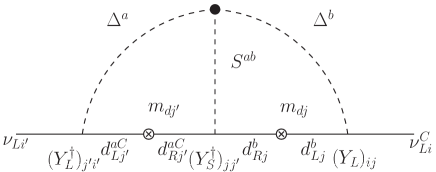
Figure 1: The 2-loop neutrino mass generated from colored scalar. Where $a,b,c$ are the $SU(3)$ indices.

However, the simultaneous presence of $Y_{L/R}$ and $y^{\Delta}$ leads to tree-level proton decay as pointed out in LQ-Wise . A very small $y^{\Delta}_{11}$ is enough to avoid the rapid proton decay problem. Alternatively, the $y^{\Delta}$ term can be eliminated by imposing some ad hoc symmetry. For example, this term can be turned off without upsetting all other interactions if some $Z_{2}$ parities $\{-,-,+,+,+,-,+\}$ are assigned to $\{L,l_{R},Q,u_{R},d_{R},\Delta,S\}$, respectively. Hence, we leave the proton decay problem aside and simply set $y^{\Delta}=0$ in this study.

The most general renormalizable scalar potential including $S$ and $\Delta$ is

$$\mathscr{V} = -\mu_{H}^{2}(H^{\dagger}H)+m_{\Delta}^{2}\Delta^{\dagger}\Delta+m_{S}^{2}\mbox{Tr}S^{\dagger}S+\lambda(H^{\dagger}H)^{2}+\lambda_{\Delta}(\Delta^{\dagger}\Delta)^{2}+\lambda_{S}(\mbox{Tr}S^{\dagger}S)^{2}$$

$$+\lambda_{1}(\Delta^{\dagger}\Delta)(H^{\dagger}H)+\lambda_{2}\mbox{Tr}(S^{\dagger}S)(H^{\dagger}H)+\lambda_{3}\mbox{Tr}(S^{\dagger}S)(\Delta^{\dagger}\Delta)+\left(\mu\Delta^{*}\Delta^{*}S+h.c.\right)$$

where the trace is over the color indices. The details of the scalar potential are not relevant for the later discussion. We note by passing that only the SM Higgs doublet can acquire a nonzero vacuum expectation value, $\langle H\rangle=v/\sqrt{2}$, and being solely responsible for the electroweak symmetry breaking(EWSB). The tree-level masses of $\Delta$ and $S$ are shifted after EWSB with $m_{\Delta}^{2}\rightarrow m_{\Delta}^{2}+\lambda_{1}v^{2}/2$ and $m_{S}^{2}\rightarrow m_{S}^{2}+\lambda_{2}v^{2}/2$. To proceed, we need $m_{\Delta}$ and $m_{S}$ after EWSB as input. Since $S$ and $\Delta$ participate strong interactions, they are best searched for at the hadron colliders but so far none has been found yet. Depending on their couplings to the SM fields, some lower bounds on $m_{S}$ and $m_{\Delta}$ were obtained from the null result of collider searches. The current lower bounds on $m_{\Delta}$ are summarized in Table.1.

Table 1: Summary of leptoquark mass lower bound (in unit of $\mathrm{GeV}$) from direct search with $95\%$ CL. The values in parentheses are for $\beta=0.5$, and $\beta=1$ otherwise. The leptoquark decays branching ratios into $lq$ and $\nu q$ are denoted as $\beta$ and $(1-\beta)$, respectively, and $\lambda$ is the Yukawa coupling for $lq\Delta$. The leptoquark is assumed to decay into leptons within only one specific generation.

	First generation	Second generation	Third generation
CMS	$1005(845)$ CMS-1st	$1070(785)$ CMS-2nd	$634$ CMS-3rd
ATLAS	$660(607)$ ATLAS-1st	$685(594)$ ATLAS-2nd	$534$ ATLAS-3rd
ZEUS	$699(\lambda=0.3)$HERA-1st

For an $E_{6}$-type diquark, CMS study gives $m_{S}>6\mathrm{TeV}$ DQ-mass . These limits are very sensitive to the assumptions of decay branching fraction as well as the flavor dependant coupling strengthes. Hence, in the following numerically analysis, we take $m_{S}=7\,\mathrm{TeV}$ and $m_{\Delta}=1\,\mathrm{TeV}$ as the benchmark values.

The triple $\Delta\Delta S$ coupling generates 1-loop correction $\sim\frac{\mu^{2}}{16\pi^{2}}\log(\mu^{2}/m_{X}^{2})$ to $m_{X}^{2}$ where $X=S,\Delta$. For these quantum corrections to be perturbative, one needs roughly $|\mu^{2}\log(\mu^{2}/m_{X}^{2})|\leq 16\pi^{2}m_{X}^{2}$ . On the other hand, the dimensionful parameters in the same scalar potential are expected to be around the same order. These considerations led to similar estimations and $\mu=(0.1-1)\,{\rm{TeV}}$ is assumed in this study.

At the tree-level, the decay channels for leptoquark are $\Delta\rightarrow\ell_{i}u_{j}$ and $\Delta\rightarrow\nu_{i}d_{j}$. For di-quark, it decays into $d_{i}d_{j}$, and $\Delta\Delta$ if kinematically allowed. Given that $m_{S},m_{\Delta}\gg m_{t}$, all the SM final states can be treated massless and the decay widthes can be calculated to be

$$\Gamma_{\Delta} = \sum_{i,j}\left[\Gamma(\Delta\rightarrow\ell_{i}u_{j})+\Gamma(\Delta\rightarrow\nu_{i}d_{j})\right]\sim\frac{m_{\Delta}}{16\pi}\sum_{i,j}\left(2|(Y_{L})_{ij}|^{2}+|(Y_{R})_{ij}|^{2}\right)\,,$$ (11)

$$\Gamma_{S} = \Gamma(S\rightarrow\Delta\Delta)\times\theta(m_{S}-2m_{\Delta})+\sum_{ij}\Gamma(S\rightarrow d_{i}d_{j})$$ (12)

$$\sim \frac{m_{S}}{8\pi}\left\{\left(1-4\frac{m^{2}_{\Delta}}{m_{S}^{2}}\right)^{1/2}\left(\frac{\mu}{m_{S}}\right)^{2}\times\theta(m_{S}-2m_{\Delta})+\sum_{i,j}|(Y_{S})_{ij}|^{2}\right\}.$$

3 Neutrino Masses and the Tree-level Flavor Violation

As discussed before, it is assumed that there is no hierarchy among the $Y_{S}$’s. Since $m_{b}\gg m_{s}\gg m_{d}$, the matrix $\omega$ can be broken into the leading and sub-leading parts and $\omega=\omega^{(0)}+\omega^{(1)}$, where

$$\omega^{(0)}=24\mu I_{\nu}\times\left(\begin{array}[]{ccc}0&0&0\\ 0&0&m_{b}m_{s}(Y_{S})_{23}^{*}\\ 0&m_{b}m_{s}(Y_{S})_{23}^{*}&m_{b}^{2}(Y_{S})_{33}^{*}\end{array}\right)\,,$$ (13)

and ${\cal O}\left(\frac{\omega^{(1)}}{\omega^{(0)}}\right)\sim{\cal O}\left(\frac{m_{d}}{m_{b}}\right)$. It is easy to check that the leading neutrino mass matrix $M_{\nu}^{(0)}=Y_{L}\omega^{(0)}Y_{L}^{T}$ is of rank-2 and $\det M_{\nu}^{(0)}=0$. Hence, at least one of the active neutrinos is nearly massless, $\sim(m_{d}/m_{b})\times\mbox{max}(m_{\nu})$, and the scenario of quasi-degenerate neutrinos is disfavored in the cZBM. At leading order, $(Y_{L})_{11,21,31}$ do not enter $M_{\nu}^{(0)}$ at all. Therefor, for either normal hierarchy (NH) or the inverted hierarchy(IH) type of the neutrino masses, the eigenmasses are

• NH:

  $$m_{1}\simeq 0\,,m_{2}\simeq\sqrt{\Delta m_{21}^{2}}\,,m_{3}\simeq\sqrt{\Delta m^{2}+\frac{\Delta m_{21}^{2}}{2}}\,,$$ (14)

  and

• IH:

  $$m_{3}\simeq 0\,,m_{1}\simeq\sqrt{|\Delta m^{2}|-\frac{\Delta m_{21}^{2}}{2}}\,,m_{2}\simeq\sqrt{|\Delta m^{2}|+\frac{\Delta m_{21}^{2}}{2}}\,,$$ (15)

where $\Delta m^{2}\equiv m_{3}^{2}-(m_{1}^{2}+m_{2}^{2})/2$. Moreover, the absolute values of neutrino mass can be obtained by plugging in the well determined neutrino dataPDG listed in Table 2. For NH, $m_{2}\sim 0.00868$ eV and $m_{3}\sim 0.0496$ eV, and for IH, $m_{1}\sim 0.0483$ eV and $m_{2}\sim 0.0492$ eV. For both cases, the total sum of neutrino masses automatically agrees with the limit that $\sum m_{\nu}<0.23$ eV at $95\%$ C.L. from the cosmological observationnu-mass .

Table 2: The global-fit neutrino data with $1\sigma$ deviationPDG .

$\sin^{2}\theta_{23}$	$0.437^{+0.033}_{-0.023}$  (NH)
	$0.455^{+0.039}_{-0.031}$  (IH)
$\sin^{2}\theta_{13}$	$0.0234^{+0.0020}_{-0.0019}$ (NH)
	$0.0240^{+0.0019}_{-0.0022}$  (IH)
$\sin^{2}\theta_{12}$	$0.308^{+0.017}_{-0.017}$
$\Delta m_{21}^{2}$	$\left(7.54^{+0.26}_{-0.22}\right)\times 10^{-5}\mathrm{eV}^{2}$
$|\Delta m^{2}|$	$\left(2.43^{+0.06}_{-0.06}\right)\times 10^{-3}\mathrm{eV}^{2}$  (NH)
	$\left(2.38^{+0.06}_{-0.06}\right)\times 10^{-3}\mathrm{eV}^{2}$  (IH)
$\delta/\pi$	$1.39^{+0.38}_{-0.27}$  (NH)
	$1.31^{+0.29}_{-0.33}$  (IH)

Once $m_{1,2,3}$ are fixed, the neutrino mass matrix can be worked out reversely by

$$M_{\nu}=U_{PMNS}^{*}\left(\begin{array}[]{ccc}m_{1}&0&0\\ 0&m_{2}&0\\ 0&0&m_{3}\end{array}\right)U_{PMNS}^{\dagger}\,.$$ (16)

The standard parametrization is adopted that

$$U_{\mathrm{PMNS}}=\left(\begin{array}[]{ccc}1&0&0\\ 0&c_{23}&s_{23}\\ 0&-s_{23}&c_{23}\end{array}\right)\left(\begin{array}[]{ccc}c_{13}&0&s_{13}e^{-i\delta}\\ 0&1&0\\ -s_{13}e^{i\delta}&0&c_{13}\end{array}\right)\left(\begin{array}[]{ccc}c_{12}&s_{12}&0\\ -s_{12}&c_{12}&0\\ 0&0&1\end{array}\right)\begin{pmatrix}1&0&0\\ 0&e^{i\alpha_{21}/2}&0\\ 0&0&e^{i\alpha_{31}/2}\end{pmatrix}$$ (17)

where $c_{ij}$ and $s_{ij}$ represent $\cos\theta_{ij}$ and $\sin\theta_{ij}$, respectively. In the case of Majorana neutrinos, $\alpha_{21}$ and $\alpha_{31}$ are the extra CP phases that cannot be determined from the oscillation experiments. For simplicity, all $Y_{S}$’s are assumed to be real and the 2 Majorana CP phases will not be discussed in this paper. The leading order neutrino mass matrix has 5(=6-1) independent entries. With the democratic $Y_{S}$ assumption, the effective Majorana mass for $(\beta\beta)_{0\nu}$-decay $m_{ee}\sim 0.0018$ eV for the NH case. For the IH case, $m_{ee}\sim 0.0479$ eV which is within the sensitivity of the planned $(0\nu\beta\beta)$ detectors with $\sim 1$ ton of isotopeBilenky:2012qi . Furthermore, the lightest neutrino mass is $\sim{\cal O}(10^{-5}\mbox{eV})$ for both IH and NH cases. For a given set of parameters, $\{\mu,m_{S},m_{\Delta},(Y_{S})^{(0)}_{23},(Y_{S})^{(0)}_{33},(Y_{L})_{13}\}$, all the other 5 complex Yukawa couplings $(Y_{L})_{ij}(j\neq 1)$ can be completely determined up to two signs by the leading $M_{\nu}^{(0)}$. For a real $(Y_{L})_{13}$, one has

$$(Y_{L})_{23}^{(0)} = \frac{(Y_{L})_{13}}{(M_{\nu})_{11}}\left[(M_{\nu})_{12}\pm\sqrt{(M_{\nu})_{12}^{2}-(M_{\nu})_{11}(M_{\nu})_{22}}\right]\,,$$

$$(Y_{L})_{33}^{(0)} = \frac{(Y_{L})_{13}}{(M_{\nu})_{11}}\left[(M_{\nu})_{13}\pm\sqrt{(M_{\nu})_{13}^{2}-(M_{\nu})_{11}(M_{\nu})_{33}}\right]\,,$$

$$(Y_{L})_{12}^{(0)} = {(M_{\nu})_{11}-B_{\nu}m_{b}^{2}(Y_{L})_{13}^{2}(Y_{S})_{33}^{(0)}\over 2B_{\nu}m_{b}m_{s}(Y_{L})_{13}(Y_{S})_{23}^{(0)}}\,,$$

$$(Y_{L})_{22}^{(0)} = {(M_{\nu})_{22}-B_{\nu}m_{b}^{2}[(Y_{L})_{23}^{(0)}]^{2}(Y_{S})_{33}^{(0)}\over 2B_{\nu}m_{b}m_{s}(Y_{L})_{23}^{(0)}(Y_{S})_{23}^{(0)}}\,,$$

$$(Y_{L})_{32}^{(0)} = {(M_{\nu})_{33}-B_{\nu}m_{b}^{2}[(Y_{L})_{33}^{(0)}]^{2}(Y_{S})_{33}^{(0)}\over 2B_{\nu}m_{b}m_{s}(Y_{L})_{33}^{(0)}(Y_{S})_{23}^{(0)}}\,,$$ (18)

where $B_{\nu}=24\mu I_{\nu}$. Again, $(Y_{L})_{11,21,31}$ do not enter $M_{\nu}^{(0)}$ at all; they are arbitrary at this level and will be determined in the next order perturbation. This approximation largely saves the work of numerical study and lays out the base for higher order perturbations beyond $\omega^{(0)}$.

The most important next to leading contribution to $M_{\nu}$ comes from $(Y_{S})_{13}$. If one also perturbs $(Y_{S})_{23,33}$ around $(Y_{S})^{(0)}_{23,33}$ with $(Y_{S})_{23,33}^{(1)}=(Y_{S})^{(0)}_{23,33}+\delta_{23,33}$, the consistent solution to $(Y_{L})_{i1}$ for a given set $\{(Y_{S})_{13},\delta_{23},\delta_{33}\}$ are:

$$(Y_{L})_{11}^{(1)} = -\frac{m_{s}}{m_{d}}\frac{\delta_{23}}{(Y_{S})_{13}}(Y_{L})_{12}^{(0)}-\frac{m_{b}}{2m_{d}}\frac{\delta_{33}}{(Y_{S})_{13}}(Y_{L})_{13}\,,$$

$$(Y_{L})_{21}^{(1)} = -\frac{m_{s}}{m_{d}}\frac{\delta_{23}}{(Y_{S})_{13}}(Y_{L})_{22}^{(0)}-\frac{m_{b}}{2m_{d}}\frac{\delta_{33}}{(Y_{S})_{13}}(Y_{L})_{23}^{(0)}\,,$$

$$(Y_{L})_{31}^{(1)} = -\frac{m_{s}}{m_{d}}\frac{\delta_{23}}{(Y_{S})_{13}}(Y_{L})_{32}^{(0)}-\frac{m_{b}}{2m_{d}}\frac{\delta_{33}}{(Y_{S})_{13}}(Y_{L})_{33}^{(0)}\,.$$ (19)

With only a handful of free parameters, all the leptoquark left-handed Yukawa can be reasonably determined solely by the neutrino data. However, further checks are needed to determine whether the above solution is phenomenologically viable. Next, the tree-level flavor violation will be discussed.

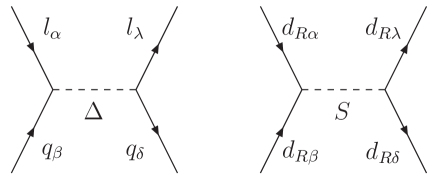
Figure 2: Tree-level flavor violation mediated by leptoquark and diquark.

The leptonic and quark flavor violating processes will be generated by exchanging $S$ and $\Delta$ at the tree-level, see Fig.2. Since $S,\Delta$ are heavy, they can be integrated out below the EWSB scale. After Fierz transformation, we obtain

$$\begin{aligned} \triangle\mathcal{L}_{\mbox{eff}}=&\left[\frac{(Y_{L}^{*})_{ml}(Y_{R})_{ij}}{2m_{\Delta}^{2}}\left(-\overline{\nu_{m}}\mathbb{P}_{R}\ell_{i}\cdot\overline{d_{l}^{a}}\mathbb{P}_{R}u_{j}^{a}+\overline{\ell_{m}}\mathbb{P}_{R}\ell_{i}\cdot\overline{u_{l}^{a}}\mathbb{P}_{R}u_{j}^{a}\right)+h.c.\right]\\ &-\left[\frac{(Y_{L}^{*})_{ml}(Y_{L})_{ij}}{2m_{\Delta}^{2}}\overline{\nu_{m}}\gamma^{\mu}\mathbb{P}_{L}\ell_{i}\cdot\overline{d_{l}^{a}}\gamma_{\mu}\mathbb{P}_{L}u_{j}^{a}+h.c.\right]\\ &+\frac{(Y_{L}^{*})_{ml}(Y_{L})_{ij}}{2m_{\Delta}^{2}}\left(\overline{\nu_{m}}\gamma^{\mu}\mathbb{P}_{L}\nu_{i}\cdot\overline{d_{l}^{a}}\gamma_{\mu}\mathbb{P}_{L}d_{j}^{a}+\overline{\ell_{m}}\gamma^{\mu}\mathbb{P}_{L}\ell_{i}\cdot\overline{u_{l}^{a}}\gamma_{\mu}\mathbb{P}_{L}u_{j}^{a}\right)\\ &+\frac{(Y_{R}^{*})_{ml}(Y_{R})_{ij}}{2m_{\Delta}^{2}}\overline{\ell_{m}}\gamma^{\mu}\mathbb{P}_{R}\ell_{i}\cdot\overline{u_{l}^{a}}\gamma_{\mu}\mathbb{P}_{R}u_{j}^{a}\\ &+\left[\frac{(Y_{L}^{*})_{ml}(Y_{R})_{ij}}{8m_{\Delta}^{2}}\left(\overline{\nu_{Lm}}\sigma^{\mu\nu}\mathbb{P}_{R}\ell_{i}\cdot\overline{d_{l}^{a}}\sigma_{\mu\nu}\mathbb{P}_{R}u_{j}^{a}-\overline{\ell_{Lm}}\sigma^{\mu\nu}\mathbb{P}_{R}\ell_{i}\cdot\overline{u_{l}^{a}}\sigma_{\mu\nu}\mathbb{P}_{R}u_{j}^{a}\right)+h.c.\right]\\ &+\frac{(Y_{s})_{ij}(Y_{s}^{\dagger})_{lm}}{2m_{S}^{2}}\left[\overline{d_{m}^{a}}\gamma^{\mu}\mathbb{P}_{\!\scriptscriptstyle R}d_{i}^{a}\right]\left[\overline{d_{l}^{b}}\gamma_{\mu}\mathbb{P}_{\!\scriptscriptstyle R}d_{j}^{b}\right]\end{aligned}$$ (20)

where $a,b$ are the color indices.

There are way too many new free parameters and rich phenomenology in the most general model. To simplify the discussion and to extract the essential physics, we consider the case that the new physics has minimal tree-level flavor violation(TLFV). Note that the TLFV contributions from different chiral structures always add incoherently. To minimize the total TLFV we need to suppress the TLFV from each chiral structure as much as possible. Let’s concentrate on the purely left-handed operators first. Observe that (1) A trivial flavor violation free solution is that with $(Y_{L})_{ij}(Y_{L}^{\dagger})_{lm}\propto\delta_{im}\delta_{jl}$. It is obvious that these kind of solutions allow only one nonzero entry of $Y_{L}$, as can be easily seen by looking at Fig.2(a). It always leads to 2 massless neutrinos which has been excluded by the current neutrino oscillation data. (2) If the requirement is relaxed to $(Y_{L})_{ij}(Y_{L}^{\dagger})_{lm}\propto\delta_{im}$ (no leptonic TLFV) or $(Y_{L})_{ij}(Y_{L}^{\dagger})_{lm}\propto\delta_{jl}$ ( no quark TLFV), only one row or one column of $Y_{L}$ can be nonzero and the resulting neutrino masses have two zeros again. However, only $Y_{L}$’s are relevant to the neutrino masses. One can set $Y_{R}=0$ to minimize the TLFV, and use the 9 remaining $Y_{L}$’s to accommodate the neutrino masses. Then the lower bound on each flavor violation process can be found since any nonzero $Y_{R}$ will add to it.

It is very easy to build a model with $Y_{R}\ll 1$ or $Y_{R}=0$ and we supplement with two examples. Example one is to introduce an extra $U(1)_{x}$ with two SM like Higgs doublets, $H_{1}$ and $H_{2}$. Then the $U(1)_{x}$ charge assignment $\{\alpha_{1},\alpha_{2},\alpha_{2},\alpha_{3},\alpha_{4},\alpha_{5},\alpha_{6},\alpha_{7}\}$ for $\{Q,u_{R},d_{R},L,e_{R},H_{1},H_{2},\Delta\}$ with $\alpha_{5}=\alpha_{1}-\alpha_{2}$, $\alpha_{6}=\alpha_{3}-\alpha_{4}$, $\alpha_{7}=-(\alpha_{1}+\alpha_{3})$, $\alpha_{7}\neq 2\alpha_{2}$ and $\alpha_{7}\neq(\alpha_{2}+\alpha_{4})$ will kill $Y_{R}$ (and also $y^{\Delta}$) but still allow the charged fermions to acquire the Dirac masses from their Yukawa couplings with $H_{1}$ or $H_{2}$. There are other issues needed to be considered in this setup. For example whether the $U(1)_{x}$ is global or local and whether it is free of anomaly. But these issues do not concern us since they are not relevant to this study and there are well-known model-building machineries available to deal with these problems. The second example is promoting the 4-dimensional model into a higher-dimensional version. If the wave functions of $l_{R}$ and $u_{R}$ in the extra spacial dimension(s) are well separated, like in Chang:SF , or have very little overlapping, like inChang:RS , the resulting $Y_{R}$ is negligible. Anyway, here $Y_{R}=0$ is taken as a phenomenology assumption which minimizes the TLFV. Some remarks on the case of $Y_{R}\neq 0$ will be discussed in next section.

A model independent analysis of the effective four-fermion operators was done by2L2Q . The $90\%$ C.L. upper limits on the normalized Wilson coefficient $\epsilon_{ijkl}$ (it is not the totally anti-symmetric tensor),

$$\epsilon_{ijkn}\equiv\frac{(Y_{L})_{ik}(Y_{L})_{jn}}{4\sqrt{2}G_{F}m_{\Delta}^{2}}\,,$$ (21)

for each 4-fermi operator are extracted and listed in Table 3. We have

$$(Y_{L})_{ik}(Y_{L})_{jn}<4\sqrt{2}G_{F}m_{\Delta}^{2}\epsilon_{ijkn}^{\text{max}}\sim 65.98\times\epsilon_{ijkn}^{\text{max}}\times\left({m_{\Delta}\over 1\mbox{TeV}}\right)^{2}\,.$$ (22)

Table 3: The 90%C.L. upper limits on $\epsilon_{ijkn}$ from 2L2Q . Here, the dimensionless quantities $\epsilon_{ijkn}\equiv(Y_{L})_{ik}(Y_{L})_{jn}/(4\sqrt{2}G_{F}m_{\Delta}^{2})$, where $i,j$($k,n$)are lepton(quark) flavor indices.

$\epsilon_{ee11}$	$10^{-3}$	$\epsilon_{ee12}$	$9.4\times 10^{-6}$	$\epsilon_{ee13}$	$3.9\times 10^{-3}$
$\epsilon_{ee22}$	$10^{-2}$	$\epsilon_{ee23}$	$10^{-3}$	$\epsilon_{ee33}$	$9.2\times 10^{-2}$
$\epsilon_{\mu\mu 11}$	$7.3\times 10^{-3}$	$\epsilon_{\mu\mu 12}$	$9.4\times 10^{-6}$	$\epsilon_{\mu\mu 13}$	$3.9\times 10^{-3}$
$\epsilon_{\mu\mu 22}$	$1.2\times 10^{-1}$	$\epsilon_{\mu\mu 23}$	$10^{-3}$	$\epsilon_{\mu\mu 33}$	$6.1\times 10^{-2}$
$\epsilon_{\tau\tau 11}$	$10^{-2}$	$\epsilon_{\tau\tau 12}$	$9.4\times 10^{-6}$	$\epsilon_{\tau\tau 13}$	$3.9\times 10^{-3}$
$\epsilon_{\tau\tau 22}$	$1.2\times 10^{-1}$	$\epsilon_{\tau\tau 23}$	$10^{-3}$	$\epsilon_{\tau\tau 33}$	$8.6\times 10^{-2}$
$\epsilon_{e\mu 11}$	$8.5\times 10^{-7}$	$\epsilon_{e\mu 12}$	$9.4\times 10^{-6}$	$\epsilon_{e\mu 13}$	$3.9\times 10^{-3}$
$\epsilon_{e\mu 21}$	$9.4\times 10^{-6}$	$\epsilon_{e\mu 22}$	$0.24$	$\epsilon_{e\mu 23}$	$10^{-3}$
$\epsilon_{e\mu 31}$	$3.9\times 10^{-3}$	$\epsilon_{e\mu 32}$	$10^{-3}$	$\epsilon_{e\mu 33}$	$6.6\times 10^{-2}$
$\epsilon_{e\tau 11}$	$8.4\times 10^{-4}$	$\epsilon_{e\tau 12}$	$9.4\times 10^{-6}$	$\epsilon_{e\tau 13}$	$3.9\times 10^{-3}$
$\epsilon_{e\tau 21}$	$9.4\times 10^{-6}$	$\epsilon_{e\tau 22}$	$0.24$	$\epsilon_{e\tau 23}$	$10^{-3}$
$\epsilon_{e\tau 31}$	$3.9\times 10^{-3}$	$\epsilon_{e\tau 32}$	$10^{-3}$	$\epsilon_{e\tau 33}$	$0.2$
$\epsilon_{\mu\tau 11}$	$9.4\times 10^{-4}$	$\epsilon_{\mu\tau 12}$	$9.4\times 10^{-6}$	$\epsilon_{\mu\tau 13}$	$3.9\times 10^{-3}$
$\epsilon_{\mu\tau 21}$	$9.4\times 10^{-6}$	$\epsilon_{\mu\tau 22}$	$0.24$	$\epsilon_{\mu\tau 23}$	$10^{-3}$
$\epsilon_{\mu\tau 31}$	$3.9\times 10^{-3}$	$\epsilon_{\mu\tau 32}$	$10^{-3}$	$\epsilon_{\mu\tau 33}$	$1$

For the TLFV mediated by $S$, the last term in Eq.(20), it is best constrained by the neutral meson mixings. Following the convention in UTfit , the corresponding Wilson coefficients and the 4-fermi operators for $K$-$\bar{K}$, $B_{d}$-$\bar{B}_{d}$ and $B_{s}$-$\bar{B}_{s}$ mixing are

$$\tilde{C}^{1}_{K}=-\frac{1}{2m_{S}^{2}}(Y_{s})_{11}(Y_{s}^{\dagger})_{22},\quad\tilde{Q}^{1}_{K}=(\bar{s}\gamma^{\mu}\mathbb{P}_{\!\scriptscriptstyle R}d)(\bar{s}\gamma_{\mu}\mathbb{P}_{\!\scriptscriptstyle R}d)\,,$$

$$\tilde{C}^{1}_{B}=-\frac{1}{2m_{S}^{2}}(Y_{s})_{11}(Y_{s}^{\dagger})_{33},\quad\tilde{Q}^{1}_{B}=(\bar{b}\gamma^{\mu}\mathbb{P}_{\!\scriptscriptstyle R}d)(\bar{b}\gamma_{\mu}\mathbb{P}_{\!\scriptscriptstyle R}d)\,,$$

$$\tilde{C}^{1}_{B_{s}}=-\frac{1}{2m_{S}^{2}}(Y_{s})_{22}(Y_{s}^{\dagger})_{33},\quad\tilde{Q}^{1}_{B_{s}}=(\bar{b}\gamma^{\mu}\mathbb{P}_{\!\scriptscriptstyle R}s)(\bar{b}\gamma_{\mu}\mathbb{P}_{\!\scriptscriptstyle R}s)\,.$$ (23)

A global analysis with $95\%$ C.L. gaveUTfit

$$|\mathrm{Re}(\tilde{C}_{K}^{1})|<9.6\times 10^{-13},\quad-4.4\times 10^{-15}<\mathrm{Im}(\tilde{C}_{K}^{1})<2.8\times 10^{-15}\,,$$

$$|\tilde{C}_{B_{d}}^{1}|<2.3\times 10^{-11},\quad-\pi<\mathrm{Arg}(\tilde{C}_{B_{d}}^{1})<\pi\,,$$

$$|\tilde{C}_{B_{s}}^{1}|<1.1\times 10^{-9},\quad-\pi<\mathrm{Arg}(\tilde{C}_{B_{s}}^{1})<\pi\,,$$ (24)

in the unit of $\mathrm{GeV}^{-2}$. Or equivalently,

$$|(Y_{s})_{11}(Y_{s})^{\dagger}_{22}|<1.92\times 10^{-6}\times\left(\frac{m_{S}}{\text{TeV}}\right)^{2},$$

$$|(Y_{s})_{11}(Y_{s})^{\dagger}_{33}|<4.6\times 10^{-5}\times\left(\frac{m_{S}}{\text{TeV}}\right)^{2},$$

$$|(Y_{s})_{22}(Y_{s})^{\dagger}_{33}|<2.2\times 10^{-3}\times\left(\frac{m_{S}}{\text{TeV}}\right)^{2}.$$ (25)

For the democratic $Y_{S}$, the above constraints imply $|Y_{S}|\lesssim 9\times 10^{-3}\times(m_{S}/7\mbox{TeV})$.

Before ending this section, we recap the assumptions and discussion so far:

• $Y_{S}$’s are assumed to be democratic and there is no outstanding hierarchy among these Yukawa couplings. This leads to one nearly massless active neutrino and $|Y_{S}|\lesssim 9\times 10^{-3}\times(m_{S}/7\mbox{TeV})$ from the constrains of neutral meson mixings.

• The Yukawa couplings $Y_{R}$ are turned off to minimize the TLFV.

• For a given set of $\{\mu,m_{S},m_{\Delta},(Y_{S})_{13,23,33}\}$ and any one of the $Y_{L}$’s, all the remaining 8 $Y_{L}$ can be iteratively determined from the absolute neutrino masses and the $U_{PMNS}$ matrix.

4 Charged lepton flavor violating process at one-loop

In this section, we shall study the charged lepton flavor violating (cLFV) processes $\ell\to\ell^{\prime}\gamma$, $Z\to\ell^{\prime}\bar{\ell}$ and the like which are induced at the 1-loop level with the leptoquark running in the loop, see Fig.3.

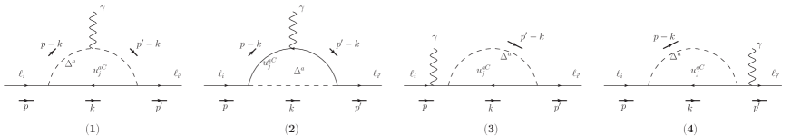
Figure 3: The Feynman diagrams for 1-loop LFV $\mu\to e\gamma$.

4.1 $\ell\to\ell^{\prime}\gamma$

The effective Lagrangian responsible for the cLFV process $\ell\to\ell^{\prime}\gamma$Kuno ; WFC-LFV is parameterized as

$$\mathscr{L}\supset\frac{1}{2}\bar{\ell}^{\prime}\left(d_{L}^{ll^{\prime}}\mathbb{P}_{\!\scriptscriptstyle L}+d_{R}^{ll^{\prime}}\mathbb{P}_{\!\scriptscriptstyle R}\right)\sigma^{\mu\nu}\ell F_{\mu\nu}+h.c.$$ (26)

For $m_{\ell}^{\prime}\ll m_{\ell}$, the partial decay width is given as

$$\Gamma(\ell\to\ell^{\prime}\gamma)\simeq{m_{\ell}^{3}\over 16\pi}(|d^{ll^{\prime}}_{L}|^{2}+|d^{ll^{\prime}}_{R}|^{2})\,.$$ (27)

A straightforward calculation yields

$$d_{R}^{ll^{\prime}}=-{N_{c}e\over 16\pi^{2}m_{\Delta}^{2}}\left[\left(m_{l^{\prime}}(Y^{*}_{R})_{l^{\prime}q}(Y^{T}_{R})_{ql}+m_{l}(Y^{*}_{L})_{l^{\prime}q}(Y^{T}_{L})_{ql}\right){\cal F}_{1}(r_{q})+m_{q}(Y^{*}_{L})_{l^{\prime}q}(Y^{T}_{R})_{ql}{\cal F}_{2}(r_{q})\right]\,,$$ (28)

where the index $q$ sums over $q=u,c,t$ and $r_{q}\equiv m_{q}^{2}/m_{\Delta}^{2}$. $d_{L}^{ll^{\prime}}$ can be obtained by simply switching $Y_{L}\leftrightarrow Y_{R}$ in the above expression for $d_{R}^{ll^{\prime}}$. The loop functions are

$${\cal F}_{1}(x) = {1+4x-5x^{2}+2x(2+x)\ln x\over 12(1-x)^{4}}\,,$$

$${\cal F}_{2}(x) = {7-8x+x^{2}+2(2+x)\ln x\over 6(1-x)^{3}}\,,$$ (29)

and they take the limits ${\cal F}_{1}\rightarrow 1/12$ and ${\cal F}_{2}\rightarrow 7/6+(2\ln x)/3$ when $x\rightarrow 0$. Unlike at the tree-level, the contributions to the cLFV processes from $Y_{L}$ and $Y_{R}$ entangle with each other at the loop-level. Since $m_{q}{\cal F}_{2}(r_{q})\gg m_{l}{\cal F}_{1}(r_{q})$ (for $q=c,t$), generally speaking, the last term in Eq.(28) which involves both $Y_{L}$ and $Y_{R}$ gives the most important contribution to $d_{R}^{ll^{\prime}}$. Therefore, it is expected that by setting $Y_{R}=0$ to minimize the TLFV will also reduce the 1-loop cLFV processes in general. In the $Y_{R}=0$ case, $d_{R}^{ll^{\prime}}$ dominates the cLFV processes because $m_{\ell}\gg m_{\ell^{\prime}}$. With $\tau_{\mu}^{-1}\approx\Gamma(\mu\to e\bar{\nu}_{e}\nu_{\mu})=\frac{1}{192\pi^{3}}G_{F}^{2}m_{\mu}^{5}$ and $\Gamma_{\tau}=0.002265{\rm{GeV}}$, the branching ratios for $\ell\to\ell^{\prime}\gamma$ are

$$\mathcal{B}(\mu\to e\gamma)\simeq\frac{12\pi^{2}|d_{R}^{\mu e}|^{2}}{G_{F}^{2}m_{\mu}^{2}}\,,\,\,\mathcal{B}(\tau\to\ell^{\prime}\gamma)\simeq\frac{m_{\tau}^{3}|d_{R}^{\tau l^{\prime}}|^{2}}{16\pi\Gamma_{\tau}}\,.$$ (30)

and

$$d_{R}^{ll^{\prime}}=-\frac{eN_{c}m_{\ell}}{12(4\pi)^{2}m_{\Delta}^{2}}\sum_{q=u,c,t}\left[a_{q}^{\gamma}(Y_{L})^{*}_{\ell^{\prime}q}(Y_{L})_{\ell q}\right]\,,$$ (31)

where $a^{\gamma}_{q}=1+4r_{q}(\ln r_{q}+1)+{\cal O}(r_{q}^{2})$, $a^{\gamma}_{u}\sim a^{\gamma}_{c}\sim 1.0$ and $a^{\gamma}_{t}\sim 0.82$. Numerically, we have

$$\mathcal{B}(\mu\to e\gamma) \simeq 2.1\times 10^{-7}\times\left|\sum_{q=u,c,t}a_{q}^{\gamma}(Y_{L}^{*})_{eq}(Y_{L})_{\mu q}\right|^{2}\times\left({1\mbox{TeV}\over m_{\Delta}}\right)^{4}\,,$$

$$\mathcal{B}(\tau\to\ell^{\prime}\gamma) \simeq 3.8\times 10^{-8}\times\left|\sum_{q=u,c,t}a_{q}^{\gamma}(Y_{L}^{*})_{\ell^{\prime}q}(Y_{L})_{\tau q}\right|^{2}\times\left({1\mbox{TeV}\over m_{\Delta}}\right)^{4}\,.$$ (32)

4.2 Remark on other photon dipole induced processes

4.2.1 Anomalous magnetic dipole moment

Similar calculation with little modification can be carried over for the flavor diagonal cases. For the charged lepton, the anomalous magnetic dipole moment is

$$\triangle a_{\ell}=\frac{N_{c}}{6(4\pi)^{2}}\frac{m_{\ell}^{2}}{m_{\Delta}^{2}}\left|\sum_{q=u,c,t}a_{q}^{\gamma}(Y_{L})_{\ell q}\right|^{2}\,.$$ (33)

Assuming that $|(Y_{L})_{lq}|^{2}\sim{\cal O}(1)$ and $m_{\Delta}=1$ TeV, one has $\triangle a_{e}\sim 8.0\times 10^{-16}$, $\triangle a_{\tau}\sim 1.0\times 10^{-8}$, and $\triangle a_{\mu}\sim 3.0\times 10^{-11}$. Unless $m_{\Delta}\ll 1$TeV and all 3 $(Y_{L})_{\mu q}$ are sizable and in phase, $\triangle a_{\mu}$ in this model is too small to accommodate the observed discrepancy $a_{\mu}^{exp}-a_{\mu}^{th}=(2.39\pm 0.79)\times 10^{-9}$ at $1\sigma$ C.L.mu:g-2 . Moreover, the model predicts a tiny positive $\triangle a_{e}$ which goes against the direction of the observed value that $a_{e}^{exp}-a_{e}^{th}=-10.6(8.1)\times 10^{-13}$ at $1\sigma$ C.L.e:g-2 . Of course, a much larger $\triangle a_{\mu}$ is possible to explain to observed discrepancy between the experimental measured value and the theoretical prediction if $Y_{R}\neq 0.$

4.2.2 Electric dipole moments

If $Y_{R}\neq 0$, the 1-loop charged lepton electric dipole moment(EDM), $d_{\ell}\sim\frac{N_{c}}{16\pi^{2}}\frac{m_{t}}{m_{\Delta}^{2}}\mathbf{Im}[Y_{L}Y_{R}^{*}]$, could be large. For $m_{\Delta}=1{\rm{TeV}}$, $|Y_{L}|\sim|Y_{R}|\sim 0.01$, and the CP phase is of order one, the typical electron EDM is around $10^{-24}\,e$-cm which is already 4 orders of magnitude larger than the current limit $|d_{e}|<8.7\times 10^{-29}e$-cm e:edm . Then, how to suppress the EDM’s in this model will be a pressing theoretical issue. A plain solution is setting $m_{\Delta}\gtrsim 100{\rm{TeV}}$ to avoid the too large EDMs but the phenomenology at the low energies are strongly suppressed as well.

On the other hand, if $Y_{R}=0$ there is no EDM at the 1-loop level. In fact, the first non-zero EDM contribution we can construct begins at the 3-loop level and it involves both $V^{CKM}$ and $U^{PMNS}$. An order of magnitude estimate gives:

$$d_{\ell}\sim\frac{\alpha N_{c}}{(16\pi)^{3}}\frac{m_{\ell}}{m_{\Delta}^{2}}\mathbf{Im}\left[(Y_{L})_{\ell k}V^{CKM}_{kj}(Y_{L}^{\dagger})_{ji}U^{PMNS}_{i\ell}\right]\,.$$ (34)

If $Y_{L}$ takes a typical value $\sim 0.01$, $m_{\Delta}=1{\rm{TeV}}$, and the combined CP phase is $\sim{\cal O}(1)$, this 3-loop electron EDM is expected to be $|d_{e}|\lesssim 10^{-37}\,e$-cm. This upper bound is slightly larger than the estimated SM upper bound for $d_{e}$ but way below the sensitivity of any EDM measurement in the foreseeable future. Consequently, $d_{e}$ is a useful handle to test the $Y_{R}=0$ assumption in the cZBM: once the electron EDM was measured to be greater than $10^{-37}\,e$-cm, either the $Y_{R}=0$ assumption with $m_{\Delta}\sim{\cal O}({\rm{TeV}})$ must be abandoned or more new physics is needed to go beyond the cZBM.

4.2.3 $\mu-e$ conversion

The $\mu-e$ conversion(MEC) will be mediated by the leptoquark at the tree-level as shown in Fig.2. For $Y_{R}=0$, the relevant 4-fermi operator is

$$\frac{(Y_{L})^{*}_{eu}(Y_{L})_{\mu u}}{2m_{\Delta}^{2}}\overline{e}\gamma^{\mu}\mathbb{P}_{L}\mu\cdot\overline{u^{a}}\gamma_{\mu}\mathbb{P}_{L}u^{a}+h.c.$$ (35)

The cLFV photon dipole operator discussed in the previous section will also contribute to MEC with an expected relative magnitude $\sim(\alpha/16\pi^{2})^{2}$ comparing to the tree-level one. Following the analysis of WFC-LFV , a more quantitative estimate for the MEC rate is:

$$\mathcal{B}_{conv} \simeq \mathcal{C}_{conv}\left\{\left(\frac{\alpha Z}{16\sqrt{2}\pi G_{F}m_{\Delta}^{2}}\right)^{2}|\sum_{q}a^{\gamma}_{q}(Y_{L})^{*}_{eq}(Y_{L})_{\mu q}|^{2}\right.$$ (36)

$$\left.+\left(\frac{(2Z+N)}{4\sqrt{2}G_{F}m_{\Delta}^{2}}\right)^{2}|(Y_{L})^{*}_{eu}(Y_{L})_{\mu u}|^{2}\right\}$$

$$\simeq \mathcal{C}_{conv}\left\{8.9\times 10^{-11}Z^{2}|\sum_{q}a^{\gamma}_{q}(Y_{L})^{*}_{eq}(Y_{L})_{\mu q}|^{2}\right.$$

$$\left.+2.3\times 10^{-4}(2Z+N)^{2}|(Y_{L})^{*}_{eu}(Y_{L})_{\mu u}|^{2}\right\}\times\left[\frac{{\rm{TeV}}}{m_{\Delta}}\right]^{4}\ ,$$

where Z is the atomic number and N is the neutron number for a certain nucleus. The overall factor $\mathcal{C}_{conv}$ depends on the form factors of the nuclei and the momentum of the muon. For instance, $\mathcal{C}_{conv}({}^{48}_{22}Ti)=1.2\times 10^{-3}$2L2Q . As can be seen, the LFV photon dipole indeed has much smaller contribution to the MEC than the tree-level one.

4.2.4 $\mu\rightarrow 3e$

In this model, there are no tree-level contributions to the cLFV $\mu\rightarrow 3e$ decay. The $\mu\rightarrow 3e$ process is dominated by the cLFV photon dipole transition and its rate is much smaller than ${\cal B}(\mu\rightarrow e\gamma)$. As pointed out in Kuno ; WFC-LFV , the ratio of ${\cal B}(\mu\rightarrow 3e)$ to ${\cal B}(\mu\rightarrow e\gamma)$ is basically model-independent:

$${{\cal B}(\mu\rightarrow 3e)\over{\cal B}(\mu\rightarrow e\gamma)}\sim\frac{2\alpha}{3\pi}\left[\ln\frac{m_{\mu}}{m_{e}}-\frac{11}{8}\right]\simeq 0.019\,.$$ (37)

Similarly, with replacing the charged lepton masses, the ratios in the rare tau decays are

$${{\cal B}(\tau\rightarrow 3e)\over{\cal B}(\tau\rightarrow e\gamma)}\sim\frac{2\alpha}{3\pi}\left[\ln\frac{m_{\tau}}{m_{e}}-\frac{11}{8}\right]\simeq 0.011\,,$$

$${{\cal B}(\tau\rightarrow 3\mu)\over{\cal B}(\tau\rightarrow\mu\gamma)}\sim\frac{2\alpha}{3\pi}\left[\ln\frac{m_{\tau}}{m_{\mu}}-\frac{11}{8}\right]\simeq 0.002\,.$$ (38)

For the decay channels with different flavor final sates, one hasWFC-LFV

$${{\cal B}(\tau\rightarrow\mu ee^{+})\over{\cal B}(\tau\rightarrow e\gamma)}\sim\frac{2\alpha}{3\pi}\left[\ln\frac{m_{\tau}}{m_{e}}-\frac{3}{2}\right]\simeq 0.032\,,$$ (39)

$${{\cal B}(\tau\rightarrow e\mu\mu^{+})\over{\cal B}(\tau\rightarrow e\gamma)}\sim\frac{2\alpha}{3\pi}\left[\ln\frac{m_{\tau}}{m_{\mu}}-\frac{3}{2}\right]\simeq 0.0064\,.$$ (40)

The decay branching ratios $\tau\rightarrow\mu^{+}ee$ and $\tau\rightarrow\mu\mu e^{+}$ are negligible because they are doubly suppressed by two cLFV transition vertices.

4.3 $Z\to\bar{\ell}\ell^{\prime}$

The same Feynman diagrams in Fig.3 with photon replaced by $Z$ boson lead to cLFV $Z\rightarrow\bar{l}l^{\prime}$ decays. Since $Z$ is massive, it can also admit the vector or axial-vector couplings other than the dipole transition couplings as in the $l\rightarrow l^{\prime}\gamma$ cases. The most general gauge invariant $Z\rightarrow\bar{l}l^{\prime}$ amplitude is parameterized as:

$$i\mathscr{M}=ie\overline{u}(p^{\prime})\left[(c_{R}^{Z}\mathbb{P}_{\!\scriptscriptstyle R}+c_{L}^{Z}\mathbb{P}_{\!\scriptscriptstyle L})\left(-g_{\mu\nu}+\frac{q_{\mu}q_{\nu}}{m_{Z}^{2}}\right)\gamma^{\nu}+\frac{1}{m_{Z}}\left(d_{L}^{Z}\mathbb{P}_{\!\scriptscriptstyle L}+d_{R}^{Z}\mathbb{P}_{\!\scriptscriptstyle R}\right)(i\sigma_{\mu\nu}q^{\nu})\right]v(-p)\epsilon^{\mu}(q)\,,$$ (41)

where the 4-momentums are labeled as in Fig.3. From the above parametrization, the branching ratio can be easily calculated to be

$$\mathcal{B}(Z\to\overline{\ell}{\ell}^{\prime})=\frac{\alpha}{6}\frac{m_{Z}}{\Gamma_{Z}}\left[(|c_{L}^{Z}|^{2}+|c_{R}^{Z}|^{2})+\frac{1}{2}\left(|d_{L}^{Z}|^{2}+|d_{R}^{Z}|^{2}\right)\right]\ ,$$ (42)

and the experimentally measured value $\Gamma_{Z}=2.4952\pm 0.0023\mathrm{GeV}$PDG is used in our study.

The 4 dimensionless coefficients $c^{Z}_{R,L},d^{Z}_{R,L}$ can be obtained through a lengthy but straightforward calculation. The physics is rather simple and can be understood qualitatively. However, the full analytic results are not very illustrating and will not be presented here. Let’s focus on the $Y_{R}=0$ case to simplify the physics discussion. First of all, the masses of external charged leptons are much smaller than $m_{Z}$ and they can be treated massless. For $c_{R}^{Z}$, the coupling connects both left-handed fermions and there is no need to flip their chiralities. In the loop calculation, $m_{Z}$ and $m_{t}$ are the only two dimensionful quantities other than $m_{\Delta}$. So, by dimensional analysis we know that $c_{R}^{Z}\sim{\cal O}(\frac{N_{c}}{16\pi^{2}}\frac{m_{t}^{2}}{m_{\Delta}^{2}})$ (for top quark running in the loop) or $c_{R}^{Z}\sim{\cal O}(\frac{N_{c}}{16\pi^{2}}\frac{m_{Z}^{2}}{m_{\Delta}^{2}})$( for light quarks running in the loop). For the dipole couplings which connect fermions with different handiness, one external charged lepton mass insertion is needed to flip its chirality. Also, $m_{Z}$ sets the nature scale of the momentum transfer in this process. Therefore it is expected that in general $d^{Z}/c^{Z}_{R}\sim{\cal O}(\frac{m_{l}}{m_{Z}})$ or ${\cal O}(\frac{m_{l}^{\prime}}{m_{Z}})$. Thus, the contributions from $d_{L,R}^{Z}$ can be safely ignored. On the other hand, both of the two external charged leptons need to flip their chiralities for having a nonzero $c_{L}^{Z}$ if $Y_{R}=0$. Therefore, $c_{L}^{Z}\sim{\cal O}(\frac{m_{l}m_{l}^{\prime}}{m_{Z}^{2}})c_{R}^{Z}$ and its contribution is totally negligible in this process. The above qualitative understandings agree very well with our full calculation. Hence, only the leading contribution from $c^{Z}_{R}$ is kept in the study. It is more useful to express the final result in the numerical form:

$$\mathcal{B}(Z\to\bar{\ell}\ell^{\prime})\simeq 1.46\times 10^{-7}\left|\sum_{q=u,c,t}a^{Z}_{q}(Y_{L})^{*}_{\ell^{\prime}q}(Y_{L})_{\ell q}\right|^{2}\times\left(\frac{{\rm{TeV}}}{m_{\Delta}}\right)^{4}\,,$$ (43)

where $a_{u}^{Z}=a_{c}^{Z}\simeq-0.125-0.077\mathbf{i}=-0.1468e^{i31.63^{\circ}}$ and $a_{t}^{Z}=1$. The imaginary part of $a^{Z}_{u,c}$ comes from the pole of light-quark propagators in the loop when the light quarks are going on-shell in the $Z$ decay. Also note that this cLFV decay branching ratio is around $10^{-7}$ if the absolute square in Eq.(43) is of order unit. The ballpark estimate is below but close to the current experimental limitsPDG ; ATLAS-Zdecay-2014 .

The interference between the sub-diagrams with $u(c)$ and $t$ running in the loop makes the relative phases between $a_{u,c}^{Z}$ and $a_{t}^{Z}$ observable. This physical phase leads to CP violation and in general $\mathcal{B}(Z\to\bar{\ell}\ell^{\prime})\neq\mathcal{B}(Z\to\bar{\ell^{\prime}}\ell)$. FollowingZCP_Bernabeu ; ZCP_Rius , the CP asymmetries are quantified as:

$$\eta_{\ell\ell^{\prime}}\equiv\mathcal{B}(Z\to\bar{\ell}\ell^{\prime})-\mathcal{B}(Z\to\bar{\ell^{\prime}}\ell)\,.$$ (44)

In this model, we have numerically

$$\eta_{\ell\ell^{\prime}}\simeq(4.53\times 10^{-8})\times{\bf Im}\left[\left(Y^{\ell^{\prime}\ell}_{u}+Y^{\ell^{\prime}\ell}_{c}\right)(Y^{\ell^{\prime}\ell}_{t})^{*}\right]\times\left(\frac{{\rm{TeV}}}{m_{\Delta}}\right)^{4}\,,$$ (45)

where the shorthand notation $Y^{\ell^{\prime}\ell}_{q}\equiv(Y_{L})^{*}_{\ell^{\prime}q}(Y_{L})_{\ell q}$. Interestingly, due to the sizable CP phase, the CP asymmetries and the cLFV decay branching ratios are of the same order. Also, for the later convenience, we define $\mathcal{B}^{Z}_{\ell\ell^{\prime}}\equiv\mathcal{B}(Z\to\bar{\ell}\ell^{\prime})+\mathcal{B}(Z\to\ell\bar{\ell^{\prime}})$.

Before closing this section, we should point out a simple but useful scaling relationship between $Y_{S}$ and $Y_{L}$ in this model. Recall that the neutrino mass is proportional to $Y_{S}Y_{L}^{2}$. Therefore, if $Y_{S}$ is re-scaled by $Y_{S}\rightarrow\lambda^{-2}Y_{S}$, then $Y_{L}$ must goes like $Y_{L}\rightarrow\lambda Y_{L}$ to keep the neutrino mass unchanged. After such rescaling, ${\cal B}(\ell\rightarrow\ell^{\prime}\gamma)$, MEC, $\mathcal{B}^{Z}_{\ell\ell^{\prime}}$ and $\eta_{\ell\ell^{\prime}}$ go like $\lambda^{4}$ while $\epsilon_{ll^{\prime}qq^{\prime}}$, $\Delta a_{l}$, and EDM go like $\lambda^{2}$ due to their amplitude nature. This scaling relationship largely helps reduce the computer time in finding the realistic configurations.

Now we have everything needed for the numerical and phenomenological study.

5 Numerical Study

5.1 Scanning strategy

As discussed in Sec.3, once the set $\{\mu,m_{S},m_{\Delta},(Y_{S})_{13,23,33}\}$ plus any one out of the 9 $Y_{L}$’s are fixed, all the remaining 8 $Y_{L}$’s can be iteratively determined from the absolute neutrino masses and the $U_{PMNS}$ matrix. In our numerical search, we take $m_{\Delta}=1{\rm{TeV}}$ and $m_{S}=7{\rm{TeV}}$ as the benchmark. Moreover, for each configuration, $\mu$ is randomly produced within $[0.1,1]{\rm{TeV}}$. For each search, the neutrino mixings $sin^{2}\theta_{12,13,23}$, and the Dirac phase $\delta_{cp}$ are randomly generated within the 1 sigma allowed range from the global fit, Tab.2. For simplicity the two Majorana phases are set to be zero. Then the $U_{PMNS}$ matrix can be determined via Eq.(17). For a given $U_{PMNS}$, we still need to know the absolute neutrino eigen-masses in order to obtain the neutrino mass matrix, see Eq.(16). As has been discussed, we assume the lightest neutrino mass is zero. Depending on the neutrino mass hierarchy, the other 2 absolute neutrino masses can be determined from the given $\Delta m_{21}^{2}$ and $\Delta m^{2}$. These 2 mass squared differences are also randomly generated within the 1 sigma allowed range from the global fit. Then the absolute neutrino mass matrix $M_{\nu}^{IH}(M_{\nu}^{NH})$ for the inverted(normal) hierarchy is ready for use.

Next, $|(Y_{L})_{13}|$ is randomly generated as a real number between $10^{-10}$ and $1.0$. Because of the scaling relationship discussed in the previous section, we fix $|(Y_{S})_{33}|=0.0097$ without losing any generality. Then, $|(Y_{S})_{13,23}|$ are generated within $[0.1,10]\times 0.0097$ and they must obey $0.1<|(Y_{S})_{13}/(Y_{S})_{23}|<10.0$ to be consistent with our working assumption. The signs of $(Y_{L})_{13}$ and $(Y_{S})_{13,23,33}$ are also randomly assigned with equal probabilities being positive or negative. With the above mentioned values, $(Y_{L})^{(0)}_{23,33,12,22,32}$ can be fixed via Eq.(3). Finally, $(Y_{L})^{(1)}_{11,21,31}$ can be derived from the next order perturbation, Eq.(3). For that, we put in a small random perturbation within the range that $10^{-7}<|\delta_{23}/(Y_{S})_{23}|,|\delta_{33}/(Y_{S})_{33}|<10^{-2}$.

With all $Y_{L}$’s ready, the randomly generated configuration is further checked to see whether it is viable. A configuration will be accepted if it pass all the following criteria:

• All $|Y_{L}|$’s are less than one so that the model can be calculated perturbatively.

• All the TLFV satisfy the current experimental limits listed in Tab.3.

• All the loop-level cLFV processes must comply with the latest experimental limits summarized in Tab.4.

  Table 4: Summary of the latest experimental limits we used in the numerical scan.

  $\mathcal{B}(\mu^{+}\to e^{+}\gamma)$	$<5.7\times 10^{-13},\;90\%$ C.L. MEG
  $\mathcal{B}(\tau\to\mu\gamma)$	$<4.4\times 10^{-8},\;90\%$ C.L. BaBar:tau-LFV
  $\mathcal{B}(\tau\to e\gamma)$	$<3.3\times 10^{-8},\;90\%$ C.L. BaBar:tau-LFV
  $\mathcal{B}^{Z}_{\tau\mu}$	$<1.2\times 10^{-5}$,  $95\%$ C.L. PDG
  $\mathcal{B}^{Z}_{\tau e}$	$<9.8\times 10^{-6}$,  $95\%$ C.L. PDG
  $\mathcal{B}^{Z}_{\mu e}$	$<7.5\times 10^{-7}$,  $95\%$ C.L. ATLAS-Zdecay-2014

The phenomenologically viable configurations are collected and then used to calculate the resulting cLFV.

5.2 Numerical Result

5.2.1 $\ell\to\ell^{\prime}\gamma$ and $Z\to\overline{\ell}\ell^{\prime}$

The correlations between these cLFV processes are displayed in Fig.4(Fig,5) for IH(NH). The sign of $(Y_{S})_{33}$ is responsible for the two prominent clusters in each scatter plot. However, the origin of the notable difference is mere technical and it can be traced back to Eq.(3): The two terms in the numerator of $(Y_{L})^{(0)}_{i2}$ have compatible magnitudes. So when the sign of $(Y_{S})_{33}$ is right, the two terms almost cancel out with each other yielding a relatively small $|(Y_{L})^{(0)}_{i2}|$. The opposite happens when the sign of $(Y_{S})_{33}$ is wrong.

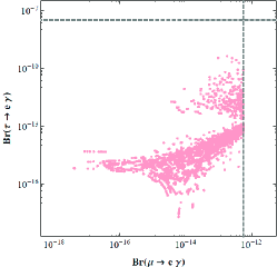
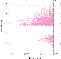
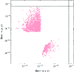
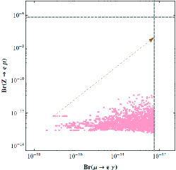
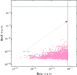
Figure 4: Correlations among the charged lepton flavor violating branching ratios for neutrino masses are of the inverted hierarchy. In these plots, $m_{\Delta}=1{\rm{TeV}}$, $m_{S}=7{\rm{TeV}}$ and $|(Y_{S})_{33}|=0.0097$. The dashed lines represent the current experimental limits at 90%C.L.

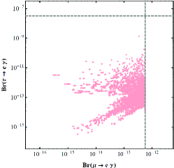
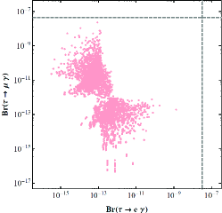
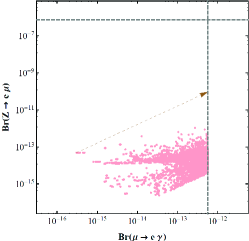
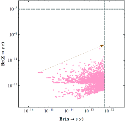
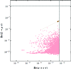
Figure 5: Correlations among the charged lepton flavor violating branching ratios for neutrino masses are of the normal hierarchy. In these plots, $m_{\Delta}=1{\rm{TeV}}$, $m_{S}=7{\rm{TeV}}$ and $|(Y_{S})_{33}|=0.0097$. The dashed lines represent the current experimental limits at 90%C.L.

All these plots have $|(Y_{S})_{33}|$ fixed at its maximally allowed value $0.0097$. From here, other configurations can be obtained by simply scaling down $Y_{S}$ by $Y_{S}\rightarrow\lambda^{-2}Y_{S}$ ( with $\lambda>1$ ). In response, all the LFV processes branching ratios move up as $\lambda^{4}$. In some plots, the dashed arrows are put in to guide the reader’s eyes and show the drifting direction of the branching ratios during the re-scaling. As the $Y_{S}$ is dialed down, all the points of ${\cal B}^{Z}_{ll^{\prime}}$ go up along the indicated direction until the $B(\mu\rightarrow e\gamma)$ hits the current experimental limit. Interestingly, we can predict the upper limits on ${\cal B}^{Z}_{ll^{\prime}}$, ranging from $10^{-11}$ to $10^{-9}$, for the $Y_{R}=0$ case. We stress that these upper limits are tied with the $Y_{R}=0$ assumption; they could be much larger if $Y_{R}\neq 0$. This part of parameter space of cZBM could be probed at the planned TeraZ collider where about $10^{12}$ Z bosons will be produced per year with a few $ab^{-1}$ luminosityTLEP ; CEPC . Moreover, this particular assumption will be ruled out if any excess was measured in the future experiment. On the other hand, the lower limits on these LFV processes are rather robust and insensitive to the $Y_{R}=0$ assumption. Similarly, interesting upper and lower bounds on ${\cal B}(\ell\rightarrow\ell^{\prime}\gamma)$ and the CP asymmetries $\eta_{\ell\ell^{\prime}}$ can be predicted in cZBM, see Tab.5. Note that the upper bounds on all three ${\cal B}(\ell\rightarrow\ell^{\prime}\gamma)$ are just below the current experimental limits. Any improvement in these measurements will cut across the interesting parameter space of cZBM. On the other hand, the cZBM with democratic $Y_{S}$ and $m_{\Delta}\sim{\cal O}({\rm{TeV}})$ can be falsified if no such cLFV processes had been detected above the predicted lower bounds in the future experiments.

	lower bounds	upper bounds (for $Y_{R}=0$)
$\mathcal{B}(\mu\rightarrow e\gamma)$	$3.05\times 10^{-16}$ ($3.98\times 10^{-18}$)	$5.7(5.7)\times 10^{-13}$
$\mathcal{B}(\tau\rightarrow e\gamma)$	$3.16\times 10^{-16}$ ($2.03\times 10^{-18}$)	$2.3(0.51)\times 10^{-9}$
$\mathcal{B}(\tau\rightarrow\mu\gamma)$	$4.67\times 10^{-17}$ ($1.68\times 10^{-16}$)	$3.4(2.8)\times 10^{-8}$
$\mathcal{B}^{Z}_{e\mu}$	$2.5\times 10^{-16}$ ($4.9\times 10^{-14}$)	$2.2(8.7)\times 10^{-11}$
$\mathcal{B}^{Z}_{e\tau}$	$2.9\times 10^{-16}$ ($4.6\times 10^{-14}$)	$3.6(1.0)\times 10^{-10}$
$\mathcal{B}^{Z}_{\mu\tau}$	$2.5\times 10^{-14}$ ($7.8\times 10^{-15}$)	$5.5(4.5)\times 10^{-9}$
$\eta_{\mu e}$	${}^{+.68}_{-.67}({}^{+2.1}_{-.97})\times 10^{-13}$	${}^{+2.6}_{-5.4}({}^{+9.3}_{-8.1})\times 10^{-13}$
$\eta_{\tau e}$	${}^{+2.4}_{-.20}({}^{+.20}_{-1.2})\times 10^{-12}$	${}^{+2.3}_{-.56}({}^{+.22}_{-.10})\times 10^{-11}$
$\eta_{\tau\mu}$	${}^{+2.3}_{-.78}({}^{+1.3}_{-1.3})\times 10^{-11}$	${}^{+3.7}_{-8.1}({}^{+3.0}_{-3.1})\times 10^{-11}$

Table 5: Range of $\mathcal{B}(\ell\to\ell^{\prime}\gamma)$, $\mathcal{B}(Z\rightarrow\ell\ell^{\prime})$, and $\eta_{\ell\ell^{\prime}}$ for $m_{\Delta}=1{\rm{TeV}}$ and $m_{S}=7{\rm{TeV}}$. The numbers( in the parentheses ) are for NH(IH) neutrino masses. The lower bounds are the lowest values found in the numerical search with $|(Y_{S})_{33}|=0.0097$. The upper bounds are found by rescaling $Y_{S}$, see text. Note that the sign for $\eta_{\ell\ell^{\prime}}$ could be either ways. For a different leptoquark/di-quark mass, all the values should be multiplied by a factor of $(1{\rm{TeV}}\cdot m_{S}/7m_{\Delta}^{2})^{2}$.

Note that the double ratio of any pair of cLFV process branching ratios is invariant under the $Y_{S}$ re-scaling and independent of $m_{\Delta}$. Our numerical also has concrete predictions for $Y_{R}=0$ and these double ratios depend on the neutrino mass pattern, see Fig.6. Therefore they could provide an intriguing mean to determine the neutrino mass hierarchy. In particular, the neutrino mass hierarchy can be unambiguously determined if the measured values fell into any of the decisive windows listed in Tab.6. Most of these interesting double ratio windows are plagued by either small cLFV branching ratios or very limited parameter space. However, $R_{5}\equiv{\cal B}(\tau\rightarrow\mu\gamma)/{\cal B}(\tau\rightarrow e\gamma)$ and $R_{7}\equiv{\cal B}^{Z}_{\mu\tau}/{\cal B}^{Z}_{\mu e}$ look quite promising. In the cZBM, if $R_{5}$ is measured in the future rare tau decay experiment to be within $0.03$ and $30$, the neutrino masses are of NH. If $R_{7}<1.0$ is measured in the future $Z$-factory, the neutrino masses are of IH in the cZBM. Even in the worst scenario that none of the measured double ratios overlap with these stated windows, one could still tell which neutrino mass hierarchy is more probable by simple statistics and probability theory. For example, if both $R_{4}$ and $R_{5}$ were measured to be $\sim 10^{3}$, then the IH is roughly 4 times more probable than the NH in the cZBM. The above discussion clearly demonstrates that the neutrino oscillation experiments and the cLFV measurements are complimentary to one another to better understand the origin of the neutrino masses.

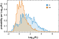
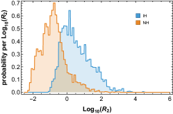
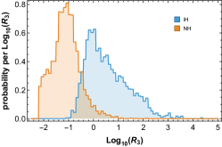
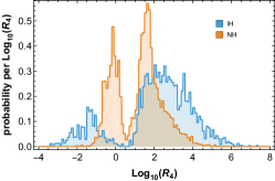
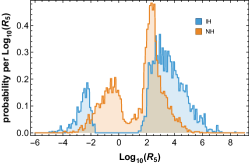
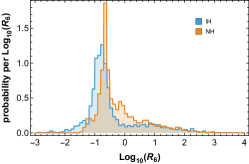
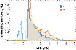
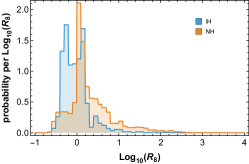
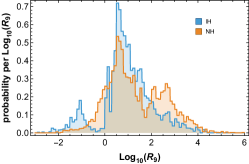
Figure 6: Side by side comparison of the double ratios in NH and IH. See Tab.6 for the double ratio definitions.

Double Ratio	IH	NH
$R_{1}\equiv{\cal B}^{Z}_{\mu\tau}/{\cal B}(\mu\rightarrow e\gamma)$	$R_{1}>10^{4}$ or $R_{1}<0.1$	N.A.
$R_{2}\equiv{\cal B}^{Z}_{e\tau}/{\cal B}(\mu\rightarrow e\gamma)$	$R_{2}>10^{3}$	$R_{2}<0.1$
$R_{3}\equiv{\cal B}^{Z}_{e\mu}/{\cal B}(\mu\rightarrow e\gamma)$	$R_{3}>10^{2}$	$R_{3}<0.1$
$R_{4}\equiv{\cal B}(\tau\rightarrow\mu\gamma)/{\cal B}(\mu\rightarrow e\gamma)$	$R_{4}>10^{6}$	$R_{4}<0.003$
$R_{5}\equiv{\cal B}(\tau\rightarrow\mu\gamma)/{\cal B}(\tau\rightarrow e\gamma)$	N.A.	$0.03<R_{5}<30$
$R_{6}\equiv{\cal B}(\tau\rightarrow e\gamma)/{\cal B}(\mu\rightarrow e\gamma)$	$R_{6}<0.03$	N.A.
$R_{7}\equiv{\cal B}^{Z}_{\mu\tau}/{\cal B}^{Z}_{\mu e}$	$R_{7}<1.0$	$R_{7}>3\times 10^{4}$
$R_{8}\equiv{\cal B}^{Z}_{e\tau}/{\cal B}^{Z}_{e\mu}$	N.A.	$R_{8}>10^{2}$
$R_{9}\equiv{\cal B}^{Z}_{\tau\mu}/{\cal B}^{Z}_{\tau e}$	$R_{9}<0.01$	$R_{9}>3\times 10^{4}$

Table 6: The definitions of the cLFV double ratios and the ranges which can be used to determine neutrino mass hierarchy.

5.2.2 Leptoquark decay branching ratios

First, some shorthand notations are introduced:

$$\Gamma^{\ell^{-}_{i}}_{\Delta}\equiv\sum_{j}\Gamma(\Delta\rightarrow\ell^{-}_{i}u_{j})\,,\Gamma^{\nu_{i}}_{\Delta}\equiv\sum_{j}\Gamma(\Delta\rightarrow\nu_{i}d_{j})\,,$$ (46)

where the quark flavors are summed over. For $Y_{R}=0$, the $SU(2)_{L}$ symmetry ensures that $\Gamma^{\ell^{-}_{i}}_{\Delta}=\Gamma^{\nu_{i}}_{\Delta}\propto|\sum_{j}(Y_{L})_{\ell_{i}j}|^{2}$. This corresponds to the $\beta=1/2$ case that 50% of the leptoquark decays into a neutrino and a down-type quark. Since the neutrino is hard to be tracked in the detector, we focus on the decay channels with a high energy charged lepton as the primordial final state and define

$$B^{\Delta}_{\ell_{i}}\equiv{\Gamma^{\ell^{-}_{i}}_{\Delta}\over\Gamma^{e^{-}}_{\Delta}+\Gamma^{\mu^{-}}_{\Delta}+\Gamma^{\tau^{-}}_{\Delta}}\,.$$ (47)

The above defined quantity is clearly independent of $m_{\Delta}$ and $Y_{S}$ re-scaling.

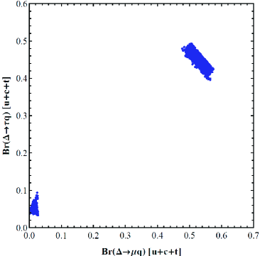
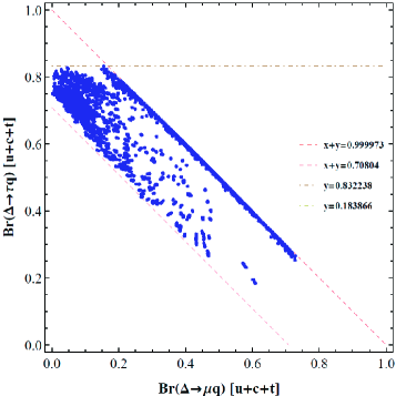
Figure 7: leptoquark decay branching ratios for (a) IH, (b) NH.

The decay branching ratios for leptoquark from our numerical study are displayed in Fig.7. It can be clearly seen in Fig.7 that, depending on the neutrino mass hierarchy, there are special patterns in the leptoquark decay branching ratios. Roughly speaking, for the IH case, the leptoquark decays are either (1) $B^{\Delta}_{e}\sim 1.0$ or (2) $B^{\Delta}_{\mu}\sim 55\%$ and $B^{\Delta}_{\tau}\sim 45\%$. On the other hand, for the NH case, the $B^{\Delta}_{\mu}$ and $B^{\Delta}_{\tau}$ are concentrated in the region roughly enclosed by $0.7\lesssim B^{\Delta}_{\mu}+B^{\Delta}_{\tau}\lesssim 1.0$ and $0.2\lesssim B^{\Delta}_{\tau}\lesssim 0.8$. In other words, $B^{\Delta}_{e}\lesssim 0.3$ if the neutrino masses are in the NH.

Surprisingly, our numerical study has not found any configuration which has either $B^{\Delta}_{\mu}\sim 100\%$ or $B^{\Delta}_{\tau}\sim 100\%$. Dictated by the neutrino oscillation data, the model predicts that the leptoquark can NOT decays purely into the 2nd or the 3rd generation charged leptons. These concrete branching ratios could be used to provide the new benchmark leptoquark mass limits with a better motivation.

6 Conclusion

We have studied the cZBM which exploits a scalar leptoquark $\Delta(3,1,-1/3)$ and a scalar di-quark $S(6,1,-2/3)$ to generate neutrino masses at the 2-loop level. The neutrino mass matrix element $M^{\nu}_{ij}$ ( i,j=1,2,3) is proportional to the product of $(Y_{L})_{ik}m^{d}_{k}(Y_{S}^{\dagger})_{kk^{\prime}}m^{d}_{k^{\prime}}(Y_{L}^{T})_{k^{\prime}j}$, see Eq.(2). The Yukawa couplings $Y_{L}$ and $Y_{S}$ are a priori unknown and arbitrary. To proceed, we have adopted a modest working assumption that all six $|Y_{S}|$ are of the same order. Then the $Y_{L}$ can be iteratively determined owing to the fact that $m_{\Delta},m_{S}\gg m_{b}\gg m_{s}\gg m_{d}$. Moreover, the mass of the lightest neutrino is of order $10^{-5}$ eV and the model disfavors the case of nearly degenerate neutrinos. The tree-level flavor violating processes will be inevitably mediated by $\Delta$ or $S$ with the realistic $Y_{L}$ which accommodates the neutrino data. Due to the different chiral structures, the contributions to the flavor violating processes from $Y_{L}$ and $Y_{R}$ do not interfere with each other at the tree-level. We have considered the case that $Y_{R}=0$ to minimized the tree-level flavor violating processes( and expect the same to happen for the loop induced cLFV). We also have argued that $Y_{R}=0$ is actually favored by the fact that there is no electron EDM has been observed yet. A comprehensive numerical study has been performed to look for the realistic $Y_{L}$ and $Y_{S}$ configurations which pass all the known experimental constraints on the flavor violating processes. The viable configurations were collected and have been used to calculate the resulting 1-loop charged lepton flavor violating $Z\rightarrow\overline{l}l^{\prime}$ and $l\rightarrow l^{\prime}\gamma$. Some of the realistic configurations could be probed in the forthcoming cLFV experiments. Interesting and robust lower bounds have been found for these cLFV, see Tab.5. Moreover, the neutrino mass hierarchy could be determined if the measured cLFV double ratio(s) is/are in some specific range(s), see Tab.6. For $Y_{R}=0$, $\Delta$ has $50\%$ of chance decaying into a charged lepton and an up-type quark. Specific ratios $\sum_{j}B(\Delta\rightarrow l_{i}u_{j})$ for each generation charged lepton $l_{i}$ have been predicted in this model. Given the potential link between the neutrino masses generation and $\Delta$, it seems well-motivated using the predicted leptoquark branching ratios as a benchmark scenario for the future scalar leptoquark search limits.

- (1) A. Zee, Nucl. Phys. B 264,99 (1986); K.S. Babu, Phys. Lett. B 203, 132 (1988).
- (2) S. Weinberg, Phys. Rev. Lett. 43, 1566 (1979).
- (3) P. Fileviez Perez and M. B. Wise, Phys. Rev. D 80, 053006 (2009) doi:10.1103/PhysRevD.80.053006 [arXiv:0906.2950 [hep-ph]].
- (4) H. Pas and E. Schumacher, Phys. Rev. D 92, no. 11, 114025 (2015) doi:10.1103/PhysRevD.92.114025 [arXiv:1510.08757 [hep-ph]].
- (5) W. Buchmuller, R. Ruckl and D. Wyler, Phys. Lett. B 191, 442 (1987) Erratum: [Phys. Lett. B 448, 320 (1999)].
- (6) S. Dimopoulos and L. Susskind, Nucl. Phys. B 155, 237 (1979).
- (7) S. Dimopoulos, Nucl. Phys. B 168, 69 (1980).
- (8) E. Eichten and K. D. Lane, Phys. Lett. B 90, 125 (1980).
- (9) V. D. Angelopoulos, J. R. Ellis, H. Kowalski, D. V. Nanopoulos, N. D. Tracas and F. Zwirner, Nucl. Phys. B 292, 59 (1987).
- (10) J. L. Hewett and T. G. Rizzo, Phys. Rept. 183, 193 (1989).
- (11) The CMS Collaboration, CMS PAS EXO-12-041 (2014/07/10).
- (12) The CMS Collaboration, CMS PAS EXO-12-042 (2013/05/30).
- (13) The CMS Collaboration, CMS PAS EXO-13-010 (2014/07/05)
- (14) The ATLAS Collaboration, Phys. Lett. B 709 (2012) 158.
- (15) The ATLAS Collaboration, Eur. Phys. J. C (2012) 72:2151.
- (16) The ATLAS Collaboration, JHEP06(2013)033.
- (17) Francesco Romeo, ATLAS and CMS collaborations, CMS CR-2014-241
- (18) The ZEUS Collaboration, Phys. Rev. D 86(2012)012005; 1205.5179[hep-ex].
- (19) V. Khachatryan et al. [CMS Collaboration], Phys. Rev. Lett. 116, no. 7, 071801 (2016)
- (20) M. Carpentier and S. Davidson, Eur. Phys. J. C 70 (2010) 1071-1090; arXiv: 1008.0280v2 [hep-ph].
- (21) M. Kohda, H. Sugiyama, K. Tsumura, Phys. Lett. B 718 (2013) 1436; arXiv: 1210.5622[hep-ph].
- (22) F. S. Queiroz, K. Sinha and A. Strumia, Phys. Rev. D 91, no. 3, 035006 (2015) doi:10.1103/PhysRevD.91.035006 [arXiv:1409.6301 [hep-ph]].
- (23) W. F. Chang, J. N. Ng and J. M. S. Wu, Phys. Rev. D 78, 096003 (2008) doi:10.1103/PhysRevD.78.096003 [arXiv:0806.0667 [hep-ph]]; W. F. Chang, J. N. Ng and J. M. S. Wu, Phys. Rev. D 79, 056007 (2009) doi:10.1103/PhysRevD.79.056007 [arXiv:0809.1390 [hep-ph]].
- (24) W. F. Chang, I. T. Chen and S. C. Liou, Phys. Rev. D 83, 025017 (2011) doi:10.1103/PhysRevD.83.025017 [arXiv:1008.5095 [hep-ph]].
- (25) K.S. Babu and C. Macesanu, Phys. Rev. D 67, 073010 (2003); D. A. Sierra and M. Hirsch, JHEP 12 2006, 052; M. Nebot, J. F. Oliver, D. Palao and A. Santamaria, Phys. Rev. D 77, 093013 (2008).
- (26) K.L. McDonald and B.H.J. Mckellar, arXiv: hep-ph/0309270.
- (27) J. M. Arnold, B. Fornal and M. B. Wise, Phys. Rev. D 88, 035009 (2013) doi:10.1103/PhysRevD.88.035009 [arXiv:1304.6119 [hep-ph]].
- (28) We-Fu Chang, John N. Ng, Jackson M. S. Wu, Phys. Rev. D 86(2012)033003; arXiv: 1206.5047 [hep-ph];
- (29) W.-F. Chang, W.-P. Pan, F. Xu, Phys. Rev. D 88(2013)033004; arXiv:1303.7035 [hep-ph].
- (30) C.-S. Chen, C.-Q. Geng, D. Huang, L.-H. Tsai, arXiv: 1301:4694[hep-ph].
- (31) G. Aad et al. [ATLAS Collaboration], Phys. Rev. D 90, 112015 (2014).
- (32) ATLAS Collaboration, Phys. Lett. B732 (2014) 8.
- (33) The CMS Collaboration, Eur. Phys. J. C (2014) 74:3076.
- (34) CMS Collaboration, Phys. Lett. B726 (2013) 587
- (35) K.A. Olive et al. [Particle Data Group], Chin. Phys. C, 38, 090001 (2014).
- (36) P.A.R. Ade et al. [Planck collaboration], arXiv: 1502.01589v2 [astro-ph.CO].
- (37) S. M. Bilenky and C. Giunti, Mod. Phys. Lett. A 27, 1230015 (2012).
- (38) M. Bona, et. al. [UTfit Collaboration], JHEP03 (2008) 049.
- (39) Y. Kuno and Y. Okada, Rev. Mod. Phys. 73, 151 (2001);
- (40) W.-F. Chang, J.N. Ng, Phys. Rev. D 71, 053003 (2005).
- (41) G.W. Bennett et al. [Muon (g-2) Collaboration], Phys. Rev. D 73, 072003 (2006).
- (42) G. F. Giudice, P. Paradisi, and M. Passera, J. High Energy Phys. 11 (2012) 113.
- (43) The ACME Collaboration, Science343, 269(2014).
- (44) G. Aad et al., the ATLAS Collaboration, Phys. Rev. D 90, 072010 (2014).
- (45) J. Bernabeu, M. B. Gavela and A. Santamaria, Phys. Rev. Lett. 57, 1514 (1986). doi:10.1103/PhysRevLett.57.1514
- (46) N. Rius and J. W. F. Valle, Phys. Lett. B 246, 249 (1990). doi:10.1016/0370-2693(90)91341-8
- (47) J. Adam et. al., [MEG Collaboration], Phys. Rev. Lett. 110, 201801 (2013).
- (48) B. Aubert et. al. [BaBar Collaboration], Phys. Rev. Lett. 104, 021802 (2010).
- (49) A. M. Baldini et al. [MEG Collaboration], Eur. Phys. J. C 76, no. 8, 434 (2016) doi:10.1140/epjc/s10052-016-4271-x [arXiv:1605.05081 [hep-ex]].
- (50) M. Bicer et al. [TLEP Design Study Working Group Collaboration], JHEP 1401, 164 (2014) doi:10.1007/JHEP01(2014)164 [arXiv:1308.6176 [hep-ex]].
- (51) CEPC-SPPC Study Group, IHEP-CEPC-DR-2015-01, IHEP-TH-2015-01, HEP-EP-2015-01.