The Distant Outer Gas Arm Between $35^{\circ}$ and $45^{\circ}$

Abstract

The Galactic plane has been mapped from $l=$34$\fdg$75 to 45$\fdg$25 and $b=-$5$\fdg$25 to 5$\fdg$25 in the CO ($J$=1–0) emission with the 13.7 m telescope of the Purple Mountain Observatory. The unbiased survey covers a large area of 110 square degrees sampled every 30^′′ with a velocity resolution of $\sim 0.2\,{\rm km}\,{\rm s}^{-1}$. In this paper, we present the result of an unbiased CO survey of this longitude and latitude range in the velocity range from $-60$ to $-10\,{\rm km}\,{\rm s}^{-1}$. Over 500 molecular clouds (MCs) are picked out from the ¹²CO ($J$=1–0) emission, and 131 of these MCs are associated with ¹³CO emission. The distant MCs, which lie beyond the solar circle and are mostly concentrated in the Galactic plane, trace the large-scale molecular gas structure over 10 degrees of Galactic azimuth. We find that the distribution of the distant MCs can be well fitted by a Gaussian function with a full width at half maximum (FWHM) of 0$\fdg$7 with the Galactic latitude. We suggest that the CO emission of the segment is from the Outer Arm. The physical mid-plane traced by the Outer Arm seems to be slightly displaced from the IAU-defined plane on a large scale, which could be explained by the warped plane at large Galactocentric distances of  $>$$\sim$ 10 kpc and the apparent tilted mid-plane to the projected IAU-defined plane caused by the Sun’s $z$-height above the disk for distances near and within the Solar circle. After removing the effect of the warp and tilted structure, the scale height of the MCs in the Outer Arm is about 0$\fdg$6 or 160 pc at a heliocentric distance of 15 kpc. If the inner plane of our Galaxy is flat, we can derive an upper limit of the Sun’s offset of $\sim$17.1 pc above the physical mid-plane of the Milky Way. We also discuss the correlations between the physical parameters of the distant MCs, which is quite consistent with the result of other studies of this parameter.

1. INTRODUCTION

Molecular clouds (MCs), as observed in CO surveys of the Galactic plane, play an important role in studying star formation and the structure of the Galaxy (e.g., Clemens, 1985; Dame et al., 1987, 2001; Heyer & Terebey, 1998; Jackson et al., 2006; Burton et al., 2013). Several works were concentrated on the large-scale structure traced by MCs in the first Galactic quadrant (e.g., Dame & Thaddeus, 1985; Clemens et al., 1986, 1988; Dame et al., 1986; Scoville et al., 1987; Jacq et al., 1988; Solomon & Rivolo, 1989; Roman-Duval et al., 2010). However, the CO emission lying beyond the solar circle in the first quadrant of the Galaxy is less studied (e.g., Section 3.1.5 and Figure 3 in Dame et al., 2001). The only cases are the study of the MCs in the Outer Arm of the Galaxy for the region of $l>55^{\circ}$ in the first quadrant (using the NRAO 11 m telescope, Kutner & Mead, 1981; Mead & Kutner, 1988) and for the region between $l=65^{\circ}$ and $71^{\circ}$ (using the CfA 1.2 m and the Bell 7 m telescopes, Digel et al., 1990).

The Milky Way Imaging Scroll Painting (MWISP) project is a high resolution ($50^{\prime\prime}$) ¹²CO ($J$=1–0), ¹³CO ($J$=1–0), and C¹⁸O ($J$=1–0) survey of the northern Galactic plane, performed with the Purple Mountain Observatory Delingha 13.7 m telescope. The survey started in 2011, and will cover Galactic longitudes from $l=-10^{\circ}$ to $250^{\circ}$ and latitudes from $b=-5^{\circ}$ to $5^{\circ}$ over a period of $\sim$10 years. The Galactic plane will be covered by full-sampling observations with the spectral line On-The-Fly (OTF) mode. The survey has equal sensitivity over all regions of the sky mapped and thus it is unbiased. One of the goals of this project is to study the physical properties of MCs along the northern Galactic plane. As of this writing the survey has completed about half of its planned area of coverage.

Benefiting from the large unbiased survey of the MWISP, we can systematically investigate the characteristics of the structure of the Galaxy using the molecular gas. Recently, a CO spiral arm lying beyond the Outer Arm in the first Galactic quadrant was identified by Dame & Thaddeus (2011) using the CfA 1.2 m telescope. Based on our new CO data of the MWISP, the extension of the above arm, which is probably the Scutum-Centaurus Arm into the outer second quadrant, has been revealed very recently by Sun et al. (2015).

In this paper, we investigate the Outer Arm (the Norma-Cygnus Arm, e.g., see the recent review in Vallée, 2014) in the first quadrant of the Galaxy according to the distribution of the CO gas between $l=35^{\circ}$ to $45^{\circ}$. The distant MCs beyond the solar circle traced by CO emission have a negative velocity in the direction that we are interested in. The velocity range of the CO gas within the arm is about $-60$ to $-10\,{\rm km}\,{\rm s}^{-1}$ in the direction (Section 3.3). The Outer Arm lies beyond the solar circle in the Galactic longitude range of $l\mbox{\hskip 1.99997pt\raisebox{2.15277pt}{$>$}\raisebox{-2.15277pt}{$\sim$}\hskip 1.99997pt}30^{\circ}$ in the first quadrant of the Milky Way, thus the molecular gas traced by CO emission does not suffer the kinematic distance ambiguity encountered in the region within the Solar circle. Generally speaking, in this quadrant, the more negative the value of the velocity is, the larger the distance of the MC. Moreover, the large sample of the distant MCs provides a good opportunity to study the global cloud parameters (Section 3.6) since the data have a high signal-to-noise ratio and there is little overlap between the clouds (Section 3.1).

We present observations and data reductions of the survey in Section 2. In Section 3.1 and 3.2, we describe the MCs identification and the distribution of the distant MCs, respectively. We find that the physical mid-plane traced by the distant CO gas is slightly displaced from the IAU-defined plane of $b=0^{\circ}$ (Section 3.3). We also discuss the relationship between the two planes in Section 3.4. In Section 3.5, we derive the Sun’s offset above the physical mid-plane because of the apparent displacement between the two planes for regions near and within the solar circle. The statistical properties of the distant MCs are discussed in Section 3.6. Finally, the summary is given in Section 4.

2. CO OBSERVATIONS AND DATA REDUCTIONS

We mapped $\sim$110 square degrees (439 cells) in the region between Galactic longitudes 34$\fdg$75–45$\fdg$25 and latitudes $-$5$\fdg$25 to 5$\fdg$25 during 2011 November to 2015 March using the 13.7 m millimeter-wavelength telescope located at Delingha in China. The nine-beam Superconducting Spectroscopic Array Receiver (SSAR) system was used at the front end and each Fast Fourier transform spectrometer (FFTS) with a bandwidth of 1 GHz provides 16,384 channels and a spectral resolution of 61 kHz (see the details in Shan et al., 2012). The molecular lines of ¹²CO ($J$=1–0), ¹³CO ($J$=1–0) and C¹⁸O ($J$=1–0) were observed simultaneously with the OTF method. Each cell with dimension 30${}^{\prime}\times 30^{\prime}$ was scanned at least in two orthogonal directions, along the Galactic longitude and the Galactic latitude, in order to reduce the fluctuation of noise. The half-power beamwidth (HPBW) of the telescope was about $50^{\prime\prime}$ at a local oscillating frequency of 112.6 GHz and the pointing accuracy was better than $5^{\prime\prime}$ in all observing epochs.

All cells were reduced using the GILDAS/CLASS package. After removing the bad channels in the spectra and correcting the first order (linear) baseline fitting, the antenna temperature ($T_{\rm A}^{\star}$) was converted to the main beam temperature ($T_{\rm mb}$) with the relation $T_{\rm mb}=T_{\rm A}^{\star}/(f_{\rm b}\times\eta_{\rm mb})$. In the above conversion, the beam-filling factor of $f_{\rm b}$ is assumed to be one and the beam efficiency $\eta_{\rm mb}$ is from the status report of the 13.7 m telescope of the Purple Mountain Observatory. The typical sensitivity (rms) is about 0.5 K for ¹²CO ($J$=1–0) at the channel width of 0.16$\,{\rm km}\,{\rm s}^{-1}$ and 0.3 K for ¹³CO ($J$=1–0) and C¹⁸O ($J$=1–0) at 0.17$\,{\rm km}\,{\rm s}^{-1}$ with a spatial resolution of $<1^{\prime}$.

Finally, all spectra of CO in each cell were converted to the three-dimensional (3D) cube mosaic data together with a grid spacing of $30^{\prime\prime}$ and the channel width of 0.16$\,{\rm km}\,{\rm s}^{-1}$ for ¹²CO ($J$=1–0) and 0.17$\,{\rm km}\,{\rm s}^{-1}$ for ¹³CO ($J$=1–0) and C¹⁸O ($J$=1–0) for subsequent analysis.

3. RESULTS AND DISCUSSION

3.1. MCs Identification

We carefully checked the 3D cube data channel by channel before investigating the characters of the MCs that we are interested in. We find that the distant MCs in the velocity interval of $-60$ to $-10\,{\rm km}\,{\rm s}^{-1}$ are isolated in the $l$–$b$–$v$ space. That is, most of them show the distinct structure in the space of $l$–$b$ and there is, therefore, little overlapping in the velocity axis over the large survey’s area. Moreover, it is not surprising that their ¹²CO ($J$=1–0) emission is stronger than that of the ¹³CO ($J$=1–0). No $>3\times$rms C¹⁸O ($J$=1–0) emission ($T_{\rm peak18}$) is detected in the whole region in the velocity range. Only insignificant C¹⁸O emission ($T_{\rm peak18}\sim 2\times$rms) can be found toward the MCs’ region with some detectable ¹³CO emission (e.g., $T_{\rm peak13}>5\times$rms). We do not discuss these weak C¹⁸O emission features in this paper.

According to the discrete feature of the distant MCs, we used the FINDCLUMPS tool in the CUPID package (part of the STARLINK package) to identify MCs in the ¹²CO and ¹³CO FITS cube. The CLUMPFIND algorithm (Williams et al., 1994) is applied in the process of identification. We set the parameter Tlow=3$\times$rms for ¹²CO and Tlow=2.7$\times$rms for ¹³CO, which determines the lowest level to contour an MC, in order to obtain as much of the emission as possible and to avoid the contamination of the noise based on our large survey data. The parameter of DeltaT=9$\times$rms, which shows the contour increment, is large since we do not care about the properties of the structure of the bright parts embedded in the extended MCs. Other input parameters of the CLUMPFIND algorithm are typical to identify those distant MCs for the 3D cube data. Considering the irregular shape of the MCs, we use a polygon to describe the MC’s boundary in the $l$–$b$ space. Some objects are rejected if their sizes are less than the criteria: FwhmBeam=1.5 pixel, VeloRes=2 channel, and MinPix=16.

It is worthwhile to note that sometimes an individual MC is decomposed to several MCs because of the small velocity separation of $\sim 1-2\,{\rm km}\,{\rm s}^{-1}$ within roughly the same $l$–$b$ region. However, the above case is a rare population compared to that of all detected MCs (Figures 1 and 2). On the other hand, some point-like sources ( $<$$\sim$  3–4 pixels) cannot be picked out because of their smaller sizes. Some faint diffuse structures where ¹²CO ($J$=1–0) emission is near the noise level of the survey cannot be identified due to their poor signal-to-noise ratio. Further observations are needed to confirm these MCs with small size or faint emission.

Finally, we identified 575 and 131 MCs from the ¹²CO and ¹³CO emission based on the CLUMPFIND algorithm, respectively. The parameters of each MC, such as position, LSR velocity, one-dimensional velocity dispersion, the peak value, the size, and the luminosity, were obtained directly from the automated detection routine. The parameters of the resolved MCs are summarized in Tables 1 and 2: (1) the ID of the identified MCs, arranged from the low Galactic longitude; (2) and (3) the MCs’ Galactic coordinates ($l$ and $b$); (4) the MCs’ LSR velocity ($V_{\rm LSR}$); (5) the MCs’ full width at half maximum (FWHM, $\Delta V_{\rm FWHM}$), defined as 2.355 times of the velocity dispersion $\sigma_{v}$ for a Gaussian line; (6) the MCs’ peak emission ($T_{\rm peak}$); (7) the MCs’ area; (8) the MCs’ integrated intensity ($W_{\rm CO}$) within a defined area; (9) the MCs’ total luminosity ($L_{\rm CO}=W_{\rm CO}\times\rm{Area}$). Finally, we use MWISP Glll.lll$\pm$bb.bbb to name an MC detected from the survey data.

We made the integrated intensity map of the ¹²CO ($J$=1–0) emission in the velocity interval of $-1.6\times l$+$13.2\,{\rm km}\,{\rm s}^{-1}$ to $-10\,{\rm km}\,{\rm s}^{-1}$ (Section 3.3) in Figure 1. After overlapping the 575 resolved MCs on the map, we find that the distribution of the CO gas is well traced by the result from the automated cloud-finding routine. It shows that the CLUMPFIND algorithm is thus reliable to pick out the distant MCs. In addition, the sample of the MCs can be used to investigate the large structures of the spiral arm (Section 3.3) and the properties of the distant MCs (Section 3.6).

Figure 2 displays the intensity-weighted velocity (the first moment) map of the ¹²CO ($J$=1–0) emission. The distribution of the 131 ¹³CO MCs is also consistent with that of the bright ¹²CO ($J$=1–0) emission. The blue stripes at $l=$41$\fdg$5 and $b=-$1$\fdg$5 are from the bad channels, which show regular oscillation along the velocity axis with intensity of $-2$ to 3 K. The abnormal feature can be easily distinguished from the CO emission of MCs.

We also present the typical spectra of four resolved MCs (¹²CO with the black line and ¹³CO$\times 2$ with blue) in Figure 3. All spectra in Figure 3 show good baselines. The CO emission of the MCs can be easily discerned from the spectra and the peak of ¹³CO ($J$=1–0) emission is roughly corresponding to that of the ¹²CO ($J$=1–0) line (Figure 3).

3.2. Spatial Distribution of the Distant Molecular Gas

We show the 575 MCs in the Galactic coordinate system in Figure 4, in which the filled circle indicates the position and the size (scaled with CO luminosity) of MCs and the color indicates the LSR velocity of MCs. All identified MCs are in the region of the Galactic latitude $b=-$1$\fdg$8 to $b=$2$\fdg$2, which indicates that the molecular gas is roughly concentrated in and around the Galactic plane (mainly in the region of $b\sim-$0$\fdg$5 to 1$\fdg$5). The map also shows that the distribution of the MCs is not uniform with Galactic longitude.

Figure 5 is the normalized histogram of the MCs with the Galactic longitude (left panel) and the Galactic latitude (right panel). According to the left panel of Figure 5, we find that the spatial distribution of the MCs is not uniform again. Several distribution peaks of the MCs are clearly discerned at $l=$35$\fdg$25, 39^∘, 42^∘, and 44^∘, respectively. The concentrated groups of these MCs can also be seen in the same region of Figure 4. The map in the right panel of Figure 5 shows that the MCs are mainly located within a limited range of the Galactic latitude, which indicates that the molecular gas in the velocity interval is actually from the Galactic plane with a distribution peak of $b=$0$\fdg$42.

We also made the position$-$velocity (PV) map of the MCs along the Galactic longitude (Figure 6), in which the distribution of the MCs is similar to that in Figure 5. The velocity gradient of the MCs can be seen on a large scale (see green dashed line in Figure 6), which shows the velocity trend of the Outer Arm along the Galactic longitude (Section 3.3). The distribution of the MCs in the longitude$-$velocity diagram seems to display some asymmetrical ripples, which is a feature that is probably from the substructures of the Outer Arm in this direction.

We note that some MCs are concentrated within groups. These MC groups seem to display partial shell structures, which probably relate to the star forming activity within the Outer Arm. We searched for the MCs associated with the massive star formation regions based on our unbiased CO survey. The information of the associations is listed in Table 3. We find that the distribution of the massive star-forming regions in the Outer Arm, which are mainly located at $l=39^{\circ}$, $42^{\circ}$, and $44^{\circ}$, is associated with that of the CO peaks in the $l$–$b$ space (see the 21 H ii regions marked with black circles and five 6.7 GHz masers marked with black triangles in Figure 2). This result shows that star formation activity is very common in the distant MCs of the Outer Arm. We will study the interesting structures and the massive star-forming activities in the future.

3.3. Outer Gas Arm Traced by CO emission

In the direction of $l=35^{\circ}$ to $45^{\circ}$, we note that the Outer Arm LSR velocity locates between the Perseus Arm and the Scutum-Centaurus Arm. That is, the Perseus Arm, the Outer Arm, and the Scutum-Centaurus Arm are encountered in this direction, each with different and decreased LSR velocity (see Figures 9 and 10 in Reid et al., 2016). Part of the molecular gas’ emission in the velocity interval of 0 to $-10\,{\rm km}\,{\rm s}^{-1}$ is from the Perseus Arm. The molecular gas of the Local Arm (Xu et al., 2013) probably also contributes to some emission in the velocity range of 0 to $-10\,{\rm km}\,{\rm s}^{-1}$. And the molecular gas with the LSR velocity $<-1.6\times l$+$13.2\,{\rm km}\,{\rm s}^{-1}$ is probably from a segment of a spiral arm at Galactocentric radii of R${}_{\rm GC}\sim$13–14 kpc (the value of -1.6 $\,{\rm km}\,{\rm s}^{-1}$Degree^-1 is from Dame & Thaddeus, 2011). In order to isolate the emission from the three spiral arms, we use the molecular gas in the velocity cutoff of $-1.6\times l$+$13.2\,{\rm km}\,{\rm s}^{-1}$ to $-10\,{\rm km}\,{\rm s}^{-1}$ to trace the Outer Arm (see the yellow dashed lines in Figure 6). Actually, the large-scale segment of the Outer Arm can be discerned from the longitude$-$velocity diagram of CO emission, in which the CO emission of the Outer Arm’s MCs is mainly in the above velocity range and their distribution can be described as $V_{\rm LSR}=-2.78\times l+75.9\,{\rm km}\,{\rm s}^{-1}$ (see the green dashed line in Figure 6) based on ¹³CO emission (excluding MCs near $l\sim 44^{\circ}$ and $V_{\rm LSR}\sim-20\,{\rm km}\,{\rm s}^{-1}$).

We use a Gaussian function, $f(b)\sim e^{-\frac{(b-b_{0})^{2}}{2\sigma^{2}}}$, to fit the distribution of the MCs with the Galactic latitude (the right panel in Figure 5). The dashed blue line shows the best fit: $b_{0}$=0$\fdg$42 and $\sigma$=0$\fdg$29. It indicates that the distant MCs in the velocity interval are mainly distributed within a narrow range of the Galactic latitudes of FWHM=2.355$\sigma\sim$0$\fdg$7. We thus suggest that the large amount of the CO emission actually traces the Outer Arm of the Milky Way.

The best Gaussian fit also shows that the distribution peak of the MCs in the segment is not around $b=0^{\circ}$ but $b$=0$\fdg$42, which probably indicates that the Outer Arm traced by the molecular gas is slightly displaced with respect to the IAU-defined plane (see the details in Section 3.4). We also use a linear relation, $b$=0$\fdg$0377$\times l-$1$\fdg$0893 (the thick blue line in Figure 4), to describe the distribution of the MCs in the $l$–$b$ space. The fitted blue line represents the physical mid-plane with respect to the IAU-defined plane of $b=0^{\circ}$. It indicates that the Outer Arm traced by the CO gas passes through the IAU-defined plane of $b=0^{\circ}$ at $l=$28$\fdg$9. The molecular gas of the Outer Arm in the range of $l\mbox{\hskip 1.99997pt\raisebox{2.15277pt}{$<$}\raisebox{-2.15277pt}{$\sim$}\hskip 1.99997pt}$28$\fdg$9 is mostly within the solar circle and the distribution of the MCs with latitude is mainly $b<0^{\circ}$ (see the Norma-Cygnus arm in Figure 3 of Vallée, 2014). The longitude$-$velocity relation from Figure 6 also indicates that the LSR velocity of the Outer Arm is roughly $\mbox{\hskip 1.99997pt\raisebox{2.15277pt}{$>$}\raisebox{-2.15277pt}{$\sim$}\hskip 1.99997pt}0\,{\rm km}\,{\rm s}^{-1}$ at $l\mbox{\hskip 1.99997pt\raisebox{2.15277pt}{$<$}\raisebox{-2.15277pt}{$\sim$}\hskip 1.99997pt}$28$\fdg$9. The feature is probably related to the Sun’s offset from the physical mid-plane (see Sections 3.4 and 3.5).

Using the 21 cm H i data from the VLA Galactic plane survey (VGPS; Stil et al., 2006), Dame & Thaddeus (2011) found that the Outer Arm traced by the H i gas is mainly below the plane of $b=0^{\circ}$ in the region of $l=25^{\circ}-30^{\circ}$ (see Figure 2 in their paper). In other words, at $l<30^{\circ}$ the Outer Arm seems to be below the IAU-defined plane in the first Galactic quadrant. According to our linear fit of the CO emission, in the region of $l=25^{\circ}-30^{\circ}$ the Galactic latitude distribution of the Outer Arm should peak at $b\sim-$0$\fdg$1, which is roughly consistent with the result of H i gas (see Figure 2 in Dame & Thaddeus, 2011).

Based on the Galactic parameters of Model A5 of Reid et al. (2014), we suggest that the heliocentric distance of the 10^∘ segment of the Outer Arm is about 15.1–15.6 kpc, which is a value that is quite consistent with the result of other models (e.g., McClure-Griffiths & Dickey, 2007; Foster & Cooper, 2010). The Galactocentric radii of the arm, R_GC, in the direction is about 9.5–11.4 kpc accordingly. After subtracting the effect of the tilted structure with the Galactic longitude (the thick blue line in Figure 4), we derived that the scale height of the MCs in the Outer Arm is about 0$\fdg$6 (or $\sim$160 pc at a heliocentric distance of 15 kpc). It is roughly consistent with the FWHM of the molecular disk of the Milky Way in such Galactocentric radii (see Table 1 and Figure 3 in Nakanishi & Sofue, 2006).

The total ¹²CO luminosity of the segment of the spiral arm is about 2.1$\times 10^{5}$ K$\,{\rm km}\,{\rm s}^{-1}$pc² at a heliocentric distance of 15 kpc. Therefore, the total molecular gas within the segment is about 9$\times 10^{5}M_{\odot}$ by adopting the mean CO-to-H₂ mass conversion factor $X_{\rm CO}$=$2\times 10^{20}$ cm^-2K^-1km^-1s (Bolatto et al., 2013) and a mean molecular weight per H₂ molecule of 2.76. We mention that the total mass of the segment estimated above is probably the lower limit because some weak ¹²CO emission is not accounted for in Table 1 (Section 3.1) and the value of $X_{\rm CO}$ is probably underestimated for the outer Milky Way (Bolatto et al., 2013).

Based on Table 1, the ¹²CO luminosity of the segment of the spiral arm is about 2.1$\times 10^{5}$ K$\,{\rm km}\,{\rm s}^{-1}$pc² at a heliocentric distance of 15 kpc. The molecular gas within the segment is about 0.9$\times 10^{6}M_{\odot}$ by adopting the mean CO-to-H₂ mass conversion factor $X_{\rm CO}$=$2\times 10^{20}$ cm^-2K^-1km^-1s (Bolatto et al., 2013) and a mean molecular weight per H₂ molecule of 2.76. For comparison, the total ¹²CO luminosity of the segment of $\sim 2.6\times 10^{4}$ K$\,{\rm km}\,{\rm s}^{-1}$arcmin² can be obtained by integrating velocity channels from $-1.6\times l$+$13.2\,{\rm km}\,{\rm s}^{-1}$ to $-10\,{\rm km}\,{\rm s}^{-1}$ for the covered map. Therefore, our estimate for the total molecular mass of the segment of the Outer Arm is 2.2$\times 10^{6}M_{\odot}$. The result indicates that over half of the total mass appears to be missed due to the relatively high criterion of Tlow=3$\times$rms in the CLUMPFIND method. The difference between the above estimations probably indicates that about 60% of the molecular gas probably resides within small, cold, and$\//$or faint, diffuse clouds that cannot be included in our catalog (see also, e.g., Section 5.1.3 of Heyer & Dame, 2015). We mention that the total mass of the segment estimated above is probably the lower limit because some weak ¹²CO emission is not accounted for and the value of $X_{\rm CO}$ is probably underestimated for the outer Milky Way (Bolatto et al., 2013). Assuming a constant value of $X_{\rm CO}$= $2\times 10^{20}$ cm^-2K^-1km^-1s and a heliocentric distance of 15 kpc, the mass surface density of the distant MCs is about $22M_{\odot}$ pc^-2, which is roughly consistent with the character of MCs in the outer Galaxy (see, e.g., Figure 8 in Heyer & Dame, 2015).

3.4. Physical Mid-plane Traced by the Outer Arm

In this section, we investigate the relationship between the physical mid-plane and the IAU-defined plane of $b=0^{\circ}$ in the view of the molecular gas on a large scale based on the new CO survey.

Generally, warps are common in spiral disks of galaxies (e.g. Reshetnikov & Combes, 1998; Schwarzkopf & Dettmar, 2001; Reshetnikov et al., 2002). For example, NGC 4013 shows a prodigious warp in its outer parts, in which the gas layer curves away from the plane of the inner disk (Bottema, 1996). In the Milky Way, the Hi layer was also found to be warped from the Solar radius outwards (e.g., Burke, 1957; Oort et al., 1958; Henderson et al., 1982). Furthermore, the stellar warp of the Milky Way is similar to the gaseous warp, but smaller in amplitude (e.g., Freudenreich et al., 1994; Freudenreich, 1998; Drimmel & Spergel, 2001).

On the other hand, the inner disk of the Milky Way is probably observed to be tilting because of the offset of the Sun (Hammersley et al., 1995). That is, the physical mid-plane projected on the sky displays an apparent change in latitude with respect to longitude across some regions of the sky. Previously, astronomers often used the star-counts method to derive the position of the Sun (e.g., Hammersley et al., 1995; Humphreys & Larsen, 1995; Chen et al., 2001; Maíz-Apellániz, 2001; Joshi, 2007; Majaess et al., 2009). These studies found that the Sun’s vertical displacement from the physical mid-plane is $\sim$10–30 pc (refer to Table 1 in Reed, 2006). By studying the infrared dark cloud (IRDC) “Nessie,” Goodman et al. (2014) recently suggested that the very long and dense filamentary IRDC represents a spine-like bone of the major spiral arm, the Scutum-Centaurus Arm, in the fourth quadrant of the Milky Way. They also suggested that the latitude of the true Galactic mid-plane traced by the spiral arm is $b\sim-$0$\fdg$4 (but not $b=0^{\circ}$) because of the Sun’s height off of the physical mid-plane of the Milky Way (see Figure 2 and Section 3.1 in Goodman et al., 2014).

Here we discuss the Galactic structure traced by CO emission of the Outer Arm. Both of the effects of the warp and the tilted plane (because of the Sun’s offset from the physical mid-plane) were considered. We explored three typical models for comparison with our observations: the gaseous warp model from the Galactic Hi data ($m=1$ mode for a cutoff at R_GC=10 kpc, Levine et al., 2006); the stellar warp model from 2MASS data (a $\gamma_{\rm warp}$ of 0.09 and a cutoff at R_GC=8.4 kpc, Reylé et al., 2009); and the tilted-plane model for the inner Galaxy (R${}_{\rm GC}<7$ kpc, and see Equation 5 in Hammersley et al., 1995). The $\gamma_{\rm warp}$ in the stellar warp model is defined as the ratio between the displacement (z_mid-plane) of the physical mid-plane from the IAU-defined plane of $b=0^{\circ}$ and the Galactocentric radii of R_GC (refer to Section 2.3 and Figure 9 in Reylé et al., 2009). For two warp models, we assume that the Sun roughly lies on the line of nodes of the warp (i.e., $\phi_{\rm warp}=0^{\circ}$, Burton, 1988; Binney & Merrifield, 1998). Based on the best fit of the longitude$-$velocity diagram ($V_{\rm LSR}=-2.78\times l+75.9\,{\rm km}\,{\rm s}^{-1}$; Figure 6), we can kinematically calculate the Galactocentric radii and the height of the physical mid-plane traced by the Outer Arm using the A5 rotation curve model of Reid et al. (2014). Thus, when the R_GC–z_mid-plane relation is obtained, we can directly compare the slope and the amplitude of the different models (the dotted lines) with those of the observations (the blue line) in the $l-b$ map (Figure 4). Here, the slope is defined as the ratio between z_mid-plane and $\Delta l$.

We find that the slopes of the two warp models are larger than that of the observations. The amplitude of the stellar warp model is larger than the observed displacement across the present longitude interval. Furthermore, the amplitude of the gaseous warp model is also larger than the observations in the region of $l\mbox{\hskip 1.99997pt\raisebox{2.15277pt}{$>$}\raisebox{-2.15277pt}{$\sim$}\hskip 1.99997pt}$40$\fdg$7 or R${}_{\rm GC}\mbox{\hskip 1.99997pt\raisebox{2.15277pt}{$>$}\raisebox{-2.15277pt}{$\sim$}\hskip 1.99997pt}10.6$ kpc. It indicates that the effect of the warp traced by the CO gas of the Outer Arm is $not$ so large in this segment with R${}_{\rm GC}\sim 9.5-11.4$ kpc. This result is roughly consistent with the interpretation that the amplitude of the physical mid-plane displacement is small inside a radius of 10 kpc, and it steeply increases beyond the radius (Nakanishi & Sofue, 2006). Moreover, López-Corredoira et al. (2002) also suggested that the effect of the stellar warp is large at the place of the larger R_GC, but is small in the vicinity of the solar circle (R${}_{\rm GC}\sim$ 8–10 kpc, see Figure 18 in their paper). Our CO survey shows that the slope of the observations is intermediate between the warp models and the tilted flat plane model across the region. Therefore, the warp probably affects the observed slope of the MCs in such a region, but not to the extent predicted by the current models.

On the contrary, the slope of the tilted-plane model seems very close to that of the observations in the region of $l\mbox{\hskip 1.99997pt\raisebox{2.15277pt}{$<$}\raisebox{-2.15277pt}{$\sim$}\hskip 1.99997pt}$37$\fdg$5 (or R${}_{\rm GC}\mbox{\hskip 1.99997pt\raisebox{2.15277pt}{$<$}\raisebox{-2.15277pt}{$\sim$}\hskip 1.99997pt}10$ kpc). The displacement between the physical mid-plane and the $b=0^{\circ}$ plane is also comparable to that of the tilted-plane model in the above region, in which the offset between the two planes is about 0$\fdg$2–0$\fdg$3 or 50–80 pc at a heliocentric distance of 15 kpc (Figure 4). Furthermore, the amplitude of the tilted-plane model will be closing to the displacement between the two planes with decreased R_GC (or $l$ for the mid-plane traced by the Outer Arm). Actually, the inner Hi disk was found to be tilted against the $b=0^{\circ}$ plane (Nakanishi & Sofue, 2003). Also, the amplitude of the displacement traced by our CO gas seems comparable to that of Nakanishi & Sofue (2006) (see Figure 12 in their paper) in the region with R${}_{\rm GC}\sim$9–11 kpc.

Based on the above analysis, we suggest that the Galactic warp plays a role in the region with large Galactocentric radii (e.g., R${}_{\rm GC}\mbox{\hskip 1.99997pt\raisebox{2.15277pt}{$>$}\raisebox{-2.15277pt}{$\sim$}\hskip 1.99997pt}10$ kpc) while it could be neglected in regions near and within the solar circle. By contrast, the tilted-plane model suggests that the Sun’s offset from the physical mid-plane seems to become the dominant for regions near and within the solar circle. Roughly speaking, to first order approximation, the observed tilt of the MCs is due to the Sun’s offset from the physical mid-plane for regions with R${}_{\rm GC}\mbox{\hskip 1.99997pt\raisebox{2.15277pt}{$<$}\raisebox{-2.15277pt}{$\sim$}\hskip 1.99997pt}10$ kpc.

3.5. Position of the Sun

In Section 3.4, we show that the Galactic warp is not strong and the apparent displacement between the two planes is probably dominated by the tilted-plane effect in the region of R${}_{\rm GC}\mbox{\hskip 1.99997pt\raisebox{2.15277pt}{$<$}\raisebox{-2.15277pt}{$\sim$}\hskip 1.99997pt}10$ kpc. We thus do not take into account the effect of the gas warp in the region near and within the solar circle. Indeed, the Galactic warp is very important for the distant gas arm with large R_GC, (e.g., see that the structure of the extension of the Scutum-Centaurus Arm with R${}_{\rm GC}>14$ kpc exhibits warps along the Galactic longitude, Figure 2b in Sun et al., 2015). The warp of the Outer arm is also obvious between $l=100^{\circ}$ and $150^{\circ}$ (Figure 7 in Du et al., 2016), in which the Galactocentric radii ($\mbox{\hskip 1.99997pt\raisebox{2.15277pt}{$>$}\raisebox{-2.15277pt}{$\sim$}\hskip 1.99997pt}13$ kpc) of the Outer Arm is larger than that of the MCs discussed by us here.

According to Section 3.4, to first order, the displacement between the physical mid-plane and the $b=0^{\circ}$ plane is dominated by the tilted effect because of the Sun’s height off of the physical mid-plane for regions of R${}_{\rm GC}\mbox{\hskip 1.99997pt\raisebox{2.15277pt}{$<$}\raisebox{-2.15277pt}{$\sim$}\hskip 1.99997pt}10$ kpc. If the tilt of the Galactic plane is the cause of the observations here, then we can derive the offset of the Sun by extrapolating the fitted Outer Arm into the lower longitude (e.g., $l\sim 25^{\circ}-35^{\circ}$). In Figure 7, we construct a schematic diagram to show the presumable relationship between the physical mid-plane and the IAU-defined plane within the solar circle.

In Figure 7, $\alpha$=$-$0$\fdg$046 is the Galactic latitude of Sgr A^⋆ ($({17}^{{\rm h}}{45}^{{\rm m}}{40}^{{\rm s}}.0409,{-29}^{\circ}{00}^{\prime}{28}^{\prime\prime}.118)$ in J2000 for Sgr A^⋆, Reid & Brunthaler, 2004) and $\beta$=28$\fdg$9 is the Galactic longitude of the Outer Arm at $b=0^{\circ}$ (Section 3.3). The tilted angle, $\theta$, is to be determined from the geometric relation shown in the schematic diagram. That is, the Outer Arm passes through the IAU-defined plane at the direction of $l=\beta$ and $b=0^{\circ}$. The value for the fitted parameter of $\beta=l=$28$\fdg$9 at $b=0^{\circ}$ can be derived from the linear fit (the blue solid line in Figure 4). Assuming the distance of $d_{\rm SgrA^{\star}}=$8.34 kpc (Reid et al., 2014), the value of $d_{\rm Crossing}$ is about 13.69 kpc (see the lower left corner of Figure 7). Accordingly, the tilted angle $\theta$ and the Sun’s offset above the physical mid-plane $Z_{\rm Sun}$ is about 0$\fdg$072 and 17.1 pc, respectively.

In our geometrical model (Figure 7), the values of $\theta$ and $Z_{\rm Sun}$ that we are interested in are dependent on $\beta$ and the distance to the Galactic center, $d_{\rm SgrA^{\star}}$. We note that the tilted angle ($\theta$) may slightly vary from $\sim$0.067 to $\sim$0.078 when $\beta$ is from 27^∘ to 31^∘. The offset of the Sun ($Z_{\rm Sun}$) may also vary from 15.8 pc to 18.4 pc when $d_{\rm SgrA^{\star}}$ is changed from 8.0 kpc to 8.5 kpc and the $\beta$ range of 27^∘–31^∘. Comparing the value of $Z_{\rm Sun}$ with other investigations (e.g., Table 1 in Reed, 2006), our estimation of $Z_{\rm Sun}$=15.8–18.4 pc based on the distant large-scale molecular gas agrees well with those from the method of star counts. Moreover, the above estimation from the ¹²CO emission (Table 1) is similar to that from the ¹³CO data (Table 2; $b$=0$\fdg$0335$\times l-$0$\fdg$9640 and $l=\beta$=28$\fdg$8 at $b=0^{\circ}$). Finally, since the warp was neglected in regions near and within the Solar circle (R${}_{\rm GC}\mbox{\hskip 1.99997pt\raisebox{2.15277pt}{$<$}\raisebox{-2.15277pt}{$\sim$}\hskip 1.99997pt}10$ kpc), the Sun’s $z$-height based on the tilted appearance of the distant MCs represents an upper limit.

It should be noted that our result is slightly larger than that of Brand & Blitz (1993), in which the authors found $Z_{\rm Sun}$= $13\pm 7$ pc according to the MCs in the range of heliocentric distances 0.7–2 kpc. It is probably due to the uncertainty of the MC samples located nearby the Sun in their study. On the other hand, our independent estimate is in good agreement with the recent result of Bobylev & Bajkova (2016), in which they found that the mean value of $Z_{\rm Sun}$ is $16\pm 2$ pc based on samples of various objects.

In the paper, we only use the limited survey data ($\sim$ 110 square degrees) to fit the Outer Arm in CO emission. The MWISP project will cover the remaining region of the inner Galaxy in the four or five coming years. We hope that the accumulated data of the new CO survey will be more helpful in the studying of the Outer Arm’s structure in the first Galactic quadrant.

3.6. Correlations of the Distant MCs

In Section 3.3, we show that the distant MCs in the velocity range of $-1.6\times l$+$13.2\,{\rm km}\,{\rm s}^{-1}$ to $-10\,{\rm km}\,{\rm s}^{-1}$ trace the Outer Arm in the Galactic longitude $l=35^{\circ}$ to $l=45^{\circ}$. In this section, we investigate correlations of the distant MCs between the observed parameters, which are directly obtained from the CLUMPFIND algorithm (Table 1) to avoid the uncertainty from other factors (e.g., the kinematic distance from the rotation curve and the estimated mass from the CO-to-H₂ mass conversion factor $X_{\rm CO}$). We only consider the correlation of the physical parameters from ¹²CO because the sample from ¹²CO ($J$=1–0) emission of the distant MCs is at least four times larger than that from ¹³CO ($J$=1–0). Moreover, the signal-to-noise ratio of the ¹²CO ($J$=1–0) emission is better than that of ¹³CO ($J$=1–0).

The thick blue line in Figure 8 indicates the relationship between the size (2R) and the velocity dispersion ($\sigma_{v}$) of the MCs (the so-called size-linewidth relation): $\sigma_{v}(\,{\rm km}\,{\rm s}^{-1})\sim\rm{size}^{0.42}(\rm{arcmin})$. We find that the correlation is not strong. The scattering of the velocity dispersion is large ($\sim$0.2$\,{\rm km}\,{\rm s}^{-1}$–2$\,{\rm km}\,{\rm s}^{-1}$) in the small size range ($\sim$1–8 arcmin). The small dynamical range, the limited observation sensitivity, and the non-thermal motions are probably responsible for the poor fitting (Section 4.3 in Zhang et al., 2014). Although the scattering is large, we also note that the power-law index of 0.42 is between other works (Larson, 1981, e.g., 0.33 from; and Solomon et al., 1987, 0.5 from). On the other hand, it probably indicates that the velocity dispersion of MCs is not a simple power-law function of its size (Heyer et al., 2001, 2009).

The left panel of Figure 9 shows a tight correlation between the CO luminosity ($L_{\rm CO}$) and the virial mass ($M_{\rm virial}$): $M_{\rm virial}\sim L_{\rm CO}^{0.87}$. The power-law index of 0.87 is in good agreement with that of 0.81 from Solomon et al. (1987). On the other hand, a tight relation between the CO integrated intensity ($W_{\rm CO}$) and the virial mass is also found: $M_{\rm virial}\sim W_{\rm CO}^{2.11}$ with a good correlation coefficient of 0.98. The good correlation between the virial mass and the column density (right panel in Figure 9) is probably related to the dependence of $\sigma_{v}/R^{0.5}$ on the column density of MCs (see Figures 7 and 8 in Heyer et al., 2009).

The thick blue line in Figure 10 displays the power-law relation between the size ($2R$) and the CO luminosity ($L_{\rm CO}$) of the MCs: $L_{\rm CO}\sim\rm{size}^{2.74}$. We find that the fit of this power-law relation is excellent with a correlation coefficient of 0.92. If we use the weighted CO luminosity to fit it, a power-law relation of $L_{\rm CO}\sim\rm{size}^{2.41}$ also describes the data. We emphasize that the above power-law index 2.41 is consistent well with the result from the optically thin GRS ¹³CO ($J$=1–0) data (Roman-Duval et al., 2010, a power-law index of 2.36 in , also see Figure 1 in their paper). It probably indicates that the distant MCs are also the unresolved parts of a pervasive fractal structure, which is similar to the result of Elmegreen & Falgarone (1996). The result also shows that the mass of the $large$ MCs traced by the ¹²CO ($J$=1–0) luminosity is similar to that traced by the optically thin ¹³CO ($J$=1–0) emission as analyzed by Roman-Duval et al. (2010). Furthermore, the CO luminosity from the best fit is overestimated for the true $L_{\rm CO}$ of MCs with smaller size or lower luminosity.

4. SUMMARY

The MWISP project is a new large-scale survey of molecular gas in ¹²CO ($J$=1–0), ¹³CO ($J$=1–0), and C¹⁸O ($J$=1–0) emission. Comparing the data with those of other CO surveys (Jackson et al., 2006, e.g., GRS ¹³CO ($J$=1–0) survey in and Dempsey et al., 2013, COHRS ¹²CO ($J$=3–2) survey in), our new CO survey has larger spatial and velocity coverage. In the paper, we have presented the result of 110 square degree CO emission between $l=$ 34$\fdg$75 to $l=$ 45$\fdg$25 and $b=-$5$\fdg$25 to $b=$5$\fdg$25 in the velocity interval of $-1.6\times l$+$13.2\,{\rm km}\,{\rm s}^{-1}$ to $-10\,{\rm km}\,{\rm s}^{-1}$ to study the distant MCs of the Milky Way. Based on the new unbiased CO survey, the main results are summarized as follows.

1. We have identified over five hundred distant MCs according to the ¹²CO ($J$=1–0) emission in the velocity range in the 110 square degree region. 131 MCs in the ¹³CO ($J$=1–0) emission are also identified among these ¹²CO ($J$=1–0) MCs. The parameters (e.g., position, LSR velocity, peak temperature, size, and luminosity; see Tables 1 and 2) of the distant MCs are presented for the first time.

2, The distribution of the distant MCs in the velocity range is not uniform with the Galactic longitude. Four distribution peaks of the MCs can be seen at $l=$35$\fdg$25, 39^∘, 42^∘, and 44^∘, respectively. The interesting implication is that the massive star formation regions seem to be concentrated in the last three peaks. The associations between the MCs and the massive star formation regions can be seen in Table 3. It also shows that the star formation activity is very common in the distant MCs.

3. The distant MCs seem to be concentrated within a narrow Galactic latitude range along the Galactic longitude. Most of them are within the region of $b=-$0$\fdg$5 and $b=$1$\fdg$5. We find that the distribution of the distant MCs can be described by a Gaussian model with Galactic latitude. Based on the PV map of the MCs along the Galactic longitude, we thus suggest that the CO emission of the MCs is from the Outer Arm in the first Galactic quadrant.

4. According to the unbiased CO survey and the Galactic rotation curve of Reid et al. (2014), the heliocentric distance, the Galactocentric radii, the scale height, and the lower limit to the total mass of the Outer Arm in the segment are about 15.1–15.6 kpc, 9.5–11.4 kpc, 0$\fdg$6 (or 160 pc at a heliocentric distance of 15 kpc), and 2.2$\times 10^{6}M_{\odot}$, respectively. Assuming a constant value of $X_{\rm CO}$= $2\times 10^{20}$ cm^-2K^-1km^-1s and a heliocentric distance of 15 kpc, the mass surface density of the distant MCs is about $22M_{\odot}$ pc^-2.

5. We note that the physical mid-plane traced by the distant CO arm is slightly displaced with respect to the IAU-defined plane, $b=0^{\circ}$. We find that the Galactic warp plays a role in the region of R_GC ($\mbox{\hskip 1.99997pt\raisebox{2.15277pt}{$>$}\raisebox{-2.15277pt}{$\sim$}\hskip 1.99997pt}10$ kpc) and the tilted-plane model is probably a good approximation in the region near and within the Solar circle.

6. If the mid-plane within the Solar circle is flat, the tilted angle between the two planes is about 0$\fdg$072. And the distance from the Sun to where the two planes cross is $d_{\rm Crossing}\sim$ 13.69 kpc assuming $d_{\rm SgrA^{\star}}=$8.34 kpc. The location of the Sun, as an upper limit, is thus about 17.1 pc above the physical mid-plane from the estimate of the tilted angle. The offset of the Sun, which is determined independently from the view of the large-scale structure of the distant molecular gas, is also in agreement with results via the star-counts method.

7. The $L_{\rm CO}$–$M_{\rm virial}$ and the $W_{\rm CO}$–$M_{\rm virial}$ relations of the distant MCs, as well as the size–$L_{\rm CO}$ relation, display a convincing power-law relationship, which is consistent with the results of other studies (e.g., Solomon et al., 1987; Roman-Duval et al., 2010).

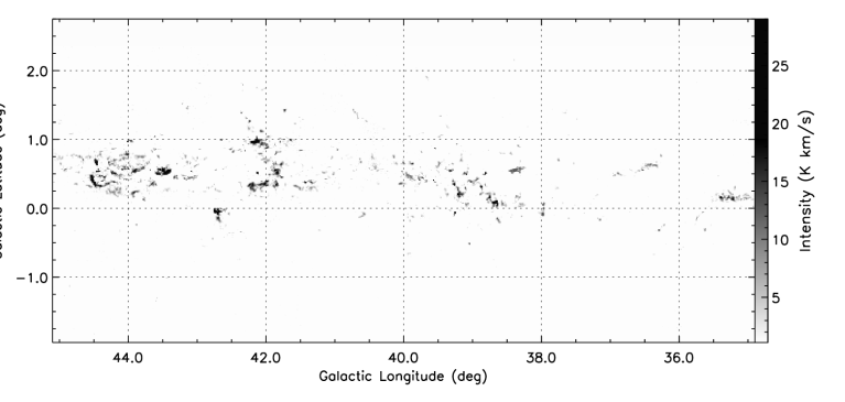
Figure 1.— ¹²CO ($J$=1–0) integrated intensity map of the MCs on the interval of $-1.6\times l$+$13.2\,{\rm km}\,{\rm s}^{-1}$ to $-10\,{\rm km}\,{\rm s}^{-1}$. Only $>3\times$rms points are accounted for.

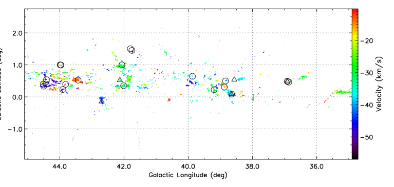
Figure 2.— Intensity-weighted mean velocity (first moment) map of the MCs from ¹²CO ($J$=1–0) emission on the interval of $-1.6\times l$+$13.2\,{\rm km}\,{\rm s}^{-1}$ to $-10\,{\rm km}\,{\rm s}^{-1}$. Only $>5\times$rms points are accounted for. The black circles and triangles are the positions of the 21 H ii regions and five 6.7 GHz masers from Table 3. The blue stripes at $l=$41$\fdg$5 and $b=-$1$\fdg$5 are from bad channels at $-41.59\,{\rm km}\,{\rm s}^{-1}$ (see the text).

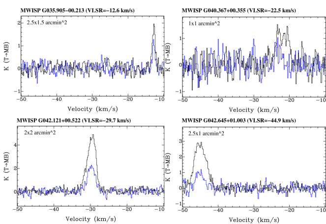
Figure 3.— Typical ¹²CO ($J$=1–0; black) and ¹³CO ($J$=1–0; blue, multiplied by a factor of two) spectra of the distant MCs. The extraction area of the spectra is shown in the top-left corner of each panel. The $Y$ axis is the main beam temperature of the MCs.

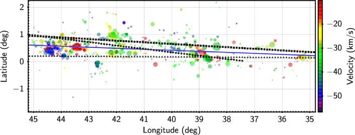
Figure 4.— Distribution of the 575 MCs in the Galactic coordinate system. The filled color circles are 575 MCs in Table 1 and are weighted with the scale of $L_{\rm CO}^{0.5}$. The thick blue line (weighted with the luminosity of the MC, $b$=0$\fdg$0377$\times l-$1$\fdg$0893) shows the best fit by a linear function. Circle-dotted line: warp model from Hi data ($m=1$ mode, refer to Levine et al., 2006); Box-dotted line: warp model from 2MASS star counts (Reylé et al., 2009); Triangle-dotted line: tilted-plane model from Hammersley et al. (1995).

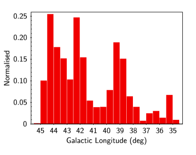
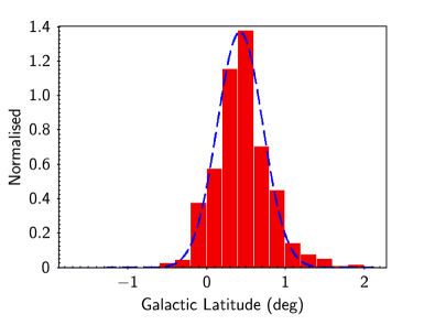
Figure 5.— Histograms of the 575 MCs with the Galactic longitude (the left panel) and latitude (the right panel). The dashed blue line in the right panel shows the best fit by a Gaussian function with the FWHM of $\sim$0$\fdg$7. The y axis is the fraction of the MCs weighted with their integrated intensity.

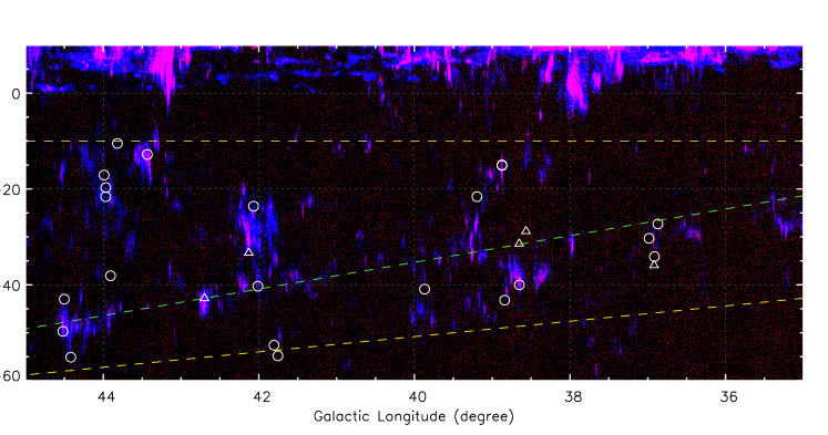
Figure 6.— PV diagram of the distant MCs with the Galactic longitude in the Galactic latitude range of $-$0$\fdg$5 to 1$\fdg$5. The blue and red emission is from the ¹²CO ($J$=1–0) and ¹³CO ($J$=1–0), respectively. The white circles and triangles are the same as those in Figure 2. The yellow dashed lines present the LSR velocity range of the Outer Arm: $V_{\rm LSR}=-1.6\times l+13.2\,{\rm km}\,{\rm s}^{-1}$ to $-10\,{\rm km}\,{\rm s}^{-1}$. The green dashed line indicates the longitude$-$velocity relation from the best fit of the ¹³CO ($J$=1–0) emission (excluding MCs near $l\sim 44^{\circ}$ and $V_{\rm LSR}\sim-20\,{\rm km}\,{\rm s}^{-1}$): $V_{\rm LSR}=-2.78\times l+75.9\,{\rm km}\,{\rm s}^{-1}$.

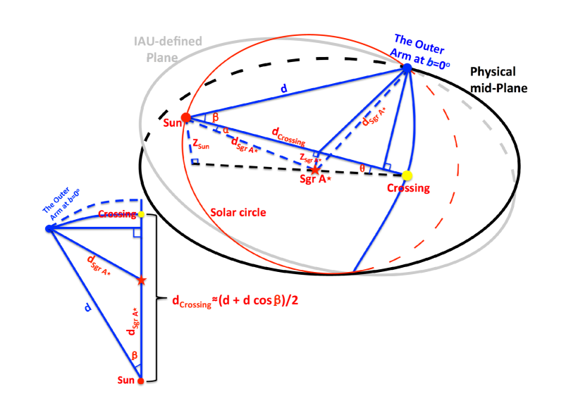
Figure 7.— Schematic diagram of the physical mid-plane of the Galaxy with respect to the IAU-defined plane of $b=0^{\circ}$. Note that the lines and the angles in the map are not to scale. All solid blue lines are in the IAU-defined plane $b=0^{\circ}$. The red ellipse indicates the solar circle. The Outer Arm, which traces the physical mid-plane in the first Galactic quadrant, passes through the IAU-defined plane at the direction of $l=\beta$ and $b=0^{\circ}$. $Z_{\rm Sun}$ and $Z_{\rm SgrA^{\star}}$ represent the height of the Sun above the physical mid-plane and the offset of the Galactic center (Sgr A^⋆) below the IAU-defined plane, respectively. The schematic face-on view of the geometrical relation, which is the projection onto the IAU-defined plane, is also shown in the lower left corner. Thus the value of $d_{\rm Crossing}$ is about 13.69 kpc. The $\alpha$, $\beta$, and the tilted angle $\theta$ are $-$0$\fdg$046, 28$\fdg$9, and 0$\fdg$072 (see the text), respectively. The derived $Z_{\rm Sun}$ is about 17.1 pc. In the calculation, the distance from the Sun to the Galactic center is $d_{\rm SgrA^{\star}}=$ 8.34 kpc.

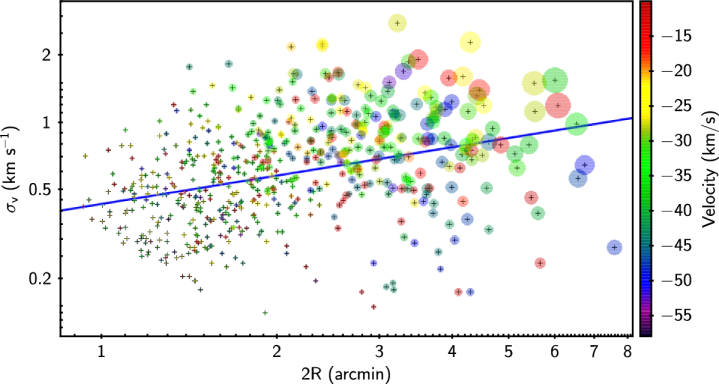
Figure 8.— MC velocity dispersion ($\sigma_{v}$=$\Delta V_{\rm FWHM}$/2.355) as a function of size ($2R$=2(Area/3.14)^1/2) for the 575 clouds in Table 1. The black crosses and the filled circles are for the fitted position and the scaled size of the MCs, respectively. The thick blue line ($\sigma_{v}\sim\rm{size}^{0.42}$, correlation coefficient (c.c.)=0.34) indicates the best fit by a power-law correlation.

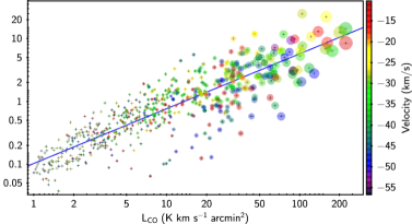
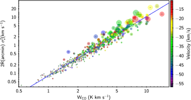
Figure 9.— Left: the CO luminosity ($L_{\rm CO}$)–virial mass ($M_{\rm virial}\sim 2R\times\sigma_{v}^{2}$) relation for the 575 MCs. The black crosses and the filled circles are the same as those in Figure 8. The thick blue line ($M_{\rm virial}\sim L_{\rm CO}^{0.87}$, c.c.=0.87) indicates the best fit by a power-law correlation. Right: the CO intensity ($W_{\rm CO}$)–virial mass ($M_{\rm virial}$) relation. The thick blue line ($M_{\rm virial}\sim W_{\rm CO}^{2.11}$, c.c.=0.98) indicates the best fit by a power-law correlation.

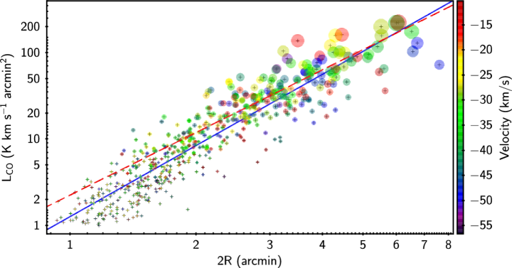
Figure 10.— Correlation between the size ($2R$) and the CO luminosity ($L_{\rm CO}$) of the 575 MCs. The black crosses and the filled circles are the same as those in Figure 8. The thick blue ($L_{\rm CO}\sim\rm{size}^{2.74}$, c.c.=0.92) and dashed red (weighted with the luminosity of the MC, $L_{\rm CO}\sim\rm{size}^{2.41}$, c.c.=0.90) lines indicate the best fit by a power-law correlation.

Table 1Parameters of 575 Molecular Clouds Identified from ¹²CO($J$=1–0) Emission

ID (1)	$l$ (∘) (2)	$b$ (∘) (3)	$V_{\rm LSR}$ ($\,{\rm km}\,{\rm s}^{-1}$) (4)	$\Delta V_{\rm FWHM}$ ($\,{\rm km}\,{\rm s}^{-1}$) (5)	$T_{\rm peak}$ (K) (6)	Area (arcmin2) (7)	$W_{\rm{}^{12}CO}$ (K $\,{\rm km}\,{\rm s}^{-1}$) (8)	$L_{\rm{}^{12}CO}$ (K $\,{\rm km}\,{\rm s}^{-1}$ arcmin2) (9)
001	34.913	0.025	-23.61	2.22	2.81	1.75	3.92	6.88
002	34.988	0.191	-24.71	1.08	2.68	1.47	1.86	2.73
003	34.991	0.147	-27.85	1.50	5.66	12.23	3.24	39.60
004	35.043	0.197	-12.39	0.80	2.60	2.33	1.38	3.23
005	35.082	0.137	-26.66	1.30	2.23	1.07	2.12	2.27
006	35.086	0.041	-18.33	0.85	2.28	1.86	1.45	2.70
007	35.136	0.164	-26.70	2.42	3.28	4.08	4.45	18.17
008	35.181	0.303	-38.35	2.51	2.73	2.74	4.29	11.75
009	35.248	0.152	-28.02	2.64	5.59	24.06	6.51	156.68
010	35.252	0.232	-22.39	2.00	4.36	8.33	4.44	36.93
011	35.287	0.090	-25.66	0.65	2.28	1.64	1.14	1.87
012	35.374	0.186	-14.85	2.64	4.53	5.44	5.87	31.94
013	35.375	0.149	-22.65	3.19	5.71	10.12	7.08	71.68
014	35.377	0.167	-27.45	0.65	2.41	1.58	1.14	1.81
015	35.421	0.472	-22.28	1.41	2.39	1.18	2.51	2.96
016	35.440	0.138	-24.43	0.59	2.34	1.48	1.01	1.49
017	35.442	0.206	-23.16	2.38	3.08	1.82	4.45	8.09
018	35.448	0.121	-12.25	1.41	2.72	2.00	2.60	5.20
019	35.449	0.239	-24.61	0.76	2.25	1.15	1.33	1.53
020	35.456	0.016	-11.90	1.06	2.69	2.62	1.92	5.04
021	35.471	-0.517	-42.42	0.68	2.35	1.11	1.19	1.32
022	35.506	0.115	-11.03	1.00	3.28	5.14	2.03	10.44
023	35.546	0.006	-11.09	0.48	2.63	1.49	0.79	1.17
024	35.609	-0.326	-23.95	1.09	2.18	1.02	1.79	1.83
025	35.613	-0.309	-26.06	2.09	3.04	3.23	3.71	12.00
026	35.704	-0.115	-11.69	1.47	4.58	13.29	3.25	43.26
027	35.905	-0.213	-12.57	0.53	3.25	3.96	1.06	4.21
028	35.927	-0.561	-11.13	1.11	3.08	1.57	1.94	3.04
029	35.958	-0.597	-13.27	1.77	2.26	0.83	2.92	2.42
030	36.210	-0.242	-42.84	1.90	3.24	1.81	3.44	6.24
031	36.250	-0.267	-37.65	1.36	2.35	1.11	2.37	2.64
032	36.255	0.768	-16.07	2.01	6.57	4.86	5.14	24.97
033	36.281	-0.315	-38.17	2.72	2.91	2.32	4.88	11.29
034	36.333	0.680	-26.65	1.52	3.26	1.91	2.69	5.13
035	36.353	-0.680	-19.20	0.97	2.93	2.12	1.73	3.67
036	36.368	0.631	-29.17	3.11	4.57	15.22	6.88	104.72
037	36.430	0.169	-26.16	1.66	2.15	0.69	2.73	1.89
038	36.441	0.578	-29.43	0.65	3.12	1.78	1.20	2.14
039	36.534	0.562	-27.23	1.96	4.19	5.66	4.05	22.94
040	36.618	0.529	-28.10	1.85	2.40	0.92	3.06	2.82
041	36.639	0.464	-20.56	1.04	2.50	2.14	1.88	4.02
042	36.703	0.567	-29.76	1.19	2.62	2.92	2.09	6.10
043	36.716	-0.054	-44.60	1.16	2.61	0.93	2.09	1.94
044	36.774	0.467	-26.30	0.58	1.90	1.42	0.92	1.30
045	36.822	-0.259	-10.48	0.68	2.69	1.69	1.30	2.20
046	36.857	0.504	-30.51	3.90	4.88	4.61	8.78	40.46
047	36.917	0.484	-31.68	1.90	5.57	2.91	5.57	16.20
048	36.929	0.485	-28.19	3.90	7.38	3.58	9.94	35.62
049	37.003	0.483	-25.55	0.92	2.51	0.95	1.49	1.41
050	37.136	-0.165	-11.46	1.46	7.20	5.91	4.12	24.37
051	37.174	-0.150	-37.53	1.38	3.62	2.42	2.83	6.85
052	37.191	0.195	-33.29	2.52	2.65	1.71	4.26	7.30
053	37.274	0.067	-14.11	0.69	2.70	1.67	1.18	1.96
054	37.506	0.053	-31.60	0.97	2.29	1.72	1.64	2.82
055	37.510	-0.217	-35.93	0.83	2.51	1.58	1.40	2.22
056	37.519	0.661	-29.68	1.33	4.22	3.66	2.90	10.63
057	37.594	-0.147	-36.81	1.32	3.67	3.13	2.77	8.68
058	37.643	1.408	-46.60	0.61	2.92	2.03	1.21	2.45
059	37.656	1.391	-44.24	1.01	2.70	3.17	1.69	5.36
060	37.747	0.709	-17.34	2.31	4.61	5.85	5.40	31.62

Table 2Parameters of 131 Molecular Clouds Identified from ¹³CO($J$=1–0) Emission

ID (1)	$l$ (∘) (2)	$b$ (∘) (3)	$V_{\rm LSR}$ ($\,{\rm km}\,{\rm s}^{-1}$) (4)	$\Delta V_{\rm FWHM}$ ($\,{\rm km}\,{\rm s}^{-1}$) (5)	$T_{\rm peak}$ (K) (6)	Area (arcmin2) (7)	$W_{\rm{}^{13}CO}$ (K $\,{\rm km}\,{\rm s}^{-1}$) (8)	$L_{\rm{}^{13}CO}$ (K $\,{\rm km}\,{\rm s}^{-1}$ arcmin2) (9)
001	34.971	0.159	-27.50	0.72	1.20	1.45	0.58	0.84
002	35.009	0.145	-28.25	1.08	1.99	2.12	1.02	2.17
003	35.145	0.152	-27.60	1.13	1.13	1.14	0.93	1.06
004	35.245	0.152	-28.33	2.48	1.87	5.39	2.21	11.93
005	35.250	0.230	-22.10	0.70	1.53	1.89	0.65	1.23
006	35.359	0.212	-13.66	1.21	1.29	1.13	0.97	1.09
007	35.380	0.159	-22.85	3.11	1.65	2.16	2.81	6.09
008	35.641	-0.059	-12.59	0.76	1.20	1.04	0.59	0.61
009	35.737	-0.148	-11.39	1.13	1.46	2.39	1.00	2.39
010	36.254	0.763	-16.23	0.88	1.24	1.65	0.73	1.21
011	36.344	0.633	-29.70	1.18	1.80	4.98	1.07	5.34
012	36.516	0.564	-27.04	0.98	1.72	1.78	0.86	1.53
013	36.833	0.488	-28.48	0.92	1.45	1.95	0.81	1.57
014	36.879	0.518	-31.74	1.29	1.43	1.48	1.02	1.51
015	36.919	0.488	-30.59	2.87	1.54	1.49	2.53	3.76
016	37.745	0.704	-17.56	1.48	2.07	3.21	1.45	4.66
017	37.963	0.064	-32.10	1.47	2.08	2.80	1.58	4.44
018	37.970	-0.089	-31.74	2.25	1.90	2.28	2.13	4.86
019	38.314	0.167	-17.13	0.71	1.15	1.23	0.58	0.71
020	38.357	0.181	-18.14	0.83	1.16	1.76	0.63	1.11
021	38.360	0.559	-38.12	2.03	1.68	5.32	1.76	9.35
022	38.418	0.527	-40.39	1.46	1.81	2.25	1.31	2.96
023	38.441	0.811	-38.79	1.04	1.06	1.63	0.78	1.27
024	38.632	-0.150	-39.75	1.98	1.66	1.70	1.79	3.04
025	38.655	0.083	-38.84	2.42	2.22	6.58	2.30	15.13
026	38.753	0.169	-38.05	3.17	2.54	3.43	3.27	11.21
027	38.771	0.100	-34.12	0.85	1.26	1.27	0.67	0.86
028	38.809	0.520	-40.98	1.90	2.24	2.42	1.97	4.76
029	38.869	0.312	-15.86	3.51	2.83	4.70	4.01	18.84
030	38.879	0.210	-35.50	1.15	1.36	2.16	1.00	2.17
031	38.928	0.436	-19.53	0.97	1.15	2.22	0.76	1.69
032	38.953	0.404	-46.58	0.48	1.02	1.65	0.37	0.60
033	39.013	0.387	-16.76	1.20	2.16	6.49	1.24	8.06
034	39.058	0.077	-16.48	0.86	1.45	1.60	0.76	1.22
035	39.088	0.064	-33.58	0.83	1.17	1.64	0.65	1.07
036	39.094	0.293	-44.99	1.42	1.32	2.05	1.26	2.57
037	39.148	0.199	-15.98	0.89	1.57	1.64	0.75	1.24
038	39.159	0.212	-34.27	1.14	1.15	1.16	0.87	1.01
039	39.198	0.208	-27.45	2.07	1.53	4.76	1.79	8.51
040	39.216	0.304	-27.36	0.92	1.69	2.39	0.80	1.91
041	39.256	-0.068	-33.50	1.60	2.77	6.32	1.96	12.35
042	39.265	0.352	-30.35	1.74	2.38	3.77	1.76	6.61
043	39.298	0.554	-43.40	1.34	1.15	1.58	1.04	1.65
044	39.318	-0.031	-32.41	0.70	1.12	1.12	0.54	0.61
045	39.323	0.552	-26.92	1.63	1.89	2.01	1.50	3.02
046	39.472	0.662	-32.52	1.22	1.09	1.19	0.92	1.10
047	39.508	0.611	-33.80	0.58	1.19	1.21	0.46	0.56
048	39.537	0.878	-38.26	0.84	1.42	1.39	0.72	0.99
049	39.661	1.910	-28.94	0.92	1.13	2.12	0.71	1.49
050	39.669	0.397	-34.82	1.00	1.70	3.40	0.91	3.11
051	39.727	0.511	-33.34	0.56	1.21	1.84	0.48	0.88
052	39.753	0.437	-47.74	1.41	1.68	2.18	1.16	2.52
053	39.860	-0.118	-32.89	0.96	1.27	1.00	0.79	0.79
054	39.870	0.658	-37.95	1.89	1.52	1.54	1.65	2.55
055	39.901	-0.175	-32.61	0.94	1.50	1.24	0.83	1.02
056	39.972	0.658	-35.32	0.77	0.87	0.86	0.56	0.48
057	40.017	0.540	-47.02	1.05	1.15	1.11	0.83	0.92
058	40.044	0.357	-44.52	0.55	1.12	1.51	0.46	0.70
059	40.135	0.753	-30.55	1.16	1.19	1.28	0.92	1.18
060	40.586	-0.093	-11.36	1.58	2.14	3.72	1.51	5.61

Table 3Molecular Clouds Associated with Massive Star Formation Regions

Name a	$l$ (∘)	$b$ (∘)	$V_{\rm MC}$ ($\,{\rm km}\,{\rm s}^{-1}$)	Tracers b,c	$l$ (∘)	$b$ (∘)	$V_{\rm LSR}$ ($\,{\rm km}\,{\rm s}^{-1}$)	References d
MWISP G036.833$+$00.488	36.833	0.488	-28.48	H ii G036.870$+$00.462	36.870	0.462	-27.3	(4)
MWISP G036.879$+$00.518	36.879	0.518	-31.74
MWISP G036.919$+$00.488	36.919	0.488	-30.59	H ii G036.914$+$00.489	36.984	0.489	-30.3	(1)
				H ii G036.914$+$00.485	36.914	0.485	-34.1	(4)
				Maser G36.918$+$0.483	36.918	0.483	-35.9	(6),(9)
MWISP G038.655$+$00.083	38.655	0.083	-38.84	H ii G038.651$+$00.087	38.651	0.087	-40.0	(4)
				Maser G38.653$+$0.088	38.653	0.088	-31.4	(6),(9)
MWISP G038.809$+$00.520	38.809	0.520	-40.98	H ii G038.840$+$00.497	38.840	0.497	-43.2	(4)
MWISP G038.869$+$00.312	38.869	0.312	-15.86	H ii G038.875$+$00.308	38.875	0.308	-15.1	(4)
				H ii G038.875$+$00.308	38.875	0.308	-14.98	(5)
MWISP G039.198$+$00.208	39.198	0.208	-27.45	H ii G039.195$+$00.226	39.195	0.226	-21.6	(7)
MWISP G039.870$+$00.658	39.870	0.658	-37.95	H ii G039.869$+$00.645	39.869	0.645	-40.9	(4)
MWISP G041.727$+$01.433	41.727	1.433	-50.88	H ii G041.755$+$01.451	41.755	1.451	-54.8	(8)
				H ii G041.804$+$01.503	41.804	1.503	-52.6	(8)
MWISP G041.982$+$00.342	41.982	0.342	-39.95	H ii G042.012$+$00.349	42.012	0.349	-40.3	(4)
MWISP G042.120$+$00.521	42.120	0.521	-29.76	Maser G42.13$+$0.52	42.13	0.52	-33.3	(9)
MWISP G042.150$+$00.982	42.150	0.982	-29.16	H ii G042.068$+$00.999	42.068	0.999	-23.6	(8)
MWISP G042.696$-$00.150	42.696	-0.150	-44.32	Maser G42.698$-$0.147	42.698	-0.147	-42.8	(6),(9)
MWISP G043.436$+$00.551	43.436	0.551	-14.06	H ii G043.432$+$00.521	43.432	0.521	-12.8	(4)
MWISP G043.909$+$00.239	43.909	0.239	-45.74	H ii G043.906$+$00.230	43.906	0.230	-38.1	(4)
MWISP G043.950$+$00.983	43.950	0.983	-29.68	H ii G043.968$+$00.993	43.968	0.993	-21.6	(4)
				H ii G043.989$+$01.000	43.989	1.000	-17.1	(8)
MWISP G044.415$+$00.465	44.415	0.465	-49.84	H ii G044.417$+$00.536	44.417	0.536	-55.1	(4)
MWISP G044.480$+$00.343	44.480	0.343	-48.99	H ii G044.501$+$00.335	44.501	0.335	-43.0	(4)
MWISP G044.559$+$00.326	44.559	0.326	-46.41
MWISP G044.518$+$00.396	44.518	0.396	-48.15	H ii G044.518$+$00.397	44.518	0.397	-49.7	(4)
MWISP G043.827$+$00.393 e	43.827	0.393	-12.17	H ii G043.818$+$00.393	43.818	0.393	-10.5	(4)
MWISP G043.957$+$00.998 e	43.957	0.998	-20.03	H ii G043.967$+$00.995	43.967	0.995	-19.7 f	(2),(3)

Note. — ^a Named from Galactic coordinates of the MCs from ¹³CO ($J$=1–0) emission (Table 2). The last two MCs in the table are from ¹²CO ($J$=1–0) emission (Table 1). ^b We use H ii regions and 6.7 GHz methanol masers to trace massive star formation regions. The position and the velocity of the H ii region is from the radio continuum emission and the radio recombination line, respectively. The position and the velocity of the 6.7 GHz maser is from the observations of the maser survey (Green & McClure-Griffiths, 2011; Breen et al., 2015). ^c Based on Tables 1 and 2, we do not find the CO counterpart of the 6.7 GHZ maser G38.565$+$0.538 with the LSR velocity of $-$28.8 $\,{\rm km}\,{\rm s}^{-1}$ (Table 1 in Breen et al., 2015). However, a point-like MC with a temperature of $\sim$1.5 K and the LSR velocity of $-$35.40 $\,{\rm km}\,{\rm s}^{-1}$ is detected from the ¹²CO ($J$=1–0) data at the maser’s position. ^d (1) Lockman, 1989; (2) Bronfman et al., 1996; (3) Gregory et al., 1996; (4) Anderson et al., 2011; (5) Balser et al., 2011; (6) Green & McClure-Griffiths, 2011; (7) Bania et al., 2012; (8) Anderson et al., 2015; (9) Breen et al., 2015. ^e The parameters of the MCs are from ¹²CO ($J$=1–0) emission (Table 1). ^f The velocity of the H ii region is from the CS ($J$=2–1) observation.

References

- Anderson et al. (2015) Anderson, L. D., Armentrout, W. P., Johnstone, B. M., et al. 2015, ApJS, 221, 26
- Anderson et al. (2011) Anderson, L. D., Bania, T. M., Balser, D. S., & Rood, R. T. 2011, ApJS, 194, 32
- Balser et al. (2011) Balser, D. S., Rood, R. T., Bania, T. M., & Anderson, L. D. 2011, ApJ, 738, 27
- Bania et al. (2012) Bania, T. M., Anderson, L. D., & Balser, D. S. 2012, ApJ, 759, 96
- Binney & Merrifield (1998) Binney, J., & Merrifield, M. 1998, Galactic Astronomy (Princeton, NJ: Princeton Univ. Press)
- Bobylev & Bajkova (2016) Bobylev, V. V., & Bajkova, A. T. 2016, Astronomy Letters, 42, 1
- Bolatto et al. (2013) Bolatto, A. D., Wolfire, M., & Leroy, A. K. 2013, ARA&A, 51, 207
- Bottema (1996) Bottema, R. 1996, A&A, 306, 345
- Brand & Blitz (1993) Brand, J., & Blitz, L. 1993, A&A, 275, 67
- Breen et al. (2015) Breen, S. L., Fuller, G. A., Caswell, J. L., et al. 2015, MNRAS, 450, 4109
- Bronfman et al. (1996) Bronfman, L., Nyman, L.-A., & May, J. 1996, A&AS, 115, 81
- Burke (1957) Burke, B. F. 1957, AJ, 62, 90
- Burton et al. (2013) Burton, M. G., Braiding, C., Glueck, C., et al. 2013, PASA, 30, 44
- Burton (1988) Burton, W. B. 1988, Galactic and Extragalactic Radio Astronomy (Berlin and New York, Springer-Verlag), ed. K. I. Kellermann & G. L. Verschuur, 295–358
- Chen et al. (2001) Chen, B., Stoughton, C., Smith, J. A., et al. 2001, ApJ, 553, 184
- Clemens (1985) Clemens, D. P. 1985, ApJ, 295, 422
- Clemens et al. (1988) Clemens, D. P., Sanders, D. B., & Scoville, N. Z. 1988, ApJ, 327, 139
- Clemens et al. (1986) Clemens, D. P., Sanders, D. B., Scoville, N. Z., & Solomon, P. M. 1986, ApJS, 60, 297
- Dame et al. (1986) Dame, T. M., Elmegreen, B. G., Cohen, R. S., & Thaddeus, P. 1986, ApJ, 305, 892
- Dame et al. (2001) Dame, T. M., Hartmann, D., & Thaddeus, P. 2001, ApJ, 547, 792
- Dame & Thaddeus (1985) Dame, T. M., & Thaddeus, P. 1985, ApJ, 297, 751
- Dame & Thaddeus (2011) —. 2011, ApJ, 734, L24
- Dame et al. (1987) Dame, T. M., Ungerechts, H., Cohen, R. S., et al. 1987, ApJ, 322, 706
- Dempsey et al. (2013) Dempsey, J. T., Thomas, H. S., & Currie, M. J. 2013, ApJS, 209, 8
- Digel et al. (1990) Digel, S., Thaddeus, P., & Bally, J. 1990, ApJ, 357, L29
- Drimmel & Spergel (2001) Drimmel, R., & Spergel, D. N. 2001, ApJ, 556, 181
- Du et al. (2016) Du, X., Xu, Y., Yang, J., et al. 2016, ApJS, 224, 7
- Elmegreen & Falgarone (1996) Elmegreen, B. G., & Falgarone, E. 1996, ApJ, 471, 816
- Foster & Cooper (2010) Foster, T., & Cooper, B. 2010, in Astronomical Society of the Pacific Conference Series, Vol. 438, The Dynamic Interstellar Medium: A Celebration of the Canadian Galactic Plane Survey, ed. R. Kothes, T. L. Landecker, & A. G. Willis, 16
- Freudenreich (1998) Freudenreich, H. T. 1998, ApJ, 492, 495
- Freudenreich et al. (1994) Freudenreich, H. T., Berriman, G. B., Dwek, E., et al. 1994, ApJ, 429, L69
- Goodman et al. (2014) Goodman, A. A., Alves, J., Beaumont, C. N., et al. 2014, ApJ, 797, 53
- Green & McClure-Griffiths (2011) Green, J. A., & McClure-Griffiths, N. M. 2011, MNRAS, 417, 2500
- Gregory et al. (1996) Gregory, P. C., Scott, W. K., Douglas, K., & Condon, J. J. 1996, ApJS, 103, 427
- Hammersley et al. (1995) Hammersley, P. L., Garzon, F., Mahoney, T., & Calbet, X. 1995, MNRAS, 273, 206
- Henderson et al. (1982) Henderson, A. P., Jackson, P. D., & Kerr, F. J. 1982, ApJ, 263, 116
- Heyer & Dame (2015) Heyer, M., & Dame, T. M. 2015, ARA&A, 53, 583
- Heyer et al. (2009) Heyer, M., Krawczyk, C., Duval, J., & Jackson, J. M. 2009, ApJ, 699, 1092
- Heyer et al. (2001) Heyer, M. H., Carpenter, J. M., & Snell, R. L. 2001, ApJ, 551, 852
- Heyer & Terebey (1998) Heyer, M. H., & Terebey, S. 1998, ApJ, 502, 265
- Humphreys & Larsen (1995) Humphreys, R. M., & Larsen, J. A. 1995, AJ, 110, 2183
- Jackson et al. (2006) Jackson, J. M., Rathborne, J. M., Shah, R. Y., et al. 2006, ApJS, 163, 145
- Jacq et al. (1988) Jacq, T., Despois, D., & Baudry, A. 1988, A&A, 195, 93
- Joshi (2007) Joshi, Y. C. 2007, MNRAS, 378, 768
- Kutner & Mead (1981) Kutner, M. L., & Mead, K. N. 1981, ApJ, 249, L15
- Larson (1981) Larson, R. B. 1981, MNRAS, 194, 809
- Levine et al. (2006) Levine, E. S., Blitz, L., & Heiles, C. 2006, ApJ, 643, 881
- Lockman (1989) Lockman, F. J. 1989, ApJS, 71, 469
- López-Corredoira et al. (2002) López-Corredoira, M., Cabrera-Lavers, A., Garzón, F., & Hammersley, P. L. 2002, A&A, 394, 883
- Maíz-Apellániz (2001) Maíz-Apellániz, J. 2001, AJ, 121, 2737
- Majaess et al. (2009) Majaess, D. J., Turner, D. G., & Lane, D. J. 2009, MNRAS, 398, 263
- McClure-Griffiths & Dickey (2007) McClure-Griffiths, N. M., & Dickey, J. M. 2007, ApJ, 671, 427
- Mead & Kutner (1988) Mead, K. N., & Kutner, M. L. 1988, ApJ, 330, 399
- Nakanishi & Sofue (2003) Nakanishi, H., & Sofue, Y. 2003, PASJ, 55, 191
- Nakanishi & Sofue (2006) —. 2006, PASJ, 58, 847
- Oort et al. (1958) Oort, J. H., Kerr, F. J., & Westerhout, G. 1958, MNRAS, 118, 379
- Reed (2006) Reed, B. C. 2006, JRASC, 100, 146
- Reid & Brunthaler (2004) Reid, M. J., & Brunthaler, A. 2004, ApJ, 616, 872
- Reid et al. (2016) Reid, M. J., Dame, T. M., Menten, K. M., & Brunthaler, A. 2016, ApJ, 823, 77
- Reid et al. (2014) Reid, M. J., Menten, K. M., Brunthaler, A., et al. 2014, ApJ, 783, 130
- Reshetnikov et al. (2002) Reshetnikov, V., Battaner, E., Combes, F., & Jiménez-Vicente, J. 2002, A&A, 382, 513
- Reshetnikov & Combes (1998) Reshetnikov, V., & Combes, F. 1998, A&A, 337, 9
- Reylé et al. (2009) Reylé, C., Marshall, D. J., Robin, A. C., & Schultheis, M. 2009, A&A, 495, 819
- Roman-Duval et al. (2010) Roman-Duval, J., Jackson, J. M., Heyer, M., Rathborne, J., & Simon, R. 2010, ApJ, 723, 492
- Schwarzkopf & Dettmar (2001) Schwarzkopf, U., & Dettmar, R.-J. 2001, A&A, 373, 402
- Scoville et al. (1987) Scoville, N. Z., Yun, M. S., Sanders, D. B., Clemens, D. P., & Waller, W. H. 1987, ApJS, 63, 821
- Shan et al. (2012) Shan, W. L., Yang, J., Shi, S. C., et al. 2012, IEEE Transactions on Terahertz Science and Technology, 2, 593
- Solomon & Rivolo (1989) Solomon, P. M., & Rivolo, A. R. 1989, ApJ, 339, 919
- Solomon et al. (1987) Solomon, P. M., Rivolo, A. R., Barrett, J., & Yahil, A. 1987, ApJ, 319, 730
- Stil et al. (2006) Stil, J. M., Taylor, A. R., Dickey, J. M., et al. 2006, AJ, 132, 1158
- Sun et al. (2015) Sun, Y., Xu, Y., Yang, J., et al. 2015, ApJ, 798, L27
- Taylor (2005) Taylor, M. B. 2005, in Astronomical Society of the Pacific Conference Series, Vol. 347, Astronomical Data Analysis Software and Systems XIV, ed. P. Shopbell, M. Britton, & R. Ebert, 29
- Vallée (2014) Vallée, J. P. 2014, ApJS, 215, 1
- Williams et al. (1994) Williams, J. P., de Geus, E. J., & Blitz, L. 1994, ApJ, 428, 693
- Xu et al. (2013) Xu, Y., Li, J. J., Reid, M. J., et al. 2013, ApJ, 769, 15
- Zhang et al. (2014) Zhang, S., Xu, Y., & Yang, J. 2014, AJ, 147, 46