Associative memory by collective regulation of non-coding RNA

Abstract

The majority of mammalian genomic transcripts do not directly code for proteins and it is currently believed that most of these are not under evolutionary constraint. However given the abundance non-coding RNA (ncRNA) and its strong affinity for inter-RNA binding, these molecules have the potential to regulate proteins in a highly distributed way, similar to artificial neural networks. We explore this analogy by devising a simple architecture for a biochemical network that can function as an associative memory. We show that the steady state solution for this chemical network has the same structure as an associative memory neural network model. By allowing the choice of equilibrium constants between different ncRNA species, the concentration of unbound ncRNA can be made to follow any pattern and many patterns can be stored simultaneously. The model is studied numerically and within certain parameter regimes it functions as predicted. Even if the starting concentration pattern is quite different, it is shown to converge to the original pattern most of the time. The network is also robust to mutations in equilibrium constants. This calls into question the criteria for deciding if a sequence is under evolutionary constraint.

I Introduction

Non-coding RNA (ncRNA) has emerged in recent years as a major player in the molecular biology of the cell. The vast majority of transcripts in the cell produce long (greater than 200 nucleotides) non-coding RNA, and many of their functions have been studied ENCODEpilot ; Kapranov2007 ; MercerDingerMattick ; ENCODE . A recent paper Deutsch14 proposed that a function of much of the non-coding RNA thought not to be under evolutionary constraint, was to act collectively to regulate protein transcription. Instead of individual genes being controlled by a few regulatory elements, ncRNA acts collectively to control transcription. If we assume weak binding of many species of ncRNA to each other, the amount of unbound ncRNA depends on all of the other species collectively. This free ncRNA can then act to regulate mRNA in a variety of possible ways. The important distinction between this behavior and other regulatory mechanisms, such as cis-regulation, is the collective nature of regulation.

In computer science, it has been known for many decades, that it is possible to make intelligent computational decisions using distributed networks, and these form the bulk of models for artificial and real neural network HertzKroghPalmer . This differs from most digital circuitry in that the output is computed using network elements that interact with many others in a robust way. This means that even if connection strengths are varied or even eliminated entirely, the network will still keep much of its original function. This is an advantage over traditional computer circuitry which has a much sparser connectivity. Furthermore this architecture is well suited to learning new tasks.

In this paper, we devise a ncRNA system that will behave as an associative memory. The model behaves in a similar manner to associative memory neural networks LittleShaw ; Hopfield ; AmitGutFreundSompolinsky . There are two ingredients to this system: (i) A regulated mechanism to produce many species of ncRNA molecules, that will degrade at some rate over time, (ii) The ncRNA molecules bind and unbind with equilibrium constants that can be varied by changing the sequence of them. We assume that the regulation will depend on the total concentration of ncRNA, and the amount of unbound ncRNA. We find a specific functional form for the regulation of ncRNA that leads to nonlinear self-consistent equations for unbound ncRNA concentrations. These equations are essentially the same as what is used in associative memory models.

There are three caveats to this scenario however. The first is that the relaxation time for the chemical equilibration of the ncRNA is much shorter than the time it takes to degrade ncRNA molecules. The second, is that we have given the mathematical form for the regulation of ncRNA that depends on different ncRNA concentrations, but we have not provided a physical or chemical model that can implement this precisely. Similar regulation takes place but its precise form is still not understood well quantitatively. Finally, it requires that we have complete freedom to choose the equilibrium constants between different species.

As with many neural network and statistical mechanical models, the precise form of a model often does not matter HertzKroghPalmer , and we expect that a range of models will have similar behavior. This model does not imply that precisely this biochemical mechanism exists, but rather it shows the existence of mechanisms that are relatively simple, and can result in collective regulation of the genome in a manner quite unlike the ones that have already been discovered. This work makes such a paradigm more plausible.

II The model

Here we study how regulating the transcription of $N$ species of non-coding RNA (ncRNA), combined with the promiscuous binding of ncRNA species to each other, can lead to an associative memory. We denote the total concentration of of the $N$ species by $C_{1},C_{2},\dots,C_{N}$, and the unbound concentrations $\rho_{1},\rho_{2},\dots,\rho_{N}$.

II.1 Model Assumptions

II.1.1 Assumptions about binding

We assume that the standard form for chemical reactions between different species, $i$, and $j$

$$i+j\rightleftharpoons ij$$ (1)

We are assuming here that these are the only kinds of reaction present. There are no higher order reactions involving three or more species.

We can define an equilibrium constant Reif $K_{i,j}=\rho_{ij}/\rho_{i}\rho_{j}$. Here $\rho_{ij}$ is the concentration of bound molecules $ij$. This leads to Deutsch14

$$\rho_{i}=\frac{C_{i}}{1+\sum_{j}\rho_{j}K_{i,j}}$$ (2)

for $i=1,\dots,N$.

We further assume that we have complete freedom to choose the equilibrium constants. That is, there is enough choice in the sequences and binding positions of the RNA molecules that the equilibrium constant of one pair does not influence another one.

II.1.2 Assumptions about molecular regulation

The concentration of an individual species of ncRNA needs to be regulated for the mechanism described here to work. Regulation is expected for biochemical processes, however we require more specifically that the regulation should depend on the current total concentration $C$, as well as the concentration of unbound ncRNA $\rho$. $\rho$ can be measured with the assumption that only the unbound molecules will be able to bind to a particular RNA binding biomolecule (such as a protein) involved in the regulation of this kind of ncRNA. The total concentration $C$, can be measured with the assumption that there is another biomolecule that binds to a different portion on the ncRNA which is normally not associated with another RNA molecule, for example because it is in a stem loop. An example of such a protein is a stem-loop binding protein (SLBP).

If both unbound and bound ncRNA concentrations are directly related to the concentrations of certain proteins that bind to them as suggested above, it would appear feasible that a complex of such proteins could evolve to produce transcription machinery that allows regulation in the way we hypothesize below. This seems reasonable because well known genetic regulatory mechanisms are well tuned to both enhance and suppress transcription. We are only requiring that individual components enhancing and suppressing transcription can be combined to mimic the smooth dependence on $\rho$ and $C$ that is used here.

II.2 Dynamics of concentration and transcription rates

Eq. 2 relates the unbound concentration of one species to its total concentration, and the unbound concentration of all the other species. The system will start off out of equilibrium and we assume that it approaches it with a simplified first order kinetic equation

$$\tau_{\rho}\frac{d\rho_{i}}{dt}=-\rho_{i}+\frac{C_{i}}{1+\sum_{j}\rho_{j}K_{i,j}}$$ (3)

for $i=1,\dots,N$, where $\tau_{\rho}$ is a relaxation time, giving the time scale for the relaxation of the $\rho_{i}$’s to equilibrium.

As discussed above, the concentrations $C_{i}$ are regulated. We assume that individual molecules degrade over a timescale $\tau_{C}$, but are also being transcribed, leading to a non-zero steady state concentration. We assume that the degradation is a first order process, and the transcription of new ncRNA molecules is a function that depends on $C_{i}$ and all of the $\rho$’s.

$$\tau_{C}\frac{dC_{i}}{dt}=-C_{i}+f(C_{i},\{\rho_{k}\})$$ (4)

Physically we expect that $\tau_{C}\gg\tau_{\rho}$, that is, the degradation of the RNA happens at a much slower rate than equilibration of the binding and unbinding of RNA. $f$ represents the rate at which new transcripts are being produced. This could be accomplished by regulating the transcription through a variety of means, such as repressors or coactivators that can sense unbound and bound concentrations as discussed above.

We now choose a specific form of the function $f$ that will lead to an associative biochemical memory.

$$f(C_{i},\{\rho_{k}\})=\frac{C_{i}}{\rho_{i}}S(4\frac{C_{i}}{\rho_{i}}-2\sum_{j}(K_{i,j}+\rho_{j})-3N)$$ (5)

for $i=1,\dots,N$. The function $S(x)$ is a sigmoid function that could take a variety of forms, such as a logit function

$$S(x)=\frac{1}{2}[1+\tanh(\beta x/N)]$$ (6)

where $\beta$ is a constant, that in analogy to spin systems, represents an inverse temperature. We shall discuss its value below when we discuss the numerical implementation of this model.

Eqs. 3, 4, 5, and 6 define the dynamics of the $2N$ concentrations given a set of equilibrium constants $K_{i,j}$, and the initial conditions.

III Analysis

In steady state, all time derivatives vanish, and Eqs 3 reduces to 2. It can be rearranged to yield:

$$\sum_{j}K_{i,j}\rho_{j}=\frac{C_{i}}{\rho_{i}}-1$$ (7)

Eq. 4 reduces to

$$C_{i}=f(C_{i},\{\rho_{k}\})$$ (8)

If we transform to symmetric variables $s_{i}$, $i=1,\dots,N$ so that $\rho_{i}=(1+s_{i})/2$. We will also choose symmetrized variables $J_{i,j}$ so that

$$K_{i,j}=\frac{1+J_{i,j}}{2}.$$ (9)

Substituting this into Eq. 5 and using Eq. 7 gives

$$C_{i}=f(C_{i},\{s_{k}\})=\frac{C_{i}}{1+s_{i}/2}S(\frac{1}{N}\sum_{j}J_{i,j}s_{j})$$ (10)

Canceling the $C_{i}$’s solving for $s_{i}$, and substituting Eq. 6 finally gives

$$s_{i}=\tanh(\frac{\beta}{N}\sum_{j}J_{i,j}s_{j})$$ (11)

Note that there is no guarantee that the dynamics of this system will lead to these steady state solutions as some of these may be unstable. But for the physically sensible requirement that we have imposed on the relaxation times, we will see below that these solutions are achieved.

This self consistent equation is used in analyzing neural network associative memories LittleShaw ; Hopfield ; AmitGutFreundSompolinsky and can have many solutions, depending on the choice of the $J$’s. We will now focus on the most common choice, that of Hebbian learning Hebb ; LittleShaw ; Hopfield .

III.1 Hebbian coupling

We can choose the $K$’s or equivalently the $J$’s in a manner that will allow the network to retrieve $M$ patterns. The retrieval works best when the patterns are uncorrelated. Let us denote the $\alpha$th pattern by $t_{i}^{\alpha}$, $\alpha=1,\dots,M$. We let each $t_{i}^{\alpha}=\pm 1$. Then

$$J_{i,j}=\frac{1}{M}\sum_{\alpha=1}^{M}t_{i}^{\alpha}t_{j}^{\alpha}$$ (12)

The number of patterns that can be reliably stored is proportional to $N$ AmitGutFreundSompolinsky but this will also depend on the correlations between the patterns.

In order for this choice to be physically meaningful, the $K$’s must all be positive. This is why we chose to relate the $K$’s to the $J$’s in the first place through Eq. 9. After choosing $M$ patterns and setting the $J$’s accordingly, they are shifted and scaled to produce positive $K$’s. $K\rightarrow K-min(K)$, and $K\rightarrow K/max(K)$. This produces equilibrium constants between zero and one.

III.2 Numerical results

The above model was implemented numerically. We chose $N=50$ ncRNA species, and analyze the retrieval $M=3$ separate patterns using the Hebbian rule of Eq. 12.

The ratio of the two timescales $\tau_{C}/\tau_{\rho}$ was found to be important in the convergence of this system. With $\tau_{C}/\tau_{\rho}=100$ the system always appeared to converge. However with $\tau_{C}/\tau_{\rho}=10$, it sometimes did not.

We tested out the basin of attraction of initial values of the $\rho_{i}$’s. We considered each pattern $t^{\alpha}$ and then randomly altered its sequence by varying amounts. For each ncRNA species, we chose a random number between zero and 1 flipped the value of the density $\rho_{i}\rightarrow 1-\rho_{i}$, if the random number was below some cutoff. We tried $5$ different mutations for each of the $M$ patterns, for a fixed cutoff. We generated $10$ separate examples of the $M$ patterns, and varied the cutoff. We plot the fraction of mistakes as a function of this cutoff in Fig 1. The three graphs represents three different values of $\beta$: $6$, $7$, and $8$. It is evident that for $\beta$ equals $6$, or $7$, some patterns are not stable, because even with a cutoff of zero leads in some cases to the system moving away to a different pattern. However, with $\beta=8$, all patterns were stable.

Next we tested out the effects of mutating the equilibrium constants $K_{i,j}$. We chose random $i$’s and $j^{\prime}s$ and mutated them by taking $K_{i,j}\rightarrow 1-K_{i,j}$, maintaining symmetry of the matrix. (Recall that $0<=K_{i,j}<=1$). We measured how close the final fixed point was to the original pattern, by measuring the Hamming distance between the two and dividing by $N$. We varied the number of $K$’s that were mutated. We ran this for the same number of times as above, and for the same values of $\beta$. The results are shown in Fig. 2. Even with $100$ mutations, most of a pattern is correctly recalled. This illustrates that this architecture is robust to mutations.

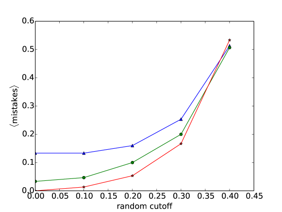
Figure 1: The number of mistakes made as a function of the distance away from a pattern. When the initial condition for the density is sufficiently different from the pattern, the system will move away from it towards a different to a different pattern. The red curve (stars) shows $\beta=8$, the green (circles), $\beta=7$, and the blue (triangles) $\beta=6$. The lines are a guide for the eye.

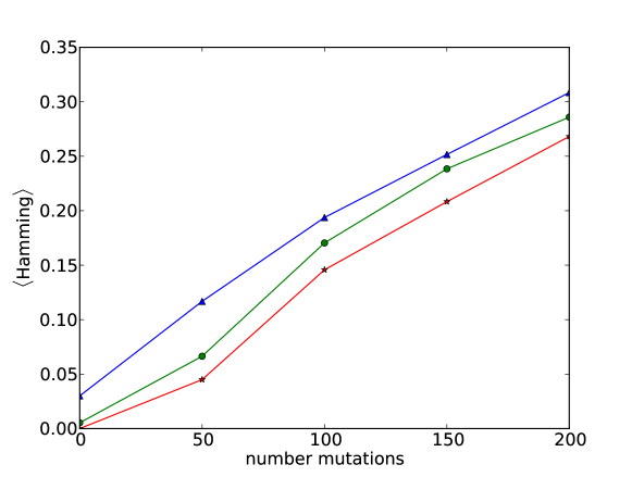
Figure 2: The effects of mutations to the equilibrium constants. The horizontal axis gives the number of mutations that were made. The vertical axis is the average fraction of errors, measured by the fractional Hamming distance of the desired pattern to the recalled pattern. This represents the fraction of incorrect concentration levels. The red curve (stars) shows $\beta=8$, the green (circles), $\beta=7$, and the blue (triangles) $\beta=6$. The lines are a guide for the eye.

.

IV Discussion

Here we have developed and analyzed a model for ncRNA that produces features of an associative memory which assumes promiscuous binding of many species to each other. We mapped the fixed points of this biochemical network onto a neural network model. However the stability of these points depends on two relaxation times, one for ncRNA equilibration, and the other characterizing the degradation time of ncRNA molecules. Furthermore the switching on of ncRNA transcription must be a sharp enough function of ncRNA concentrations, that is, have high enough $\beta$ (see Eq. 6), for the fixed points to be stable.

Although an associative memory has been considered here mainly as a gross simplification of a real genetic network, in order to elucidate, in detail, how genetic networks could make use of collective regulation, it is possible that this kind of behavior could be useful in an organism. In a neural network, if some fraction of a pattern is shown to an associative memory, the rest of it will be reproduced. Similarly for a genetic network, if some ncRNA species are presented to the network at given concentrations, the network will recognize this sub-“pattern”, and produce the additional pattern of ncRNA molecules at desired concentrations. Multiple patterns can be stored, meaning that the network can respond appropriately to different environmental conditions.

There are many advantages to distributed network computation and one would expect, as argued here, that these would carry over to networks used for genetic regulation. The robustness to mutation is one such feature. This means that mutations of ncRNA will have a much gentler effect than for sparse networks, but nevertheless could confer evolutionary advantages. This is important because much ncRNA is thought not to be under evolutionary constraint but in light of the above, this may be an incorrect conclusion. Much larger mutation rates for molecules utilizing collective regulation are expected even if they are involved in important regulatory functions. Therefore the mutation rate criteria for evolutionary pressure should be questioned to take this kind of collective mechanism.

The robustness of collective regulations to changes also means that it is difficult to come up with experimental means to find it, as each pairwise interactions between species are small and removal of individual interactions will not be easily noticed.

This model was not evolutionary, as this would make analysis intractable analytically. However it is straightforward to see how evolution would give rise to equilibrium constants that could store multiple patterns. Indeed, this is the similar to what is done with “Boltzmann machines” HertzKroghPalmer , where the network is trained with Monte Carlo on multiple patterns and eventually learns to respond to all of them correctly. The couplings will not end up being precisely those of Eq. 12, but they will achieve the same goal. Therefore we expect that an architecture such as described here, that evolves by mutating the $K_{i,j}$’s will produce similar behavior.

This work was supported by the Foundational Questions Institute <http://fqxi.org>.

References

- (1) The ENCODE Project Consortium, “Identification and analysis of functional elements in 1% of the human genome by the ENCODE pilot project”, Nature 447 799-816 (2007).
- (2) P. Kapranov, J Cheng, S. Dike, et al. “RNA maps reveal new RNA classes and a possible function for pervasive transcription”. Science 316 1484–8 (2007).
- (3) T. R. Mercer, M. E. Dinger and J. S. Mattick “Long non-coding RNAs: insights into functions” Nature Reviews Genetics 10, 155-159 (2009).
- (4) The ENCODE Project Consortium, “An integrated encyclopedia of DNA elements in the human genome” Nature 489 57-74 (2012).
- (5) J.M. Deutsch, “Collective regulations by non-coding RNA” arXiv:1409.1899 (2014).
- (6) J. Hertz, A. Krogh, and Palmer, R.G. “Introduction to the theory of neural computation.” Redwood City, CA: Addison-Wesley (1991).
- (7) W. A. Little, Math. Biosci. 19 101 (1974); W. A. Little and G. L. Shaw, Behav. Biol. 14115 (1975);Math. Biosci. 39 281 (1978).
- (8) J. J. Hopfield, Proc. Natl. Acad. Sci. USA 79, 2554-2558 (1982).
- (9) D.J Amit, H. Gutfreund and H. Sompolinksy, Phys. Rev. A, 32 1007-1018 (1985).
- (10) F. Reif “Fundamentals of statistical and thermal physics” McGraw-Hill (1965) Section 8.10.
- (11) D.O. Hebb, ”The Organization of Behavior.” New York: Wiley, (1949).