Solving the ⁵⁶Ni puzzle of magnetar-powered broad-lined type Ic supernovae

Abstract

Broad-lined type Ic supernovae (SNe Ic-BL) are of great importance because their association with long-duration gamma-ray bursts (LGRBs) holds the key to deciphering the central engine of LGRBs, which refrains from being unveiled despite decades of investigation. Among the two popularly hypothesized types of central engine, i.e., black holes and strongly magnetized neutron stars (magnetars), there is mounting evidence that the central engine of GRB-associated SNe (GRB-SNe) is rapidly rotating magnetars. Theoretical analysis also suggests that magnetars could be the central engine of SNe Ic-BL. What puzzled the researchers is the fact that light curve modeling indicates that as much as $0.2-0.5$ solar mass of ⁵⁶Ni was synthesized during the explosion of the SNe Ic-BL, which is unfortunately in direct conflict with current state-of-the-art understanding of magnetar-powered ⁵⁶Ni synthesis. Here we propose a dynamic model of magnetar-powered SNe to take into account the acceleration of the ejecta by the magnetar, as well as the thermalization of the injected energy. Assuming that the SN kinetic energy comes exclusively from the magnetar acceleration, we find that although a major fraction of the rotational energy of the magnetar is to accelerate the SNe ejecta, a tiny fraction of this energy deposited as thermal energy of the ejecta is enough to reduce the needed ⁵⁶Ni to 0.06 solar mass for both SNe 1997ef and 2007ru. We therefore suggest that magnetars could power SNe Ic-BL both in aspects of energetics and of ⁵⁶Ni synthesis.

1. Introduction

It is widely accepted that the death of massive stars should trigger core-collapse supernovae (CCSNe; Bethe, 1990; Janka, 2012) that can be classified as types IIP, IIL, IIn, IIb, Ib and Ic (Filippenko, 1997). In the last two decades, some SNe Ic having broader P-Cygni profiles and absorption troughs than normal SNe Ic were confirmed and nominated as “broad-lined SNe” (SNe Ic-BL; Woosley & Bloom, 2006).

Some SNe Ic-BL are associated with gamma-ray bursts (GRBs) or X-ray flashes (XRFs; Woosley & Bloom, 2006; Cano et al., 2016b). The association of LGRBs with SNe Ic-BL provides a unique channel to study the central engine of GRBs. Before the discovery of SNe Ic-BL, the majority of conventional SNe has a kinetic energy of $\sim 10^{51}\mathord{\thinspace\rm erg}$, which is generally attributed to neutrino energy deposition (Woosley et al., 2002; Janka, 2012). The huge amount of kinetic energy of SNe Ic-BL, $\sim 10^{52}\mathord{\thinspace\rm erg}$, poses an immediate challenge to this canonical SN picture.

One way to generate such a tremendous kinetic energy is to assume that the explosion remnant is a rapidly rotating magnetar (Wheeler et al., 2000; Thompson et al., 2004; Wang et al., 2016b), whose rotational energy is converted as the kinetic energy of SNe Ic-BL. Indeed, it is found that the kinetic energies of SNe Ic-BL associated with LGRBs are clustered at $10^{52}\mathord{\thinspace\rm erg}$ with an upper limit of $\sim 2\times 10^{52}\mathord{\thinspace\rm erg}$ (Mazzali et al., 2014), namely the maximum rotational energy of magnetars. This is a strong clue that GRB-SNe are powered by millisecond magnetars. In addition, the light curve of SN 2011kl associated with the ultra-long GRB 111209A suggests the existence of magnetar because ⁵⁶Ni is inadequate to reproduce the observational data (Greiner et al., 2015).

Light curve modeling of SNe Ic-BL indicates the synthesis of ⁵⁶Ni as massive as $M_{\mathrm{Ni}}=0.2-0.5M_{\odot}$, where $M_{\odot}$ is the solar mass. However, theoretical studies found that it is very difficult to synthesize $0.2M_{\odot}$ of ⁵⁶Ni by a millisecond magnetar with parameters given in the literature (Nishimura et al., 2015; Suwa & Tominaga, 2015). This conflict is a big concern to accept the hypothesis that SNe Ic-BL are powered by magnetars.

In arriving at the conclusion that SNe Ic-BL must have synthesized as massive as $0.2-0.5M_{\odot}$ of ⁵⁶Ni when modeling the SN light curves, one usually assumes that the SN thermal energy comes exclusively from the thermalization of the gamma-rays from the decay of ⁵⁶Ni and ⁵⁶Co. This assumption is correct if the thermalization of the (assumed) magnetar spin-down power can be neglected compared to the energy deposition from the decay of ⁵⁶Ni and ⁵⁶Co, as in the case of ordinary SNe Ic.

In the magnetar model for optical transients, it is well known that the contribution of magnetar to the SN thermal emission dominates over other (possible) energy sources in the case of superluminous SNe (SLSNe; Kasen & Bildsten, 2010; Woosley, 2010; Chatzopoulos et al., 2012, 2013; Inserra et al., 2013; Nicholl et al., 2014; Metzger et al., 2015; Wang et al., 2016c, 2015b; Dai et al., 2016; Kashiyama et al., 2016). Even for luminous SNe, whose luminosities lie between normal SNe and SLSNe, the contribution from magnetar dominates during the early times after SN explosion (Wang et al., 2015c).

SNe Ic-BL, though very energetic in aspects of their kinetic energy, are much less luminous than SLSNe and luminous SNe and are comparable to or slightly luminous than normal SNe Ic. Just for this reason it is believed that the luminosities of SNe Ic-BL are the result of ⁵⁶Ni heating. At first glance this view seems correct because it is suggested that the spin-down timescales of the magnetar powering the SNe Ic-BL are very short so that the rotational energy of the magnetar is exhausted in accelerating the SN ejecta and little is left to heat the SN (Wang et al., 2016b). SLSNe instead are so luminous because the spin-down timescales of the magnetars are much longer so that a significant fraction of their rotational energy is utilized to heat the SNe (Wang et al., 2016b).

In view of the moderate luminosity of SNe Ic-BL and the fact that the rotational energy of the magnetars cannot completely deposit as the kinetic energy of the ejecta, we suspect that the magnetars could contribute to the luminosity of SNe Ic-BL significantly and hence reduce the needed ⁵⁶Ni. If this is the case, the conflict of high mass ⁵⁶Ni in modeling the SN light curves and the low yield of ⁵⁶Ni produced by the magnetar-driven shock (Nishimura et al., 2015; Suwa & Tominaga, 2015) can be solved. This is the motivation for the work presented here. To this end we present our model in Section 2 and then apply it to two carefully selected SNe Ic-BL  in Section 3. Implications of our findings are discussed in Section 4.

2. The Dynamic Model

To determine the fraction of the rotational energy of the magnetar that deposits as the thermal energy of the SN, we need a model to deal with the acceleration and heating of the SN ejecta by the magnetar spin-down power in a self-consistent way. The kinetic energy of the SN is given by (Arnett, 1982)

$$E_{\mathrm{SN}}=\frac{3}{10}M_{\mathrm{ej}}v_{\mathrm{sc}}^{2},$$ (1)

where $M_{\mathrm{ej}}$ is the ejecta mass, the scale velocity $v_{\mathrm{sc}}$ evolves according to (Wang et al., 2016b)

$$v_{\mathrm{sc}}=\left[\left(\frac{5}{3}\right)\frac{2\left(E_{\mathrm{SN},0}+E_{K,\mathrm{inp}}\right)}{M_{\mathrm{ej}}}\right]^{1/2}.$$ (2)

Here $E_{\mathrm{SN},0}$ is the initial kinetic energy of the SN and the magnetar’s kinetic energy input $E_{K,\mathrm{inp}}$ is given by the energy conservation condition

$$\frac{dE_{K,\mathrm{inp}}}{dt}=L_{K}-L,$$ (3)

where $L$ is the SN luminosity. In Equations $\left(\ref{eq:v_t-evolution}\right)$ and $\left(\ref{eq:E_K_evolve}\right)$ we neglect internal energy because its effect is to change the effective mass of the ejecta, which is negligibly small compared to the ejecta mass. The kinetic energy input rate from the magnetar, $L_{K}$, is given by

$$L_{K}=L_{\mathrm{mag}}\left(t\right)\left(1-e^{-\tau_{\gamma,\mathrm{mag}}}\right),$$ (4)

where

$$L_{\mathrm{mag}}\left(t\right)=\frac{E_{\mathrm{sd}}}{\tau_{\mathrm{sd}}\left(1+t/\tau_{\mathrm{sd}}\right)^{2}}$$ (5)

is the spin-down power of the magnetar. Here $\tau_{\mathrm{sd}}=2.3\mathord{\thinspace\rm days}R_{\ast,6}^{-6}B_{p,14}^{-2}P_{0,-3}^{2}$ is the spin-down timescale of the magnetar, $E_{\mathrm{sd}}=L_{\mathrm{sd},0}\tau_{\mathrm{sd}}$, $L_{\mathrm{sd},0}=10^{47}\mathord{\thinspace\rm erg}\mathord{\thinspace\rm s}^{-1}P_{0,-3}^{-4}B_{p,14}^{2}R_{\ast,6}^{6}$ is the spin-down luminosity of the magnetar. Here the convention $Q=10^{n}Q_{n}$ is adopted in the c.g.s. units. $R_{\ast}$, $P_{0}$, $B_{p}$ are the radius, initial rotational period, magnetic dipole field of the magnetar, respectively. $\tau_{\gamma,\mathrm{mag}}$ is the optical depth of the ejecta to gamma-rays emitted by the spinning down magnetar. The factor $\left(1-e^{-\tau_{\gamma,\mathrm{mag}}}\right)$ in Equation $\left(\ref{eq:K_input_rate_mag}\right)$ is to take account for the hard photon leakage from magnetar (Wang et al. 2015b, see also Chen et al. 2015). Because the energy spectra of radioactive decay photons and magnetar spin-down photons are different, two $\kappa_{\gamma}$’s, namely the opacity to magnetar spin-down photons $\kappa_{\gamma,\mathrm{mag}}$ and to radioactive decay photons $\kappa_{\gamma,\mathrm{decay}}$ are used here. In this paper therefore three opacities are used, i.e. the opacity to visible photons $\kappa$, the opacities to the $\gamma$-ray photons from magnetars and radioactive decay photons, $\kappa_{\gamma,\mathrm{mag}}$ and $\kappa_{\gamma,\mathrm{decay}}$, respectively. The introduction of above equations is the key to determining the fraction of the rotational energy of the magnetar that deposits as the thermal energy of the SN.

The SN luminosity is given by (Arnett, 1982)

$$L=\frac{E_{\mathrm{th}}\left(0\right)}{\tau_{0}}\phi\left(t\right),$$ (6)

where $E_{\mathrm{th}}\left(0\right)$ is the initial thermal energy of the SN, $\phi\left(t\right)$ evolves according to

$$\dot{\phi}=\frac{R\left(t\right)}{R\left(0\right)}\left[\frac{L_{\mathrm{inp}}\left(t\right)}{E_{\mathrm{th}}\left(0\right)}-\frac{\phi}{\tau_{0}}\right].$$ (7)

The diffusion timescale $\tau_{0}$ is

$$\tau_{0}=\frac{\kappa M_{\mathrm{ej}}}{\beta cR\left(0\right)},$$ (8)

where $\beta\simeq 13.8$, and $R\left(t\right)$ is the SN radius at time $t$. The energy input $L_{\mathrm{inp}}\left(t\right)$ includes two sources, i.e. ⁵⁶Ni (plus ⁵⁶Co) decay energy and magnetar spin-down power

$$L_{\mathrm{inp}}\left(t\right)=L_{\mathrm{mag}}\left(t\right)\left(1-e^{-\tau_{\gamma,\mathrm{mag}}}\right)+L_{\mathrm{Ni}}\left(t\right)\left(1-e^{-\tau_{\gamma,\mathrm{decay}}}\right)$$ (9)

with

$$L_{\mathrm{Ni}}\left(t\right)=M_{\mathrm{Ni}}\left[\left(\epsilon_{\mathrm{Ni}}-\epsilon_{\mathrm{Co}}\right)e^{-t/\tau_{\mathrm{Ni}}}+\epsilon_{\mathrm{Co}}e^{-t/\tau_{\mathrm{Co}}}\right],$$ (10)

where $\epsilon_{\mathrm{Ni}}=3.9\times 10^{10}\mathord{\thinspace\rm erg}\mathord{\thinspace\rm g}^{-1}\mathord{\thinspace\rm s}^{-1}$, $\epsilon_{\mathrm{Co}}=6.78\times 10^{9}\mathord{\thinspace\rm erg}\mathord{\thinspace\rm g}^{-1}\mathord{\thinspace\rm s}^{-1}$, $\tau_{\mathrm{Ni}}$ and $\tau_{\mathrm{Co}}$ are the lifetime of ⁵⁶Ni and ⁵⁶Co, respectively. In deriving Equations $\left(\ref{eq:SN-L-no-recede}\right)$ and $\left(\ref{eq:SN-phi-dot-no-recede}\right)$ we assume that the injected energy is trapped as internal energy.

In this model, the scale velocity $v_{\mathrm{sc}}$ is not a constant so that Equation $\left(\ref{eq:SN-phi-dot-no-recede}\right)$ cannot be expressed as an integration equation, as in the usual Arnett model. What we can expect from Equation $\left(\ref{eq:E_K_evolve}\right)$ is the rapid acceleration of the ejecta during early times when $L_{K}>L$. To efficiently convert the rotational energy of the magnetar into SN kinetic energy, the magnetar must deposit its rotational energy when the ejecta is very compact so that its optical depth is essentially infinite. This condition can be fulfilled only if the spin-down timescale is very short. On the other hand, to make a bright SN, e.g. an SLSN, the magnetar must retain its rotational energy for a much long time before the SN ejecta expand to a very large distance. In this case, the ejecta gain little kinetic energy.

3. Sample selection and Results

In this work we would like to avoid the SNe that show clear aspheric expansion because the above analytic model assumes a homologous and spherical expansion. In line with this criterion, we exclude GRB-SNe in this work because any SN associated with a GRB is accompanied by a relativistic jet and is therefore aspheric. Some SNe Ic-BL not associated with GRBs are also aspheric because a non-negligible fraction of their ejecta is moving at relativistic speed, e.g. SN 2009bb (Pignata et al., 2011) and SN 2012ap (Milisavljevic et al., 2015).

With the above criterion borne in mind, we searched the literature and found that there are currently about ten SNe Ic-BL that are not associated with GRBs and also do not show evidence for relativistic outflow.

As will be clear, assuming SNe Ic-BL are powered by magnetars, it is found that the early-time light curves of SNe Ic-BL are mainly determined by the parameters of magnetars, whereas the late-time light curves are determined dominantly by the mass of ⁵⁶Ni. To unambiguously evaluate the mass of ⁵⁶Ni, we should select the SNe Ic-BL such that their observational data extend at least to $>100\mathord{\thinspace\rm days}$. By doing so we are sampling the decay tail of ⁵⁶Co because the lifetime of ⁵⁶Co is $111.3\mathord{\thinspace\rm days}$. To accurately determine the parameters of the magnetars that powers the SNe Ic-BL, there should be a good sampling in the observational data before the maximum of the SN light curve.

With these two additional criteria we find we are left with two SNe Ic-BL, namely SNe 1997ef (Iwamoto et al., 2000) and 2007ru (Sahu et al., 2009). In the light curve modeling of SNe Ic, the opacity $\kappa_{\gamma,\mathrm{decay}}$ to radioactive decay photons usually takes the value $\kappa_{\gamma,\mathrm{decay}}\sim 0.025-0.027\mathord{\thinspace\rm cm}^{2}\mathord{\thinspace\rm g}^{-1}$ (e.g., Wang et al., 2015c, and references therein). In Figures 1 and 2, we show the light curves with $\kappa_{\gamma,\mathrm{decay}}=0.027\mathord{\thinspace\rm cm}^{2}\mathord{\thinspace\rm g}^{-1}$, which evidently fail to reproduce the light curves. One common feature of these two SNe is that their linear decay phase is consistent with nearly full trapping of ⁵⁶Co. Given this fact, the ⁵⁶Ni mass can be accurately determined by modeling the late-time light curve of the SN because the contribution of magnetar at late times is negligible for SNe Ic-BL (Wang et al., 2016b). In the top panels of Figures 1 and 2 the solid lines are the synthesized light curves assuming full trapping. The full trapping is not rare for SNe Ic given that SN 2007bi also has a linear decay phase that is consistent with full trapping (Gal-Yam et al., 2009). This could indicate that these SNe have some nontrivial density structure.

The ejecta mass $M_{\mathrm{ej}}$ can be determined by equating the light curve rising time to the following effective diffusion timescale (Arnett, 1982)

$$\tau_{m}=\left(\frac{2\kappa M_{\mathrm{ej}}}{\beta cv_{\mathrm{ph}}}\right)^{1/2},$$ (11)

where $v_{\mathrm{ph}}\approx v_{\mathrm{sc}}$ is the photospheric velocity of the SN. The optical opacity is fixed at $\kappa=0.1\mathord{\thinspace\rm cm}^{2}\mathord{\thinspace\rm g}^{-1}$ in this work. However, one should not equate $\tau_{m}$ with the apparent rising time of SNe Ic-BL because their light curve cannot be reproduced by pure ⁵⁶Ni heating. Instead, one should isolate the ⁵⁶Ni contribution from the apparent light curve, as demonstrated in Figures 1 and 2 and equate $\tau_{m}$ to the rising time of ⁵⁶Ni contribution. One may be confused why we should discriminate the rising times from ⁵⁶Ni contribution and magnetar contribution because Equations $\left(\ref{eq:SN-L-no-recede}\right)$ and $\left(\ref{eq:SN-phi-dot-no-recede}\right)$ do not care if the energy input comes from the magnetar or the radioactive decay. Actually in deriving Equation $\left(\ref{eq:tau_m-SN}\right)$ we implicitly assume that the energy release timescale $\tau_{\mathrm{release}}$ is comparable to or longer than the ejecta expansion timescale $\tau_{\exp}$, i.e. $\tau_{\mathrm{release}}\gtrsim\tau_{\exp}$. The reason that at time $\tau_{m}$ the luminosity reaches its peak is as follows. Physical intuition tells us that the SN reaches peak luminosity when most of the available energy has the right time to diffuse out of the SN and at the same time the SN expands to a considerable distance so that its emitting surface is sufficiently large. Then equating the diffusion timescale $\left(\ref{eq:diffusion-time}\right)$ to the expansion timescale $\tau_{\exp}=R\left(0\right)/v_{\mathrm{sc}}$ immediately leads to the effective diffusion timescale $\left(\ref{eq:tau_m-SN}\right)$. However, the condition $\tau_{\mathrm{release}}\gtrsim\tau_{\exp}$ is true for ⁵⁶Ni decay, but not for magnetar input, which has a release timescale $\tau_{\mathrm{sd}}\sim 10^{-3}\mathord{\thinspace\rm days}$ for both SNe 1997ef and 2007ru. Because the magnetar releases its energy in such a short time, the SN ejecta have no time to expand. As a result, its peak luminosity occurs at the time when the magnetar release most of its energy. In this aspect, the magnetar-powered SNe are more or less similar to the explosive energy release found in some type II SNe where the peak luminosity occurs at the time when the SNe explode (Arnett, 1980). This analysis indicates that, depending on the relative relation of the two timescales, $\tau_{\mathrm{release}}$ and $\tau_{\exp}$, the magnetar-powered SN light curve could be similar to type I SNe or type II SNe.

Given the ejecta mass, the kinetic energy of the SN can be evaluated. Here we adopt the simple but quite plausible assumption that the kinetic energy of the SN is exclusively injected by the rapidly spinning magnetar. Consequently, the initial rotational period $P_{0}$ of the magnetar can be determined. The magnetic dipole field of the magnetar, on the other hand, could be determined by modeling the early-time light curve. In this way, the four parameters in this model can all be tightly constrained.

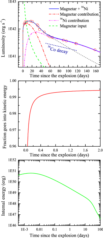
Figure 1.— The light curve (top), the fraction of magnetar rotational energy deposited as the kinetic energy of SN 1997ef (middle), and the internal energy of the SN (bottom). In the top panel the solid line is the light curve produced by taking account for the contribution from both magnetar and ⁵⁶Ni, while the dot-dashed line is the light curve by setting the mass of ⁵⁶Ni zero while other parameters are the same as that of the solid line. The dot-dot-dashed line is the difference between solid line and the dot-dashed line. The dark short-dashed line is the light curve with $\kappa_{\gamma,\mathrm{decay}}=0.027\mathord{\thinspace\rm cm}^{2}\mathord{\thinspace\rm g}^{-1}$. Please note that the abscissa time scales in these panels are quite different and the last panel is in logarithmic scale. The data points are taken from Iwamoto et al. (2000).

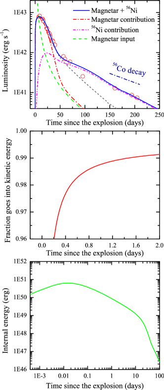
Figure 2.— The same as Figure 1 but for SN 2007ru. The data points are taken from Sahu et al. (2009).

Figures 1 and 2 show the results of the analytical model with best-fit parameters listed in Table 1. In these fits, we adopt the widely used value $\kappa=0.1\mathord{\thinspace\rm cm}^{2}\mathord{\thinspace\rm g}^{-1}$ so that there are effectively four free parameters in this model. From Figures 1 and 2 it is clear that the contribution to the light curves from magnetars at late times is negligible.

Table 1Best-fit parameters for SNe 1997ef and 2007ru. In these fits, we fix $\kappa=0.1\mathord{\thinspace\rm cm}^{2}\mathord{\thinspace\rm g}^{-1}$.

SN	$M_{\mathrm{ej}}$	$M_{\mathrm{Ni}}$	$B_{p}$	$P_{0}$
	$\left(M_{\odot}\right)$	$\left(M_{\odot}\right)$	$\left(10^{16}\mathord{\thinspace\rm G}\right)$	$\left(\mathord{\thinspace\rm ms}\right)$
SN 1997ef	$5.9$	$0.056$	$1.24$	$2.25$
SN 2007ru	$4.43$	$0.061$	$0.62$	$2.30$

Comparison of Figure 1 with the ⁵⁶Ni-powered light curve (Iwamoto et al., 2000) immediately shows the superior fitting quality of the light curve in Figure 1. It is worthy of mentioning that the above analytical model, as a direct extension of the Arnett model (Arnett, 1982), is quite good at reproducing the light curve of a purely ⁵⁶Ni-powered SN (Arnett & Fu, 1989). When applying the pure ⁵⁶Ni model to SNe Ic-BL, the mass of ⁵⁶Ni is determined by the peak luminosity of the SN. But the ⁵⁶Co tail modeling usually requires a much lower mass of ⁵⁶Ni. Hence an inconsistency appears. In other words, the poor fitting quality of the pure ⁵⁶Ni model is intrinsic for SNe Ic-BL.

Figures 1 and 2 indicate that the (assumed) magnetars contribute dominantly to the early peaks of the light curves. This is the key that the actually needed ⁵⁶Ni, $M_{\mathrm{Ni}}\sim 0.06M_{\odot}$ for both SNe 1997ef and 2007ru, is much lower than a pure ⁵⁶Ni model. It is also evident from these figures that the late-time luminosities of these SNe dominantly come from the decay energy of ⁵⁶Ni and ⁵⁶Co.

Table 1 shows that the ejecta masses $M_{\mathrm{ej}}$ are different from that given by the pure-⁵⁶Ni model, which favors the ejecta masses $M_{\mathrm{ej}}=7.6M_{\odot}$ and $M_{\mathrm{ej}}=1.3M_{\odot}$ for SNe 1997ef (Iwamoto et al., 2000) and 2007ru (Sahu et al., 2009), respectively. This difference is mainly because in this model the light curve peak is not caused by ⁵⁶Ni. It can be checked that the values given in Table 1 is consistent with Equation $\left(\ref{eq:tau_m-SN}\right)$ if we realize that $\tau_{m}$ should be set equal to the rising time of ⁵⁶Co contribution in Figures 1 and 2. In these figures the asymptotic expansion velocities are set to $1.1\times 10^{4}\mathord{\thinspace\rm km}\mathord{\thinspace\rm s}^{-1}$ and $1.3\times 10^{4}\mathord{\thinspace\rm km}\mathord{\thinspace\rm s}^{-1}$ for SNe 1997ef and 2007ru, respectively. It is curious that the derived value $M_{\mathrm{ej}}=7.6M_{\odot}$ by Iwamoto et al. (2000) for SN 1997ef is even larger than the value given in this work in spite of the fact that the rising time in the pure-⁵⁶Ni model is shorter than the rising time of ⁵⁶Co contribution in Figure 1. We note that the two models in Iwamoto et al. (2000), i.e. CO60 and CO100, are almost identical in fitting the light curve of SN 1997ef, but give different values of ejecta mass, $M_{\mathrm{ej}}=4.6M_{\odot}$ and $M_{\mathrm{ej}}=7.6M_{\odot}$, respectively. One can check that $M_{\mathrm{ej}}=4.6M_{\odot}$ is consistent with the light curve rising time if the optical opacity is taken as $\kappa=0.1\mathord{\thinspace\rm cm}^{2}\mathord{\thinspace\rm g}^{-1}$. This may indicate the uncertainty in the numerical modeling by Iwamoto et al. (2000).

The ⁵⁶Ni yield determined in the pure-⁵⁶Ni model is $M_{\mathrm{Ni}}=0.15M_{\odot}$ and $M_{\mathrm{Ni}}=0.4M_{\odot}$ for these two SNe, respectively. As we said, the yield $M_{\mathrm{Ni}}=0.4M_{\odot}$ is hardly expected by the magnetar-driven shock ⁵⁶Ni synthesis (Nishimura et al., 2015; Suwa & Tominaga, 2015). In addition, what makes the pure-⁵⁶Ni model for SN 2007ru more or less unrealistic is the derived ratio $M_{\mathrm{Ni}}/M_{\mathrm{ej}}\simeq 0.3$, in tension with the theoretical expectation, which is predicted to be hardly larger than 0.2 (Umeda & Nomoto, 2008).

In the middle panels of Figures 1 and 2 we show the fraction of magnetar rotational energy deposited as the kinetic energy of the SN ejecta. From these figures it is clear that most ($>99\%$) of the rotational energy of the magnetars deposits as the kinetic energy of the SN ejecta and only $<1\%$ of the rotational energy deposits to heat the ejecta, which is in accord with the expectation (Wang et al., 2016b).

To figure out why only $\sim 1\%$ of the rotational energy is enough to heat the SNe Ic-BL to the observed luminosity, it is beneficial to compare the rotational energy of the magnetars

$$E_{p}=2\times 10^{52}I_{45}P_{0,-3}^{-2}\mathord{\thinspace\rm erg}$$ (12)

with the decay energy of ⁵⁶Ni and ⁵⁶Co

$$E_{\mathrm{decay}}=1.88\times 10^{50}\frac{M_{\mathrm{Ni}}}{M_{\odot}}\mathord{\thinspace\rm erg}.$$ (13)

Assuming that a fraction $\eta_{E}$ of the rotational energy of the magnetar $E_{p}$ is converted to the thermal energy of the SN, then the deposited thermal energy by the magnetar is equivalent to ⁵⁶Ni of mass

$$M_{\mathrm{Ni}}=1.047I_{45}P_{0,-3}^{-2}\eta_{E,-2}M_{\odot},$$ (14)

where $\eta_{E}=0.01\eta_{E,-2}$. Because the needed masses of ⁵⁶Ni by the previous analysis are $0.2-0.5M_{\odot}$, it is evident that the typical initial rotational period of the magnetars that powers the SNe Ic-BL is $P_{0}\simeq 2\mathord{\thinspace\rm ms}$, in agreement with the values given in Table 1.

The bottom panels of Figures 1 and 2 show the evolution of the SN internal energy with initial value $10^{50}\mathord{\thinspace\rm erg}$. As expected, the SN internal energy increases only slightly despite the tremendous energy injection rate $\gtrsim 10^{50}\mathord{\thinspace\rm erg}\mathord{\thinspace\rm s}^{-1}$ during the spin-down timescale $\sim 10^{-3}\mathord{\thinspace\rm days}$. This is just why the SNe Ic-BL powered by a rapidly spinning-down magnetar can gain the formidable kinetic energy $\sim 10^{52}\mathord{\thinspace\rm erg}$.

With the parameters in Table 1, it seems difficult to understand how a magnetar with spin-down timescale as short as $\sim 10^{-3}\mathord{\thinspace\rm days}$ can power an SN lasting for $\sim 20\mathord{\thinspace\rm days}$. This can be most easily understood by evaluating how much magnetar rotational energy is left at the light curve peak time $t_{\mathrm{pk}}$. Because $t_{\mathrm{pk}}\gg T_{\mathrm{sd}}$, the energy left at time $t_{\mathrm{pk}}$ is

$$E=E_{0}\left(1+\frac{t_{\mathrm{pk}}}{T_{\mathrm{sd}}}\right)^{-1}\sim 10^{48}\mathord{\thinspace\rm erg}E_{0,52}t_{\mathrm{pk},6}^{-1}T_{\mathrm{sd},2}.$$ (15)

This energy is just enough for most SNe Ic-BL with peak luminosity $\sim 10^{42}\mathord{\thinspace\rm erg}\mathord{\thinspace\rm s}^{-1}$ lasting for $\sim 10\mathord{\thinspace\rm days}$.

In the analytical model (Wang et al., 2016b) it is expected that the magnetic dipole field of the (assumed) magnetars that powers SNe Ic-BL is much stronger than that powers SLSNe. This is evident from Table 1 that the best-fit magnetic dipole field of the magnetar is $B_{p}\sim 10^{16}\mathord{\thinspace\rm G}$, whereas the magnetic field in the case of SLSNe is typically $B_{p}\sim 10^{14}\mathord{\thinspace\rm G}$.

Finally, because of the high magnetic field strength $B_{p}\sim 10^{16}\mathord{\thinspace\rm G}$ and the rapid spinning of the magnetar $P_{0}\simeq 2\mathord{\thinspace\rm ms}$, the ⁵⁶Ni with mass as low as $0.06M_{\odot}$ can be synthesized by the magnetar model (Suwa & Tominaga, 2015). It is clear from above analyses that a self-consistent magnetar model for the SNe Ic-BL is established.

4. Discussion

Since their discovery, SNe Ic-BL pose an immediate challenge to the classical SN light curve modeling because the later failed to simultaneously reproduce the light curve around peak and the late-time linear decline. As a plausible attempt, Maeda et al. (2003) proposed a two-component model for SNe Ic-BL in which the bright peak is produced by the fast-moving outer component while the linear tail is attributed to the slower dense inner component. Because the two-component model and the model presented here both assume that the linear tail of the SNe Ic-BL light curve can be attributed to ⁵⁶Co decay, it would be beneficial to compare the ⁵⁶Ni mass inferred here with the inner component ⁵⁶Ni mass inferred in the two-component model. For SN 1997ef, Maeda et al. (2003) gave the ⁵⁶Ni mass of the inner component $M_{\mathrm{Ni,inner}}=0.08M_{\odot}$, which is close to our determination taking into account the different value of $\kappa$ adopted in these two works. We also note that for the GRB-associated SN 1998bw, Maeda et al. (2003) found $M_{\mathrm{Ni,inner}}=0.1M_{\odot}$, which is much smaller than the usually assumed value $M_{\mathrm{Ni}}\simeq 0.5M_{\odot}$. This justifies our finding that the ⁵⁶Ni mass for the tail modeling is usually much smaller than the peak modeling.

Our results have immediate stimulations for further research. First, although here we have studied the SNe Ic-BL not associated with GRBs, the main conclusion can be equally applied to GRB-SNe. It is usually believed that the central engine of GRBs are black holes (Popham et al., 1999; Narayan et al., 2001; Kohri & Mineshige, 2002; Liu et al., 2007; Song et al., 2016) or magnetars (Usov, 1992; Dai & Lu, 1998a, b; Zhang & Dai, 2008, 2009, 2010; Giacomazzo & Perna, 2013; Giacomazzo et al., 2015). However, since it is currently infeasible to identify the GRB central engine directly because of the cosmological distance scales of GRBs (Kumar & Zhang, 2015), the researchers instead pursue indirect signatures of black holes (Geng et al., 2013; Wu et al., 2013; Yu et al., 2015) and magnetars (Dai et al., 2006; Gao et al., 2013; Wang & Dai, 2013; Zhang, 2013; Yu et al., 2013; Metzger & Piro, 2014; Wang et al., 2015a, 2016a; Li & Yu, 2016; Liu et al., 2016) that powers the energetic GRBs. Growing indirect observational evidence suggests that magnetars could act as the central engine of both LGRBs and SGRBs (Dai et al., 2006; Rowlinson et al., 2010, 2013; Dai & Liu, 2012; Wang & Dai, 2013; Wu et al., 2014; Gao et al., 2015; Greiner et al., 2015). However, because of the high mass of ⁵⁶Ni needed to heat the GRB-SNe, magnetars are doubted as the candidate central engine of GRBs. With our demonstration that this high mass of ⁵⁶Ni is actually not the case, such a concern is removed.

Second, it is still debated how the jet is launched by a rapidly rotating magnetar. Comparison of SLSNe and SN Ic-BL may have some implications for this open issue. Observation shows little evidence of jet associated with SLSNe (Leloudas et al., 2015), while some SNe Ic-BL are accompanied by GRB jets. Even for those SNe Ic-BL not associated with GRBs, jets or aspheric expansion are frequently observed. Because the initial rotational periods of the magnetars that power SLSNe and SNe Ic-BL are similar, we hypothesize that the magnetic field of the magnetar might be essential for the jet launch given the fact that the magnetic field of magnetar that powers SNe Ic-BL is much stronger than that powers SLSNe. This hypothesis relies on future numerical simulations. We note, however, that Greiner et al. (2015) found the magnetic dipole field of the (assumed) magnetar powering GRB111209A/SN2011kl to be only $\left(6-9\right)\times 10^{14}\mathord{\thinspace\rm G}$, close to that powering SLSNe. This may indicate that strong magnetic field is not a necessary condition for jet launch. Nevertheless, the contamination by GRB afterglow and host galaxy background makes the GRB-SNe light curves poorly sampled and parameter degeneracy could bias the fitting values, e.g. the magnetic dipole field $B_{p}$ and the ⁵⁶Ni masses.

Third, we find that the typical magnetic field of the (assumed) magnetars that powers SNe Ic-BL is $10^{16}\mathord{\thinspace\rm G}$, which is two orders of magnitude stronger than the field of the magnetars that powers SLSNe, despite the fact that they are both millisecond magnetars and are all formed during the core collapse of massive progenitors. This implies that the magnetic amplification mechanisms (Mösta et al., 2015) could be quite different. This calls for more elaborated numerical simulations that take into account more microphysical processes. The dipole field as strong as $10^{16}\mathord{\thinspace\rm G}$ is rare but achievable in theoretical aspects. It is expected that the collapse of the iron core of the supernova progenitor first results in a proto-neutron star (PNS). The differential rotation of PNS could amplify the toroidal field to $\sim 10^{16}\mathord{\thinspace\rm G}$ and above (Wheeler et al., 2000). Several magnetic field amplification mechanisms could operate, including the linear amplification (Dai et al., 2006), $\alpha$-$\Omega$ dynamo (Duncan & Thompson, 1992; Thompson & Duncan, 1993), and magnetorotational instability (Balbus & Hawley, 1998). The toroidal field could be amplified to $\sim 10^{17}\mathord{\thinspace\rm G}$ before the buoyancy effect takes it to emerge from the neutron star surface (Kluźniak & Ruderman, 1998; Dai et al., 2006). It is possible that the emerged dipole field could be as strong as $\sim 10^{16}\mathord{\thinspace\rm G}$.

In addition, because the bona fide ⁵⁶Ni yield is much lower than previously thought, the kinetic energy-⁵⁶Ni mass relation (Mazzali et al., 2013) should be substantially revised. By doing so some new insights could be unveiled.

References

- Arnett (1980) Arnett, W. D. 1980, ApJ, 237, 541
- Arnett (1982) Arnett, W. D. 1982, ApJ, 253, 785
- Arnett & Fu (1989) Arnett, W. D., & Fu, A. 1989, ApJ, 340, 396
- Balbus & Hawley (1998) Balbus, S. A., & Hawley, J. F. 1998, RvMP, 70, 1
- Bethe (1990) Bethe, H. A. 1990, RvMP, 62, 801
- Cano et al. (2016a) Cano, Z., Johansson Andreas, K. G., & Maeda, K. 2016a, MNRAS, 457, 2761
- Cano et al. (2016b) Cano, Z., Wang, S. Q., Dai, Z. G., & Wu, X. F. 2016b, arXiv:1604.03549
- Chatzopoulos et al. (2012) Chatzopoulos, E., Wheeler, J. C., & Vinko, J. 2012, ApJ, 746, 121
- Chatzopoulos et al. (2013) Chatzopoulos, E., Wheeler, J. C., Vinko, J., et al. 2013, ApJ, 773, 76
- Chen et al. (2015) Chen, T. W., Smartt, S. J., Jerkstrand, A., et al. 2015, MNRAS, 452, 1567
- Dai & Liu (2012) Dai, Z. G. & Liu, R. Y. 2012, ApJ, 759, 58
- Dai & Lu (1998a) Dai, Z. G., & Lu, T. 1998a, A&A, 333, L87
- Dai & Lu (1998b) Dai, Z. G., & Lu, T. 1998b, PhRvL, 81, 4301
- Dai et al. (2016) Dai, Z. G., Wang, S. Q., Wang, J. S., Wang, L. J., & Yu, Y. W. 2016, ApJ, 817, 132
- Dai et al. (2006) Dai, Z. G., Wang, X. Y., Wu, X. F. & Zhang, B. 2006, Sci, 311, 1127
- Duncan & Thompson (1992) Duncan, R. C., & Thompson, C. 1992, ApJL, 392, L9
- Filippenko (1997) Filippenko, A. V. 1997, ARA&A, 35, 309
- Gal-Yam et al. (2009) Gal-Yam, A., Mazzali, P., Ofek, E. O., et al. 2009, Natur, 462, 624
- Gao et al. (2015) Gao, H., Ding, X., Wu, X. F., Dai, Z. G., & Zhang, B. 2015, ApJ, 807, 163
- Gao et al. (2013) Gao, H., Ding, X., Wu, X. F., Zhang, B., & Dai, Z. G. 2013, ApJ, 771, 86
- Geng et al. (2013) Geng, J. J., Wu, X. F., Huang, Y. F., & Yu, Y. B. 2013, ApJ, 779, 28
- Giacomazzo & Perna (2013) Giacomazzo, B., & Perna, R. 2013, ApJL, 771, L26
- Giacomazzo et al. (2015) Giacomazzo, B., Zrake, J., Duffell, P. C., et al. 2015, ApJ, 809, 39
- Greiner et al. (2015) Greiner, J., Mazzali, P. A., Kann, D. A., et al. 2015, Natur, 523, 189
- Inserra et al. (2013) Inserra, C., Smartt, S. J., Jerkstrand, A., et al. 2013, ApJ, 770, 128
- Iwamoto et al. (2000) Iwamoto, K., Nakamura, T., Nomoto, K., et al. 2000, ApJ, 534, 660
- Janka (2012) Janka, H-T. 2012, ARNPS, 62, 407
- Kasen & Bildsten (2010) Kasen, D., & Bildsten, L. 2010, ApJ, 717, 245
- Kashiyama et al. (2016) Kashiyama, K., Murase, K., Bartos, I., et al. 2016, ApJ, 818, 94
- Kluźniak & Ruderman (1998) Kluźniak, W., & Ruderman, M. 1998, ApJL, 505, L113
- Kohri & Mineshige (2002) Kohri, K., & Mineshige, S. 2002, ApJ, 577, 311
- Kumar & Zhang (2015) Kumar, P., & Zhang, B. 2015, PhR, 561, 1
- Leloudas et al. (2015) Leloudas, G., Patat, F., Maund, J. R., et al. 2015, ApJL, 815, L10
- Li & Yu (2016) Li, S. Z., & Yu, Y. W. 2016, ApJ, 819, 120
- Liu et al. (2016) Liu, L. D., Wang, L. J., & Dai, Z. G. 2016, A&A, 592, A92
- Liu et al. (2007) Liu, T., Gu, W. M., Xue, L., & Lu, J. F. 2007, ApJ, 661, 1025
- Maeda et al. (2003) Maeda, K., Mazzali, P. A., Deng, J. S., et al. 2003, ApJ, 593, 931
- Mazzali et al. (2014) Mazzali, P. A., McFadyen, A. I., Woosley, S. E., Pian, E., & Tanaka, M. 2014, MNRAS, 443, 67
- Mazzali et al. (2013) Mazzali, P. A., Walker, E. S., Pian, E., et al. 2013, MNRAS, 432, 2463
- Metzger et al. (2015) Metzger, B. D., Margalit, B., Kasen, D., Quataert, E. 2015, MNRAS, 454, 3311
- Metzger & Piro (2014) Metzger, B. D., & Piro, A. L. 2014, MNRAS, 439, 3916
- Milisavljevic et al. (2015) Milisavljevic, D., Margutti, R., Parrent, J. T., et al. 2015, ApJ, 799, 51
- Mösta et al. (2015) Mösta, P., Ott, C. D., Radice, D., et al. 2015, Natur, 528, 376
- Narayan et al. (2001) Narayan, R., Piran, T., & Kumar, P. 2001, ApJ, 557, 949
- Nicholl et al. (2014) Nicholl, M., Smartt, S. J., Jerkstrand, A., et al. 2014, MNRAS, 444, 2096
- Nishimura et al. (2015) Nishimura, N., Takiwaki, T., & Thielemann, F.-K. 2015, ApJ, 810, 109
- Pignata et al. (2011) Pignata, G., Stritzinger, M., Soderberg, A., et al. 2011, ApJ, 728, 14
- Popham et al. (1999) Popham, R., Woosley, S. E., & Fryer, C. 1999, ApJ, 518, 356
- Rowlinson et al. (2013) Rowlinson, A., O’Brien, P. T., Metzger, B. D., et al. 2013, MNRAS, 430, 1061
- Rowlinson et al. (2010) Rowlinson, A., O’Brien, P. T., Tanvir, N. R., et al. 2010, MNRAS, 409, 531
- Sahu et al. (2009) Sahu, D. K., Tanaka, M., Anupama, G. C., et al. 2009, ApJ, 697, 676
- Song et al. (2016) Song, C. Y., Liu, T., Gu, W. M., Tian, J. X. 2016, MNRAS, 458, 1921
- Suwa & Tominaga (2015) Suwa, Y., & Tominaga, N. 2015, MNRAS, 451, 282
- Thompson & Duncan (1993) Thompson, C., & Duncan, R. C. 1993, ApJ, 408, 194
- Thompson et al. (2004) Thompson, T. A., Chang, P., & Quataert, E. 2004, ApJ, 611, 380
- Umeda & Nomoto (2008) Umeda, H., & Nomoto, K. 2008, ApJ, 673, 1014
- Usov (1992) Usov, V. V. 1992, Natur, 357, 472
- Wang & Dai (2013) Wang, L. J., & Dai, Z. G. 2013, ApJL, 774, L33
- Wang et al. (2015a) Wang, L. J., Dai, Z. G., & Yu, Y. W. 2015a, ApJ, 800, 79
- Wang et al. (2016a) Wang, L. J., Dai, Z. G., Liu, L. D., & Wu, X. F. 2016a, ApJ, 823, 15
- Wang et al. (2016b) Wang, L. J., Wang, S. Q., Dai, Z. G., et al. 2016b, ApJ, 821, 22
- Wang et al. (2016c) Wang, S. Q., Liu, L. D., Dai, Z. G., Wang, L. J., & Wu, X. F. 2016c, ApJ, 828, 87
- Wang et al. (2015b) Wang, S. Q., Wang, L. J., Dai, Z. G., & Wu, X. F. 2015b, ApJ, 799, 107
- Wang et al. (2015c) Wang, S. Q., Wang, L. J., Dai, Z. G., & Wu, X. F. 2015c, ApJ, 807, 147
- Wheeler et al. (2000) Wheeler, J. C., Yi, I., Höflich, P., & Wang, L. 2000, ApJ, 537, 810
- Woosley (2010) Woosley, S. E. 2010, ApJL, 719, L204
- Woosley & Bloom (2006) Woosley, S. E. & Bloom, J. S. 2006, ARA&A, 44, 507
- Woosley et al. (2002) Woosley, S. E., Heger, A., & Weaver, T. A. 2002, RvMP, 74 , 1015
- Wu et al. (2013) Wu, X. F., Hou, S. J., & Lei, W. H. 2013, ApJL, 767, L36
- Wu et al. (2014) Wu X. F., Gao H., Ding X., Zhang B., Dai Z. G., Wei J. Y., 2014, ApJL, 781, L10
- Yu et al. (2015) Yu, Y. B., Wu, X. F., Huang, Y. F., et al. 2015, MNRAS, 446, 3642
- Yu et al. (2013) Yu, Y. W., Zhang, B., & Gao, H. 2013, ApJL, 776, L40
- Zhang (2013) Zhang, B. 2013, ApJL, 763, L22
- Zhang & Dai (2008) Zhang, D., & Dai, Z. G. 2008, ApJ, 683, 329
- Zhang & Dai (2009) Zhang, D., & Dai, Z. G. 2009, ApJ, 703, 461
- Zhang & Dai (2010) Zhang, D., & Dai, Z. G. 2010, ApJ, 718, 841