Regularization for supervised learning via the “hubNet” procedure

Abstract

We propose a new method for supervised learning. The hubNet procedure fits a hub-based graphical model to the predictors, to estimate the amount of “connection” that each predictor has with other predictors. This yields a set of predictor weights that are then used in a regularized regression such as the lasso or elastic net. The resulting procedure is easy to implement, can sometimes yields higher prediction accuracy that the lasso, and can give insights into the underlying structure of the predictors. HubNet can also be generalized seamlessly to other supervised problems such as regularized logistic regression (and other GLMs), Cox’s proportional hazards model, and nonlinear procedures such as random forests and boosting. We prove some recovery results under a specialized model and illustrate the method on real and simulated data.

1 Introduction

We consider the usual linear regression model: Given $n$ realizations of $p$ predictors ${\bf X}=\{x_{ij}\}$ for $i=1,2,\ldots,n$ and $j=1,2,\ldots,p$, the response $Y=(y_{1},\ldots,y_{n})$ is modeled as

$$y_{i}=\beta_{0}+\sum_{j}x_{ij}\beta_{j}+\epsilon_{i}$$ (1)

with $\epsilon\sim(0,\sigma^{2})$. The ordinary least squares (OLS) estimates of $\beta_{j}$ are obtained by minimizing the residual sum of squares. There has been much work on regularized estimators that offer an advantage over the OLS estimates, both in terms of accuracy of prediction on future data and interpretation of the fitted model. One major focus has been on the lasso (Tibshirani, 1996), which minimizes

$$J(\beta_{0},\beta)=\frac{1}{2}\|Y-\beta_{0}-{\bf X}\beta\|_{2}^{2}+\lambda\|\beta\|_{1}$$ (2)

where $\beta=(\beta_{1},\ldots,\beta_{p})$, and the tuning parameter $\lambda\geq 0$ controls the sparsity of the final model. This parameter is often selected by cross-validation. The objective function $J(\beta_{0},\beta)$ is convex, which means that the solutions can be found efficiently even for very large $n$ and $p$, in contrast to combinatorial methods like best subset selection. A body of mathematical work shows that under certain conditions, the lasso often will provide good recovery of the underlying true model and will produce predictions that are mean-square consistent (Knight and Fu, 2000; Meinshausen and Bühlmann, 2006; Zhao and Yu, 2006; Bunea et al., 2007; Zhang and Huang, 2008; Meinshausen and Yu, 2009; Bickel et al., 2009; Wainwright, 2009). The elastic net of Zou and Hastie (2005) generalizes the lasso by adding an $\ell_{2}$ penalty,

$$\frac{1}{2}\|Y-\beta_{0}-{\bf X}\beta\|_{2}^{2}+\lambda(\alpha\|\beta\|_{1}+(1-\alpha)\|\beta\|_{2}^{2}),$$ (3)

where $\alpha\in[0,1]$ is a second tuning parameter. This approach sometimes yields lower prediction error than the lasso, especially in settings with highly correlated predictors.

Zou (2006) introduced the adaptive lasso, which minimizes

$$\frac{1}{2}\|Y-\beta_{0}-{\bf X}\beta\|_{2}^{2}+\lambda\sum_{j}w_{j}|\beta_{j}|$$ (4)

for feature weights $w_{j}$. The feature weights can be chosen in various ways: For example, when $n>p$, we can first compute the OLS estimates $\hat{\beta}_{j}$ and then set $w_{j}=1/|\hat{\beta}_{j}|$. For $p>n$, we can set $w_{j}$ by first computing univariate regression coefficients (Huang et al., 2008). Other similar “two-step” procedures include variants of the non-negative garrote (Breiman, 1995; Yuan and Lin, 2007) and the adaptive elastic net (Zou and Zhang, 2009). We have found that one less than ideal property of the adaptive lasso is that there seems to be no underlying generative model that leads to its feature weighting. Perhaps as a result, it is difficult even to simulate a dataset that shows substantial gains for the method, relative to the usual lasso.

In this paper, we provide a new perspective by choosing weights in the adaptive lasso in an unsupervised manner. All of the above two-step procedures select weights by computing an initial estimate $\hat{\beta}$ using the response $Y$. We instead propose to use the partial correlations of the features in ${\bf X}$ to select good weights. We postulate a conceptual model in which there is a core subset $S$ of “hub” features that explains both the other features and $Y$. For example, each member of $S$ might be the RNA or protein expression of a “driver” gene in a pathway which simultaneously influences other gene expressions and the phenotype under study. Our method, called hubNet, fits an (unsupervised) graphical model to the features in a way that tries to discover these “hubs”. These features are then given higher weight in the adaptive lasso. The hubNet procedure can sometimes yield lower prediction error and better support recovery than the lasso, and the discovered hubs can provide insight on the underlying structure of the data.

This paper is organized as follows. In Section 2 we introduce our underlying model and the hubNet procedure. Simulation studies are presented in Section 3, while Section 4 examines applications to real datasets. Some theoretical results on the recovery of the underlying model are given in Section 5. Further topics are discussed in Section 6, such as extensions to random forests and post-selection inference. Section 7 compares our method of identifying hubs with an alternative approach.

1.1 Illustrative example: Olive oil data

The data for this example, from Forina et al. (1983), consists of measurements of 8 fatty acid concentrations for 572 olive oils, with each olive oil classified into one of two geographic regions. The goal is to determine the geographic region based on these 8 predictors. We randomly divided the data into training and test sets of equal size. The predictors are:

1. Palmitic Acid

2. Palmitoleic Acid

3. Stearic Acid

4. Oleic Acid

5. Linoleic Acid

6. Linolenic Acid

7. Arachidic Acid

8. Eicosenoic Acid

Results from hubNet and lasso-regularized logistic regression are given in Figure 1 with details in the caption. (Extension of hubNet to logistic regression is straightforward and discussed in Section 2.4.) HubNet focuses on just two predictors—2 and 4, which have apparent connections to the other six. In the process, it yields a more parsimonious model than the lasso, with perhaps a lower CV and test error.

Figure 1: Results for olive oil data. Top left panel shows coefficients from lasso (black), hub weights (broken green line) and resulting coefficients from hubNet (solid green). hubNet chooses predictors 2 (palmitoleic acid) and 4 (oleic acid), having connections to other predictors as depicted in the top right panel. The boldness of the link corresponds to the strength of the association. The bottom panels show the cross-validation and test error for the lasso and hubNet.

2 The hubNet procedure

Let $Y=(y_{1},\ldots,y_{n})$ and let ${\bf X}=\{x_{ij}\}$ be the $n\times p$ matrix of features. Define the core set $S$ to be a subset of $\{1,2,\ldots p\}$, with corresponding feature matrix ${\bf X}_{S}$. Our proposal is based on the following model:

$$Y = \beta_{0}+{\bf X}_{S}\beta+\epsilon$$ (5)

$$X_{j} = {\bf X}_{S}\Gamma_{j}+\epsilon_{j},\;\;j\notin S$$ (6)

where each $\Gamma_{j}$ is an $s\times 1$ coefficient vector. This model postulates that the outcome $Y$ is a function of an (unknown) core set of predictors $S$, and that the predictors not in $S$ are also a function of this same core set.

If this model holds, even approximately, then we can examine the partial correlations among the features to determine the features more likely to belong to this core set $S$, and hence do a better job of predicting $Y$. Following this logic, our proposal for estimating $\beta$ in (5) consists of three steps:

The hubNet procedure

1. Fit a model of the form ${\bf X}\approx{\bf X}{\bf B}$ with ${\bf B}_{ii}=0$ using the “edge-out” procedure detailed in Section 2.1 below. Note that $\Gamma_{j}$ in the generating model (6) correspond to coefficients of ${\bf B}$ in rows $S$ and columns $S^{C}$.

2. Let $s_{j}=\sum_{j}|\hat{\bf B}_{ij}|,j=1,2,\ldots,p$, and construct feature weights

   $$w_{j}=1/s_{j}\,.$$ (7)

3. Fit the adaptive lasso using predictors and feature weights $w_{j}$ (e.g., using $w_{j}$ as “penalty factors” in the glmnet R package.) [If $s_{j}=0$, then $w_{j}=\infty$ and $X_{j}$ is not used.]

The hubNet procedure has a number of attractive features:

(a) The construction of weights is completely unsupervised, separating it from the fitting of the response model in step 3. Thus for example, cross-validation can be applied in step 3 and we can use cross-validation to choose between hubNet and lasso for a given problem. In addition, tools for post-selection inference for the lasso can be directly applied.

(b) The supervised fitting in step 3 is simply a lasso (or elastic net) with feature weights, hence fast off-the-shelf solvers can be used.

(c) Examination of the estimated hub structure for the chosen predictors can shed light on the structure of the final model.

(d) The procedure can be directly applied to generalized regression settings, such as generalized linear models and the proportional hazards model for survival data, using an appropriate method in step 3.

The challenging task of the hubNet procedure is step 1. For this, one might use the graphical lasso, which produces a sparse estimate of the inverse covariance matrix, corresponding to an edge-sparse feature graph. But we would like an estimate that encourages the appearance of hub nodes, i.e., features having many non-zero partial correlations with other features. These hub nodes then represent our estimate of the core set $S$. Tan et al. (2014) propose a method called hglasso for learning graphical models with hubs, which produces a proper (non-negative definite) estimate of the inverse covariance matrix. Their procedure uses an ADMM algorithm having computational complexity $O(p^{3})$ per iteration, which in our experience is too slow for problems with $p=1000$ or greater. We instead use the “edge-out” method of Friedman et al. (2010), which has complexity $O(\min(np^{2}+snp,sp^{2}))$ per iteration. A comparison of these methods is presented in Section 7.

2.1 The edge-out procedure

To estimate ${\bf B}$ in step 1 of the hubNet procedure, we use the edge-out estimator

$$\hat{{\bf B}}_{eo}=\operatorname*{arg\,min}_{{\bf B}\in{}^{p\times p}:\,{\bf B}_{ii}=0\,\forall i}\frac{1}{2}\|{\bf X}-{\bf X}{\bf B}\|^{2}_{F}+\theta\cdot\left(\gamma\|{\bf B}_{i,.}||_{1}+(1-\gamma)\sqrt{p-1}\sum_{i=1}^{p}\|{\bf B}_{i,.}\|_{2}\right).$$ (8)

Here, $\theta,\gamma>0$ are tuning parameters, $\|\cdot\|_{F}$ denotes the Frobenius norm, and ${\bf B}_{i,.}$ denotes the $i$th row of ${\bf B}$.

By constraining the diagonal entries of ${\bf B}$ to 0, the edge-out estimator simultaneously regresses each feature onto the remaining features of ${\bf X}$. The procedure applies a combined $\ell_{1}/\ell_{2}$ penalty on the regression coefficients, where the $\ell_{2}$ penalty encourages zeroing-out of entire rows of ${\bf B}$ and the $\ell_{1}$ penalty encourages additional sparsity in the non-zero rows. (The original hubNet proposal of Friedman et al. (2010) used only the $\ell_{2}$ penalty.) The estimate $\hat{{\bf B}}_{eo}$ is not symmetric. We expect the “hub” features in the core set $S$ to correspond to the rows of ${\bf B}$ having many non-zero entries, and hence the row sums should give higher weight to these features in steps 2 and 3. Our procedure for minimization of the edge-out objective is outlined in Appendix A.

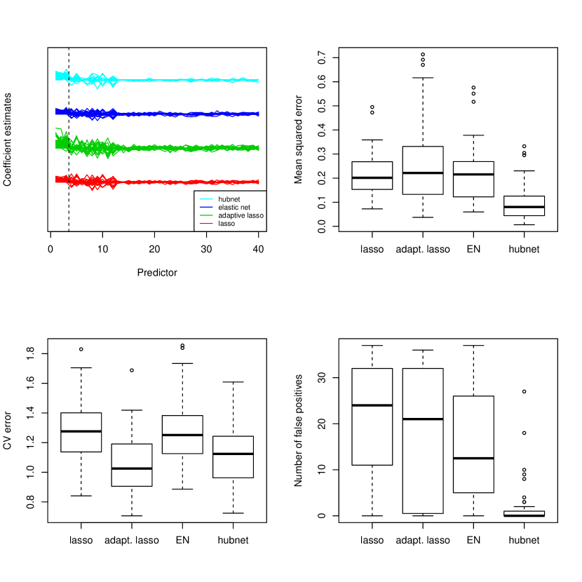
Figure 2: Estimates from 20 simulations from underlying hub model; $n=60,p=40$, and first 3 predictors are hub predictors and contain the signal. The top left panel shows the estimated coefficients over 20 realizations. The top right panel displays the mean-squared test error with the tuning parameter chosen by cross-validation for each method. The bottom left panel shows the minimum CV error for each realization: note that the adaptive lasso CV error is not a valid estimate of error since the weights are estimated in a supervised manner. The bottom right panel shows the number of false positive predictors, in the smallest model where in the procedure has “screened”, i.e. contains all of the true predictors.

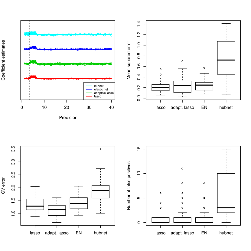
Figure 3: Estimates from 20 simulations from underlying hub model; $n=60,p=40$, first 3 predictors are hub predictors, but signal is a function of predictors 4 to 6. See previous figure caption for details of panels.

2.2 Choosing tuning parameters for edge-out

We have two proposals for setting the tuning parameter $\theta$ in the edge-out method. The first is $K$-fold cross-validation, applied to the objective function $\frac{1}{2}||{\bf X}-{\bf X}{\bf B}||^{2}_{F}$. The second uses a form of generalized cross validation

$$\operatorname{GCV}(\hat{{\bf X}})=\frac{||{\bf X}-\hat{{\bf X}}||^{2}_{2}}{np-{\rm df}(\hat{{\bf X}})}.$$

If there is only an $\ell_{1}$ penalty, we use for ${\rm df}(\hat{{\bf X}})$ the number of non-zero entries $|\hat{{\bf B}}|_{0}$. If there is also an $\ell_{2}$ penalty, we propose the following adjustment based on our updating formula:

$${\rm df}(\hat{{\bf X}})=\sum_{i=1}^{p}\frac{\|\hat{{\bf B}}_{i,.}||_{2}}{\|\hat{{\bf B}}_{i,.}\|_{2}+\theta(1-\gamma)\sqrt{p-1}}\|\hat{{\bf B}}_{i,.}\|_{0}.$$

Note that this is not an exact formula for degrees of freedom, but rather a rough estimate.

2.3 Simulated data example.

Figure 2 shows hubNet applied to a simulated data example. Here $n=60$, $p=40$, and the first 3 predictors are the core set, explaining both $Y$ and the remaining 37 predictors. The estimated coefficients and various error rates of hubNet over 20 realizations are shown, in comparison to the elastic net, adaptive lasso, and lasso. We see that hubNet does a much better job at recovering the true coefficients, which in turn leads to substantially lower prediction error. In Figure 3 we have generated data from an adversarial setting where the first 3 predictors are hub predictors, but the signal is a function of predictors 4 to 6. As expected, the hubNet procedure does poorly; however, its CV error is also high, so this poor behavior would be detectable in practice.

2.4 Extension to generalized regression models

The hubNet procedure can be extended in a straightforward manner to the class of generalized linear models and other settings such as Cox’s proportional hazards model. If the outcome $Y$ depends on a parameter vector $\eta$, we assume that a core set of predictors $S$ determines both $\eta$ and the other predictors:

$$\eta = \beta_{0}+{\bf X}_{S}\beta+\epsilon$$ (9)

$$X_{j} = {\bf X}_{S}\Gamma_{j}+\epsilon_{j},\;\;j\notin S$$ (10)

As in the linear case, we fit a model ${\bf X}={\bf X}{\bf B}$ using the edge-out procedure, and use the absolute row sums of $\hat{\bf B}$ as predictor weights in an $\ell_{1}$-regularized (generalized) regression of $Y$ on $X$.

For logistic regression, an alternative strategy would assume that a model of the form $X_{j}={\bf X}_{S}\Gamma^{k}_{j}+\epsilon^{k}_{j}$ for $j\notin S$ holds within each class $k=1,2$. We may then estimate a hub model from the pooled within class covariance matrix of $X$, and use the absolute row sums as predictor weights.

3 Simulation studies

3.1 Comparison between hubNet, lasso and other methods

We compare performance under different settings between four methods: hubNet, lasso, elastic net, and the adaptive lasso with weights set to the inverse absolute values of the univariate regression coefficients. We experimented with the following four scenarios:

(a) A favorable model:

$$Y ={\bf X}_{S}\beta+\epsilon,\;\beta=\mathbb{1},\;\epsilon\sim N(0,1)$$

$$X_{j} ={\bf X}_{S}\Gamma_{j}+\epsilon_{j},\;j\in T,\;\Gamma_{ij}\sim N(0,4),\;\epsilon_{j}\sim N(0,1)$$

$$X_{j} =\epsilon_{j},\;j\notin T,\;\epsilon_{j}\sim N(0,1)$$

The set $S$ contains the first $s$ features, and $T$ contains 20% of the remaining features. Hence the model (6) is correct but with only 20% of non-core features depending on ${\bf X}_{S}$.

(b) An adversarial model:

$$Y ={\bf X}_{S_{1}}\beta+\epsilon,\;\beta=\mathbb{1},\;\epsilon\sim N(0,1)$$

$$X_{j} ={\bf X}_{S_{2}}\Gamma_{j}+\epsilon_{j},\;j\in T,\;\Gamma_{ij}\sim N(0,0.25),\;\epsilon_{j}\sim N(0,1)$$

$$X_{j} =\epsilon_{j},\;j\notin S_{2}\cup T$$

$S_{2}$ contains the first $s$ features and $T$ contains 20% of the remaining features, of which $s$ belong to $S_{1}$. Hence a core set $S_{2}$ influences $T$, but $Y$ is explained directly by certain features in $T$ rather than ${\bf X}_{S_{2}}$.

(c) An extreme adversarial model:

$$Y ={\bf X}_{S_{1}}\beta+\epsilon,\;\beta=\mathbb{1},\;\epsilon\sim N(0,1)$$

$$X_{j} ={\bf X}_{S_{2}}\Gamma_{j}+\epsilon_{j},\;j\notin S_{2},\;\Gamma_{ij}\sim N(0,0.25),\;\epsilon_{j}\sim N(0,1)$$

$$X_{j} =\epsilon_{j},\;j\in S_{2}$$

$S_{2}$ contains the first $s$ features and $S_{1}$ contains the next $s$ features. This setup is the same as in (b) above, except $T$ is now the set of all features outside $S_{2}$.

(d) A neutral model:

$$Y ={\bf X}_{S}\beta+\epsilon,\;\beta=\mathbb{1},\;\epsilon\sim N(0,1)$$

$$X \sim N(0,{\bf\Sigma})$$

$S$ contains the first $s$ features, and ${\bf\Sigma}$ is a random positive-definite covariance matrix (generated using the R function genPositiveDefMat) with the ratio of largest to smallest eigenvalue set to 10.

For each scenario, we consider $(n,p,s)=(100,500,10)$ and $(200,1000,20)$, and we also scale each feature to have variance 1 before applying each of the four methods. For hubNet, the edge-out tuning parameter $\theta$ is set by minimizing GCV, and we fix $\gamma=1/2$. For the elastic net, we also fix $\alpha=1/2$. The main tuning parameter $\lambda$ in all four methods (corresponding to the tuning parameter for the adaptive lasso step in hubNet) is set by 10-fold cross-validation.

We evaluate performance using the proportion of falsely detected features (FP), the proportion of true features that are undetected (FN), the cross-validation mean square prediction error in the training set (cvm), mean square prediction error in the test set, and the total number of selected features. A summary of these values averaged across 100 repetitions of each scenario is presented in Tables 1 to 4, with standard deviations reported for cvm and test error.

Table 1: Comparison of hubNet with other methods in scenario (a)

$(n,p,s)=(100,500,10)$ cvm(se) FN FP features test.error(se) llasso 1.557(0.234) 0.940 0.973 30.120 1.623(0.322) elasticNet 1.568(0.249) 0.904 0.973 39.230 1.630(0.348) adaptiveLasso 1.486(0.257) 0.966 0.970 11.300 1.583(0.332) hubNet 1.208(0.173) 0.004 0.278 16.580 1.335(0.215) $(n,p,s)=(200,1000,20)$ cvm(se) FN FP features test.error lasso 1.556(0.210) 0.934 0.977 59.540 1.564(0.211) elasticNet 1.576(0.219) 0.901 0.971 71.360 1.571(0.215) adaptiveLasso 1.554(0.258) 0.960 0.963 20.860 1.613(0.311) hubNet 1.184(0.131) 0.003 0.262 29.330 1.278(0.143)

Table 2: Comparison of hubNet with other methods in scenario (b)

$(n,p,s)=(100,500,10)$ cvm(se) FN FP features test.error(se) lasso 5.479(2.233) 0.032 0.847 66.330 4.588(2.239) elasticNet 7.017(2.156) 0.052 0.863 72.940 6.140(2.563) adaptiveLasso 4.878(1.773) 0.162 0.786 41.650 5.867(2.623) hubNet 3.891(1.524) 0.012 0.784 47.880 3.373(1.484) $(n,p,s)=(200,1000,20)$ cvm(se) FN FP features test.error(se) lasso 15.277(4.159) 0.128 0.854 126.800 12.611(5.519) elasticNet 17.328(3.555) 0.150 0.858 126.910 15.485(4.567) adaptiveLasso 12.125(2.537) 0.224 0.758 67.570 13.183(3.658) hubNet 7.218(3.686) 0.020 0.717 72.450 6.181(3.262)

Table 3: Comparison of hubNet with other methods in scenario (c)

$(n,p,s)=(100,500,10)$ cvm(se) FN FP features test.error(se) lasso 2.619 (0.820) 0.001 0.817 57.680 2.531(0.807) elasticNet 3.530(1.183) 0.000 0.856 71.890 3.143(0.984) adaptiveLasso 5.988(1.889) 0.193 0.786 40.860 6.258(2.086) hubNet 5.875(2.296) 0.137 0.546 19.170 5.788(2.693) $(n,p,s)=(200,1000,20)$ cvm(se) FN FP features test.error(se) lasso 2.776(0.525) 0.000 0.767 86.720 2.866(0.642) elasticNet 3.915(0.809) 0.000 0.798 99.710 3.664(0.877) adaptiveLasso 13.466 (2.344) 0.243 0.796 77.100 13.135(2.883) hubNet 22.007(4.359) 0.823 0.878 22.490 21.875(4.600)

Table 4: Comparison of hubNet with other methods in scenario (d)

$(n,p,s)=(100,500,10)$ cvm(se) FN FP features test.error(se) lasso 2.486(0.514) 0.000 0.800 54.210 2.683(0.778) elasticNet 3.948(1.110) 0.000 0.850 69.600 3.649(1.322) adaptiveLasso 2.038(1.631) 0.012 0.703 37.960 3.085(2.723) hubNet 1.709(0.354) 0.000 0.719 38.710 2.156(0.617) $(n,p,s)=(200,1000,20)$ cvm(se) FN FP features test.error(se) lasso 2.380(0.364) 0.000 0.801 104.400 2.668(0.623) elasticNet 3.374(0.694) 0.000 0.839 126.780 3.317(0.888) adaptiveLasso 3.475(1.824) 0.017 0.488 41.740 4.615(2.687) hubNet 1.641(0.205) 0.000 0.689 66.120 2.131(0.415)

HubNet outperforms the other three methods in scenario (a) as expected. Perhaps surprisingly, it also seems to outperform the other methods under scenarios (b) and (d). In the extreme adversarial scenario (c), hubNet performs worse than the other methods, although this can be detected in cross-validation.

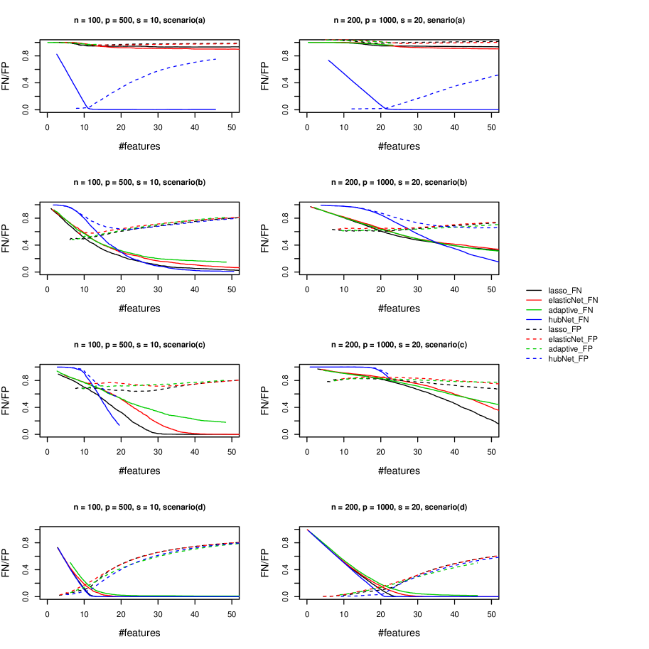
Figure 11: False positive and false negative paths under four generating models.

In Figure 11 of Appendix D, we track FP and FN along the solution paths of the various methods as $\lambda$ varies. The results are in line with the above.

4 Application to real datasets

We compare hubNet with the lasso and elastic net on three real data examples. The following table summarizes the cross-validation errors, test errors, number of selected features, and number of such features in common with those selected by lasso.

Table 5: Comparisons among lasso, elasticNet and hubNet on three real data sets.

cvm(se) Num. features test error common features (lasso) Breast Cancer Data lasso $5.15\%(3.86\%)$ 46 – – $p=806$ elasticNet $5.85\%(3.97\%)$ 303 – 46 $n_{\text{train}}=15359$ hubNet $3.52\%(2.92\%)$ 92 – 26 cvm(se) Num. features test p-value common features (lasso) Kidney Cancer Data lasso 9.89(0.56) 20 0.294 – $p=14814$ elasticNet 9.96(0.56) 11 0.125 9 $n_{\text{train}}=88,n_{\text{test}}=89$ hubNet 9.99(0.42) 1 0.008 0 cvm(se) Num. features test p-value common features (lasso) DLBCL-patient Data lasso 10.9(0.39) 29 0.076 – $p=7399$ elasticNet 10.9(0.39) 37 0.052 28 $n_{\text{train}}=156,n_{\text{test}}=79$ hubNet 11.0(0.24) 2 0.035 0

Example: Lipidomic breast cancer data

This data, from the lab of RT’s collaborator Livia Schiavinato Eberlin at UT Austin, consists of 806 features measured on 15,359 pixels in tissue images from 24 breast cancer patients. The pixels are divided into two classes, normal and cancer, and we fit a regularized logistic regression model using each procedure. Cross-validation classification errors are shown in Figure 4 as $\lambda$ varies. Table 5 reports results for $\lambda$ selected using 5-fold cross-validation.

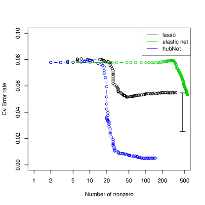
Figure 4: Breast cancer data classification error rates

Example: B cell lymphoma gene expression data

This data from Rosenwald et al. (2002) consists of survival times (observed or right-censored) and 7399 gene expression features for 240 patients with diffuse large B-cell lymphoma (DLBCL). We divided the data with survival time $Y>0$ into 156 training and 79 test samples, and trained a regularized proportional hazards model using each procedure. The p-value of the log-likelihood ratio (LR) statistic of this trained model evaluated on the test set is shown in the left subplot of Figure 5 as $\lambda$ varies. Table 5 reports results for $\lambda$ selected using 20-fold cross-validation.

Example: Kidney cancer gene expression data

This data from Zhao et al. (2005) consists of survival times and 14,814 gene expression features for 177 patients with conventional renal cell carcinoma. We divided the data into 88 training samples and 89 test samples and trained a regularized proportional hazards model using each procedure. For computational reasons, hubNet was fit using the 7999 features with largest absolute row sum in the pairwise correlation matrix; lasso and elastic net were fit using all features. Test set LR p-values are shown in the right subplot of Figure 5 as $\lambda$ varies, and Table 5 reports results for $\lambda$ selected using 8-fold cross validation.

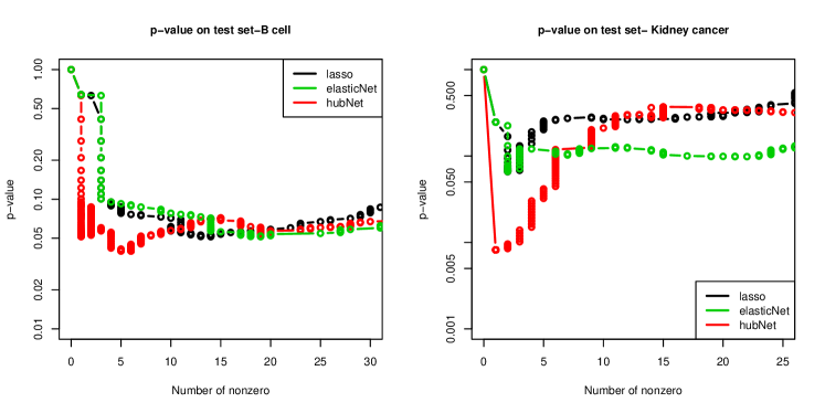
Figure 5: Results for B-cell lymphoma (left) and kidney cancer (right): p-values of LR statistics

5 Theory

In this section, we study recovery of the core set $S$ assuming that our generating model (5, 6) holds. We first establish conditions under which the unsupervised edge-out procedure alone can recover $S$, and then discuss recovery of $S$ by the second adaptive lasso step even if the edge-out procedure does not yield perfect recovery.

We assume the asymptotic regime $n,p\to\infty$ where $s\ll\min(n,p)$, as well as a fully random design where the rows of ${\bf X}$ are independent and distributed as $N(0,{\bf\Sigma})$, normalized so that ${\bf\Sigma}_{jj}=1$ for all $j=1,\ldots,p$. Without loss of generality, we suppose $S$ contains the first $s$ predictors. By (6), if $X:=(X_{S},X_{S^{C}})\sim N(0,{\bf\Sigma})$, then

$$X_{S} \sim N(0,{\bf\Sigma}_{SS}),$$ (11)

$$X_{j}|X_{S} \overset{ind}{\sim}N(X_{S}^{T}\Gamma_{j},\sigma_{j}^{2}),\;\;j\in S^{C}$$ (12)

where $\sigma_{j}^{2}=\operatorname{Var}(\epsilon_{j})\in(0,1)$. Specifically, ${\bf\Gamma}:=(\Gamma_{s+1},\ldots,\Gamma_{p})$ is given by ${\bf\Sigma}_{SS}^{-1}{\bf\Sigma}_{SS^{C}}$. We assume that this model holds in all of the results that follow.

5.1 Recovery of the core set using the edge-out procedure

We analyze recovery of $S$ by the edge-out procedure applied with only the group-lasso penalty term in (8), corresponding to the setting $\gamma=0$. For any matrix ${\bf M}$, denote by ${\bf M}_{i,.}$ and ${\bf M}_{.,j}$ the $i$th row and $j$th column of ${\bf M}$. We use the following operator norms which measure the maximum $\ell_{1}$ and $\ell_{2}$ norm of any row of ${\bf M}$:

$$\|{\bf M}\|_{\infty}:=\sup_{\|x\|_{\infty}=1}\|{\bf M}x\|_{\infty}=\max_{i}\|{\bf M}_{i,.}\|_{1},\hskip 36.135pt\|{\bf M}\|_{\infty,2}:=\sup_{\|x\|_{2}=1}\|{\bf M}x\|_{\infty}=\max_{i}\|{\bf M}_{i,\cdot}\|_{2}.$$

We define also the usual spectral norm, given by the largest singular value of ${\bf M}$,

$$\|{\bf M}\|_{2}:=\sup_{\|x\|_{2}=1}\|{\bf M}x\|_{2}=\sigma_{\max}({\bf M}).$$

We show that in the asymptotic regime $n,p\to\infty$, the edge-out procedure can recover the true core set $S$ for a suitable choice of the tuning parameter $\theta$ when the following conditions hold:

Assumption 5.1

Let $\lambda_{\min}({\bf\Sigma}_{SS})$ be the smallest eigenvalue of ${\bf\Sigma}_{SS}$. For a fixed constant $C_{\min}>0$, $\lambda_{\min}({\bf\Sigma}_{SS})\geq C_{\min}$.

Assumption 5.2

Define ${\bf D}:=\operatorname{diag}(1/\|\Gamma_{s+1}\|_{2},\ldots,1/\|\Gamma_{p}\|_{2})$. For a fixed constant $\delta\in(0,1]$,

$$\|{\bf\Gamma}^{T}{\bf D}{\bf\Gamma}\|_{\infty,2}\leq 1-\delta.$$

Assumption 5.3

(Number of hub nodes). The size $s$ of the core set satisfies

$$s\ll\min(\sqrt{n},n/\log p).$$

Assumption 5.4

(Hub strength). The minimum hub strength $\Gamma_{\min}=\min_{i}\|{\bf\Gamma}_{i,.}\|_{2}$ satisfies

$$\Gamma_{\min}\gg\max(\|{\bf\Gamma}^{T}\|_{\infty},1)\|{\bf\Sigma}_{SS}^{-1}\|_{\infty}\max(1,\sqrt{p/n},\sqrt{p\log p}/n).$$

Under these assumptions, we can ensure perfect recovery of the core set $S$ by the edge-out method:

Theorem 5.5

Let $\hat{{\bf B}}:=\hat{{\bf B}}_{eo}$ be the edge-out estimate in (8) applied with $\gamma=0$, and denote $\hat{S}=\{i:\|\hat{{\bf B}}_{i,.}\|_{2}>0\}$. Suppose Assumptions 5.1, 5.2, 5.3, and 5.4 hold. Defining $\theta_{n}=\theta\sqrt{p-1}/n$, if the tuning parameter $\theta$ is chosen so that

$$\frac{\Gamma_{\min}}{\max(\|{\bf\Gamma}^{T}\|_{\infty},1)\|{\bf\Sigma}_{SS}^{-1}\|_{\infty}}\gg\theta_{n}\gg\max\left(1,\sqrt{\frac{p}{n}},\frac{\sqrt{p\log p}}{n}\right),$$ (13)

then

$$P[\hat{S}=S]\to 1.$$

Assumption 5.1 ensures that the hub features are not too correlated. Assumptions 5.3 and 5.4 restrict the maximal size of the core set and minimal “strength” of the hub features, as measured by the minimum $\ell_{2}$ row norm of ${\bf\Gamma}$. Let us remark that our normalization implies an additional implicit constraint on $s$, namely $p\geq\sum_{j\in S^{C}}\operatorname{Var}(X_{j})=\sum_{j\in S^{C}}\Gamma_{j}^{T}{\bf\Sigma}_{SS}\Gamma_{j}+\sigma_{j}^{2}\geq\|{\bf\Gamma}\|_{F}^{2}C_{\min}\geq sC_{\min}\Gamma_{\min}^{2}$, so by Assumption 5.4

$$s\ll\frac{\min(n,p,n^{2}/\log p)}{\max(\|{\bf\Gamma}^{T}\|_{\infty},1)^{2}\|{\bf\Sigma}_{SS}^{-1}\|_{\infty}^{2}}.$$

In the worst case, we have the upper bounds $\|{\bf\Sigma}_{SS}^{-1}\|_{\infty}\leq\sqrt{s}\|{\bf\Sigma}_{SS}^{-1}\|_{2}\leq\sqrt{s}/C_{\min}$ and $\|{\bf\Gamma}^{T}\|_{\infty}\leq\sqrt{s}\|{\bf\Gamma}^{T}\|_{\infty,2}\leq\sqrt{s/C_{\min}}$, where the latter bound follows from our normalization condition

$$\|{\bf\Gamma}^{T}\|_{\infty,2}^{2}C_{\min}\leq\max_{j\in S^{C}}\Gamma_{j}^{T}{\bf\Sigma}_{SS}\Gamma_{j}\leq\operatorname{Var}(X_{j})\leq 1.$$ (14)

Assuming $\log p\ll\sqrt{n}$, recovery can occur in this worst case when $s\ll\min(n^{1/3},p^{1/3})$. In the best case where an “irrepresentable condition” $\|{\bf\Gamma}^{T}\|_{\infty}\leq 1$ holds (see below) and ${\bf\Sigma}_{SS}=\mathbf{Id}$, then we have $\max(\|{\bf\Gamma}^{T}\|_{\infty},1)\|{\bf\Sigma}_{SS}^{-1}\|_{\infty}=1$, and recovery can occur for $s\ll\min(\sqrt{n},p)$.

Assumption 5.2 is analogous to but much weaker than the “irrepresentable condition” of Zhao and Yu (2006) (see also Wainwright (2009)) that is required for perfect support recovery by the standard lasso procedure. In our random design setting, the irrepresentable condition corresponds to

$$\|{\bf\Gamma}^{T}\|_{\infty}\leq 1-\delta$$ (15)

for some $\delta\in(0,1]$. When (15) holds, Assumption 5.2 is implied by $\|{\bf\Gamma}^{T}{\bf D}{\bf\Gamma}\|_{\infty,2}\leq\|{\bf\Gamma}^{T}\|_{\infty}\|{\bf D}{\bf\Gamma}\|_{\infty,2}=\|{\bf\Gamma}^{T}\|_{\infty}$. The following example illustrates that Assumption 5.2 is weaker than (15):

Example 5.6

Suppose the entries of ${\bf\Gamma}$ are i.i.d. and equal to $(1-2\delta)/\sqrt{s}$ or $-(1-2\delta)/\sqrt{s}$ each with probability 1/2. Then $\|{\bf\Gamma}^{T}{\bf D}{\bf\Gamma}\|_{\infty,2}\leq\|{\bf\Gamma}^{T}\|_{\infty,2}\|{\bf D}\|_{2}\|{\bf\Gamma}\|_{2}=\sqrt{s/(p-s)}\|{\bf\Gamma}\|_{2}$. If $p\to\infty$ with $s\ll p$, the maximal singular value of ${\bf\Gamma}$ satisfies, for any fixed $\varepsilon>0$ with probability approaching 1, $\|{\bf\Gamma}\|_{2}\leq(1+\varepsilon)\sqrt{p}\cdot(1-2\delta)/\sqrt{s}$. (See e.g. Theorem 5.39 of Vershynin (2012).) Hence for large $p$, ${\bf\Gamma}$ satisfies Assumption 5.2 with high probability. However, $\|{\bf\Gamma}^{T}\|_{\infty}=(1-2\delta)\sqrt{s}\gg 1$.

This example shows that Assumption 5.2 can hold even in the worst-case setting where $\|{\bf\Gamma}^{T}\|_{\infty}\asymp\sqrt{s}$, as long as the non-hub features are not influenced by the hub features “in the same way”.

5.2 Recovery of the core set using adaptive lasso

We now consider the linear model (5) where $\epsilon=(\epsilon_{1},\ldots,\epsilon_{p})$ is independent of ${\bf X}$ with $\epsilon_{i}\overset{iid}{\sim}N(0,\sigma^{2})$. We study recovery of $S$ by the adaptive lasso step of the hubNet procedure in two cases: (a) the edge-out estimate yields exact recovery of $S$ , and (b) it yields a superset of $S$.

Let $w_{1},\ldots,w_{p}\in(0,\infty]$ be any feature weights derived from ${\bf X}$. (Setting $w_{i}=\infty$ corresponds to $\|(\hat{{\bf B}}_{eo})_{i,.}\|_{2}=0$, i.e. a hard constraint that requires $\beta_{i}=0$.) Define

$$\rho:=w_{\max}(S)/w_{\min}(S^{C}),\;\;\;\;w_{\min}(S^{c}):=\min_{i\in S^{c}}w_{i},\;\;\;\;w_{\max}(S):=\max_{i\in S}w_{i},$$

with the convention $\infty/\infty=\infty$. We consider the following conditions as $n,p\to\infty$:

Assumption 5.7

There exists $\eta\in(0,1]$ such that with probability approaching 1,

$$\rho\sqrt{\frac{s}{C_{\min}}}\left(1+\sqrt{\frac{12\log p}{n}}\right)\leq 1-\eta.$$

Assumption 5.8

The minimum predictor strength $\beta_{\min}=\min_{i\in S}|\beta^{*}_{i}|$ satisfies

$$\beta_{\min}\gg\sigma\sqrt{\frac{s\log p}{n}\left(1+\frac{\log p}{n}\right)}.$$

Then, under our model (5) and (6), the following result holds for the adaptive lasso:

Theorem 5.9

Let $n,p\to\infty$ such that $s\ll n$ and Assumption 5.1 holds. Furthermore, let $w_{1},\ldots,w_{p}\in(0,\infty]$ be weights (depending on ${\bf X}$) such that Assumption 5.7 holds. Denote by $\hat{\beta}_{0},\hat{\beta}$ the estimator minimizing the adaptive lasso objective (4), and let $\hat{S}=\{i:\hat{\beta}_{i}\neq 0\}$.

(a) Denoting $\lambda_{n}=\lambda/n$, if the tuning parameter $\lambda$ of the adaptive lasso is chosen such that

$$\lambda_{n}\gg\frac{1}{w_{\min}(S^{C})}\sigma\sqrt{\frac{\log p}{n}\left(1+\frac{\log p}{n}\right)}$$

with probability approaching 1, then

$$P[\hat{S}\subseteq S]\to 1.$$

(b) If, in addition, Assumption 5.8 holds and $\lambda_{n}\ll\beta_{\min}/(w_{\max}(S)\sqrt{s})$ with probability approaching 1, then

$$P(\hat{S}=S)\to 1.$$

This result holds for any procedure that selects $w_{1},\ldots,w_{p}$ using ${\bf X}$. Assumption 5.8 is comparable to the beta-min condition in Theorem 3 of Wainwright (2009) for the standard lasso procedure, if $\sqrt{s}$ is replaced by $\|{\bf\Sigma}_{SS}^{-1/2}\|_{\infty}^{2}$. In the context of hubNet, Assumption 5.7 should be interpreted as a weakening of the conditions required for selection consistency of $S$ by the edge-out procedure alone: If the edge-out procedure successfully recovers $S$, then $w_{\min}(S^{c})=\infty$ and $w_{\max}(S)<\infty$, so Assumption 5.7 holds. More generally, Assumption 5.7 holds when there is a separation in size between the rows of $\hat{{\bf B}}_{eo}$ belonging to $S$ and to $S^{C}$, even if the rows belonging to $S^{C}$ are not identically 0.

We prove Theorems 5.5 and 5.9 in Appendix B. The proof of Theorem 5.9 is a simple application of the Sign Recovery Lemma in Zhou et al. (2009) for the adaptive lasso procedure. A more refined statement of Theorem 5.9 in terms of the quantities $\|{\bf\Gamma}^{T}\|_{\infty}$ and $\|{\bf\Sigma}_{SS}^{-1}\|_{\infty}$, similar to that of Theorem 5.5, is possible, although we have stated the above version for simplicity and interpretability.

6 Further topics

6.1 Adaptive, non-linear models

We can extend our basic model (6) to allow the dependence of $Y$ on the core set of predictors to be of a more general form:

$$Y = f({\bf X}_{S})+\epsilon$$ (16)

$$X_{j} = {\bf X}_{S}\Gamma_{j}+\epsilon_{j},j\notin S$$ (17)

Here $f(\cdot)$ is a general, non-linear function. For this model, we can estimate hub weights $s_{j}$ as before and then apply a more flexible prediction procedure such as random forests or gradient boosting using the $s_{j}$ as feature weights. With random forests, the candidate predictors for splitting are chosen at random. Hence it is natural to implement feature weighting by using the weights to determine the probabilities in this sampling. For example, the ranger package in R provides this option.

We tried this idea in the example of Figure 2, with additional interactions $.5x_{1}x_{2}$ and $-2x_{2}x_{3}$ added to the mean of $Y$, so that there were interactions for the random forest to find. We used sampling probabilities proportional to $s_{j}^{2}$. In Figure 6 we show the ratio of the mean squared error of the hubNet/RF over that for the vanilla random forest, as the error standard deviation $\sigma$ is varied. We see that the hub weights can decrease the mean squared error by as much as 15%.

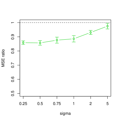
Figure 6: MSE ratio of the hub-weighted random forest to the standard random forest, for varying error standard deviation

6.2 Random forests: a drug discovery application

We consider classification data collected by the NCI, described in Feng et al. (2003) and analyzed further in Chipman et al. (2010). It consists of $p=266$ molecular characteristics of $n=29,374$ compounds, of which $542$ were classified as active ($Y=1$). These predictors represent topological aspects of molecular structure. We randomly created training and test sets of equal size, and for computational reasons we downsampled the class 0 cases to a set of size 2000 out of the 14,687 class 0s in the training set. We applied both random forests and hubNet/RF, using the ranger package in R. The results in Figure 7 show that the hubNet weighting can reduce the number of features by a factor of about 10 (down to 28) with barely any loss in accuracy, and these 28 features would not be detectable from standard RF importance scores (right panel).

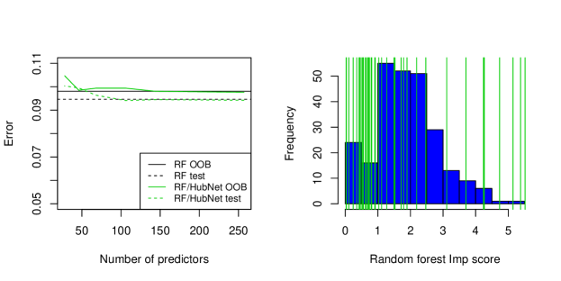
Figure 7: Results for drug discovery dataset. Left panel show out-of-bag error and test error for vanilla random forest (horizontal lines), and the same for hubNet/RF as a function of the number of features having non-zero hub weights (by varying $\theta$ in the edge-out model). We see that the error increases very little, even as the number of number of features is reduced to about one-tenth (28) of the total number. These 28 features are indicated by the green lines in the right panel, superimposed on the RF impurity importance scores for all features.

6.3 Post-selection inference

Since the construction of weights in the hubNet procedure is unsupervised, we can apply recently developed post-selection inference tools for the lasso. In particular, Lee et al. (2016) construct p-values and confidence intervals for the lasso that have exact type I error control and coverage, conditional on the active set of predictors chosen. We can apply these methods to the output of hubNet, since the estimation is just a lasso with weights. Figure 8 shows the 90% post-selection confidence intervals for a realization from the setting of Figure 2, for lasso (left panel) and hubNet (right panel). For the lasso, we see there are no coefficients whose intervals are away from zero, and the intervals are very wide. The hubNet intervals are much shorter, and correctly detect the non-zero coefficients (first three predictors).

Figure 8: 90% post-selection confidence intervals for a realization from the setting of Figure 2, for lasso (left panel) and hubNet (right panel). Note the different vertical scales in the two plots.

7 Recovery of hub nodes and speed comparisons

In this section, we compare the edge-out method with the hglasso method of Tan et al. (2014) in terms of computational speed and recovery of the underlying structure. We generate ${\bf X}$ according to three settings:

1. For a core set $S$ of size $s$, let ${\bf A}\in\{0,1\}^{p\times p}$ have all diagonal entries 1, all entries in row $i$ and column $i$ equal to 1 for all $i\in S$, and remaining entries 0. Define

   $${\bf E}=\begin{cases}0&{\bf A}_{ij}=0\\ \operatorname{Unif}([-0.15,-0.015]\cup[0.015,0.15])&\text{otherwise,}\end{cases}$$

   $\bar{{\bf E}}=\frac{1}{2}({\bf E}+{\bf E}^{T})$, and ${\bf\Sigma}^{-1}=\bar{{\bf E}}+(0.2-\lambda_{\min}(\bar{{\bf E}}))\mathbf{Id}$, and generate the rows of ${\bf X}$ from $N(0,{\bf\Sigma})$.
   

2. For two predictor sets $S_{1}$ and $S_{2}$ of sizes $s/2$, let

   $${\bf A}=\begin{pmatrix}{\bf A}_{1}&0\\ 0&{\bf A}_{2}\end{pmatrix}$$

   with ${\bf A}_{1},{\bf A}_{2}$ generated as above with core sets $S_{1},S_{2}$. Construct ${\bf X}$ from ${\bf A}$ in the same way as above.

3. For a core set $S$ of size $s$, generate ${\bf\Gamma}\in{}^{s\times(p-s)}$ with i.i.d. entries distributed as $N(0,4)$ truncated above and below at $\pm 2$. Then generate each row ${\bf X}_{i,.}$ of ${\bf X}$ such that ${\bf X}_{ij}\sim N(0,1)$ for $j\in S$ and ${\bf X}_{ij}={\bf X}_{i,S}{\bf\Gamma}_{.,j}+\epsilon_{ij}$ for $j\notin S$ and $\epsilon_{ij}\sim N(0,1)$.

In each setting, we re-standardize the predictors to have variance 1.

In Figure 9, we set $(n,p,s)=(100,200,4)$ and compare edge-out and hglasso by the number of correctly identified hub nodes as well as their corresponding absolute row sums in the estimated matrix. (This matrix is $\hat{{\bf B}}_{eo}$ for edge-out and $\hat{{\bf V}}^{T}$ in the hglasso decomposition ${\bf\Sigma}^{-1}={\bf Z}+{\bf V}+{\bf V}^{T}$ where ${\bf Z}$ is sparse and ${\bf V}^{T}$ has few non-zero rows.) Edge-out was applied with only the $\ell_{2}$ penalty (eol2) or with $\gamma=0.5$ (eol12), and hglasso with $\lambda_{1}=1000$ and $\lambda_{2}=0.2$ or 0.5. The left column of the figure tracks the number of correctly identified hubs as the main tuning parameter ($\theta$ for edge-out and $\lambda_{3}$ for hglasso) varies, while the right column tracks the maximum rank of any hub node when all nodes are ranked in decreasing order of their absolute row sums. (A maximum rank of 4 indicates that all four hub nodes have larger absolute row sums than all remaining nodes.) Both variants of edge-out perform well in all three settings; hglasso performs well in settings 1 and 3 for $\lambda_{2}=0.2$ but not for setting 2 under the tested tuning parameters.

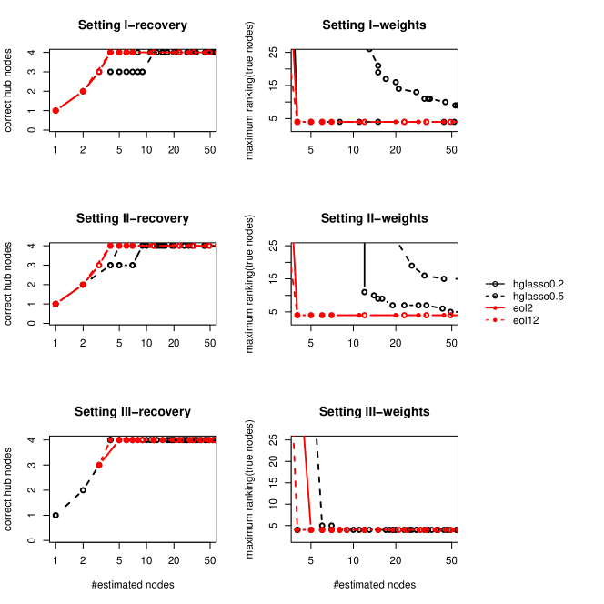
Figure 9: Recovery results and weights ranking

Figure 10 compares the speed of these two methods, with one of $n,p$ fixed while the other grows. We see that the edge-out algorithm is much faster and appears to scale quadratically in $p$ and linearly in $n$.

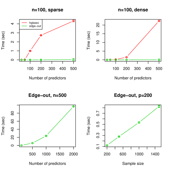
Figure 10: Speed comparisons. In the top row we compare the computation times for the hglasso and edge-out algorithms, as the number of predictors increases, for sparse and dense problems. The bottom row examines just edge-out, with $n$ or $p$ fixed, for larger problems. We were not able to run hglasso in these latter settings.

8 Discussion

We have proposed a new procedure, hubNet, that is applicable to many supervised learning problems. The procedure estimates “hub weights” from the matrix of predictor values and then uses these weights in a supervised learning method such as the lasso or random forest.

HubNet provides a way of utilizing structural information in the predictors, and it can yield more accurate prediction and support recovery in certain situations known to be hard if we neglect such knowledge. Since the estimation of weights is done in an unsupervised manner, standard cross-validation can be applied in the weighted fitting step. We observe in practice that this new procedure can sometimes yield lower prediction error than the unweighted approach, or give similar prediction error using fewer features. Moreover, the estimation of the hub structure can also be useful for interpretation.

Further work is needed in making the edge-out algorithm for hub estimation more efficient, so that it can be applied to very large datasets.

Acknowledgments

Zhou Fan was supported supported by a Hertz Foundation Fellowship and an NDSEG Fellowship (DoD AFOSR 32 CFR 168a). Robert Tibshirani was supported by NIH grant 5R01 EB001988-16 and NSF grant DMS1208164.

Appendix A Optimization for the edge-out model

We consider the objective function (8). The diagonal elements of ${\bf B}$ are fixed at zero. Let ${\bf X}_{.,i}$ and ${\bf X}_{.,-i}$ denote the $i$th column of ${\bf X}$ and ${\bf X}$ with $i$th column removed, and let ${\bf B}_{-i,-i}$ denote ${\bf B}$ with $i$th row and column both removed. Let $S(x,t)={\rm sign}(x)(|x|-t)_{+}$ be the soft-thresholding operator.

We use the following blockwise coordinate descent algorithm similar to that of Peng et al. (2010):

1. Initialize ${\bf B}=0$.

2. Iterate over $i\in\{1,2,\ldots,p\}$ until convergence:

   1. Compute the $1\times(p-1)$ vector $\mathbf{r}_{i,-i}={\bf X}_{.,i}^{T}({\bf X}_{.,-i}-{\bf X}_{.,-i}{\bf B}_{-i,-i})$.

   2. Compute the elementwise soft-thresholded vector $\beta_{i,-i}=S(\mathbf{r}_{i,-i},\theta\gamma)$.

   3. Update the $i$th row of ${\bf B}$:

      $${\bf B}_{i,-i}=\begin{cases}0&\|\beta_{i,-i}\|_{2}\|{\bf X}_{.,i}\|^{2}_{2}\leq\theta(1-\gamma)\sqrt{p-1}\\ (1-\frac{\theta(1-\gamma)\sqrt{p-1}}{\|\beta_{i.-i}\|_{2}\|{\bf X}_{.,i}\|^{2}_{2}})\beta_{i,-i}&\|\beta_{i,-i}\|_{2}\|{\bf X}_{.,i}\|^{2}_{2}>\theta(1-\gamma)\sqrt{p-1}\end{cases}$$

It can be shown that, fixing all entries of ${\bf B}$ not in row $i$, the above update expression exactly minimizes the objective over ${\bf B}_{i,-i}$. Then this procedure is a blockwise coordinate descent algorithm, applied to an objective whose non-differentiable component is separable across blocks, and hence converges to the solution.

Appendix B Proof of Theorems 5.5 and 5.9

Denote by ${\bf X}_{S}$ and ${\bf X}_{S^{C}}$ the submatrices of ${\bf X}$ consisting of predictors in $S$ and $S^{C}$, and define

$$\hat{{\bf\Sigma}}_{SS}:=\frac{1}{n}{\bf X}_{S}^{T}{\bf X}_{S},\;\;\;\;\hat{{\bf\Sigma}}_{S^{C}S}:=\frac{1}{n}{\bf X}_{S^{C}}^{T}{\bf X}_{S},\;\;\;\;{\bf W}:={\bf X}_{S^{C}}-{\bf X}_{S}{\bf\Gamma}.$$

Note that by (6), ${\bf W}$ is independent of ${\bf X}_{S}$ with independent Gaussian entries of variance at most 1. The following lemma collects probabilistic statements involving ${\bf X}_{S}$ and ${\bf W}$; its proof is deferred to Appendix C.

Lemma B.1

Suppose $n,p\to\infty$, $1\leq s\leq p$, and $s\ll n$. If $\lambda_{\min}({\bf\Sigma}_{SS})\geq C_{\min}$ for a constant $C_{\min}>0$, then each of the following statements holds with probability approaching 1:

$$\max_{j=1}^{p}\|{\bf X}_{.,j}\|^{2} \leq 2n+6\log p$$ (18)

$$\max_{j=1}^{s}\|{\bf X}_{.,j}\|^{2} \leq 2n$$ (19)

$$\|\hat{{\bf\Sigma}}^{-1}_{SS}\|_{2} \leq 2C_{\min}^{-1}$$ (20)

$$\|\hat{{\bf\Sigma}}^{-1}_{SS}\|_{\infty} \leq\|{\bf\Sigma}_{SS}^{-1}\|_{\infty}+3(s+\sqrt{s}\log n)/(C_{\min}\sqrt{n})$$ (21)

$$\|\hat{{\bf\Sigma}}_{SS}^{-1}{\bf X}_{S}^{T}{\bf W}\|_{\infty,2} \leq\sqrt{4np/C_{\min}}$$ (22)

$$\|{\bf W}^{T}{\bf X}_{S}\hat{{\bf\Sigma}}_{SS}^{-1}\|_{\infty,2} \leq\sqrt{4n(s+3\log p)/C_{\min}}$$ (23)

$$\|{\bf W}^{T}(\mathbf{Id}_{s\times s}-\tfrac{1}{n}{\bf X}_{S}\hat{{\bf\Sigma}}_{SS}^{-1}{\bf X}_{S}^{T}){\bf W}\|_{\infty,2} \leq 2n+\sqrt{3np}+\sqrt{6p\log p}.$$ (24)

Proof of Theorem 5.5

Our proof draws upon a similar analysis of support recovery in the multivariate regression setting by Obozinski et al. (2011). Let us introduce $\theta_{n}=\theta\sqrt{p-1}/n$ and write the edge-out estimate (in the case $\gamma=0$) as

$$\hat{{\bf B}}_{eo}=\operatorname*{arg\,min}_{{\bf B}\in{}^{p\times p}:\,{\bf B}_{ii}=0\,\forall i}\frac{1}{2n}\|{\bf X}-{\bf X}{\bf B}\|^{2}_{F}+\theta_{n}\sum_{i=1}^{p}\|{\bf B}_{i,.}\|_{2}.$$ (25)

Consider the restricted problem over ${\bf B}\in{}^{s\times p}$ where each predictor is regressed only on ${\bf X}_{S}$:

$$\hat{{\bf B}}_{\text{restricted}} =\operatorname*{arg\,min}_{{\bf B}\in{}^{s\times p}:\,{\bf B}_{ii}=0\,\forall i}\frac{1}{2n}\|{\bf X}-{\bf X}_{S}{\bf B}\|^{2}_{F}+\theta_{n}\sum_{i\in S}\|{\bf B}_{i,.}\|_{2}.$$ (26)

The subgradient conditions for optimality of $\hat{{\bf B}}_{eo}$ and $\hat{{\bf B}}_{\text{restricted}}$ imply the following sufficient condition for recovery of $S$, whose proof we defer to Appendix C:

Lemma B.2

If ${\bf X}_{S}^{T}{\bf X}_{S}$ is invertible, then the solution $\hat{{\bf B}}:=\hat{{\bf B}}_{\text{restricted}}$ to (26) is unique. If furthermore this solution satisfies

$$\max_{j\in S^{c}}\frac{1}{n}\|{\bf X}_{\cdot,j}^{T}({\bf X}-{\bf X}_{S}\hat{{\bf B}})\|_{2} <\theta_{n},$$ (27)

$$\min_{i\in S}\|\hat{{\bf B}}_{i,.}\|_{2} >0,$$ (28)

then the solution $\hat{{\bf B}}_{eo}$ to (25) is unique, with the first $s$ rows non-zero and equal to $\hat{{\bf B}}$ and remaining rows equal to 0.

Through the remainder of this appendix, let $\hat{{\bf B}}:=\hat{{\bf B}}_{\text{restricted}}\in{}^{s\times p}$ be the solution to the restricted problem (26). As $s\ll n$ and ${\bf\Sigma}_{SS}$ is non-singular, ${\bf X}_{S}^{T}{\bf X}_{S}$ is invertible with probability 1. Hence, to prove Theorem 5.5, it suffices to show that (27) and (28) hold with high probability. Define

$${\bf U} :=\begin{pmatrix}\mathbf{Id}_{s\times s}&\frac{1}{n}\hat{{\bf\Sigma}}_{SS}^{-1}{\bf X}_{S}^{T}{\bf W}\end{pmatrix}\in{}^{s\times p},$$

$${\bf B}^{*} :=\begin{pmatrix}\mathbf{0}_{s\times s}&{\bf\Gamma}\end{pmatrix}\in{}^{s\times p},$$

$$\hat{{\bf D}} :=\operatorname{diag}\left(\|\hat{{\bf B}}_{1,.}\|^{-1}_{2},...,\|\hat{{\bf B}}_{s,.}\|^{-1}_{2}\right)\in{}^{s\times s},$$

$${\bf\Delta} \in{}^{s\times p},\;\;{\bf\Delta}_{ij}:=\begin{cases}{\bf X}^{T}_{.,j}({\bf X}_{.,j}-{\bf X}_{S}\hat{{\bf B}}_{.,j})&i=j\\ 0&\text{otherwise},\end{cases}$$

$$\mathcal{Z} :=\left\{{\bf Z}\in[-1,1]^{s\times p}:\begin{array}[]{ll}{\bf Z}_{i,.}=\hat{{\bf D}}_{i,i}\hat{{\bf B}}_{i,.}&\mbox{ if }\|\hat{{\bf B}}_{i,.}\|_{2}>0\\ {\bf Z}_{i,i}=0\text{ and }\|{\bf Z}_{i,.}\|_{2}\leq 1&\mbox{ if }\|\hat{{\bf B}}_{i,.}\|_{2}=0\end{array}\right\}$$

The subgradient condition for optimality of $\hat{{\bf B}}$ for (26) implies the following, whose proof we also defer to Appendix C.

Lemma B.3

There exists ${\bf Z}\in\mathcal{Z}$ such that

$$\hat{{\bf B}}-{\bf B}^{*}={\bf U}-\theta_{n}\hat{{\bf\Sigma}}_{SS}^{-1}{\bf Z}-\tfrac{1}{n}\hat{{\bf\Sigma}}_{SS}^{-1}{\bf\Delta}.$$

Using these lemmas, we now verify conditions (27) and (28):

Lemma B.4

Suppose Assumptions 5.1, 5.3, and 5.4 hold, and $\theta_{n}$ satisfies (13). Then with probability approaching 1, (28) holds and

$$\|\hat{{\bf B}}-{\bf B}^{*}\|_{\infty,2}\leq 2\theta_{n}\|{\bf\Sigma}_{SS}^{-1}\|_{\infty}.$$

Proof:

By Lemma B.3, for some ${\bf Z}\in\mathcal{Z}$,

$$\|\hat{{\bf B}}-{\bf B}^{*}\|_{\infty,2}\leq\|{\bf U}\|_{\infty,2}+\theta_{n}\|\hat{{\bf\Sigma}}_{SS}^{-1}{\bf Z}\|_{\infty,2}+\tfrac{1}{n}\|\hat{{\bf\Sigma}}_{SS}^{-1}{\bf\Delta}\|_{\infty,2}.$$

For the first term, (22) and the definition of ${\bf U}$ imply, with probability approaching 1,

$$\|{\bf U}\|_{\infty,2}\leq 1+\sqrt{4p/(C_{\min}n)}.$$

For the second term, (21) and the observation $\|{\bf Z}\|_{\infty,2}\leq 1$ imply, with probability approaching 1,

$$\|\hat{{\bf\Sigma}}_{SS}^{-1}{\bf Z}\|_{\infty,2}\leq\|\hat{{\bf\Sigma}}_{SS}^{-1}\|_{\infty}\|{\bf Z}\|_{\infty,2}\leq\|\hat{{\bf\Sigma}}_{SS}^{-1}\|_{\infty}\leq\|{\bf\Sigma}_{SS}^{-1}\|+3(s+\sqrt{s}\log n)/(C_{\min}\sqrt{n}).$$

For the third term, note that for all $j=1,\ldots,p$,

$$|{\bf\Delta}_{jj}|\leq\|{\bf X}_{.,j}\|^{2},$$ (29)

for otherwise

$$\|{\bf X}_{.,j}-{\bf X}_{S}\hat{{\bf B}}_{.,j}\|_{2}^{2}-\|{\bf X}_{.,j}\|^{2}=(2{\bf X}_{.,j}-{\bf X}_{S}\hat{{\bf B}}_{.,j})^{T}(-{\bf X}_{S}\hat{{\bf B}}_{.,j})>0,$$

implying that the objective (26) would decrease upon setting $\hat{{\bf B}}_{.,j}=0$ and contradicting optimality of $\hat{{\bf B}}$. Then, as ${\bf\Delta}$ is diagonal, (19) and (20) imply, with probability approaching 1,

$$\|\hat{{\bf\Sigma}}_{SS}^{-1}{\bf\Delta}\|_{\infty,2}\leq\|\hat{{\bf\Sigma}}_{SS}^{-1}\|_{\infty,2}\max_{j=1}^{s}|{\bf\Delta}_{jj}|\leq\|\hat{{\bf\Sigma}}_{SS}^{-1}\|_{2}\max_{j=1}^{s}\|{\bf X}_{.,j}\|_{2}^{2}\leq 4n/C_{\min}.$$

Noting that $\|{\bf\Sigma}_{SS}^{-1}\|_{\infty}\geq\|{\bf\Sigma}_{SS}^{-1}\|_{2}=1/\lambda_{\min}({\bf\Sigma}_{SS})\geq 1$ by our normalization ${\bf\Sigma}_{jj}=1$ for all $j$, we have under the given assumptions

$$\max(1,\sqrt{p/n},\theta_{n}s/\sqrt{n},\theta_{n}\sqrt{s/n}\log n,\ll\theta_{n}\|{\bf\Sigma}_{SS}^{-1}\|_{\infty}\ll\Gamma_{\min}.$$

Then with probability approaching 1, $\|\hat{{\bf B}}-{\bf B}^{*}\|_{\infty,2}\leq 2\theta_{n}\|{\bf\Sigma}_{SS}^{-1}\|_{\infty}$ and

$$\min_{i}\|\hat{{\bf B}}_{i,.}\|_{2}\geq\min_{i}\|{\bf B}^{*}_{i,.}\|_{2}-2\theta_{n}\|{\bf\Sigma}_{SS}^{-1}\|_{\infty}=\Gamma_{\min}-2\theta_{n}\|{\bf\Sigma}_{SS}^{-1}\|_{\infty}>0.$$

$\blacksquare$

Lemma B.5

Suppose Assumptions 5.1, 5.2, 5.3, and 5.4 hold, and $\theta_{n}$ satisfies (13). Then (27) holds with probability approaching 1.

Proof: By Lemma B.4, it suffices to consider the event where $\|\hat{{\bf B}}_{i,.}\|_{2}>0$ for all $i\in S$, and hence ${\bf Z}=\hat{{\bf D}}\hat{{\bf B}}$ in Lemma B.3. On this event, writing ${\bf X}=({\bf X}_{S},{\bf X}_{S}{\bf\Gamma}+{\bf W})=({\bf X}_{S},{\bf W})+{\bf X}_{S}{\bf B}^{*}$ and applying Lemma B.3,

$$\frac{1}{n}\|{\bf X}^{T}_{S^{C}} ({\bf X}-{\bf X}_{S}\hat{{\bf B}})\|_{\infty,2}=\frac{1}{n}\|{\bf X}^{T}_{S^{C}}({\bf X}_{S},{\bf W})+{\bf X}_{S^{C}}^{T}{\bf X}_{S}({\bf B}^{*}-\hat{{\bf B}})\|_{\infty,2}$$

$$\leq\frac{1}{n}\|{\bf X}^{T}_{S^{C}}({\bf X}_{S},{\bf W})-{\bf X}_{S^{C}}^{T}{\bf X}_{S}{\bf U}\|_{\infty,2}+\theta_{n}\|\hat{{\bf\Sigma}}_{S^{C}S}\hat{{\bf\Sigma}}_{SS}^{-1}\hat{{\bf D}}\hat{{\bf B}}\|_{\infty,2}+\frac{1}{n}\|\hat{{\bf\Sigma}}_{S^{C}S}\hat{{\bf\Sigma}}_{SS}^{-1}{\bf\Delta}\|_{\infty,2}.$$ (30)

For the first term of (30), recalling the definition of ${\bf U}$, noting that ${\bf X}_{S}^{T}(\mathbf{Id}-\frac{1}{n}{\bf X}_{S}\hat{{\bf\Sigma}}_{SS}^{-1}{\bf X}_{S}^{T})=0$, and applying (24), with probability approaching 1,

$$\|{\bf X}^{T}_{S^{C}}({\bf X}_{S},{\bf W}) -{\bf X}_{S^{C}}^{T}{\bf X}_{S}{\bf U}\|_{\infty,2}=\|{\bf X}_{S^{C}}^{T}(\mathbf{Id}-\tfrac{1}{n}{\bf X}_{S}\hat{{\bf\Sigma}}_{SS}^{-1}{\bf X}_{S}^{T}){\bf W}\|_{\infty,2}$$

$$=\|{\bf W}^{T}(\mathbf{Id}-\tfrac{1}{n}{\bf X}_{S}\hat{{\bf\Sigma}}_{SS}^{-1}{\bf X}_{S}^{T}){\bf W}\|_{\infty,2}\leq 2n+\sqrt{3np}+\sqrt{6p\log p}\ll n\theta_{n}.$$

For the third term of (30), applying (29), (14), (19), and (23), with probability approaching 1,

$$\|\hat{{\bf\Sigma}}_{S^{C}S}\hat{{\bf\Sigma}}_{SS}^{-1}{\bf\Delta}\|_{\infty,2} \leq\|\hat{{\bf\Sigma}}_{S^{C}S}\hat{{\bf\Sigma}}_{SS}^{-1}\|_{\infty,2}\max_{j=1}^{s}|{\bf\Delta}_{jj}|=\frac{1}{n}\|({\bf X}_{S}{\bf\Gamma}+{\bf W})^{T}{\bf X}_{S}\hat{{\bf\Sigma}}_{SS}^{-1}\|_{\infty,2}\max_{j=1}^{s}|{\bf\Delta}_{jj}|$$

$$\leq\left(\|{\bf\Gamma}^{T}\|_{\infty,2}+\frac{1}{n}\|{\bf W}^{T}{\bf X}_{S}\hat{{\bf\Sigma}}_{SS}^{-1}\|_{\infty,2}\right)\max_{j=1}^{s}\|{\bf X}_{.,j}\|_{2}^{2}\leq\frac{2n}{\sqrt{C_{\min}}}+\sqrt{\frac{16n(s+3\log p)}{C_{\min}}}\ll n\theta_{n}.$$

It remains to bound the second term of (30). Let ${\bf D}$ be as in Assumption 5.2 and write

$$\hat{{\bf\Sigma}}_{S^{C}S}\hat{{\bf\Sigma}}_{SS}^{-1}\hat{{\bf D}}\hat{{\bf B}} ={\bf\Gamma}^{T}{\bf D}{\bf B}^{*}+{\bf\Gamma}^{T}{\bf D}(\hat{{\bf B}}-{\bf B}^{*})+{\bf\Gamma}^{T}(\hat{{\bf D}}-{\bf D})\hat{{\bf B}}+(\hat{{\bf\Sigma}}_{S^{C}S}\hat{{\bf\Sigma}}_{SS}^{-1}-{\bf\Gamma}^{T})\hat{{\bf D}}\hat{{\bf B}}$$

$$=:\mathbf{I}+\mathbf{II}+\mathbf{III}+\mathbf{IV}.$$

By Assumption 5.2 and the definition of ${\bf B}^{*}$,

$$\|\mathbf{I}\|_{\infty,2}=\|{\bf\Gamma}^{T}{\bf D}{\bf\Gamma}\|_{\infty,2}\leq 1-\delta.$$

By Lemma B.4, with probability approaching 1,

$$\|\mathbf{II}\|_{\infty,2}\leq\|{\bf\Gamma}^{T}\|_{\infty}\|{\bf D}(\hat{{\bf B}}-{\bf B}^{*})\|_{\infty,2}\leq\|{\bf\Gamma}^{T}\|_{\infty}\Gamma_{\min}^{-1}\|\hat{{\bf B}}-{\bf B}^{*}\|_{\infty,2}\leq 2\|{\bf\Gamma}^{T}\|_{\infty}\Gamma_{\min}^{-1}\theta_{n}\|{\bf\Sigma}_{SS}^{-1}\|_{\infty}\ll 1.$$

$\mathbf{III}$ satisfies the same bound, as

$$\|\mathbf{III}\|_{\infty,2}\leq\|{\bf\Gamma}^{T}\|_{\infty}\|(\hat{{\bf D}}-{\bf D})\hat{{\bf B}}\|_{\infty,2}=\|{\bf\Gamma}^{T}\|_{\infty}\max_{i\in S}\frac{|\|{\bf B}^{*}_{i,.}\|_{2}-\|\hat{{\bf B}}_{i,.}\|_{2}|}{\|{\bf B}^{*}_{i,.}\|_{2}}\leq\|{\bf\Gamma}^{T}\|_{\infty}\|{\bf D}(\hat{{\bf B}}-{\bf B}^{*})\|_{\infty,2}.$$

Finally, using ${\bf X}_{S^{C}}={\bf X}_{S}{\bf\Gamma}+{\bf W}$ and applying (23), with probability approaching 1,

$$\|\mathbf{IV}\|_{\infty,2} =\|(\tfrac{1}{n}{\bf X}_{S^{C}}^{T}{\bf X}_{S}\hat{{\bf\Sigma}}_{SS}^{-1}-{\bf\Gamma}^{T})\hat{{\bf D}}{\hat{{\bf B}}}\|_{\infty,2}=\frac{1}{n}\|{\bf W}^{T}{\bf X}_{S}\hat{{\bf\Sigma}}_{SS}^{-1}\hat{{\bf D}}\hat{{\bf B}}\|_{\infty,2}$$

$$\leq\frac{1}{n}\|{\bf W}^{T}{\bf X}_{S}\hat{{\bf\Sigma}}_{SS}^{-1}\|_{\infty}\|\hat{{\bf D}}\hat{{\bf B}}\|_{\infty,2}\leq\frac{\sqrt{s}}{n}\|{\bf W}^{T}{\bf X}_{S}\hat{{\bf\Sigma}}_{SS}^{-1}\|_{\infty,2}\leq\sqrt{\frac{4s(s+3\log p)}{C_{\min}n}}\ll 1.$$

Combining the above yields $\|\hat{{\bf\Sigma}}_{S^{C}S}\hat{{\bf\Sigma}}_{SS}^{-1}\hat{{\bf D}}\hat{{\bf B}}\|_{\infty,2}\leq 1-\delta/2$ with probability approaching 1, which together with (30) implies (27).

$\blacksquare$

Theorem 5.5 follows from Lemmas B.2, B.4, and B.5.

Proof of Theorem 5.9

We verify the conditions of Lemma 8.2 of Zhou et al. (2009) under the given assumptions and in our asymptotic setting with random design. By (18) and (20), with probability approaching 1,

$$\max_{j\in S^{C}}\frac{\|{\bf X}_{.,j}\|_{2}}{\sqrt{n}}\leq\sqrt{2+\frac{6\log p}{n}},\;\;\;\;\lambda_{\min}(\hat{{\bf\Sigma}}_{SS})\geq\frac{C_{\min}}{2}.$$ (31)

It remains to verify the weighted incoherency condition (8.4a) of Zhou et al. (2009). Define ${\bf D}_{w,S}=\operatorname{diag}(w_{1},\ldots,w_{s})\in{}^{s\times s}$ and ${\bf D}_{w,S^{C}}^{-1}=\operatorname{diag}(w_{s+1}^{-1},\ldots,w_{p}^{-1})\in{}^{(s-p)\times(s-p)}$ where $w_{k}^{-1}=0$ if $w_{k}=\infty$. Then

$$\|{\bf D}_{w,S^{C}}^{-1}{\bf X}_{S^{C}}^{T}{\bf X}_{S}({\bf X}_{S}^{T}{\bf X}_{S})^{-1}{\bf D}_{w,S}\|_{\infty}\leq\frac{w_{\max}(S)}{nw_{\min}(S^{C})}\|{\bf X}_{S^{C}}^{T}{\bf X}_{S}\hat{{\bf\Sigma}}_{SS}^{-1}\|_{\infty}\leq\frac{\rho}{n}\|{\bf X}_{S^{C}}^{T}{\bf X}_{S}\hat{{\bf\Sigma}}_{SS}^{-1}\|_{\infty}.$$

Writing ${\bf X}_{S^{C}}={\bf X}_{S}{\bf\Gamma}+{\bf W}$ and applying (14) and (23), with probability approaching 1,

$$\frac{1}{n}\|{\bf X}_{S^{C}}^{T}{\bf X}_{S}\hat{{\bf\Sigma}}_{SS}^{-1}\|_{\infty} \leq\frac{\sqrt{s}}{n}\|{\bf X}_{S^{C}}^{T}{\bf X}_{S}\hat{{\bf\Sigma}}_{SS}^{-1}\|_{\infty,2}\leq\sqrt{s}\|{\bf\Gamma}^{T}\|_{\infty,2}+\frac{\sqrt{s}}{n}\|{\bf W}^{T}{\bf X}_{S}{\bf\Sigma}_{SS}^{-1}\|_{\infty,2}$$

$$\leq\sqrt{\frac{s}{C_{\min}}}+\sqrt{\frac{4s(s+3\log p)}{nC_{\min}}}\leq\sqrt{\frac{s}{C_{\min}}}\left(1+\sqrt{\frac{12\log p}{n}}+o(1)\right).$$

Hence under Assumption 5.7, with probability approaching 1,

$$\|{\bf D}_{w,S^{C}}^{-1}{\bf X}_{S^{C}}^{T}{\bf X}_{S}({\bf X}_{S}^{T}{\bf X}_{S})^{-1}{\bf D}_{w,S}\|_{\infty}\leq 1-\eta-o(1)\leq 1-\eta/2.$$ (32)

Conditional on ${\bf X}$, on the event where (31) and (32) hold, our conclusion follows from Lemma 8.2 of Zhou et al. (2009). Then the conclusion also follows unconditionally.

Appendix C Proofs of supporting lemmas

In this appendix, we prove Lemmas B.1, B.2, and B.3.

Proof of Lemma B.1

Our normalization ${\bf\Sigma}_{jj}=1$ implies $\|{\bf X}_{.,j}\|_{2}^{2}\sim\chi^{2}_{n}$ for each $j=1,\ldots,p$. We use the chi-squared tail bound

$$P[\chi_{n}^{2}>n+2\sqrt{nt}+2t]\leq\exp(-t)$$ (33)

for all $t>0$, from Lemma 1 of Laurent and Massart (2000). Then

$$P[\|{\bf X}_{.,j}\|_{2}^{2}>2n+6\log p]\leq P[\|{\bf X}_{.,j}\|_{2}^{2}>n+2\sqrt{2n\log p}+4\log p]\leq\exp(-2\log p),$$

and a union bound over $j=1,\ldots,p$ yields (18). Also, $P[\|{\bf X}_{.,j}\|_{2}^{2}>2n]\leq\exp(-n/8)$, and as $s\ll n$, a union bound over $j=1,\ldots,s$ yields (19). For (20) and (21),

$$\|\hat{{\bf\Sigma}}_{SS}^{-1}-{\bf\Sigma}_{SS}^{-1}\|_{2}\leq\|{\bf\Sigma}_{SS}^{-1/2}\|_{2}\|{\bf\Sigma}_{SS}^{1/2}\hat{{\bf\Sigma}}_{SS}^{-1}{\bf\Sigma}_{SS}^{1/2}-\mathbf{Id}\|_{2}\|{\bf\Sigma}_{SS}^{-1/2}\|_{2}\leq C_{\min}^{-1}\|\tilde{{\bf\Sigma}}_{SS}^{-1}-\mathbf{Id}\|_{2}$$

where $\tilde{{\bf\Sigma}}_{SS}\overset{L}{=}n^{-1}{\bf Z}^{T}{\bf Z}$ for ${\bf Z}\in{}^{n\times s}$ having i.i.d. standard Gaussian entries. Corollary 5.35 of Vershynin (2012) implies

$$\left(1-\frac{\sqrt{s}+\log n}{\sqrt{n}}\right)^{2}\leq\lambda_{\min}(\tilde{{\bf\Sigma}}_{SS})\leq\lambda_{\max}(\tilde{{\bf\Sigma}}_{SS})\leq\left(1+\frac{\sqrt{s}+\log n}{\sqrt{n}}\right)^{2}$$

with probability approaching 1. As $s\ll n$, this implies for any $\delta>0$, with probability approaching 1

$$\|\tilde{{\bf\Sigma}}_{SS}^{-1}-\mathbf{Id}\|_{2}\leq(2+\delta)\left(\frac{\sqrt{s}+\log n}{\sqrt{n}}\right).$$

Then (20) follows from $\|\hat{{\bf\Sigma}}_{SS}^{-1}\|_{2}\leq\|\hat{{\bf\Sigma}}_{SS}^{-1}-{\bf\Sigma}_{SS}^{-1}\|_{2}+\|{\bf\Sigma}_{SS}^{-1}\|_{2}\leq 2C_{\min}^{-1}$, and (21) from

$$\|\hat{{\bf\Sigma}}_{SS}^{-1}\|_{\infty}\leq\|\hat{{\bf\Sigma}}_{SS}^{-1}-{\bf\Sigma}_{SS}^{-1}\|_{\infty}+\|{\bf\Sigma}_{SS}^{-1}\|_{\infty}\leq\sqrt{s}\|\hat{{\bf\Sigma}}_{SS}^{-1}-{\bf\Sigma}_{SS}^{-1}\|_{2}+\|{\bf\Sigma}_{SS}^{-1}\|_{\infty}\leq\frac{3(s+\sqrt{s}\log n)}{C_{\min}\sqrt{n}}+\|{\bf\Sigma}_{SS}^{-1}\|_{\infty}.$$

For the remaining three statements, denote ${\bf S}=\operatorname{diag}(\sigma_{j+1},\ldots,\sigma_{p})\in{}^{(p-s)\times(p-s)}$, so ${\bf W}={\bf Z}{\bf S}$ where ${\bf Z}\in{}^{n\times(p-s)}$ is independent of ${\bf X}_{S}$ with i.i.d. standard Gaussian entries. Denote ${\bf P}=\frac{1}{\sqrt{n}}\hat{{\bf\Sigma}}_{SS}^{-1/2}{\bf X}_{S}^{T}$, so that ${\bf P}^{T}{\bf P}$ is the projection in ⁿ onto the column span of ${\bf X}_{S}$. With probability 1, this column span is of rank $s$, so ${\bf P}$ is an orthogonal projection from ⁿ to ^s. Applying $\sigma_{j}\leq 1$ for each $j$,

$$\|\hat{{\bf\Sigma}}_{SS}^{-1}{\bf X}_{S}^{T}{\bf W}\|_{\infty,2}=\sqrt{n}\|\hat{{\bf\Sigma}}_{SS}^{-1/2}{\bf P}{\bf Z}{\bf S}\|_{\infty,2}\leq\sqrt{n}\|\hat{{\bf\Sigma}}_{SS}^{-1/2}{\bf P}{\bf Z}\|_{\infty,2}.$$

Conditional on ${\bf X}_{S}$, the columns of $\hat{{\bf\Sigma}}_{SS}^{-1/2}{\bf P}{\bf Z}$ are independent and distributed as $N(0,\hat{{\bf\Sigma}}_{SS}^{-1})$, so each $i$th row of $\hat{{\bf\Sigma}}_{SS}^{-1/2}{\bf P}{\bf Z}$ consists of independent Gaussian entries with variance $(\hat{{\bf\Sigma}}_{SS}^{-1})_{ii}\leq\|\hat{{\bf\Sigma}}_{SS}^{-1}\|_{2}$. Then by (33),

$$P[\|(\hat{{\bf\Sigma}}_{SS}^{-1/2}{\bf P}{\bf Z})_{i,.}\|_{2}^{2}>2p\|\hat{{\bf\Sigma}}_{SS}^{-1}\|_{2}\mid{\bf X}_{S}]\leq\exp(-p/8),$$

and (22) follows by taking a union bound over $i=1,\ldots,s$, recalling $s\leq p$, and applying (20). Similarly, $\|{\bf W}^{T}{\bf X}_{S}{\bf\Sigma}_{SS}^{-1}\|_{\infty,2}\leq\sqrt{n}\|{\bf Z}^{T}{\bf P}^{T}{\bf\Sigma}_{SS}^{-1/2}\|_{\infty,2}$, and conditional on ${\bf X}_{S}$ each row of ${\bf Z}^{T}{\bf P}^{T}\hat{{\bf\Sigma}}_{SS}^{-1}$ is distributed as $N(0,\hat{{\bf\Sigma}}_{SS}^{-1})$. Then (33) implies

$$P[\|({\bf Z}^{T}{\bf P}^{T}\hat{{\bf\Sigma}}_{SS}^{-1/2})_{j,.}\|_{2}^{2}>(2s+6\log p)\|\hat{{\bf\Sigma}}_{SS}^{-1}\|_{2}\mid{\bf X}_{S}]\leq\exp(-2\log p),$$

and (20) and a union bound over $j=s+1,\ldots,p$ yields (23). Finally,

$$\|{\bf W}^{T}(\mathbf{Id}-\tfrac{1}{n}{\bf X}_{S}{\bf\Sigma}_{SS}^{-1}{\bf X}_{S}^{T}){\bf W}\|_{\infty,2}\leq\|{\bf Z}^{T}(\mathbf{Id}-{\bf P}^{T}{\bf P}){\bf Z}\|_{\infty,2},$$

and conditional on ${\bf X}_{S}$, ${\bf Z}^{T}(\mathbf{Id}-{\bf P}^{T}{\bf P}){\bf Z}$ is equal in law to $\tilde{{\bf Z}}^{T}\tilde{{\bf Z}}$ where $\tilde{{\bf Z}}\in{}^{(n-s)\times(p-s)}$ has i.i.d. standard Gaussian entries. Writing $\|\tilde{{\bf Z}}^{T}\tilde{{\bf Z}}\|_{\infty,2}\leq\|\tilde{{\bf Z}}^{T}\|_{\infty,2}\|\tilde{{\bf Z}}\|_{2}$, Corollary 5.35 of Vershynin (2012) implies $\|\tilde{{\bf Z}}\|_{2}\leq\sqrt{2n}+\sqrt{p}$ with probability approaching 1, while (33) implies $\|\tilde{{\bf Z}}\|_{\infty,2}^{2}\leq 2n+6\log p$ with probability approaching 1. Then (24) follows from combining these bounds and observing $n\log p\ll np$.

Proof of Lemma B.2

Denote by $J_{eo}({\bf B})$ the objective function in (25) and by $J_{\text{restricted}}({\bf B})$ the objective function in (26). (The former is a function of ${\bf B}\in{}^{p\times p}:{\bf B}_{ii}=0$ and the latter of ${\bf B}\in{}^{s\times p}:{\bf B}_{ii}=0$.) If ${\bf X}_{S}^{T}{\bf X}_{S}$ is invertible, then $J_{\text{restricted}}$ is strictly convex and $|J_{\text{restricted}}({\bf B})|\to\infty$ as $\|{\bf B}\|_{F}\to\infty$, hence there is a unique solution $\hat{{\bf B}}_{\text{restricted}}$ to (26). Denote by $\partial J_{eo}$ and $\partial J_{\text{restricted}}$ the subdifferentials of $J_{eo}$ and $J_{\text{restricted}}$. Note that $\|{\bf X}-{\bf X}{\bf B}\|_{F}^{2}$ is differentiable in ${\bf B}$ and the penalty decomposes across rows of ${\bf B}$, hence $\partial J_{eo}({\bf B})=\mathcal{D}_{1}({\bf B})\times\cdots\times\mathcal{D}_{p}({\bf B})$, where $\mathcal{D}_{i}({\bf B})$ is the set of vectors of the form

$$-\frac{1}{n}{\bf X}_{.,i}^{T}({\bf X}_{.,-i}-{\bf X}{\bf B}_{.,-i})+\theta_{n}\begin{cases}{\bf B}_{i,-i}/\|{\bf B}_{i,-i}\|_{2}&{\bf B}_{i,-i}\neq 0\\ \{{\bf Z}_{i,-i}:\|{\bf Z}_{i,-i}\|_{2}\leq 1\}&{\bf B}_{i,-i}=0\end{cases}$$

where ${\bf X}_{.,-i}$ and ${\bf B}_{.,-i}$ denote ${\bf X}$ and ${\bf B}$ with $i$th columns removed. Similarly, $\partial J_{\text{restricted}}({\bf B})=\mathcal{D}_{1}({\bf B})^{\prime}\times\cdots\times\mathcal{D}_{s}({\bf B})^{\prime}$ where $\mathcal{D}_{i}({\bf B})^{\prime}$ is the set of vectors of the form

$$-\frac{1}{n}{\bf X}_{.,i}^{T}({\bf X}_{.,-i}-{\bf X}_{S}{\bf B}_{.,-i})+\theta_{n}\begin{cases}{\bf B}_{i,-i}/\|{\bf B}_{i,-i}\|_{2}&{\bf B}_{i,-i}\neq 0\\ \{{\bf Z}_{i,-i}:\|{\bf Z}_{i,-i}\|_{2}\leq 1\}&{\bf B}_{i,-i}=0.\end{cases}$$

As ${\bf X}\hat{{\bf B}}_{eo}={\bf X}_{S}\hat{{\bf B}}_{\text{restricted}}$, we have $\mathcal{D}_{i}(\hat{{\bf B}}_{eo})=\mathcal{D}_{i}(\hat{{\bf B}}_{\text{restricted}})^{\prime}$ for each $i\in S$. By optimality of $\hat{{\bf B}}_{\text{restricted}}$ for (26), $0\in\partial J_{\text{restricted}}(\hat{{\bf B}}_{\text{restricted}})$, hence $0\in\partial\mathcal{D}_{i}(\hat{{\bf B}}_{\text{restricted}})^{\prime}=\mathcal{D}_{i}(\hat{{\bf B}}_{eo})$ for each $i\in S$. On the other hand, condition (27) implies $0\in\partial\mathcal{D}_{i}(\hat{{\bf B}}_{eo})$ for each $i\in S^{C}$. Then $0\in\partial J_{eo}(\hat{{\bf B}}_{eo})$, so $\hat{{\bf B}}_{eo}$ solves (25). In fact, the strict inequality in condition (27) implies that 0 is in the interior of $\mathcal{D}_{i}(\hat{{\bf B}}_{eo})$ for each $i\in S^{C}$. If $\tilde{{\bf B}}$ is any solution to (26), then $\operatorname{Tr}{\bf D}^{T}(\tilde{{\bf B}}-\hat{{\bf B}}_{eo})\leq 0$ for any ${\bf D}\in\partial J_{eo}(\hat{{\bf B}}_{eo})$, which implies $(\tilde{{\bf B}}-\hat{{\bf B}}_{eo})_{i,.}=\tilde{{\bf B}}_{i,.}=0$ for all $i\in S^{C}$. As $\hat{{\bf B}}_{\text{restricted}}$ is the unique solution to (26), this implies $\tilde{{\bf B}}=\hat{{\bf B}}_{eo}$, so $\hat{{\bf B}}_{eo}$ is the unique solution to (25).

Proof of Lemma B.3

Let $\mathcal{D}_{i}(\hat{{\bf B}})^{\prime}$ for $i\in S$ be as in the proof of Lemma B.2 above. Optimality of $\hat{{\bf B}}$ implies $0\in\mathcal{D}_{i}(\hat{{\bf B}})^{\prime}$ for each $i\in S$, i.e. for some ${\bf Z}\in\mathcal{Z}$,

$$0=-\frac{1}{n}{\bf X}_{.,i}^{T}({\bf X}-{\bf X}_{S}\hat{{\bf B}})+\theta_{n}{\bf Z}_{i,.}+\frac{1}{n}{\bf X}_{.,i}^{T}(0,\ldots,0,{\bf X}_{.,i}-{\bf X}_{S}\hat{{\bf B}}_{.,i},0,\ldots,0).$$

Combining this condition across $i\in S$ and recalling ${\bf X}=({\bf X}_{S},{\bf X}_{S}{\bf\Gamma}+{\bf W})=({\bf X}_{S},{\bf W})+{\bf X}_{S}{\bf B}^{*}$,

$$0=-\frac{1}{n}{\bf X}_{S}^{T}({\bf X}-{\bf X}_{S}\hat{{\bf B}})+\theta_{n}{\bf Z}+\frac{1}{n}{\bf\Delta}=-\frac{1}{n}{\bf X}_{S}^{T}({\bf X}_{S},{\bf W})-\hat{{\bf\Sigma}}_{SS}({\bf B}^{*}-\hat{{\bf B}})+\theta_{n}{\bf Z}+\frac{1}{n}{\bf\Delta}.$$

The lemma follows by rearranging and substituting the definition of ${\bf U}$.

Appendix D Comparison of false detection rates

References

- (1)
- Bickel et al. (2009) Bickel, P. J., Ritov, Y. and Tsybakov, A. B. (2009), ‘Simultaneous analysis of Lasso and Dantzig selector’, The Annals of Statistics 37(4), 1705–1732.
- Breiman (1995) Breiman, L. (1995), ‘Better subset regression using the nonnegative garrote’, Technometrics 37(4), 373–384.
- Bunea et al. (2007) Bunea, F., Tsybakov, A. and Wegkamp, M. (2007), ‘Sparsity oracle inequalities for the Lasso’, Electronic Journal of Statistics 1, 169–194.
- Chipman et al. (2010) Chipman, H. A., George, E. I. and McCulloch, R. E. (2010), ‘BART: Bayesian additive regression trees’, Ann. Appl. Stat. 4(1), 266–298.
- Feng et al. (2003) Feng, J., Lurati, L., Ouyang, H., Robinson, T., Wang, Y., Yuan, S. and Young, S. (2003), ‘Predictive toxicology: Benchmarking molecular descriptors and statistical methods’, Journal of Chemical Information and Computer Sciences 43, 1463–1470.
- Forina et al. (1983) Forina, M., Armanino, C., Lanteri, S. and Tiscornia, E. (1983), ‘Classification of olive oils from their fatty acid composition’, Food Research and Data Analysis pp. 189–214.
- Friedman et al. (2010) Friedman, J., Hastie, T. and Tibshirani, R. (2010), Applications of the Lasso and grouped Lasso to the estimation of sparse graphical models, Technical report, Stanford University, Statistics Department.
- Huang et al. (2008) Huang, J., Ma, S. and Zhang, C.-H. (2008), ‘Adaptive Lasso for sparse high-dimensional regression models’, Statistica Sinica 18(4), 1603–1618.
- Knight and Fu (2000) Knight, K. and Fu, W. (2000), ‘Asymptotics for lasso-type estimators’, Annals of Statistics 28(5), 1356–1378.
- Laurent and Massart (2000) Laurent, B. and Massart, P. (2000), ‘Adaptive estimation of a quadratic functional by model selection’, Annals of Statistics 28(5), 1302–1338.
- Lee et al. (2016) Lee, J. D., Sun, D. L., Sun, Y., Taylor, J. E. et al. (2016), ‘Exact post-selection inference, with application to the lasso’, The Annals of Statistics 44(3), 907–927.
- Meinshausen and Bühlmann (2006) Meinshausen, N. and Bühlmann, P. (2006), ‘High-dimensional graphs and variable selection with the Lasso’, The Annals of Statistics 34(3), 1436–1462.
- Meinshausen and Yu (2009) Meinshausen, N. and Yu, B. (2009), ‘Lasso-type recovery of sparse representations for high-dimensional data’, The Annals of Statistics 37(1), 246–270.
- Obozinski et al. (2011) Obozinski, G., Wainwright, M. J. and Jordan, M. I. (2011), ‘Support union recovery in high-dimensional multivariate regression’, The Annals of Statistics 39(1), 1–47.
- Peng et al. (2010) Peng, J., Bergamaschi, A., Han, W., Noh, D.-Y., Pollack, J. R. and Wang, P. (2010), ‘Regularized multivariate regression for identifying master predictors with application to intregative genomics study of breast cancer’, The Annals of Applied Statistics 4(1), 53–77.
- Rosenwald et al. (2002) Rosenwald, A., Wright, G., Chan, W. C., Connors, J. M., Campo, E., Fisher, R. I., Gascoyne, R. D., Muller-Hermelink, H. K., Smeland, E. B. and Staudt, L. M. (2002), ‘The use of molecular profiling to predict survival after chemotherapy for diffuse large b-cell lymphoma’, The New England Journal of Medicine 346, 1937–1947.
- Tan et al. (2014) Tan, K. M., London, P., Mohan, K., Lee, S.-I., Fazel, M. and Witten, D. M. (2014), ‘Learning graphical models with hubs’, Journal of Machine Learning Research 15(1), 3297–3331.
- Tibshirani (1996) Tibshirani, R. (1996), ‘Regression shrinkage and selection via the lasso’, Journal of the Royal Statistical Society, Series B 58, 267–288.
- Vershynin (2012) Vershynin, R. (2012), Introduction to the non-asymptotic analysis of random matrices, in Y. C. Eldar and G. Kutyniok, eds, ‘Compressed Sensing’, Cambridge University Press, pp. 210–268.
- Wainwright (2009) Wainwright, M. J. (2009), ‘Sharp thresholds for high-dimensional and noisy sparsity recovery using-constrained quadratic programming (Lasso)’, IEEE transactions on information theory 55(5), 2183–2202.
- Yuan and Lin (2007) Yuan, M. and Lin, Y. (2007), ‘On the non-negative garrotte estimator’, Journal of the Royal Statistical Society: Series B (Statistical Methodology) 69(2), 143–161.
- Zhang and Huang (2008) Zhang, C.-H. and Huang, J. (2008), ‘The sparsity and bias of the Lasso selection in high-dimensional linear regression’, The Annals of Statistics 36(4), 1567–1594.
- Zhao et al. (2005) Zhao, H., Tibshirani, R. and Brooks, J. (2005), ‘Gene expression profiling predicts survival in conventional renal cell carcinoma’, PLOS Medicine pp. 511–533.
- Zhao and Yu (2006) Zhao, P. and Yu, B. (2006), ‘On model selection consistency of Lasso’, Journal of Machine Learning Research 7(Nov), 2541–2563.
- Zhou et al. (2009) Zhou, S., van de Geer, S. and Bühlmann, P. (2009), ‘Adaptive Lasso for high dimensional regression and Gaussian graphical modeling’, arXiv preprint arXiv:0903.2515 .
- Zou (2006) Zou, H. (2006), ‘The adaptive lasso and its oracle properties’, Journal of the American Statistical Association 101, 1418–1429.
- Zou and Hastie (2005) Zou, H. and Hastie, T. (2005), ‘Regularization and variable selection via the elastic net’, Journal of the Royal Statistical Society Series B 67(2), 301–320.
- Zou and Zhang (2009) Zou, H. and Zhang, H. H. (2009), ‘On the adaptive elastic-net with a diverging number of parameters’, The Annals of Statistics 37(4), 1733.