Finite thermal reservoirs and the canonical distribution

Abstract

The microcanonical ensemble has long been a starting point for the development of thermodynamics from statistical mechanics. However, this approach presents two problems. First, it predicts that the entropy is only defined on a discrete set of energies for finite, quantum systems, while thermodynamics requires the entropy to be a continuous function of the energy. Second, it fails to satisfy the stability condition ($\Delta^{2}S/\Delta U^{2}<0$) for first-order transitions with both classical and quantum systems. Swendsen has recently shown that the source of these problems lies in the microcanonical ensemble itself, which contains only energy eigenstates and excludes their linear combinations. To the contrary, if the system of interest has ever been in thermal contact with another system, it will be described by a probability distribution over many eigenstates that is equivalent to the canonical ensemble for sufficiently large systems. Novotny et al. have recently supported this picture by dynamical numerical calculations for a quantum mechanical model, in which they showed the approach to a canonical distribution for up to 40 quantum spins. By simplifying the problem to calculate only the equilibrium properties, we are able to extend the demonstration to more than a million particles.

I Introduction

Since the early work of Boltzmann in classical statistical mechanicsBoltzmann (1877); Sharp and Matschinsky (2015) and Planck in quantum statistical mechanicsPlanck (1901), the microcanonical ensemble, in which the energy is held constant, has been a fundamental starting point. However, this use of the microcanonical ensemble has recently come under renewed scrutiny due to two fundamental problems it presents.

1. As normally interpreted, the quantum microcanonical ensemble is defined by the Boltzmann constant times the logarithm of the degeneracy at each discrete energy eigenvalue, so that the entropy is not a continuous function of the energy, as required by thermodynamicsPlanck (1901); Callen (1985); Swendsen (2012, 2015).

2. In both quantum and classical statistical mechanics, for first-order phase transitions the microcanonical ensemble predicts a range of positive second derivatives of the entropy as a function of energy, which violates a well-known stability criterionCallen (1985); Swendsen (2012, 2015).

It has been suggested that the source of these violations of the thermodynamic postulates lies in the neglect of quantum states that are linear combinations of energy eigenstatesSwendsen (2015). Such linear combinations are generated whenever two macroscopic systems exchange energy, and give a continuous energy spectrum. The canonical ensemble can then provide an excellent description of the statistical properties of a macroscopic system, even in the absence of contact with an infinite thermal reservoir.

The traditional derivation of the canonical probability distribution involves the expansion of the joint probability distribution for the energy of a system of interest in thermal contact with a second, much larger system, designated a thermal reservoir. In the limit that the reservoir is infinitely larger than the system of interest, it is then shown that the thermal weight (loosely termed the “probability”) of an eigenstate with energy $E_{n}$ is proportional to $\exp(-\beta E_{n})$, where $\beta=1/k_{B}T$, $k_{B}$ is Boltzmann’s constant, and $T$ is the absolute temperature.

We are raising the question of whether the second system must really be infinitely larger, or whether it might even be smaller than the primary system of interest. If so, this would be consistent with normal usage in thermodynamics, in which a system may be put into thermal equilibrium with any other macroscopic system regardless of its size (Zeroth Law Of Thermodynamics).

Four important papers have recently dealt with key aspects of this questionJin et al. (2013, 2013); Novotny et al. (2015, 2016). While we are primarily concerned with the equilibrium features of the statistical mechanics of finite systems, these papers explored the dynamical approach to equilibrium under the deterministic time development of Newton’s equations for classical systemsJin et al. (2013) and Schrödinger’s equation for quantum systemsJin et al. (2013); Novotny et al. (2015, 2016). A consequence of their computations was that for both classical and quantum systems the projection of the joint probability distribution of two finite systems onto one of the systems was increasingly well approximated by the canonical distribution as the system sizes increased. The only limitation of these papers was the practical one that the solutions of the dynamical equations could only be carried out for relatively small systems.

In this paper, we take a simpler approach to a more limited problem than was treated in Refs. Jin et al. (2013, 2013); Novotny et al. (2015, 2016). We restrict ourselves to the equilibrium statistical mechanics of finite systems, so we ignore the time development of the microscopic states. This means that we only need the information contained in the degeneracies of the quantum energy levels, $\omega(E_{n})$, and their equilibrium occupation. We will show that under very general conditions, the distribution of energies is very nearly canonical. This in turn has the consequence that the thermodynamic entropy as a function of energy is given by the canonical entropy, and not the microcanonical.

In the next section, we give the basic definitions for analyzing two interacting quantum systems, including the joint probability distribution in equilbirum, and the canonical distribution as an approximation to that distribution. In Section III, we recall the definition of the Massieu function, which is a version of the Helmholtz free energy that is applicable to both positive and negative temperatures. Section IV then defines $\delta$, which was introduced in Refs. Jin et al. (2013, 2013); Novotny et al. (2015, 2016) a measure of the difference between the joint probability distribution and the canonical approximation. A system of simple harmonic oscillators is used to illustrate how a finite reservoir can generate an excellent approximation to the canonical distribution – even if it is smaller than the system of interest. In Section V we discuss the behavior of the two-dimensional Ising model, both at and away from the second-order phase transition. In Section VI, we discuss a corresponding analysis of the two-dimensional, twelve-state Potts model, both at and away from the first-order phase transition.

II Joint probability distribution of two finite quantum systems

Although thermodynamics and statistical mechanics also make predictions for other macroscopic variables, we will limit consideration to energy distributions to represent the general situation. Similarly, although a general treatment would include the exchange of energy between an arbitrary number $M\geq 2$ subsystems, restrict ourselves to $M=2$ subsystems, since the generalization to more subsystems is obvious. Label the systems with $S$ (for the system of interest) and $E$ (for the environment). The joint Hamiltonian is then denoted as

$$H_{\textrm{total}}=H_{S}+H_{E}+L_{S,E},$$ (1)

where $H_{S}$ is the Hamiltonian of the system of interest, $H_{E}$ is the Hamiltonian of the environment, and $L_{S,E}$ denotes the interactions between particles in different subsystems. When the systems are separated, each system has its own energy spectrum. For simplicity, we will assume that the separation between energy eigenvalues is a multiple of $\epsilon$ in both the system and the environment. Let us assume that the system and the environment together are separated from the rest of the universe, so that the total energy is a constant $E_{T}$. When the system and the environment are separated, let the density of states of the system be $\omega_{S}(E_{n})$ (the degeneracy of energy level $E_{n}$), and $\omega_{E}(E_{T}-E_{n})$ for the environment, where $n$ denotes an eigenstate of the system.

It is normally the case that the energies associated with $L_{S,E}$ are negligible in comparison with the other energies in the problem. Nevertheless, they allow the transfer of energy between the two systems, by changing the energy spectrum from two separate spectra to a single spectrumSwendsen (2015).

After the two systems have been brought together, equilibrated, and then separated, the energy distribution in each system is not a delta function. Each combination of states will be equally likely, so that the probability of two energy levels with total energy $E_{T}$ will have a probability proportional to the product of the degeneracies $\omega_{S}(E_{n})\omega_{E}(E_{T}-E_{n})$. Normalizing, this becomes the probability for energy level $n$ in the original system.

$$P_{S}(E_{n},E_{T})=\frac{\omega_{S}(E_{n})\omega_{E}(E_{T}-E_{n})}{\sum_{E_{n}}\omega_{S}(E_{n})\omega_{E}(E_{T}-E_{n})}$$ (2)

The equilibrium value of the energy in $S$ is given by

$$\langle E_{n}\rangle_{S}=\sum_{E_{n}}E_{n}P_{S}(E_{n},E_{T})$$ (3)

This should be compared to the probability for the energy level $n$ of the system in contact with the thermal reservoir. This probability can be derived from Eq. (2) by expanding the logarithm of $\omega_{E}$ about its equilibrium value.

$$\ln P_{S}(E_{n},E_{T}) =\ln\omega_{S}(E_{n})+\ln\omega_{E}(E_{T}-E_{n})$$ (4)

$$-\ln\left[\sum_{E_{n}}\omega_{S}(E_{n})\omega_{E}(E_{T}-E_{n})\right]$$

$$\ln P_{S}(E_{n},E_{T}) =\ln\omega_{S}(E_{n})+\ln\omega_{E}\left(E_{T}-\langle E_{n}\rangle_{S}\right)$$ (5)

$$-(E_{n}-\langle E_{n}\rangle_{S})\frac{\partial}{\partial E_{T}}\ln\left[\omega_{E}(E_{T}-\langle E_{n}\rangle_{S})\right]$$

$$+(\textrm{higher order terms})$$

$$-\ln\left[\sum_{E_{n}}\omega_{S}(E_{n})\omega_{E}(E_{T}-E_{n})\right]$$

The factor $\beta=\frac{\partial}{\partial E_{T}}\ln\left[\omega_{E}(E_{T}-\langle E_{n}\rangle_{S})\right]$ can be interpreted as the inverse temperature.

Collecting terms, and dropping the higher order terms, we have

$$\ln P_{S}(E_{n},E_{T})\approx\ln P_{S,C}(E_{n},\beta),$$ (6)

where

$$\ln P_{S,C}(E_{n},\beta)=\ln\omega_{S}(E_{n})-\beta(E_{n}-\langle E_{n}\rangle_{S})-\ln X,$$ (7)

or

$$P_{S,C}(E_{n},\beta)=\frac{1}{X}\omega_{S}(E_{n})\exp[-\beta(E_{n}-\langle E_{n}\rangle_{S})].$$ (8)

This is just the canonical distribution

$$P_{S,C}(E_{n},\beta)=\frac{1}{Z}\omega_{S}(E_{n})\exp[-\beta E_{n}]$$ (9)

with different parameters because it is expanded about $\langle E_{n}\rangle_{S}$ instead of zero. The constants are related by

$$\frac{1}{Z}=\frac{1}{X}\exp[\beta\langle E_{n}\rangle_{S})]$$ (10)

It is clear that $P_{S}(E_{n},E_{T})$ and $P_{S,C}(E_{n},E_{T})$ differ, but the question is whether this difference is large enough to matter. The question is of fundamental importance. If they differ measurably for macroscopic systems, it is not sufficient to specify the temperature of system $E$, but the system size must also be known. If the difference is not measurable, the assumptions of thermodynamics are valid. Furthermore, the entropy as a function of energy (the fundamental relation) must be given by the canonical entropy, which we now derive.

III Massieu functions and the canonical entropy

It is well known that the canonical partition function is related to the Helmholtz free energy, $F=U-TS$, by the equation

$$\ln Z(\beta,V,N)=-\beta F(T,V,N)$$ (11)

The Helmholtz free energy is, of course, the Legendre transform of the fundamental relation $U=U(S,V,N)$ with respect to temperature, which we will denote as $F(T,V,N)=U[T]$, indicating the Legendre transform by the square brackets around the new variable $T$Callen (1985); Swendsen (2012). For generality, it is better the use a Massieu function, which is the Legendre transform of the entropyCallen (1985); Swendsen (2012). The reason is that if $S=S(U,V,N)$ is not monotonic in $U$, the function cannot be inverted to find $U=U(S,V,N)$. It will be particularly useful to define a dimensionless entropy, $\tilde{S}=S/k_{B}$, in forming Massieu functions.

From the differential form of the fundamental relation for $dS$, we can see that

$$d\tilde{S}=\beta\,dU+\beta PdV-\beta\mu\,dN,$$ (12)

where $P$ is the pressure, $V$ is the volume, $\mu$ is the chemical potential, and $N$ is the number of particles. The inverse temperature $\beta$ is found from the usual equation, which can be written as

$$\beta=\left(\frac{\partial\tilde{S}}{\partial U}\right)_{V,N}.$$ (13)

The Legendre transform (Massieu function) is given by

$$\tilde{S}[\beta]=\tilde{S}-\beta U=-\beta\left(U-TS\right)=-\beta F,$$ (14)

so that

$$\tilde{S}[\beta]=\ln Z(\beta,V,N).$$ (15)

The differential form of the Massieu function $\tilde{S}[\beta]$ is then

$$d\tilde{S}[\beta]=-Ud\beta+\beta PdV-\beta\mu dN.$$ (16)

This immediately gives us

$$\left(\frac{\partial\tilde{S}[\beta]}{\partial\beta}\right)_{V,N}=-U=-\left(\frac{\partial(\beta F)}{\partial\beta}\right)_{V,N},$$ (17)

where the last equality is a well-known thermodynamic identityCallen (1985); Swendsen (2012).

To carry out the inverse Legendre transform of $\tilde{S}[\beta]$ to find $S(U)$, use Eq. (17) to find $U=U(\beta)$. Since $U$ is a monotonic function of $\beta$, even for a non-monotonic density of states, we can invert this equation to obtain $\beta=\beta(U)$. From Eq. (13), we can find

$$\tilde{S}=\tilde{S}[\beta]+\beta(U)U.$$ (18)

Finally, the entropy with the usual dimensions is given by

$$S=k_{B}\tilde{S}.$$ (19)

IV Comparison of canonical and joint distributions for simple harmonic oscillators

A set of simple harmonic oscillators (SHO) provides a test for these ideasSwendsen (2015). The energy spectrum is

$$E=\hbar\omega\sum_{k}^{N}\left(n_{k}+\frac{1}{2}\right),$$ (20)

where $\hbar$ is Planck’s constant, and $\omega$ is the angular frequency, and $n_{k}$ takes on the values of all nonnegative integers. The canonical entropy is

$$S_{\textrm{SHO}}=Nk_{B}\left[-x\ln x+(1+x)\ln(1+x),\right]$$ (21)

where

$$x=\frac{U_{\textrm{SHO}}-\frac{1}{2}\hbar\omega N}{N\hbar\omega}.$$ (22)

To provide a numerical measure for the agreement between the canonical entropy and the joint distribution, we follow Novotny et al.Novotny et al. (2015, 2016) in defining $\delta$.

$$\delta=\sqrt{\sum_{E_{n}}\left(P_{S}(E_{n},E_{T})-P_{S,C}(E_{n},\beta)\right)^{2}}$$ (23)

where

$$P_{S,C}(E_{n},\beta)=D_{S}(E_{n})e^{-\beta E_{n}}/Z,$$ (24)

with $D_{S}(E_{n})$ to denote the density of states of the system $S$ (to avoid confusion between $\omega$ and $\omega_{S}(E_{n})$ ), and

$$Z=\sum_{E^{\prime}_{n}}D_{S}(E^{\prime}_{n})e^{-\beta E^{\prime}_{n}}.$$ (25)

The value of $\delta$ is zero when the two distributions are identical, which is the case for $N\rightarrow\infty$. For finite systems, it indicates how much the two distributions differ. Therefore, a small value of delta means that the canonical distribution provides a good description of the system.

We investigated the probability distributions for two systems of simple harmonic oscillators representing the system (S) and the environment (E). We used sizes ranging from $10$ to $10^{6}$. The energy was fixed at $1.5\epsilon$ per oscillator for $N_{S}$ and $N_{E}$ between $10$ and $10^{6}$. Table 1 gives the values of $\delta$.

Table 1: The values of $\delta$ for a system of $N_{S}$ simple harmonic oscillators given in Eq. (20) from computations with environment composed of $N_{E}$ simple harmonic oscillators. The values of the system size, $N_{S}$, are given as headings of the columns. The average energy is $1.5$, and the temperature is $1.44$.

$N_{E}$	$10$	$10^{2}$	$10^{3}$	$10^{4}$	$10^{5}$	$10^{6}$
$10$	8.61E-2	2.19E-1	2.68E-1	2.61E-1	2.58E-1	2.57E-1
$10^{2}$	1.05E-2	4.61E-2	1.03E-1	1.33E-1	1.43E-1	1.42E-1
$10^{3}$	1.08E-3	5.90E-3	2.57E-2	5.68E-2	7.24E-2	7.79E-2
$10^{4}$	1.08E-4	6.09E-4	3.32E-3	1.45E-2	3.19E-2	4.06E-2
$10^{5}$	1.08E-5	6.11E-5	3.43E-4	1.86E-3	8.13E-3	1.79E-2
$10^{6}$	1.08E-6	6.11E-6	3.44E-5	1.93E-4	1.05E-4	4.57E-3

To understand the convergence of $\delta$, first consider the dependence on the size of the environment, $N_{E}$. Table 1 shows clearly that $\delta\rightarrow 1/N_{E}$, which is due to the quadratic dependence of the difference on the energy between $P_{S}(E_{n},E_{T})$ and $P_{S,C}(E_{n},\beta)$. The size of the system, $N_{S}$, enters in two places. The width of the distribution is proportional to $\sqrt{N_{S}}$, which is a standard result for the width of a peak in statistical mechanics. This suggests scaling $\left(E_{n}-\langle E\rangle\right)/N_{S}$ by $1/\sqrt{N_{S}}$. To maintain the normalization of the probabilities, we multiply them by $\sqrt{N_{S}}$. The scaling behavior of the difference in the probabilities is illustrated in Fig. 1.

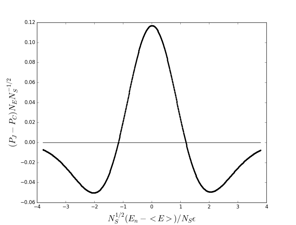
Figure 1: The scaled difference in the probabilities $(P_{J}-P_{C})N_{E}/N_{S}^{1/4}$ is plotted against the scaled system energies $N_{S}^{1/2}(E_{n}-\langle E\rangle)/N_{S}\epsilon$. The system contained $N_{S}=10^{4}$ SHO’s, while the environment contained $N_{S}=10^{4}$ SHO’s ($R=N_{S}/N_{E}=1$). The asymptotic behavior is shown, and the plot will not change for larger systems. The effective inverse temperature is $1.0$, and the average energy is $1.44$.

The scaling dependence of $\delta$ is then given by

$$\delta=\tilde{\delta}(N_{S}/N_{E})N_{S}^{3/4}N_{E}^{-1}$$ (26)

where $\tilde{\delta}(N_{S}/N_{E})$ is a function of the ratio $R=N_{S}/N_{E}$ for systems with either $N_{S}$ or $N_{E}$ larger than about $10^{4}$.

Table 2: The values of $\tilde{\delta}$ (the rescaled values of $\delta$) for a system of $N_{S}$ simple harmonic oscillators given in Eq. (20) from computations with environment composed of $N_{E}$ simple harmonic oscillators. The values of the system size, $N_{S}$, are given as headings of the columns. The average energy is $1.5$, and the temperature is $1.44$.

$N_{E}$	$10$	$10^{2}$	$10^{3}$	$10^{4}$	$10^{5}$	$10^{6}$
$10$	0.15314	0.06917	0.01507	0.00261	0.00046	0.00008
$10^{2}$	0.18610	0.14582	0.05795	0.01330	0.00255	0.00045
$10^{3}$	0.19155	0.18645	0.14472	0.05679	0.01287	0.00246
$10^{4}$	0.19215	0.19255	0.18649	0.14461	0.05666	0.01282
$10^{5}$	0.19221	0.19319	0.19266	0.18649	0.14459	0.05665
$10^{6}$	0.19221	0.19325	0.19331	0.19267	0.18649	0.14459

As an illustration, consider the following cases.

1. If the environment is much larger than the system ($N_{S}<<N_{E}$), then $\tilde{\delta}(R)$ becomes a constant as $R\rightarrow 0$, as seen in the bottom left side of Table 2.

2. For a fixed ratio $R=N_{S}/N_{E}$, $\delta\rightarrow N^{-1/4}$, as the sizes of the two systems increase (where $N$ is either $N_{S}$ or $N_{E}$). This can be seen by looking at any diagonal in Table 2, where the values of $\tilde{\delta}$ go to a constant. that depends on $R$. This decrease is rather slow, but the deviation from canonical behavior might still be hard to measure for a macroscopic system, as seen in Table 3.

   Table 3: The values of $\delta$ for $N_{S}=10^{20}$ as a function of the ratio $R=N_{S}/N_{E}$.

   $R$	$\delta$
   0.001	1.93E-9
   0.01	1.93E-8
   0.1	1.86E-7
   1	1.45E-6
   10	5.66E-6
   100	1.28E-5
   1000	2.46E-5

3. For the case that $N_{E}$ is large, $\tilde{\delta}$ is independent of $N_{S}$, and $\delta$ goes as $N_{S}^{3/4}$, as given by Eq. (26), and shown in Tables 1 and 2.

The numerical calculations have confirmed the predictions of Eq. (26).

V Comparison of canonical and joint distributions for the Ising model (second-order phase transitions)

The exchange of energy between an Ising model and a system of simple harmonic oscillators is different at the second-order phase transition and away from it. We will examine both cases.

V.1 Away from the second-order phase transition

We did calculations for an inverse temperature of $\beta=0.5$, which is well away from the critical value of $\beta_{c}=0.88137$. The energy was set as close to the average energy as possible, given the discrete spectrum.

To obtain a quantitative measure of the agreement, we compared a variety of sizes for both the system and the environment. The canonical distribution was used to obtain the best fit for the temperature. The deviation of the temperature from the desired value was small for all systems, and got dramatically smaller as the systems got larger. As can be seen from Tables 4 and 5, the data shows the same scaling given in Eq. (26).

Table 4: The values of $\delta$ for a system of $L\times L$ Ising models from computations with environment composed of $N_{E}$ simple harmonic oscillators. The values of the system size, $N_{S}=L^{2}$, are given as headings of the columns. The average energy is $-1.279$, and the inverse temperature is $\beta=0.5$.

$N_{E}$	$8\times 8$	$16\times 16$	$32\times 32$
$2^{6}$	2.05E-02	5.04E-02	9.69E-02
$2^{8}$	5.48E-03	1.46E-02	3.56E-02
$2^{10}$	1.40E-03	3.84E-03	1.04E-02
$2^{12}$	3.51E-04	9.72E-04	2.72E-03
$2^{14}$	8.79E-05	2.44E-04	6.88E-04
$2^{16}$	2.20E-05	6.10E-05	1.72E-04

Table 5: The values of $\tilde{\delta}$ (the rescaled values of $\delta$) for a system of $L\times L$ Ising models from computations with environment composed of $N_{E}$ simple harmonic oscillators. The values of the system size, $N_{S}=L^{2}$, are given as headings of the columns. The average energy is $-1.279$, and the inverse temperature is $\beta=0.5$.

$N_{E}$	$8\times 8$	$16\times 16$	$32\times 32$
$2^{6}$	0.05804	0.05044	0.03424
$2^{8}$	0.06197	0.05852	0.05033
$2^{10}$	0.06322	0.06139	0.05866
$2^{12}$	0.06359	0.06221	0.06146
$2^{14}$	0.06368	0.06244	0.06223
$2^{16}$	0.06369	0.06249	0.06227

V.2 At the second-order phase transition

The width of the peak in the energy is largest at the second-order phase transition due the connection between the variance of the energy and the specific heat.

$$c_{S}=C_{S}/N_{S}=\frac{1}{N_{S}k_{B}T^{2}}\left\langle\left(E-\langle E\rangle\right)^{2}\right\rangle$$ (27)

The increased width of the energy peak requires a larger environment to show a good approximation to the canonical ensemble. The improvement of the fit with increasing size is shown in Fig. 2.

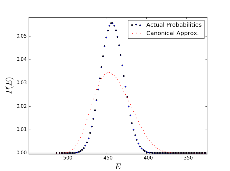
(a) $2^{8}$ SHO’s as environment.

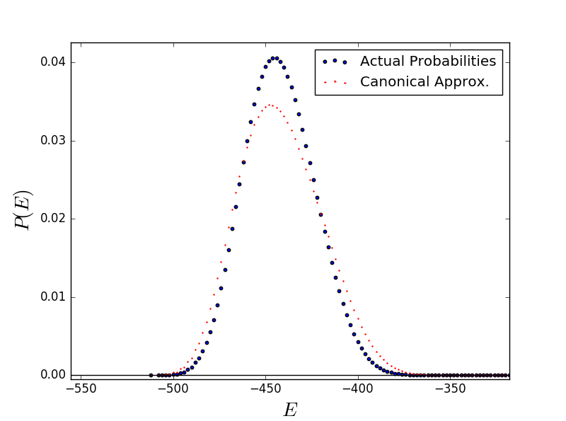
(b) $2^{10}$ SHO’s as environment.

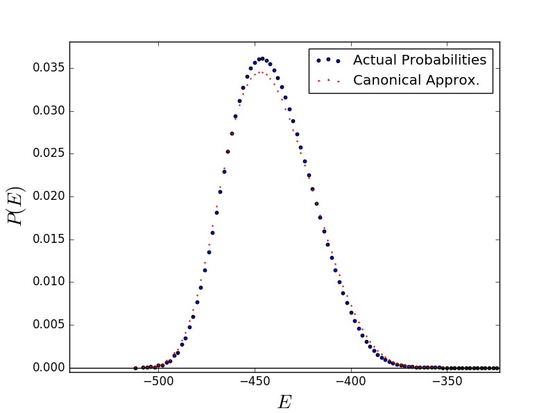
(c) $2^{12}$ SHO’s as environment..

Figure 2: Comparison of the canonical distribution (black dots) with the true joint distribution (red dots) for a Ising model on a $16\times 16$ lattice at the transition energy interacting with a system of simple harmonic oscillators. The system is at the critical inverse temperature.

The increase of the width of the critical energy peak also has the effect of increasing the value of $\delta$, which is shown in Table 6. The values should be compared to Table 4 for $\beta\neq\beta_{c}$, which are all smaller.

Table 6: The values of $\delta$ for a system of $L\times L$ Ising models from computations with environment composed of $N_{E}$ simple harmonic oscillators. The values of the system size, $N_{S}=L^{2}$, are given as headings of the columns. The temperature is $\beta_{c}=0.88137$.

$N_{E}$	$8\times 8$	$16\times 16$	$32\times 32$
$2^{6}$	1.00E-01	1.69E-01	2.14E-01
$2^{8}$	3.09E-02	7.46E-02	1.24E-01
$2^{10}$	8.18E-03	2.42E-02	5.73E-02
$2^{12}$	2.08E-03	6.58E-03	1.95E-02
$2^{14}$	5.21E-04	1.68E-03	5.42E-03
$2^{16}$	1.30E-04	4.22E-04	1.39E-03

We should be able to rescale $\delta$ for the Ising critical point to demonstrate the effect of the specific heat. Unfortunately, we have not been able to do this, probably because the systems are not large enough to show the asymptotic behavior.

VI Comparison of canonical and joint distributions for first-order transitions ($12$-state Potts model)

The twelve-state Potts model in two dimensions presents an interesting test of finite-canonical distributions. Away from the first-order transition, it shows the same finite-canonical behavior distribution as the system of simple harmonic oscillators seen in the previous section. At the first-order transition, the behavior is different.

In each case, the energy was chosen to correspond as closely as possible to the temperature being investigated ($\beta=1.0$ and $\beta_{c}=1.496068$). The value of the inverse temperature used for the comparison with the canonical distribution was then optimized to reduce the value of $\delta$. This temperature correction was about $1\%$ for the smallest example ($8\times 8$ Potts lattice and $64$ SHOs), but went down to $7.6\times 10^{-6}$ for a $32\times 32$ lattice and $N_{E}=2^{18}$.

We first demonstrate the behavior away from the transition.

VI.1 Away from the first-order transition

Values of $\delta$ were calculated for an inverse temperature of $\beta=1.0$, far from the first-order transition at $\beta_{c}=1.49607$. The scaled values for $\tilde{\delta}$ are given in Table 7. The patterns is the same as seen in Table 2, although the values of $\tilde{\delta}$ are somewhat smaller. The asymptotic scaling of $\delta$ is confirmed.

Table 7: The values of $\tilde{\delta}$ (the rescaled values of $\delta$) for a two-dimensional, $12$-state Potts model at $\beta\approx 1.0$ (away from the first-order transition). The size of the environment (a set of simple harmonic oscillators) is shown in the left column. Values of $\delta$ for the three sizes of the Potts model investigated ($8\times 8$, $16\times 16$, and $32\times 32$) are given in the next three columns.

$N_{E}$	$8\times 8$	$16\times 16$	$32\times 32$
$2^{6}$	0.10519	0.08274	0.04579
$2^{8}$	0.11993	0.11032	0.08200
$2^{10}$	0.12432	0.12291	0.11048
$2^{12}$	0.12556	0.12691	0.12289
$2^{14}$	0.12592	0.12803	0.12671
$2^{16}$	0.12599	0.13292	0.12769
$2^{18}$	0.12605	0.12837	0.12794

VI.2 At the first-order transition

For a first-order transition, the peak in the energy becomes a double peak with a distance between the two maxima that is proportional to the size of the system. The double peak structure at a first-order transition makes the analysis of this case differ for all others. For a small environment, the width of the distribution is dramatically limited, so that we see only a single peak, as shown in Fig. 3(a). As $N_{E}$ increases in Fig. 3(b) and 3(c), the full canonical distribution, with the double peak, emerges.

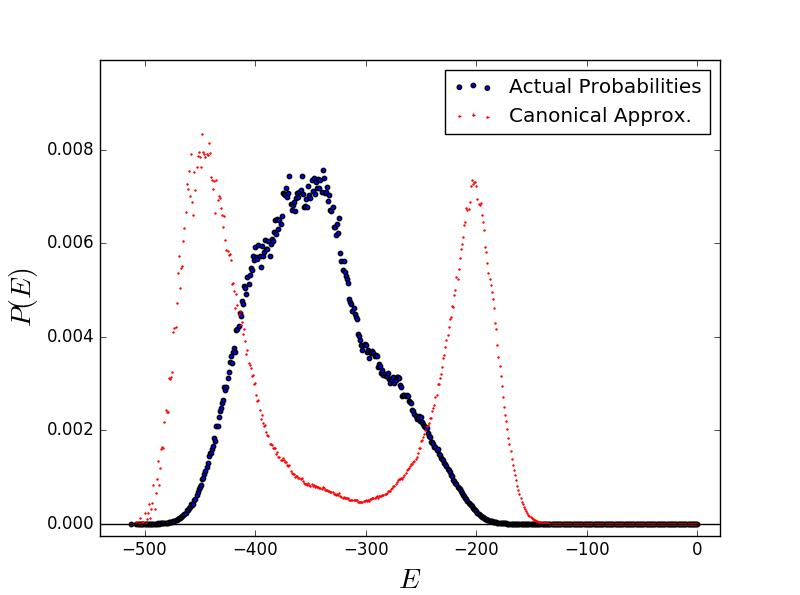
(a) $2^{12}$ simple harmonic oscillators.

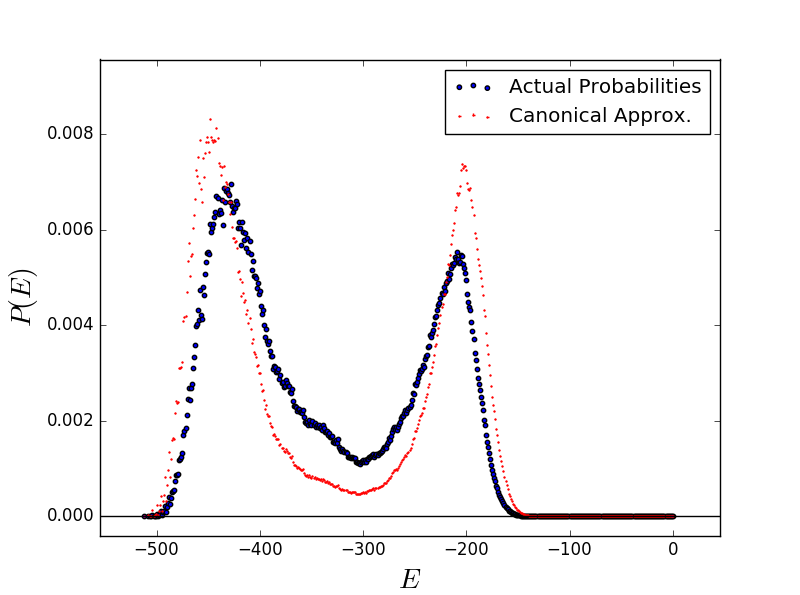
(b) $2^{14}$ simple harmonic oscillators.

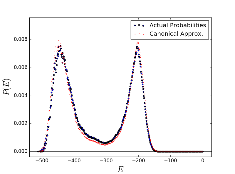
(c) $2^{16}$ simple harmonic oscillators.

Figure 3: Comparison of the canonical distribution (black dots) with the true joint distribution (red dots) for a $12$-states Potts model on a $16\times 16$ lattice at the energy of the phase transition interacting with a system of simple harmonic oscillators.

Table 8: The values of $\delta$ for a two-dimensional, $12$-state Potts model at $\beta_{c}$, the first-order transition. The size of the environment (a set of simple harmonic oscillators) is shown in the left column. Values of $\delta$ for the three sizes of the Potts model investigated ($8\times 8$, $16\times 16$, and $32\times 32$) are given in the next three columns.

$N_{E}$	$8\times 8$	$16\times 16$	$32\times 32$
$2^{6}$	2.367E-1	2.467E-1	2.474E-1
$2^{8}$	1.485E-1	1.800E-1	1.770E-1
$2^{10}$	6.106E-2	1.309E-1	1.280E-1
$2^{12}$	1.837E-2	7.995E-2	9.415E-2
$2^{14}$	4.868E-3	2.590E-2	6.801E-2
$2^{16}$	1.234E-3	6.567E-3	3.435E-2
$2^{18}$	3.096E-4	1.641E-3	9.576E-3
$2^{20}$	7.748E-5	4.100E-4	2.412E-3

Data for $\delta$ is shown in Table 8. The scaling of $\delta$ with $N_{E}^{-1}$ is satisfied. On the other hand, the scaling with the size of the system, $N_{S}$, is not even approximately satisfied. This is expected, because the width of the peak in the energy is not proportional to $N_{S}^{-1/2}$.

VII Conclusions

We have shown that the microcanonical ensemble, which assumes that the system of interest is in an energy eigenstate, does not give a correct description of an isolated system. If the history of the system includes any thermal contact with another system, it has a probability distribution that is spread over many eigenstates. With certain reasonable conditions on the sizes of the system of interest and the environment, the probability distribution is that of the canonical ensemble. This is true even when the “thermal reservoir” is 1000 times smaller than the system of interest.

At a second-order phase transition, the energy peak is wider than at a point away from the transition and the approach to the canonical ensemble with increased size is slower. However, a macroscopic system is still well described by the canonical distribution when the environment is substantially smaller than the system of interest.

For first-order transitions, the double-peak probability distribution requires the environment to be larger than the system, although still not infinite.

In all cases, the thermodynamic energy is a continuous variable, and the validity of the canonical ensemble does not require an infinite thermal reservoir.

References

- Boltzmann (1877) L. Boltzmann, “Über die Beziehung zwischen dem zweiten Hauptsatze der mechanischen Wärmetheorie und der Wahrscheinlichkeitsrechnung respektive den Sätzen über das Wärmegleichgewicht,” Wien. Ber., 76, 373–435 (1877), reprinted in Wissenschaftliche Abhandlungen von Ludwig Boltzmann (Chelsea, New York Vol. II, pp. 164-223.
- Sharp and Matschinsky (2015) K. Sharp and F. Matschinsky, “Translation of Ludwig Boltzmann’s paper on the relationship between the second fundamental theorem of the mechanical theory of heat and probability calculations regarding the conditions for thermal equilibrium, Sitzungberichte der Kaiserlichen Akademie der Wissenschaften. Mathematisch-Naturwissen Classe. abt. ii, lxxvi 1877, pp 373-435 (Wien. Ber. 1877, 76:373-435). reprinted in Wiss. Abhandlungen, vol. ii, reprint 42, p. 164-223, Barth, Leipzig, 1909,” Entropy, 17, 1971–2009 (2015), ISSN 1099-4300.
- Planck (1901) M. Planck, “Über das Gesetz der Energieverteilung im Normalspektrum,” Drudes Annalen, 553, 65–74 (1901), reprinted in Ostwalds Klassiker der exakten Wissenschaften, Band 206, “Die Ableitung der Strahlungsgesteze”.
- Callen (1985) H. B. Callen, Thermodynamics and an Introduction to Thermostatistics, 2nd ed. (Wiley, New York, 1985).
- Swendsen (2012) R. H. Swendsen, An Introduction to Statistical Mechanics and Thermodynamics (Oxford, London, 2012).
- Swendsen (2015) R. H. Swendsen, “Continuity of the entropy of macroscopic quantum systems,” Phys. Rev. E, 92, 052110 (2015).
- Jin et al. (2013) F. Jin, K. Michielsen, M. A. Novotny, S. Miyashita, S. Yuan, and H. De Raedt, “Quantum decoherence scaling with bath size: Importance of dynamics, connectivity, and randomness,” Phys. Rev. A, 87, 022117 (2013a).
- Jin et al. (2013) F. Jin, T. Neuhaus, K. Michielsen, S. Miyashita, M. A. Novotny, M. I. Katsnelson, and H. De Raedt, “Equilibration and thermalization of classical systems,” New Journal of Physics, 15, 033009 (2013b).
- Novotny et al. (2015) M.A. Novotny, F. Jin, S. Yuan, S. Miyashita, H. De Raedt, and K. Michielsen, “Quantum decoherence at finite temperatures,” (2015), arXiv:1502.03996v1 [cond-mat,stat-mech].
- Novotny et al. (2016) M. A. Novotny, F. Jin, S. Yuan, S. Miyashita, H. De Raedt, and K. Michielsen, “Quantum decoherence and thermalization at finite temperature within the canonical thermal state ensemble,” (2016), arXiv:1601.04209.