Studying Relation Between Star Formation and Molecular Clumps on Subparsec Scales in 30 Doradus

Abstract

We present $\mathrm{{}^{12}CO}$ and $\mathrm{{}^{13}CO}$ molecular gas data observed by ALMA, massive early stage young stellar objects identified by applying color-magnitude cuts to Spitzer and Herschel photometry, and low-mass late stage young stellar objects identified via H$\mathrm{\alpha}$ excess. Using dendrograms, we derive properties for the molecular cloud structures. This is the first time a dendrogram analysis has been applied to extragalactic clouds. The majority of clumps have a virial parameter equal to unity or less. The size-linewidth relations of $\mathrm{{}^{12}CO}$ and $\mathrm{{}^{13}CO}$ show the clumps in this study have a larger linewidth for a given size (by factor of 3.8 and 2.5, respectively) in comparison to several, but not all, previous studies. The larger linewidths in 30 Doradus compared to typical Milky Way quiescent clumps are probably due to the highly energetic environmental conditions of 30 Doradus. The slope of the size-linewidth relations of $\mathrm{{}^{12}CO}$, 0.65 $\pm$ 0.04, and $\mathrm{{}^{13}CO}$, 0.97 $\pm$ 0.12, are on the higher end but consistent within 3$\mathrm{\sigma}$ of previous studies. Massive star formation occurs in clumps with high masses ($\textgreater 1.83\times 10^{2}\;\mathrm{M_{\odot}}$), high linewidths (v $\textgreater 1.18\;\mathrm{km/s}$), and high mass densities ($\textgreater 6.67\times 10^{2}\;\mathrm{M_{\odot}\;pc^{-2}}$). The majority of embedded, massive young stellar objects are associated with a clump. However the majority of more evolved, low-mass young stellar objects are not associated with a clump.

Key Words: 30 Doradus, Molecular Clouds, Star Formation, YSOs

1 Introduction

1.1 Star Formation in the Large Magellanic Cloud

Massive stars have a profound impact on galaxies. Their great luminosities and intense ionizing radiation change the thermodynamic state of the surrounding interstellar medium (ISM) (Blake et al., 1987; Krause et al., 2013), their strong stellar winds compress the ISM (Lada, 1985; Heckman et al., 1990; Kudritzki & Puls, 2000; Hopkins et al., 2012), and their explosive ends enrich it with heavy elements (Woosley & Weaver, 1995; Woosley et al., 2002; Heger et al., 2003). Massive star formation is not a scaled up version of low-mass star formation. Formation of low-mass stars have been studied in detail within the Milky Way (e.g., Kroupa et al., 1993; Xue et al., 2008; Heiderman et al., 2010; Kafle et al., 2014). The intense radiation from high-mass stars has a significant effect on the surrounding medium as well as limits the accretion rate onto a high-mass protostar. Low-mass stars have very little gravitational effect on the surrounding gas or on other nearby stars. Massive stars play a more important role in defining the dynamics on the stellar cluster in which they reside: they can steal material from other stars (competitive accretion) (Tan et al., 2014). Massive stars have stellar winds and high ultraviolet radiation pressures that may trigger further star formation in nearby regions, which low-mass stars cannot do.

The Large Magellanic Cloud (LMC) provides an opportunity to study star formation at reduced metallicity of Z $\approx$ 0.5 $\mathrm{Z_{\odot}}$ (Westerlund, 1997). The nearly face-on viewing angle provides a unique view of resolved stellar populations without the confusion and extinction of the Galactic plane. Extinction to young stellar objects (YSOs) is nearly all associated with the star-forming region itself. Also, unlike in the Galaxy where distances are ambiguous, the distance to the LMC is well-determined (50 kpc, Feast (1999)), leading to robust luminosity determinations. The recent discoveries of thousands of YSO candidates in the LMC provides an opportunity to study massive star formation in both a statistical and detailed way (Meixner et al., 2006; Whitney et al., 2008; Seale et al., 2009; Chen et al., 2010; Carlson et al., 2012; Meixner et al., 2013; Seale et al., 2014). Fukui et al. (2015a) study previously identified YSO candidates in the N159 region of the LMC, and related the known YSO candidates to $\mathrm{{}^{12}CO}$ and $\mathrm{{}^{13}CO}$ ALMA observations of molecular gas. One of the young, massive YSO candidates in N159 is suspected to have formed via filamentary collision. Fukui et al. (2015b) look at two molecular clouds colliding in RCW 38, a young super star cluster in the Milky Way. The collision between two filaments in RCW 38 has lead to the formation of 20 O stars. Colliding filaments is one theory on how high-mass stars form. Another theory is based on competitive accretion. Star formation surveys show that the majority of low-mass, more evolved YSOs are found in clusters (Lada et al., 1993). Bonnell et al. (2001) simulate 100 stars in a cluster and find stars located at the centers of clusters accrete more gas than those at the outskirts. Competitive accretion is highly non-uniform and depends on the initial mass of the star as well as the star’s position in the cluster.

Previous observations, theories, and simulations all suggest the molecular gas structure is connected to the formation of high-mass stars (Goldbaum et al., 2011). In this paper we will discuss the impact of molecular gas and dust on massive star formation and make comments on how our results relate to previously observed thresholds necessary for high-mass star formation to occur.

1.2 Star Formation and Molecular Clumps in 30 Doradus

The 30 Doradus region, a.k.a. the Tarantula Nebula, provides a unique opportunity to study star formation over a range of masses and its feedback on the environment. 30 Doradus is one of the most active star formation regions in the Magellanic Clouds and the only Giant HII region in the Local group. At the heart of 30 Doradus is R136, the super star cluster with extraordinarily high stellar densities of $\textgreater 1.5\times 10^{4}-10^{7}\;\mathrm{M_{\odot}\;pc^{-3}}$ (Selman & Melnick, 2013), containing the most massive stars known (Crowther et al., 2010). Combining data from the Spitzer SAGE survey (Meixner et al., 2006), the Herschel Heritage survey (Meixner et al., 2013), and the Hubble Tarantula Treasury Project (HTTP) (Sabbi et al., 2013, 2016) we can study young and massive YSOs and low-mass and more evolved YSOs over the bulk of the mass function ($0.5-35\;\mathrm{M_{\odot}}$). Studying both low-mass and high-mass stars that are located in the same low-metallicity region can shed some light on the conditions necessary for star formation to occur.

The 30 Doradus region has been previously investigated in the tracers of the interstellar medium (ISM) that fuel the star formation. The dust content has been measured and quantified with the analysis of Spitzer SAGE (Meixner et al., 2006) and Herschel HERITAGE (Meixner et al., 2013) surveys by Gordon et al. (2014). $\mathrm{{}^{12}CO}$ (1-0) has been imaged as part of whole LMC surveys at $2.6^{\prime}$ with NANTEN (Fukui et al., 2008) and at $45^{\prime\prime}$ with MOPRA (Wong et al., 2011). $\mathrm{{}^{12}CO}$ (1-0), (2-1), and (3-2) have been observed in 30 Doradus by SEST (Johansson et al., 1998).

ALMA observations of $\mathrm{{}^{12}CO}$ (2-1), $\mathrm{{}^{13}CO}$ (2-1), and $\mathrm{C^{18}O}$ (2-1) clumps have been analyzed by Indebetouw et al. (2013). The $\mathrm{CO}$ observed in 30 Doradus is very clumpy, similar to that observed in the Milky Way. Analysis of the ALMA data shows a decrease in $\mathrm{{}^{12}CO}$ (2-1) emission relative to the total gas mass compared to massive star formation regions in the Milky Way, consistent with theory: there is less shielding in a lower-metallicity environment and $\mathrm{{}^{12}CO}$ (2-1) is not well shielded in comparison to $\mathrm{H_{2}}$ gas. High density gas tracers such as $\mathrm{HCN}$ (1-0) and $\mathrm{HCO^{+}}$ (1-0) show clumps in 30 Doradus have similar, but slightly larger linewidths than other regions in the LMC (Anderson et al., 2013). The physical conditions of the gas surrounding the R136 cluster have previously been constrained with ionized gas models (Indebetouw et al., 2009; Lopez et al., 2011; Pellegrini et al., 2011). Indebetouw et al. (2009) find photodissociated regions (PDRs) dominate over collisional excitation of shocks and that the effects of local hot stars play a more important role in shaping the gas chemistry than large scale trends with distance from the R136 cluster. The hot gas in 30 Doradus may be leaking out of the pores of the HII shells, since the X-ray gas pressure is measured to be much weaker than the radiation pressure (Lopez et al., 2011). $\mathrm{H_{2}}$ gas correlates well with $\mathrm{Br\gamma}$ and $\mathrm{CO}$ in the region, implying that the $\mathrm{H_{2}}$ gas comes from PDRs (Yeh et al., 2015). Further work on PDR modeling has been done by Chevance et al. (2016) who find 90$\%$ of [CII] emissions originates from PDRs and 70$\%$ of the far infrared luminosity is associated with the ionized gas component. Chevance et al. (2016) conclude that the gas in 30 Doradus is very porous and dominated by photoionization.

Our goal in this paper is to conduct a thorough investigation of early stage massive YSOs and later stage low-mass YSOs, and their relation to the clump structure of $\mathrm{{}^{12}CO}$ (2-1) and $\mathrm{{}^{13}CO}$ (2-1) molecular gas. This comprehensive study of high-mass and low-mass star formation with multi wavelength photometric and spectroscopic observations of molecular gas and dust will help shed light on the physical conditions necessary for high-mass star formation to take place. In Section 2 we describe the observations we use in more detail. In Section 3 we describe the dendrogram program we use to study the hierarchical structure of the clumps. In Section 4 we describe the YSOs in the study in more detail. In Section 5 we discuss the trends we see in molecular gas and how the how star formation is affected by the distribution of molecular gas. Lastly we present our conclusions in Section 6.

2 Observations

2.1 Spitzer Surveying the Agents of Galaxy Evolution (SAGE) and Herschel HERschel Inventory of the Agents of Galaxy Evolution (HERITAGE) Surveys

The SAGE survey imaged the LMC using IRAC (3.6 $\mu$m, 4.5 $\mu$m, 5.8 $\mu$m, 8.0 $\mu$m) and MIPS (24 $\mu$m, 70 $\mu$m, 160 $\mu$m) instruments on the Spitzer Space Telescope. One of the primary goals of the SAGE survey was to catalog YSOs in the LMC and study the current star formation rate in the LMC. The Herschel Heritage survey used the PACS and SPIRE instruments to image the LMC at 100 $\mu$m, 160 $\mu$m, 250 $\mu$m, 350 $\mu$m, 500 $\mu$m wavelengths in order to study the very cold dust surrounding the deeply embedded YSOs. Several YSO candidates we use in this work have previously been studied by Whitney et al. (2008); Gruendl & Chu (2009); Carlson et al. (2012); and Seale et al. (2014) who used the Spitzer SAGE (Meixner et al., 2006) and Herschel Heritage (Meixner et al., 2013) surveys.

2.2 Hubble Tarantula Treasury Project (HTTP)

HTTP is a survey of stellar populations in 30 Doradus that reaches into the sub-solar mass regime ($\textless 0.5\;\mathrm{M_{\odot}}$) (Sabbi et al., 2013, 2016). The survey includes optical (F555W and F658N with ACS and WFC), infrared (F110W and F160W with WFC3 and IR), and ultraviolet (F257W and F336W with WFC3 and UVIS). In addition, archival monochromatic survey in the F775W filter was used (realized using ACS/WFC and WFC3/UVIS in parallel). HTTP covers a projected area of 14’ x 12’ in the sky. We focus on the late-stage and more evolved YSOs (Sabbi et al., 2016) that are located within the 30 Doradus ALMA footprint (Indebetouw et al., 2013).

2.3 ALMA $\mathrm{{}^{12}CO}$ (2-1) and $\mathrm{{}^{13}CO}$ (2-1) Observation

ALMA allows us to resolve giant molecular clouds (GMCs) at the distance of the LMC with comparable resolution as HST, as well as provides us with high spectral resolution data. The frequency axis of the data is converted to velocity and results in a position-position-velocity (PPV) cube. The ALMA Cycle 0 footprint of 30 Doradus is a small region north of R136 and has been mapped with $\mathrm{{}^{12}CO}$ (2-1), $\mathrm{{}^{13}CO}$ (2-1), $\mathrm{C^{18}O}$, and $\mathrm{H30\alpha}$ (Indebetouw et al., 2013). Indebetouw et al. (2013) analyze the PPV data cubes and calculate mass, velocity, and size of the clumps. Figure  1 shows the HST F160W in greyscale, ALMA+APEX $\mathrm{{}^{13}CO}$ (2-1) in contour, and the location of the low-mass YSOs. Figure  1 shows the HST F160W in greyscale, ALMA+APEX $\mathrm{{}^{13}CO}$ (2-1) in contour, and the location of point sources from the SAGE catalog that are in the ALMA footprint. We use the ALMA Cycle 0 combined with APEX single dish observations of $\mathrm{{}^{12}CO}$ (2-1) and $\mathrm{{}^{13}CO}$ (2-1) made by Indebetouw et al. (2013) in our analysis.

3 Dendrogram Analysis

3.1 Astrophysical Motivation for Using Dendrogram Analysis

The molecular cloud structure determines where star formation occurs and the mass distribution of stars in a cluster. Molecular cloud sizes range several orders of magnitudes: high density parsec size clumps are nested within larger low density clumps that span several tens of parsecs (Lada, 1992). We use dendrograms as a way to study the hierarchical structure of the $\mathrm{{}^{12}CO}$ (2-1) and $\mathrm{{}^{13}CO}$ (2-1) emission from molecular clouds. We define clumps to mean any entity that is bound by an iso-intensity surface. Dendrogram algorithms look for the largest scale sizes first and then for smaller clumps embedded within the larger ones. This is different than previous studies which look at individual clumps and not nested structures. The dendrogram of a PPV data cube is a way to keep track of the iso-intensity surfaces over a range of size scales. If the intensities of a structure are not contiguous, then this structure is split into separate entities. The low-density gas is represented at the bottom of the hierarchical structure in a dendrogram, the starting branch of the structure. This branch connects to other branches and leaves that represent smaller and denser clumps embedded in the low-density media. The leaves and branches correspond to the different volumes in the data cube bounded by a given isosurface level.

Dendrogram analysis allows us to relate the low density ISM to the high density clumps in which star formation takes place. This novel approach is different than previous studies where a GMC would be separated into different clumps, however the structure as a whole would not be taken into account. Previous studies using dendrograms find that using this approach can lead to selecting GMCs in an automated way using only physically motivated criteria (Rosolowsky et al., 2008). Clumps in very active star forming regions like the central molecular zone (CMZ) follow the same size-linewidth relation slope as clumps in other Milky Way clouds but are offset higher by a certain factor (Shetty et al., 2012). Clumps with star formation tend to be more massive (for a given radius) than clumps without star formation (Kauffmann et al., 2010). With the use of dendrograms we can relate the parent clump (the starting branch of the dendrogram) to the child clumps (the leaves of the dendrogram) and study the contiguous nature that is inherent in the ISM.

3.2 Method

The astrodendro program uses what is known as the clipping method to calculate clump properties from a 2D image or a 3D data cube. The clipping method only accounts for emission above a contour level to be associated with an object, as oppose to extrapolating down to a zero intensity isosurface. The user has to input the minimum value to be considered in the data set, the threshold value that determines if a leaf will be a single entity or not, and the minimum number of pixels for a leaf to be considered a single entity. The larger branch breaks down into leaves depending on the three input criteria. Figure  2 a shows the dendrogram structure of $\mathrm{{}^{13}CO}$ (2-1) column density, Figure  2 b shows how the dendrogram structure relates to the molecular clouds. Figure  3 a shows the $\mathrm{{}^{12}CO}$ (2-1) brightness temperature, Figure  3 b shows the corresponding emission map. The individual dendrogram structures of $\mathrm{{}^{13}CO}$ (2-1) and $\mathrm{{}^{12}CO}$ (2-1) are different because we are looking at two different quantities (column density and brightness temperature) and because of optical depth effects. The dendrogram structures highlighted in Figures  2 b and  3 b were chosen in order to illustrate how branches and leaves translate to an image map. The astrodendro program outputs the total integrated luminosity of an isosurface (a.k.a. clump), the linewidth ($\mathrm{v_{RMS}}$) of the clump, and the area of the clump, the effective radius of the clump, and the orientation angle of the clump. These properties can be used to calculate relevant astrophysical properties such as the column density or mass.

3.3 Results from Dendrogram Analysis of $\mathrm{{}^{12}CO}$ (2-1) and $\mathrm{{}^{13}CO}$ (2-1) Emission in 30 Doradus

The most dominant molecular species in the ISM is $\mathrm{H_{2}}$. Unfortunately $\mathrm{H_{2}}$ does not have any dipole moment, all of the low energy transitions are quadrupole transitions with small transition probabilities and high excitation energies. This means that the $\mathrm{H_{2}}$ is excited at high temperatures or in the vicinity of strong ultraviolet radiation. The most abundant molecule in the ISM is invisible to direct observation since the majority of ISM conditions cannot excite it. The second most abundant molecule in the ISM is CO and is frequently used to estimate the $\mathrm{H_{2}}$ gas mass via a conversion factor. Leroy et al. (2011) find the $\mathrm{{}^{12}CO-to-H_{2}}$ conversion factor (or the X-factor) in the LMC to be $3-9\;\mathrm{M_{\odot}\;pc^{-2}\;(K\;km\;s^{-1})^{-1}}$ in the local group which includes: M21, M33, the LMC, NGC 6822, and the SMC. The $\mathrm{M_{mol}}$/F($\mathrm{{}^{12}CO}\;1-0$) X-factor of 30 Doradus is higher than the average X-factor in the LMC: Indebetouw et al. (2013) compare the calculated molecular mass to the $\mathrm{{}^{12}CO}$ (2-1) intensity and find that the X-factor is $12\pm 4\;\mathrm{M_{\odot}\;pc^{-2}\;(K\;km\;s^{-1})^{-1}}$. We calculate the brightness temperature integrated over the velocity for $\mathrm{{}^{12}CO}$ (2-1) and use a X-factor of $12\pm 4\;\mathrm{M_{\odot}\;pc^{-2}\;(K\;km\;s^{-1})^{-1}}$. The total mass of all dendrogram branches in Figure  3 a is $1.3\pm 0.4\times 10^{5}\;\mathrm{M_{\odot}}$. Table 1 lists the mass of the $\mathrm{{}^{12}CO}$ (2-1) clumps.

Table 2 lists column density and mass values we obtain on the $\mathrm{{}^{13}CO}$ (2-1) clumps. The equations we used to convert the $\mathrm{{}^{13}CO}$ (2-1) column density to the $\mathrm{H_{2}}$ mass can be found in Appendix A. We use a $\mathrm{H_{2}/^{13}CO}$ abundance ratio of $5\times 10^{6}$ to convert the $\mathrm{{}^{13}CO}$ column density to the $\mathrm{H_{2}}$ column density, the same abundance factor that was used by Indebetouw et al. (2013). The total $\mathrm{H_{2}}$ mass we obtain by summing up the masses of each dendrogram trunk in Figure  2 a is $6.7\times 10^{4}\;\mathrm{M_{\odot}}$. The mass estimated from $\mathrm{{}^{13}CO}$ (2-1) and $\mathrm{{}^{12}CO}$ (2-1) in this work are consistent with each other as well as those estimated by Indebetouw et al. (2013) using dust continuum emission ($6.0\pm 1.0\times 10^{4}\;\mathrm{M_{\odot}}$) and LTE analysis of $\mathrm{{}^{13}CO}$ (2-1) ($6.8\times 10^{4}\;\mathrm{M_{\odot}}$).

4 Massive YSOs and Low-Mass YSOs

The molecular clump sizes range from 0.2 - 1.4 $\mathrm{pc}$. To trace star formation at this scale we need an inventory of the forming stars. We use recent surveys (HTTP, Spitzer SAGE, Herschel HERITAGE) to make a catalog of all the low-mass and massive YSOs. We define the stage of the YSO candidates in our sample by the following: Stage 0/I objects have $\mathrm{\frac{{\dot{M}_{env}}}{M_{star}}}\textgreater 10^{-6}\;\mathrm{yr^{-1}}$, Stage II objects are those that have $\mathrm{\frac{{\dot{M}_{env}}}{M_{star}}}\textless 10^{-6}\;\mathrm{yr^{-1}}$ and $\mathrm{\frac{M_{disk}}{M_{star}}}\textgreater 10^{-6}$, and Stage III objects have $\mathrm{\frac{{\dot{M}_{env}}}{M_{star}}}\textless 10^{-6}\;\mathrm{yr^{-1}}$ and $\mathrm{\frac{M_{disk}}{M_{star}}}\textless 10^{-6}$ (Robitaille et al., 2006, 2007; Chen et al., 2010).

4.1 Stage III Low-Mass YSOs

Stage III low-mass YSOs are usually identified by their location in an optical color-magnitude diagram, which leads to two problems: 1) contamination by older field stars and the effects of differential extinction that may lead to an overestimate of the actual number of candidates 2) older YSOs that are close to the main sequence (MS) cannot be identified accurately (De Marchi et al., 2011c). An alternate method of looking for Stage III low-mass YSOs is by H$\mathrm{\alpha}$ excess from accretion shocks (De Marchi et al., 2011c). Strong and fast variability of the H$\mathrm{\alpha}$ line intensity has been detected spectroscopically (e.g., Fernandez et al., 1995; Reipurth et al., 1996; Smith et al., 1999; Alencar et al., 2001, 2005; Sousa et al., 2016) that can move a star above and below our 10 Angstrom equivalent width threshold in a few days and sometimes in a few hours. Comparing observations of the SN 1987A field taken at 3 different epochs (Romaniello, 1998; Panagia et al., 2000) revealed that the number of stars that have strong H$\mathrm{\alpha}$ excess is essentially the same at all epochs, but only about about 1/3 of them are that strong at all epochs. This suggests a duty cycle of about 1/3. An ongoing study of the PMS stars in NGC 346, based on the original work of De Marchi et al. (2011b, a) revealed that the number of H$\mathrm{\alpha}$ strong PMS stars in the ‘classical’ region of the color magnitude diagram (CMD) (i.e. stars brighter and redder than the MS) are between 1/3 and 2/3 of all the stars in the same region (De Marchi $\&$ Panagia, private communication). Note that in the case of NGC 346 the reddening is not so high ($\mathrm{A_{v}}\approx 0.5$) and, therefore, there is no serious problem of contamination in that region of the CMD. All those elements taken together suggest that the duty cycle of relatively young PMS stars (those still above and redder than the MS) should be of the order of 1/3.

We have used the HTTP catalog (Sabbi et al., 2016) to select the low-mass Stage III YSO candidates with H$\mathrm{\alpha}$ excess within the ALMA footprint using the stringent selection criteria as defined by De Marchi et al. (2011c). In particular, all selected stars must have uncertainties lower than 0.1 mag in each of the V, I and H$\mathrm{\alpha}$ bands, simultaneously. Furthermore, they must display V-H$\mathrm{\alpha}$ excesses higher than the 4$\mathrm{\sigma}$ level as compared to stars of the same V-I color. There are 87 stars that meet the above criteria and are located within the ALMA footprint.

Figures  4 a and  4 b shows the F160W versus F110W - F160W color-magnitude diagram (CMD) with isochrones and mass evolutionary tracks overplotted. We plot isochrones and mass evolutionary tracks taken from the Padova code (Bressan et al., 2012; Chen et al., 2015) on these figures. For our purposes we use Milky Way extinction of $\mathrm{A_{v}}=0.06$ and metallicity of $\mathrm{Z}=0.008$ to redden the Padova isochrones to their location in the LMC. In addition we use the local extinction of 30 Doradus as calculated by De Marchi et al. (2016) to de-redden the low-mass YSOs. The majority of stars fall between $10^{5}-10^{7}\;\mathrm{yrs}$ isochrones and $1-3\;\mathrm{M_{\odot}}$ mass evolutionary tracks. Table 3 lists the approximate masses of these low-mass YSOs. These masses were calculated by the best fit mass evolutionary track from F160W versus F110W - F160W for each source. When we check these mass estimates with the best fit mass evolutionary track to F775W versus F555W - F775W for each source, we find that 75$\%$ of the masses do not match. The masses from the best fit evolutionary track to F775W versus F555W - F775W are always lower than those from F160W versus F110W - F160W. We choose the near infrared CMD mass evolution tracks to determine the mass because these wavelengths are not as contaminated from extinction as optical bands. All masses of low-mass YSOs have an uncertainty of $\pm 0.25\;\mathrm{M_{\odot}}$. This is due to the the $0.5\;\mathrm{M_{\odot}}$ spacing between the mass evolutionary track (Figure  4 b).

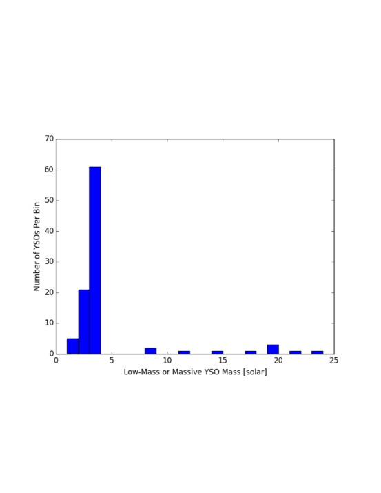
Figure 7: Mass distribution of low-mass and massive YSOs.

We are not complete in our catalog of low-mass YSOs due to the H$\mathrm{\alpha}$ duty cycle - selection of low-mass YSOs by H$\mathrm{\alpha}$ excess means at any given time we can observe 1/3 of the stars. Selecting the low-mass YSOs by H$\mathrm{\alpha}$ excess means that we are targeting Stage III objects. Figure  7 shows a histogram of all massive and low-mass YSO star masses. The majority of low-mass YSOs in our analysis are $3\;\mathrm{M_{\odot}}$. We do not select any Stage I or Stage II low-mass YSO candidates. This is the result of our bias towards selecting low-mass Stage III YSOs by H$\mathrm{\alpha}$ excess.

4.2 Stage I Massive YSOs

4.2.1 Overview

We include massive YSO stage I candidates found by Gruendl & Chu (2009) and Seale et al. (2009, 2014) in our study. There are no massive stage I YSO candidates from Whitney et al. (2008) that are found in the ALMA CO footprint. Gruendl & Chu (2009); Whitney et al. (2008) implements color cuts of different kinds, Seale et al. (2009) was a spectroscopic follow-up of Gruendl & Chu (2009) sources, and Walborn et al. (2013) study 10 Spitzer selected YSOs in 30 Doradus in more detail in order to provide mass estimates of these objects. Seale et al. (2009) use Spitzer IRS spectra and group YSO candidates in six categories. The S Group objects have silicate absorption features including the 10 $\mu$m absorption feature and sometimes including the 18 $\mu$m absorption feature, the SE Group objects have both silicate absorption features (similar to S Group) and strong fine-structure emission lines, the P group objects have strong PAH features, the PE group objects have strong PAH and fine-structure line emission, the E group contain sources that only have very strong fine-structure emission lines, and the F group all other sources whose spectra looks similar to that of a YSO but they do not fit any of the above criteria.

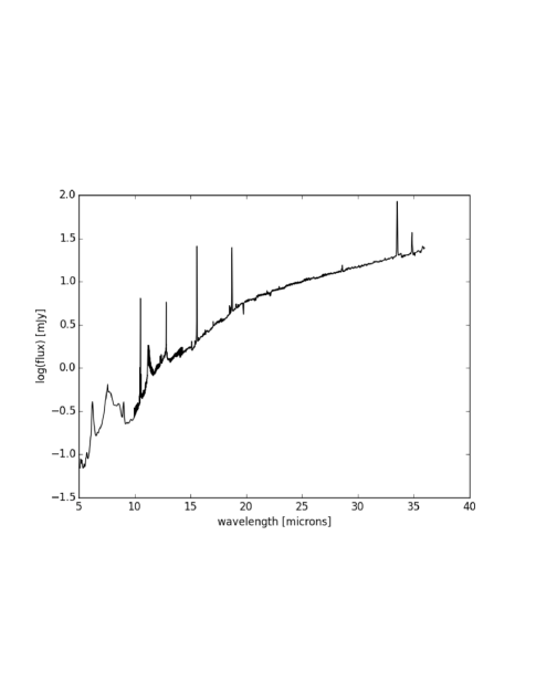
(a)

(b)

(c)

Figure 6: Spectra of YSO candidates in the 30 Doradus ALMA footprint. Left: J84.703995-69.079110. Center: J84.688990-69.084695 . Right: J84.720292-69.077084. Prominent features include PAH (6.2 $\mu$m), PAH (7.7 $\mu$m), PAH (8.6 $\mu$m), [ArIII] (8.99 $\mu$m), silicon absorption (9.7 $\mu$m), $\mathrm{H_{2}}$ (9.7 $\mu$m), [SIV] (10.5 $\mu$m), PAH (11.2 $\mu$m), $\mathrm{H_{2}}$ (12.3 $\mu$m), [NeII] (12.81 $\mu$m), [NeII] (15.55 $\mu$m), $\mathrm{H_{2}}$ (17.1 $\mu$m), [SIII] (18.71 $\mu$m), [SIII] (33.48 $\mu$m), and [SiII] (34.81 $\mu$m).

We look at all point source objects in the SAGE catalog that are in the ALMA footprint of 30 Doradus to see if any possible massive YSO candidates were missed by previous galaxy wide studies because of stringent cuts. There are 6 YSO candidates that have previously been identified: J84.703995-69.079110, J84.699755-69.069803, J84.688990-69.084695, J84.695173-69.084857, J84.726173-69.082254, and J84.720292-69.077084. And there are 9 point sources in the ALMA footprint that have not been studied before: J84.695932-69.083807, J84.688372-69.078168, J84.669113-69.081638, J84.674734-69.077374, J84.709403-69.075682, J84.688168-69.071013, J84.694286-69.074499, J84.676469-69.082774, and J84.671132-69.077168. We fit these sources to the Robitaille et al. (2006, 2007) spectral energy distribution (SED) fitter. We develop a code which we use in conjunction with the Robitaille et al. (2006) SED fitter. This code outputs the maximum likelihood of the YSO parameters such as mass, luminosity, accretion rate, and associated 1$\mathrm{\sigma}$ errors. Tables 4 and 5 list the near infrared and far infrared photometry we used. For candidates with no PACS or SPIRE photometry we use the upper limit in each far infrared band as given in Table 6 of Meixner et al. (2013). We assume the 6 previously identified YSO candidates are real candidates. For the 9 new point sources in the Spitzer footprint that have not been previously studied we require the reduced $\mathrm{\chi^{2}}$ of the best fit YSO SED to be less than 10 and the reduced $\mathrm{\chi^{2}}$ of the best fit stellar photosphere to be greater than 10. If an object is a good match to a YSO SED and not a good match to a reddened stellar photosphere SED, then we say it is a YSO candidate. With this definition we identify 4 new YSO candidates: J84.695932-69.083807, J84.688372-69.078168, J84.669113-69.081638, and J84.674734-69.077374. There are 5 Spitzer point sources that do not meet our $\mathrm{\chi^{2}}$ criteria: J84.709403-69.075682, J84.688168-69.071013, J84.694286-69.074499, J84.676469-69.082774 and J84.671132-69.077168. We look at the $\mathrm{{}^{12}CO}$ (2-1) map and find that the emission at the location of these 5 sources is less than $3\mathrm{\sigma}$. Figures  5 shows SEDs of all YSO candidates. Figure  6 shows spectra for 3 massive YSO candidates.

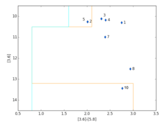
Figure 8: CMD of IRAC [3.6] versus IRAC [3.6] - IRAC [5.8]. Everything to the right of the orange line fits the criteria for the Carlson et al. (2012) $\mathrm{\alpha}$ cut and everything to the right of the cyan line fits the Carlson et al. (2012) $\mathrm{\beta}$ cut. Numbers next to each point correspond to the rank of the YSO candidates from most massive to least massive as listed in Table 6. Even though we have a total of 11 YSO candidates, we only have 8 objects plotted because a few of them are missing [3.6] or [5.8] photometry.

Carlson et al. (2012) also used multi-color cuts, but included more of a grey zone with $\mathrm{\alpha}$ and $\mathrm{\beta}$ cuts to include bluer sources at a lower reliability in comparison to Gruendl & Chu (2009). The Carlson et al. (2012) cuts are based on Spitzer IRAC (3.6 $\mu$m, 4.5 $\mu$m, 5.8 $\mu$m, 8.0 $\mu$m) and MIPS (24 $\mu$m) color-magnitude diagrams (CMDs). The $\mathrm{\alpha}$ cut criteria can be applied to galaxy-wide surveys and has a low contamination rate. Applying $\mathrm{\alpha}$ cuts selects the most massive and luminous YSOs. The $\mathrm{\beta}$ cut criteria should be applied to star-forming regions with less contamination from background sources, where it is more likely the cuts will select a YSO. Figure  8 shows [3.6] versus [3.5]-[5.8] CMD. YSO candidates numbered 1, 3, 4, and 7 have been previously studied (Gruendl & Chu, 2009; Seale et al., 2009, 2014). These four YSO candidates meet the Carlson et al. (2012) $\mathrm{\alpha}$ cut criteria (all located to the right of the orange line). YSO candidates 2, 5, 8, and 10 have not been previously identified. YSO candidate 8 meets the Carlson et al. (2012) $\mathrm{\alpha}$ cut criteria. YSO candidates 2, 5, and 10 meet the Carlson et al. (2012) $\mathrm{\beta}$ cut criteria. The YSO numbering refers to ranking from most massive to least massive YSO, as given in Table 6.

The 6 previously identified YSO candidates and the 4 new YSO candidates in this work are all Stage I objects as given by the peak of the likelihood distribution of $\mathrm{\frac{\dot{M_{env}}}{M_{star}}}$. Our goal is to find out how massive star formation relates to molecular clumps. Even though we are most likely missing many later stage low-mass YSOs, our catalog of massive Stage I YSO candidates (objects $\textgreater 8\;\mathrm{M_{\odot}}$ in Figure  7) is complete.

In addition to Stage, we can characterize the SED by Type. Chen et al. (2010) conduct an empirical analysis by looking at the shape of the SEDs to classify it by Type: Type I YSOs have SEDs with a steady rise in the near infrared and a high peak at 8-24 $\mu$m, Type II YSOs have low peak in the optical and a peak in the near infrared as well, Type III have SEDs peaking in the optical with some peak in the near or mid infrared wavelengths. There is correlation between Type I and Stage I YSOs, because these objects are deeply embedding within a molecular cloud. However there is little to no correlation between the any other Type and Stage classification. Below we list each of the YSO candidates in this study and describe the SED morphology in more detail.

4.2.2 Details of Each YSO Candidate in Order of Most Massive to Least Massive

J84.703995-69.079110: This massive YSO candidate in our work is located in the central, most massive clump as can be seen in Figure  1. The spectra for this source is shown in the top panel of Figure  6. This YSO candidate is in the PE group (Seale et al., 2009). There is a silicon absorption feature visible, as well as strong PAH and fine-structure line emission. There is a steep rise in the SED as shown in Figure  5, and a peak in the mid infrared. This object is a Type I YSO. This object also meets one of the Carlson et al. (2012) $\mathrm{\alpha}$ cut criteria. Walborn et al. (2013) find there are two water masers associated with this object and the spectral type of the object is O2.

J84.695932-69.083807: This second most massive YSO candidate is located in clump 13 ($\mathrm{{}^{13}CO}$ (2-1) clump as listed in Table 1), as well as clumps 14 and 25. This object also meets one of the Carlson et al. (2012) $\mathrm{\beta}$ cut criteria. There is a shallow rise from the near infrared to the far infrared wavelengths in the SED, therefore we say this is a Type II YSO. This object along with J84.695173-69.084857 is a double source and labeled as IRSN 122 and IRSN 126 by Rubio et al. (1998).

J84.699755-69.069803: The SED of the YSO candidate shows a steep rise in the IRAC bands, therefore we say this is a Type I YSO. This object also meets one of the Carlson et al. (2012) $\mathrm{\alpha}$ cut criteria. Walborn et al. (2013) find this object to be a bright source surrounded by a cluster of faint sources, and the entire cluster is surrounded by a thick annulus of emission in the Spitzer/MIPS 24$\mathrm{\mu m}$ image.

J84.688990-69.084695: Seale et al. (2009) categorize this object to be in the PE group. The spectra is shown in the central panel of Figure  6. There is no silicon absorption feature, however there are strong PAH and fine-structure line emission features. A lack of silicon absorption may mean this candidate is more evolved that the other two YSO candidates that have spectra in our work(J84.703995-69.079110 and J84.720292-69.077084). This YSO candidate is located inside clump 8 ($\mathrm{{}^{13}CO}$ (2-1) clump as listed in Table 1). There is a double peak in the SED of this object, with one peak in the near infrared and the other peak in the far infrared. Therefore we classify this objects as a Type II YSO candidate. his object also meets one of the Carlson et al. (2012) $\mathrm{\alpha}$ cut criteria.

J84.695173-69.084857: This YSO candidate is located inside clump 15 ($\mathrm{{}^{13}CO}$ (2-1) clump as listed in Table 1). This object meets Carlson et al. (2012) $\mathrm{\alpha}$ and $\mathrm{\beta}$ cut criteria. There is a shallow rise from the near infrared to the far infrared wavelengths in the SED, therefore we say this is a Type II YSO. This object and J84.695932-69.083807 are part of a double source as studied by Walborn et al. (2013).

J84.726173-69.082254: The SED of the YSO candidate shows a steep rise in the IRAC bands, therefore we say this is a Type I YSO.

J84.720292-69.077084: This object is in the PE group (Seale et al., 2009). The spectra shown in the bottom panel of Figure  6 shown silicon absorption, PAH emission, and fine-structure line emission. This YSO candidate is located inside clump 9 ($\mathrm{{}^{13}CO}$ (2-1) clump as listed in Table 1). There is a steep rise in the SED as shown in Figure  5, and a peak in the far infrared. This object is a Type I YSO. This objects meets Carlson et al. (2012) $\mathrm{\alpha}$ cut criteria. Walborn et al. (2013) find a water maser near this object.

J84.688372-69.078168: This YSO candidate is located within $\mathrm{{}^{13}CO}$ (2-1) clumps 29 and 30. This object also meets one of the Carlson et al. (2012) $\mathrm{\alpha}$ cut criteria. This YSO is Type I YSO due to the prominent peak of the SED in mid infrared wavelengths. There is a steep rise in the SED as shown in Figure  5, and a peak in the far infrared. This object is a Type I YSO.

J84.669113-69.081638:This YSO candidate is located within $\mathrm{{}^{13}CO}$ (2-1) clump 46 and meets one of the Carlson et al. (2012) $\mathrm{\alpha}$ cut criteria. This object is a Type III YSO candidate due to the similar strength of the near infrared and far infrared peaks in the SED.

J84.674734-69.077374: This object meets the Carlson et al. (2012) $\mathrm{\alpha}$ and $\mathrm{\beta}$ cut criteria. This object is a Type III YSO candidate due to the similar strength of the near infrared and far infrared peak in the SED.

5 Results and Discussion

5.1 Size, Linewidth, and Mass Surface Density

The ‘universality’ of Larson’s law has been verified by other observations (Lada, 1985; Bolatto et al., 2008; Heyer et al., 2009) and simulations (Federrath & Klessen, 2012; Goldbaum et al., 2011). Shetty et al. (2012) study the central molecular zone (CMZ) and analyze $\mathrm{N_{2}H^{+}}$, $\mathrm{HCN}$, $\mathrm{H^{13}CN}$, and $\mathrm{HCO^{+}}$ using dendrograms. They find a slope of 0.67, 0.46, 0.78, 0.64 and a coefficient of 2.6, 3.8, 2.6, 2.1 for $\mathrm{N_{2}H^{+}}$, $\mathrm{HCN}$, $\mathrm{H^{13}CN}$, and $\mathrm{HCO^{+}}$ respectively. There is a similarity in the slope of the size-linewidth relation that is independent of the local environmental factors and independent of the particular molecular gas that is studied. Bolatto et al. (2008) find the slope to be 0.60 in extra-galactic clouds, Heyer et al. (2009) find the slope to be 0.50 in Milky Way clouds, Shetty et al. (2012) find the slope to range between 0.46 and 0.78 in the CMZ for several high density tracers. This agreement in the slope of the size-linewidth relation is theorized to be because of the universality of turbulence (Heyer & Brunt, 2004).

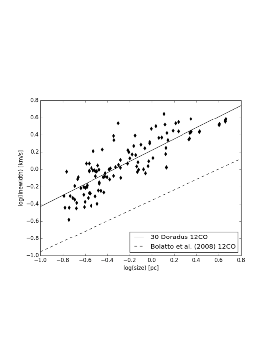
Figure 9: Size-linewidth relation of $\mathrm{{}^{12}CO}$ (2-1) brightness temperature clumps. The best fit line is given by $\mathrm{\sigma=(1.66\pm 0.06)r^{(0.65\pm 0.04)}}$. The dashed line, given by the equation $\mathrm{\sigma=0.44r^{0.60}}$, is the best-fit line for extragalactic $\mathrm{{}^{12}CO}$ molecular cloud analyzed by Bolatto et al. (2008). The $\mathrm{{}^{12}CO}$ (2-1) linewidths of clumps in 30 Doradus are offset from extragalactic clumps by a factor of 3.8.

Figure  9 shows the corresponding size-linewidth relation of the $\mathrm{{}^{12}CO(2-1)}$ brightness temperature clumps. In order to define a radius we use the geometric mean of the major axis radius and minor axis radius of the best-fit ellipse to the clump. The best fit line to the $\mathrm{{}^{12}CO}$ (2-1) clumps in this study is given by the equation $\mathrm{\sigma=(1.66\pm 0.06)r^{(0.65\pm 0.04)}}$. We find the slope of the $\mathrm{{}^{12}CO}$ (2-1) size-linewidth relation to be similar to extragalactic clouds studied by Bolatto et al. (2008), but the clumps in this 30 Doradus study have a systematic offset to larger linewidths by a factor of 3.8.

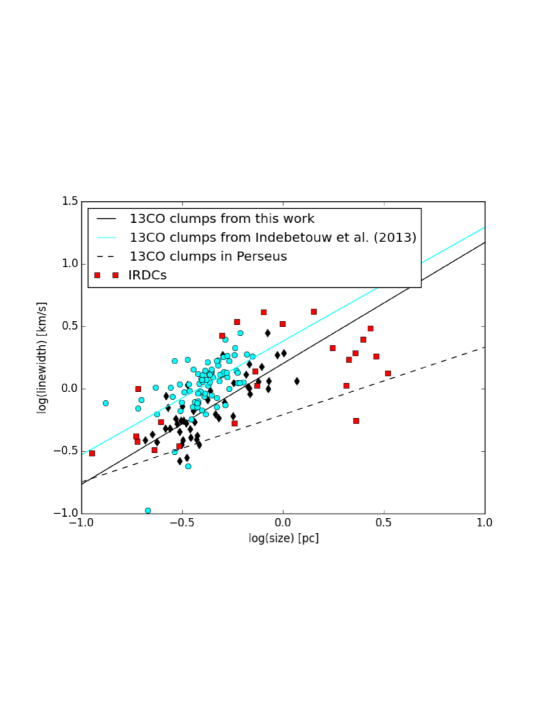
Figure 10: The size (of astrodendro clumps and cprops clumps) is calculated from the weighted second moment in two spatial directions, specifically the direction of greatest spatial extent and perpendicular to that. The radius is then 1.91 times the geometric mean of those two spatial second moments. The linewidth is calculated using the weighted velocity second moment of the pixels assigned to the cprops clump or astrodendro structure. Black diamonds are the size-linewidth values of $\mathrm{{}^{13}CO}$ (2-1) clumps in this study. The best fit line of astrodendro clumps is given by the equation $\mathrm{\sigma=(1.58\pm 0.18)r^{(0.97\pm 0.12)}}$ and represented by the solid black line. Cyan circles are 30 Doradus $\mathrm{{}^{13}CO}$ (2-1) brightness temperature size-linewidth clumps from Indebetouw et al. (2013). The Indebetouw et al. (2013) clumps are systematically offset by the clumps in this work by a factor of 1.5. This difference is because astrodendro systematically calculates smaller linewidths for clumps that are comparable in size to the clumps found by cprops. See Appendix B for further details. The best fit line of the cprops clumps is given by the equation $\mathrm{\sigma=(2.39\pm 0.33)r^{(0.91\pm 0.15)}}$ and represented by the solid cyan line. Red squares are size-linewidths from infrared dark cloud studies by Gibson et al. (2009); Bontemps et al. (2010); Peretto et al. (2013). We converted the FWHM to $\sigma$ by dividing the FWHM values given in the infrared dark cloud studies by a factor of 2.35. The dashed line ($\mathrm{\sigma=0.62r^{0.54}}$) is the best-fit line for molecular clumps in Perseus analysis by Shetty et al. (2012) using dendrograms. The 30 Doradus clumps are offset from the Perseus clumps by a factor of 2.5.

Figure  10 shows the size-linewidth of $\mathrm{{}^{13}CO(2-1)}$ clumps analyzed using dendrograms and $\mathrm{{}^{13}CO(2-1)}$ clumps analyzed by Indebetouw et al. (2013) using cprops Rosolowsky & Leroy (2006). The astrodendro algorithm calculated smaller linewidths for a given clump size. This can be seen in Figure  10 and is further explained in Appendix B: the astrodendro clumps have smaller linewidth for a given size. The best-fit line for the $\mathrm{{}^{13}CO(2-1)}$ clumps from this study is given by the solid black line ($\mathrm{\sigma=(1.58\pm 0.18)r^{(0.97\pm 0.12)}}$). The best-fit line for the $\mathrm{{}^{13}CO(2-1)}$ clumps from (Indebetouw et al., 2013) is given by the solid cyan line ($\mathrm{\sigma=(2.39\pm 0.33)r^{(0.91\pm 0.15)}}$). The cyan points in Figure  10 use the same regions in position-position-velocity (PPV) space as the clumps defined using cprops and analyzed in (Indebetouw et al., 2013), but a different method to calculate size and linewidth, to be more consistent with the astrodentro calculation. In this paper we use the same definition of size for both astrodendro clumps and cprops clumps. The size is calculated from the weighted second moment in two spatial directions. The radius is 1.91 times the geometric mean of those two spatial second moments (Solomon et al., 1987). The linewidth is calculated using the weighted velocity second moment of the pixels assigned to the cprops clump or astrodendro structure. More details of the sizes and linewidths from cprops and astrodendro can be found in Appendix C. The analysis in this work is in agreement with Indebetouw et al. (2013): the $\mathrm{{}^{13}CO(2-1)}$ clumps derived from astrodendro lie in the same parameter space as the clumps analyzed by cprops (Indebetouw et al., 2013).

One comparable analysis to our work in that of the Perseus cloud in the Milky Way by Shetty et al. (2012). The dashed line in Figure  10 shows the results from Shetty et al. (2012) who analyzed the Perseus cloud, an ordinary Milky Way molecular cloud, using dendrograms. The best-fit equation to the dash line is given by $\mathrm{\sigma=0.62r^{0.54}}$. The slope of the line that best fits the $\mathrm{{}^{13}CO(2-1)}$ clumps in this study is within $3\mathrm{\sigma}$ of the slope of the line that best fits the Perseus clump analysis. The linewidths for a given clumps size in 30 Doradus are larger by a factor of 2.5 than those in Perseus. Linewidths of clumps in high pressure, high density, high star-forming environments are on average higher than those in quiescent Milky Way clumps. This is similar to studies by Shetty et al. (2012) who find $\mathrm{N_{2}H^{+}}$ and $\mathrm{HCN}$ clumps in the CMZ are offset by a factor of 5 in comparison to $\mathrm{{}^{13}CO}$ clumps in Perseus. The results of this work and the results found by Indebetouw et al. (2013) show 30 Doradus clumps to have larger linewidths in comparison to ordinary Milky Way clouds. We use the same data as Indebetouw et al. (2013) in this work. However we do a more thorough analysis: we re-calculate the ‘size’ and ‘linewidth’ values output from cprops in order to match the same definition by astrodendro, we fit a line through the cprops size-linewidth relation, and compare our results quantitatively to other studies. The results of this paper are different and supersede the results of Indebetouw et al. (2013).

Similar offset to higher linewidths has also been seen in infrared dark cloud studies in the Milky Way, as is pointed out by Indebetouw et al. (2013). There are star forming infrared dark clumps in our Galaxy with similar size, mass, linewidth, and mass surface density as those in an extreme environment like 30 Doradus. Peretto et al. (2013) study infrared dark cloud SDC335.579-0.272, located 3.25 kpc away from the Sun. Their ALMA observations show filamentary collisions with two massive star-forming cores at the intersection of the collision. Bontemps et al. (2010) study six massive and dense cores located in Cygnus X. Cygnus X is located 1.7 kpc away and contains 40 known massive dense cores (representative of the earliest phase of massive star formation). Gibson et al. (2009) use the MSX database to probe the physical conditions of several dozens of infrared dark clouds. We plot the size-linewidth values of infrared dark cloud studies by Gibson et al. (2009); Bontemps et al. (2010); Peretto et al. (2013) in Figure  10. The Milky Way infrared dark clumps are in the same size-linewidth parameter space as 30 Doradus $\mathrm{{}^{13}CO(2-1)}$ clumps. Clumps in 30 Doradus have a larger linewidths than typical Milky Way clumps, however they have similar linewidth as infrared dark clouds that are very likely forming protostars.

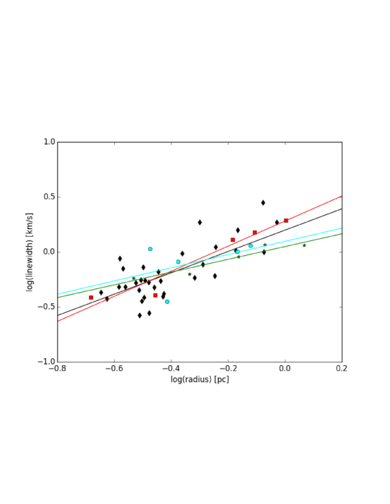
Figure 11: Size-linewidth relation of $\mathrm{{}^{13}CO}$ (2-1) brightness temperature clumps. The best fit line of all clumps is given by $\mathrm{\sigma=(1.58\pm 0.18)r^{(0.97\pm 0.12)}}$. The red squares are clumps in the red dendrogram structure in Figure  3 a ($\mathrm{\sigma=(1.91\pm 0.31)r^{(1.14\pm 0.19)}}$), the green stars are those that are in the green structure in Figure  3 a ($\mathrm{\sigma=(1.12\pm 0.11)r^{(0.58\pm 0.11)}}$), and the cyan circles are clumps in the cyan structure in Figure  3 a ($\mathrm{\sigma=(1.25\pm 0.69)r^{(0.60\pm 0.48)}}$). The red line is the best-fit line to the red squares, the green line is the best-fit line to the green stars, and the cyan line is the best-fit line to the cyan circles. There are a total of 5 each of red squares, green stars, and cyan circles plotted.

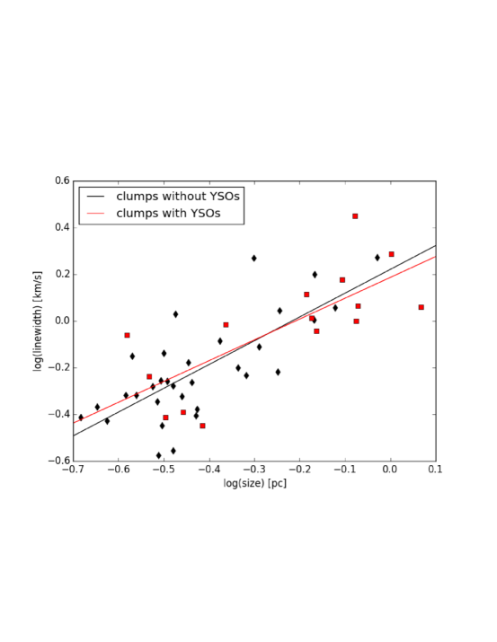
Figure 12: Size-linewidth relation of $\mathrm{{}^{13}CO}$ (2-1) column density clumps. The black diamonds are clumps not associated with any star formation and the best fit line is given by $\mathrm{\sigma=(1.66\pm 0.31)r^{(1.02\pm 0.17)}}$. The red squares show the clumps in our study that are are associated with star formation ($\mathrm{\sigma=(1.53\pm 0.25)r^{(0.89\pm 0.22)}}$). There is no noticeable difference in the slope or the intercept of the size-linewidth relation between clumps with active star formation and those without.

We investigate if the size-linewidth relation is dependent on the individual dendrogram structures. The size-linewidth relation of $\mathrm{{}^{13}CO}$ (2-1) column density clumps is $\mathrm{\sigma=(1.58\pm 0.18)r^{(0.97\pm 0.12)}}$ (Figure  11). The red squares are clumps in the red dendrogram structure in Figure  3 a ($\mathrm{\sigma=(1.91\pm 0.31)r^{(1.14\pm 0.19)}}$), the green stars are those that are in the green structure in Figure  3 a ($\mathrm{\sigma=(1.12\pm 0.11)r^{(0.58\pm 0.11)}}$), and the cyan circles are clumps in the cyan structure in Figure  3 a ($\mathrm{\sigma=(1.25\pm 0.69)r^{(0.60\pm 0.48)}}$). For each structure traced in different colors, we fit a slope and intercept. We compare the intercepts with each other and all the intercept values are 1-2$\mathrm{\sigma}$ away from each other. We then compare the slopes of the line fit to the different structures and we find the slopes are also 1-2$\mathrm{\sigma}$ away from each other. We then investigate if the size-linewidth is dependent upon if a clump is forming a star or not. The size-linewidth relation of $\mathrm{{}^{13}CO}$ (2-1) clumps that are associated with YSOs ($\mathrm{\sigma=(1.58\pm 0.18)r^{(0.90\pm 0.17)}}$) and those that are not ($\mathrm{\sigma=(1.86\pm 0.26)r^{(0.91\pm 0.14)}}$) in Figure  12. The size-linewidth of $\mathrm{{}^{13}CO}$ (2-1) clumps is the same for clumps with YSOs and those without. Individual star forming clumps have different mass, temperature, pressure conditions. Clumps with star formation taking place within them, and those with no observable star formation also should have different conditions. We thought local variations due to properties of the cloud or star formation happening would result in a different size-linewidth relation. However these differences in the local environment are negligible in comparison to the overall conditions in the regions of 30 Doradus we study in this work.

Larson’s first law suggests that the linewidth of a clump is only dependent on the size, $\mathrm{\sigma\propto r^{0.5}}$. We look into whether the universality of Larson’s first law applied to the clumps in 30 Doradus. We assume the clumps are self-gravitating and say the observed cloud mass is the virial mass:

$$M_{obs}=\frac{5\sigma^{2}r}{G}.$$ (1)

We can substitute the molecular gas surface density ($\mathrm{\Sigma=\frac{M_{obs}}{\pi r^{2}}}$) and solve for the linewidth:

$$\sigma=\left(\frac{\pi G}{5}\right)^{0.5}\Sigma^{0.5}r^{0.5}.$$ (2)

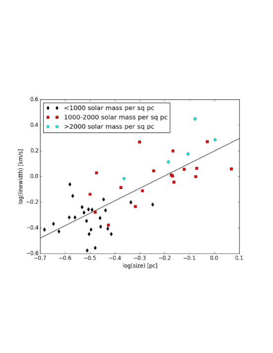
Figure 13: Size-linewidth relation of $\mathrm{{}^{13}CO}$ (2-1) column density clumps. The best fit line is $\mathrm{\sigma=(1.58\pm 0.18)r^{(0.97\pm 0.12)}}$. Black diamonds are clumps with mass density less than 1000 $\mathrm{M_{\odot}\;pc^{-2}}$, red squares are clumps with mass density between 1000-2000 $\mathrm{M_{\odot}\;pc^{-2}}$, and cyan circles are clumps with mass density above 2000 $\mathrm{M_{\odot}\;pc^{-2}}$.

The linewidth of a clump depends on the spatial extent as well as the mass surface density. Figure  13 shows the size-line width for $\mathrm{{}^{13}CO}$ (2-1) colorized by mass surface density: black diamonds for clumps with mass density less than 1000 $\mathrm{M_{\odot}\;pc^{-2}}$, red squares are clumps with mass density between 1000-2000 $\mathrm{M_{\odot}\;pc^{-2}}$, and cyan circles are clumps with mass density above 2000 $\mathrm{M_{\odot}\;pc^{-2}}$. We find clumps with larger sizes and linewidths tend to have larger mass surface densities.

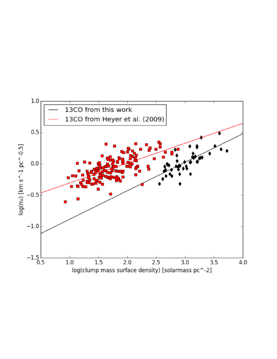
Figure 14: The dependence of $\mathrm{\frac{\sigma}{r^{0.5}}}$ on $\mathrm{\Sigma}$. The black line ($\mathrm{\nu=(0.04\pm 0.02)\Sigma^{(0.45\pm 0.06)}}$) is the best-fit line is going through $\mathrm{\nu}$ versus $\mathrm{\Sigma}$ of 30 Doradus clumps in this study. The red line ($\mathrm{\nu=(0.24\pm 0.02)\Sigma^{(0.31\pm 0.04)}}$) is the best-fit line going through $\mathrm{\nu}$ versus $\mathrm{\Sigma}$ of clumps studied by Heyer et al. (2009). The dependence on $\Sigma$ is contradictory to Larson’s scaling relation, but consistent with the slope found by Heyer et al. (2009).

We follow a similar approach to Heyer et al. (2009) and look at the dependence of the size and linewidth on the mass surface density. Heyer et al. (2009) find that Larson’s scaling relations are not universal. If $\mathrm{\Sigma}$ in Equation 2 is constant, then you can recover Larson’s first law ($\mathrm{\sigma=\nu\;r^{0.5}}$, where $\mathrm{\nu}$ is a constant). This means that $\mathrm{\frac{\sigma}{r^{0.5}}}$ = $(\mathrm{\frac{\pi G\Sigma}{5}})^{0.5}$ = $\mathrm{\nu}$, which is a constant. If Larson’s first law is to hold, then we should see a flat horizontal line when we plot $\mathrm{\nu}$ versus $\mathrm{\Sigma}$. Figure  14 shows that $\mathrm{\nu}$ is not constant with respect to $\mathrm{\Sigma}$, which is contradictory to Larson’s first scaling law. We find that $\mathrm{\nu\propto\Sigma^{0.45}}$. This is similar to the study done by Heyer et al. (2009). They too find a dependence of $\mathrm{\frac{\sigma}{r^{0.5}}}$ on $\mathrm{\Sigma}$ (Figure 7 in their paper). The slope of the line is not reported in their paper. We take the linewidth, size, and mass values they report and calculate $\mathrm{\nu}$ and $\mathrm{\Sigma}$. Heyer et al. (2009) results show that $\mathrm{\nu\propto\Sigma^{0.31}}$. Our findings of scaling relations between size, linewidth, and mass surface density lead us to the same conclusion as Heyer et al. (2009): Larson’s velocity scaling relationships are not universal.

5.2 Energy Balance

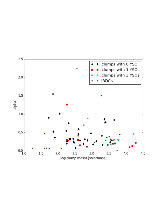
Figure 15: Figure showing the relation between the virial parameter versus the mass of the clump. We define $\alpha$ to equal to $\mathrm{\frac{5\sigma^{2}\;r}{G\;M}}$. Black diamonds are clumps with no YSO candidates, red squares are clumps with 1 YSO candidate, and cyan circles are clumps with 3 YSO candidates. Green stars are from infrared dark cloud studies by Gibson et al. (2009); Bontemps et al. (2010); Peretto et al. (2013).

We can further analyze the dynamics of the clumps by comparing the kinetic energy and the gravitational energy. We define the virial parameter, $\alpha$, to equal to $\mathrm{\frac{5\sigma^{2}\;r}{G\;M}}$ (Rosolowsky et al., 2008) (McKee & Zweibel, 1992) - the ratio of the kinetic potential energy to the gravitational potential energy. When $\alpha\textless 1$, the object is self-gravitating. Figure  15 shows the virial parameter as a function of clump mass on a log-log plot. The smaller mass clumps embedded within the larger mass clumps have a larger kinetic energy compare to the larger mass. We find larger clumps to have a larger gravitational potential energy than the smaller clumps: 72$\%$ of the $\mathrm{{}^{13}CO}$ (2-1) clumps have a virial parameter equal to 1 or less. Larger clumps in this study tend to have multiple YSO candidates, whereas smaller clumps tend to have one or no YSO candidates associated with them.

We compare our results with Milky Way studies in order to see how star-forming clumps in two different galaxies differ from each other. We plot virial parameter versus clump mass of infrared dark clouds studies by Gibson et al. (2009); Bontemps et al. (2010); Peretto et al. (2013) in Figure  15. These Milky Way clumps found via analysis of dark clouds could contain a few massive YSOs or hundreds of low-mass YSOs (Bontemps et al., 2010). Mass constraints on these stars have not been placed yet. ALMA observations of Dark cloud SDC335.579-0.272 show that it is one of the most massive, compact protostellar cores ever observed in the Galaxy and could potentially form an OB cluster similar to the Trapezium cluster in Orion (Peretto et al., 2013). The virial parameter versus mass value of this cluster is located close to the gravitationally bound massive star forming clumps in Figure  15 (the green star located at the bottom right). Orion is the nearest region of massive star formation, and therefore Orion and massive star formation sites similar to Orion provide the best comparison to 30 Doradus. Figure  15 shows star formation can take place in a wide range of conditions within infrared dark clouds: there are several low-mass gravitationally-unbound clumps that are forming stars and gravitationally-bound clumps 1000s of solar masses in size that are forming stars. However the virial conditions of dark cloud SDC335.579-0.272, a potential massive star formation location in the Milky Way, seems similar to massive star forming clumps in 30 Doradus.

There are a total of 15 star forming clumps, out of which 14 have a virial parameter equal to 1 or less. The majority (75$\%$) of clumps with masses greater than log(clump mass)=3.5 are associated with a YSO, but only 17$\%$ of clumps with masses less than log(clump mass)=3.5 are associated with a newly forming star. It is possible that the $\mathrm{{}^{13}CO}$ (2-1) line is not fully thermalized, therefore leading to an underestimate of the true mass. If the mass we report is underestimated, then the virial parameter we calculate would be overestimated. The points in Figure  15 would shift down and to the right in this hypothetical scenario if we could calculate the true mass. We would still find 14, or perhaps even all 15, of the star forming clumps to be gravitationally bound ($\alpha\textless 1$). We would also still find the majority of high-mass clumps are associated with star formation. We do not have the whole CO ladder to calculate the true mass, however the possibility of $\mathrm{{}^{13}CO}$ (2-1) not being fully thermalized does not affect our conclusions about the dynamical state of the clumps.

5.3 Which Clumps Have Newly Forming Stars and Which Do Not

We use the effective radius of the column density clumps to determine if there are any YSOs associated with the clumps. We find 7/87 more evolved low-mass YSOs and 7/10 massive young YSO candidates are associated with clumps. The 7 massive YSOs that are found within a clump are: [1] J84.703995-69.079110 , [2] J84.695932-69.083807, [4] J84.688990-69.084695, [5] J84.695173-69.084857, [7] J84.720292-69.077084, [8] J84.688372-69.078168, [9] J84.669113-69.081638 (the numbers are the same as those in Table 6). The reason for a higher percentage of massive YSOs to be associated with clumps than low-mass YSOs is consistent with massive YSOs being at an earlier evolutionary stage. The molecular cloud surrounding stars quickly dissipate due to the strong UV radiation from the central stars. Massive YSOs are much younger than low-mass YSOs in this study and therefore still can sometimes be found in their parental cloud. We are missing low-mass embedded YSOs. Tachihara et al. (2001) study the Lupus star-forming region with $\mathrm{{}^{12}CO}$ NANTEN data and find 40$\%$ of the more evolved low-mass YSOs in their study are associated with clumps less than $\textless 20\;\mathrm{M_{\odot}}$, which suggests that more evolved low-mass YSOs form in small clouds and then the parental cloud rapidly dissipates. We see more evolved low-mass YSOs (stars less than 3 $\mathrm{M_{\odot}}$ in Figure 17 a) projected against, and thus perhaps forming in clouds a few hundred solar masses to several tens of thousands solar masses. It is not clear if the lack of many more evolved low-mass YSOs associated with clumps is due to them moving away from the parental clump over time or if the parental clump of the young star has dissipated over time. Another reason of finding a smaller fraction of more evolved low-mass YSOs associated with clumps is because low-mass YSOs are fainter and harder to detect due to the sensitivity limits of the surveys.

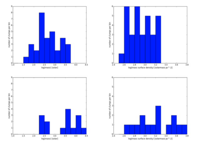
Figure 16: Left Column: Mass distribution of clumps without (top) and with (bottom) YSO candidates. Right Column: Mass surface density distribution of clumps without (top) and with (bottom) YSO candidates.

Figure  16 shows the difference in clump mass and $\mathrm{H_{2}}$ mass surface density distributions between clumps that do contain massive or low-mass YSOs versus clumps that do not. The distributions of clumps with massive or low-mass YSOs and those without are very different. The mass distribution of clumps without massive or low-mass YSOs is quasi normal, and the mass surface density distribution of clumps without massive or low-mass YSOs is uniform. Both the mass distribution and the mass surface density distribution of clumps with massive or low-mass YSOs are mostly uniform, but do have a noticeable peak in the center. The mass distribution and mass surface density distribution of clumps with star formation span a higher range in values than those without star formation: for example Figure  16 shows clumps without any stars have masses up to log(clump mass) = 3.75, but clumps with YSOs have masses up to log(clump mass) = 4.50. The average mass, column density, and mass surface density of clumps without any YSOs are 957 $\mathrm{M_{\odot}}$, $6.1\times 10^{22}\;\mathrm{cm^{-2}}$, and 957 $\mathrm{M_{\odot}\;pc^{-2}}$. The distribution of clumps with massive or low-mass YSOs is centered at x6 higher mass, x2 higher column density, and x2 higher mass surface density. Figure  17 a shows the mass of YSO versus the clump mass. Structures are designed such that the clumps may be concentric (one clump within another clump), therefore there are stars that are counted more than once. If a YSO is associated with a small clump, then it is also associated with the larger clump the smaller clump is embedded in. Only 20$\%$ of clumps smaller than 1778 $\mathrm{M_{\odot}}$ ($10^{3.25}\;\mathrm{M_{\odot}}$) have a YSO above 10 $\mathrm{M_{\odot}}$, whereas 66$\%$ of clumps larger than 1778 $\mathrm{M_{\odot}}$ have a YSO above 10 $\mathrm{M_{\odot}}$. Figure  17 b shows that 46$\%$ of clumps with $\mathrm{H_{2}}$ mass surface density less than 2512 $\mathrm{M_{\odot}\;pc^{-2}}$ ($10^{3.40}\;\mathrm{M_{\odot}\;pc^{-2}}$) have a massive YSO, but 71$\%$ of of clumps with mass surface density more than 2512 $\mathrm{M_{\odot}\;pc^{-2}}$ have a massive YSO. Larger mass clumps are more likely to form larger mass stars than smaller mass clumps.

The lowest surface density clump with a massive YSO forming in it provides us with a lower limit on the threshold above which high-mass star formation can occur: massive star formation appears to occur in clumps with mass $\textgreater 1.83\times 10^{2}\;\mathrm{M_{\odot}}$, surface density $\textgreater 6.67\times 10^{2}\;\mathrm{M_{\odot}\;pc^{-2}}$, and turbulence $\textgreater 1.18\;\mathrm{km/s}$. It is possible there are clumps with lower masses and lower surface densities forming low-mass YSOs. Future studies that find lower mass YSOs may push this mass surface density value lower. However, 30 Doradus is a very extreme star forming environment and more turbulent than typical GMCs in the Milky Way. The specific region we are analyzing in this study is 10 pc North of the R136 supercluster and is most likely influenced by the radiation field of R136. If there is more turbulence, then we would need higher densities and mass surface densities for star formation to occur. The mass surface density threshold in this study is 5 to 6 times higher than mass thresholds necessary to form stars as observed by Heiderman et al. (2010); Lada et al. (2010); Kennicutt & Evans (2012). Heiderman et al. (2010) use extinction maps to determine the gas surface density of Galactic star forming regions and find a threshold of 129 $\mathrm{M_{\odot}\;pc^{-2}}$. Lada et al. (2010) find similar values for the gas surface density: 116 $\mathrm{M_{\odot}\;pc^{-2}}$. The thresholds determined from Galactic studies applies to low-mass star formation. The surface density threshold of $\textgreater 6.67\times 10^{2}\;\mathrm{M_{\odot}\;pc^{-2}}$ we place in the ALMA footprint of 30 Doradus is for massive star formation.

Dunham et al. (2011) study high density gas tracer $\mathrm{NH_{3}}$ and measure an average mass density threshold of 176 $\mathrm{M_{\odot}\;pc^{-2}}$ for star forming clumps in the Milky Way. Rathborne et al. (2014) study nearby clouds and compare them to clouds in the CMZ. Observations of solar neighborhood clouds suggest a column density threshold of $1.4\times 10^{22}\;\mathrm{cm^{-2}}$ (Lada et al., 2010). However the universality of this value is questioned since theoretical models predict the threshold for star formation is dependent on the density and the Mach number (Krumholz & McKee, 2005). Even though the CMZ has a much higher column density than $1.4\times 10^{22}\;\mathrm{cm^{-2}}$, it is producing orders of magnitude less stars than predicted. Rathborne et al. (2014) find that the density threshold for star formation locally is $10^{4}\;\mathrm{cm^{-3}}$, however the CMZ with much higher turbulence has a density threshold of $10^{8}\;\mathrm{cm^{-3}}$. Star formation is dependent on the local environment, with regions of high turbulence having a higher threshold to overcome in order for the star formation process to occur.

6 Conclusion

We look at YSOs that are within the ALMA CO footprint of 30 Doradus to conduct a comprehensive analysis of the molecular gas and the stars that form within them. We analyze the CO clumps using dendrograms. The $\mathrm{{}^{13}CO}$ (2-1) molecular gas clumps analyzed using dendrograms have sizes that range from 0.23 - 1.17 pc, masses that range from 53 - 19300 $\mathrm{M_{\odot}}$, and linewidths that range from 0.27 - 2.81 km/s. There are several conclusions we come to with our analysis of CO clumps and YSOs as listed below.

1. We find $\mathrm{{}^{13}CO}$ (2-1) clumps to have a larger linewidth for a given size than previous studies done with the Perseus cloud (Shetty et al., 2012). A larger linewidth is not dependent on the size scale, and not dependent on if star formation is taking place in a clump or not. Local environmental factors (high star formation rate, high densities, and high pressures) in 30 Doradus can explain why we find clumps to have a larger linewidth for a given size. Our result is similar to studies by Shetty et al. (2012) who find clumps in the CMZ have a slope of 0.5 in the size-linewidth relation, but are offset higher compared to the Perseus cloud due to the local environmental conditions. We find the slope of the size-linewidth relation of $\mathrm{{}^{12}CO}$ (2-1) and $\mathrm{{}^{13}CO}$ (2-1) molecular gas to be consistent within 3$\mathrm{\sigma}$ of previous studies (Bolatto et al., 2008; Heyer et al., 2009; Shetty et al., 2012).

2. Higher mass clumps have a tendency to have a lower viral parameter and contain multiple YSOs in comparison to lower mass clumps.

3. We find a total of 10 massive YSOs (4 new YSO candidates) with masses between 8.5-24.0 $\mathrm{M_{\odot}}$, and 87 more evolved low-mass YSOs with masses between 1-3 $\mathrm{M_{\odot}}$ in the region of interest.

4. There is a difference in distribution of the mass and $\mathrm{H_{2}}$ column density of clumps that do not contain any newly forming stars and those that do. The mass and column density of clumps without stars falls off quickly and tend to be lower on average than clumps with stars. The clumps that has the lowest surface density, but still hosts a massive YSO candidate provides us with lower limits necessary for star formation. It is necessary for clumps to have high masses ($\textgreater 1.83\times 10^{2}\;\mathrm{M_{\odot}}$), high linewidths (v $\textgreater 1.18\;\mathrm{km/s}$), and high mass densities ($\textgreater 6.67\times 10^{2}\;\mathrm{M_{\odot}\;pc^{-2}}$) in order for massive star formation to occur. This threshold was found by looking at the least massive $\mathrm{{}^{13}CO}$ clump that is forming a massive YSO.

5. A higher fraction of young and massive YSO candidates are found within clumps (7/10) than the more evolved low-mass YSOs (7/87). This is because the more evolved low-mass YSOs in this study are older, and therefore have moved away from their parental clump. Our inventory of young forming stars is not sensitive to the very embedded low-mass YSOs.

6. We look at the dependence of the size-linewidth relation to the mass surface density. There is a dependence of $\mathrm{\frac{\sigma}{r^{0.5}}}$ on $\mathrm{\Sigma}$. This is contradictory to Larson’s scaling relationships. Assuming the clumps are is gravitational equilibrium and making relevant substitutions (see Section 5.1), we derive $\sigma=\left(\frac{\pi G}{5}\right)^{0.5}\Sigma^{0.5}r^{0.5}$. Larson’s third scaling relation states that $\Sigma$ is approximately constant for all clouds. Re-arranging the equation we derived and taking into account Larson’s third scaling relations leads to the conclusion that the slope of $\mathrm{\frac{\sigma}{r^{0.5}}}$ versus $\mathrm{\Sigma}$ should be 0. However we do not find the slope to be 0 (Figure 14). It is possible that Larson’s scaling relationships are not universal.

7. The virial parameter of massive clumps in 30 Doradus forming multiple YSOs is similar to SDC335.579-0.272, an infrared dark cloud in the Milky Way that is most likely forming massive stars.

Appendix

Appendix A Calculating $\mathrm{H_{2}}$ mass using $\mathrm{N_{13CO}}$

We assume that $\mathrm{{}^{13}CO}$ is optically thin. The optical depth of $\mathrm{{}^{13}CO}$ is given by:

$$\mathrm{\tau_{{}^{13}CO(2-1)}}=\mathrm{-ln[1-\frac{T_{B,^{13}CO(2-1)}}{10.6}([e^{10.6/T_{ex,^{12}CO(2-1)}}-1]^{-1}-0.02)^{-1}]},$$ (A1)

where the excitation temperature is given by:

$$\mathrm{T_{ex,^{12}CO(2-1)}}=\mathrm{\frac{10.6\;K}{ln(1+\frac{10.6\;K}{T_{B,^{12}CO(2-1)}+0.21\;K})}}.$$ (A2)

The $\mathrm{{}^{12}CO}$ excitation temperature is only dependent on the $\mathrm{{}^{12}CO}$ brightness temperature because we assume $\mathrm{{}^{12}CO}$ to be optically thick. The $\mathrm{{}^{12}CO}$ is likely to be optically thick if $\mathrm{{}^{13}CO}$ is present because a larger column of molecular has is needed to see $\mathrm{{}^{13}CO}$, as oppose to $\mathrm{{}^{12}CO}$. The $\mathrm{{}^{13}CO}$ map is the mask and we do not impose an artificial mask on the excitation temperature. There are places where the optical depth (equation A1) does not make sense, and therefore gives a column density value that is not believable, which has been masked out. For example, there are pixels for which the optical depth is negative or infinity because of the natural log and an exponent of -1 in equation A1. This is because of how you clean the ALMA data. These pixels with negative values of values that equal infinity are not real or believable, but rather an artifact of the data cube quality. Further assumptions of the local thermodynamic equilibrium (or LTE) analysis include: $\mathrm{{}^{13}CO}$ has the same excitation temperature as $\mathrm{{}^{12}CO}$, CO is thermalized (level population is described by the Boltzmann equation), and the abundance ratio between $\mathrm{{}^{12}CO}$ and $\mathrm{{}^{13}CO}$ is constant. The total $\mathrm{{}^{13}CO}$ column density is then given by the equation:

$$\mathrm{N_{{}^{13}CO,tot}}=\mathrm{\frac{1.5\times 10^{14}\;T_{ex}\;e^{5.3/T_{ex}}\;\int\tau dv}{1-e^{-10.6/T_{ex}}}}.$$ (A3)

We assume $\mathrm{\frac{H_{2}}{{}^{13}CO}}=5\times 10^{2}$ (Indebetouw et al., 2013) to convert the $\mathrm{{}^{13}CO}$ column density to $\mathrm{H_{2}}$ column density. The total $\mathrm{H_{2}}$ mass is then derived by:

$$\mathrm{M}=\mathrm{m_{H_{2}}\;\int N_{H_{2}}dA}.$$ (A4)

Appendix B Comparison Between Cprops and Astrodendro

Due to the different algorithm used by Indebetouw et al. (2013) (cprops), it is not possible to have a 1:1 relation between the clumps identified in this work and those published by Indebetouw and collaborators. Therefore we pick three clumps we identify by eye that are similar in the output of both programs to compare to each other. We compare the clump properties listed in Table 2 in this work, to the clump properties from Indebetouw et al. (2013). We used the same definition of sizes and linewidths when comparing clump properties by Indebetouw et al. (2013) and the results from this work. We got the size and linewidth values of $\mathrm{{}^{13}CO}$ clumps output from cprops from our personal correspondence with Remy Indebetouw. Definition of sizes and linewidths is further described in Appendix C. The two algorithms (cprops and astrodendro) work in different ways and therefore not possible to select a clump output from one program, and match it to the same exact clump output from the other program. And we cannot do this for all the leaves and branches output from the dendrogram program. We match the $\mathrm{{}^{13}CO}$ clumps output from cprops to the same clumps identified by astrodendro, i.e. we search for clumps output from the two different algorithms and find those that are within 1 clump radii of each other. There are a total of 8 such clumps we can match from the two different algorithms and their properties are listed below. The purpose of this comparison is to see if we can find clump mass and size properties output from the two programs that are not different by orders of magnitude.

For the first clump listed in the table below we find that the astrodendro picks out a size that is twice as high as the size calculated from cprops, however the linewidth calculated by astrodendro is about 70$\%$ of the linewidth calculated by cprops. The next four clumps listed in the table below are comparable in size output from cprops and astrodendro, however the linewidths calculated by astrodendro are lower by 60-80$\%$. Clumps selected by astrodendro that are larger or comparable in size to clumps selected by cprops tend to have lower linewidths. The next two in the table below are $\mathrm{{}^{13}CO}$ clumps selected by astrodendro that are smaller in size than the same clumps selected by cprops. The size derived by astrodendro for the two clumps is smaller by a fact of 60-70$\%$, however the linewidths are smaller by a factor of 40-50$\%$. Astrodendro systematically calculates smaller linewidths, which explains the offset of the Indebetouw et al. (2013) clumps from the clumps we derived in this paper. If we assume the clumps selected with astrodendro have lower linewidths than the clumps selected with cprops by a factor of 60-80$\%$ (as in the case for comparable size clumps), we can calculate this shift in the cprops clumps shown in cyan in Figure 10. The equation of the best fit line going through the cprops clumps in Figure 10 is given by $\mathrm{\sigma=(2.39\pm 0.33)r^{(0.91\pm 0.15)}}$. Shifting this line down by 60-80$\%$ changes the intercept of 2.39 to be between 1.69 to 1.99. The equation of the best fit line going through the astrodendro clumps in Figure 10 is given by $\mathrm{\sigma=(1.58\pm 0.18)r^{(0.97\pm 0.12)}}$. After taking into account the offset to lower linewidths inherent to astrodendro, the best fit-line going through the $\mathrm{{}^{13}CO}$ cprops clumps and the best-fit line going through the $\mathrm{{}^{13}CO}$ astrodendro clumps are in agreement within 1$\sigma$.

Table B.1: Comparing Cprops and Astrodendro Outputs

Size [$\mathrm{pc}$]	$\sigma$ [$\mathrm{km/s}$]	$\mathrm{{}^{12}CO}$	$\mathrm{{}^{12}CO}$	$\mathrm{{}^{12}CO}$	Mass Derived	$\mathrm{{}^{13}CO}$	$\mathrm{{}^{13}CO}$	$\mathrm{{}^{13}CO}$	Mass Derived
From Cprops	From Cprops	ID	Size [$\mathrm{pc}$]	$\sigma$ [$\mathrm{km/s}$]	From $\mathrm{{}^{12}CO}$ [$\mathrm{M_{\odot}}$]	ID	Size [$\mathrm{pc}$]	$\sigma$ [$\mathrm{km/s}$]	From $\mathrm{{}^{13}CO}$ [$\mathrm{M_{\odot}}$]
0.35	0.57	26	0.34	0.68	259	0	0.73	0.39	297
0.28	0.87	53	0.17	0.94	62	16	0.32	0.55	112
0.32	0.94	69	0.32	0.95	359	22	0.32	0.73	612
0.36	0.78	28	0.31	0.84	271	4	0.35	0.48	281
0.48	1.15	94	0.31	0.98	851	41	0.42	0.82	2050
0.44	1.37	67	0.20	0.65	206	15	0.29	0.58	385
0.39	0.96	80	0.41	1.0	681	27	0.28	0.48	232
0.51	1.36	98	0.19	0.47	125	39	0.34	1.07	934

Note. — Column 1: Clump size derived from cprops. Column 2: The linewidth derived from cprops. Column 3: $\mathrm{{}^{12}CO}$ clump ID as listed in Table 3. Column 4: $\mathrm{{}^{12}CO}$ clump radius as listed in Table 3. Column 5: The linewidth of $\mathrm{{}^{12}CO}$ clumps in this study. Column 6: $\mathrm{H_{2}}$ mass derived using $\mathrm{{}^{12}CO}$. Column 7: $\mathrm{{}^{13}CO}$ clump ID as listed in Table 4. Column 8: $\mathrm{{}^{13}CO}$ clump radius. Column 9: The linewidth of $\mathrm{{}^{13}CO}$ clumps in this study. Column 10: $\mathrm{H_{2}}$ mass derived using $\mathrm{{}^{13}CO}$.

Appendix C Defining Sizes and Linewidths

There are many definitions of clump ‘sizes’ and many ways to calculate a ‘linewidth’ of a data cube. These definitions vary significantly in the literature. In Indebetouw et al. (2013), the size was measured by fitting a 2-dimensional ellipse to the half-power contour of each clump. The ellipse was then deconvolved in two dimensions with the beamsize, and the radius quoted in Indebetouw et al. (2013) was 1.91 times the geometric mean of that deconvolved ellipse semimajor and semiminor axes. At time of writing Indebetouw et al. (2013), the ellipse-fitting measure of size was compared to spatial moments and to fitting a two dimensional Gaussian to the spatial distribution of emission, and found to be in agreement within error, but the most robust of the three methods. In this paper, for both the Indebetouw et al. (2013) clumps and those defined by astrodendro, the size is calculated from the weighted second moment in two spatial directions, specifically the direction of greatest spatial extent and perpendicular to that. The radius is then 1.91 times the geometric mean of those two spatial second moments. In particular it should be noted that the current numbers thus include convolution by the $\sim$ 0.5pc beam.

In Indebetouw et al. (2013), the linewidth was calculated for each clump by extracting the ‘column’ through the cube, i.e. for each pixel in the clump, the pixels covering the full velocity range of the cube. A Gaussian was then fitted to the spectrum of that ‘column’, and the width, deconvolved by the spectral resolution of 0.35km/s, was reported. The fitted spectrum thus includes velocity line wings which are not explicitly assigned to the clump by the decomposition. At the time of writing Indebetouw et al. (2013), each spectrum was carefully examined, and verified that effects such as two clumps along the same line of sight artificially broadening the linewidth did not occur. That Gaussian fitting linewidth calculation was compared to the weighted second moments in velocity of only the clump-assigned pixels, and of the entire ‘column’ through the cube. Results were within uncertainties, but fitting a Gaussian to the ‘column’ was more robust. For the current comparison, we use the weighted velocity second moment of the pixels assigned to the cprops clump or astrodendro structure. The Indebetouw et al. (2013) method could over-estimate the linewidth, if significant emission is along the line of sight, whereas the current method likely underestimates the linewidth of a structure, since PPV and PPP space do not precisely correspond. As with the sizes, the current reported linewidths include the effects of finite spectral resolution, but that is less than a 2% effect for the linewidths under consideration. The slight difference between the cprops and astrodendro 30 Doradus clumps seen in Figure  10 can be attributed to the difference between the two algorithms, how they pick out the structure, and the input thresholds used.

Figure 1: Top: HST F160W in greyscale, ALMA+APEX $\mathrm{{}^{12}CO}$ (2-1) in contour (contour levels signify 10$\%$, 20$\%$, 30$\%$, 40$\%$, 60$\%$, and 80$\%$ of peak integrated flux), and the location of more evolved low-mass YSOs (as discussed in section 4.1) in green circles . North is to the upper-left in this figure. Bottom: HST F160W in greyscale, ALMA+APEX $\mathrm{{}^{12}CO}$ (2-1) in contour (contour levels signify 10$\%$, 20$\%$, 30$\%$, 40$\%$, 60$\%$, and 80$\%$ of peak integrated flux), and the location of all point sources in the SAGE catalog in green circles. Numbers 1-10 are massive YSO candidates (as discussed in section 4.2), and number 11-15 are SAGE point sources in the footprint we do not consider to be YSOs. The number near the YSO candidates indicates rank in mass (1 is the most massive YSO candidate and 10 in the least massive YSO candidate).

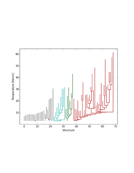
Figure 2 a: Dendrogram hierarchy of $\mathrm{{}^{12}CO}$ (2-1) brightness temperature. The trunks represent the lowest lever of emission. The trunks are connected to leaves, which represent higher emission clumps.

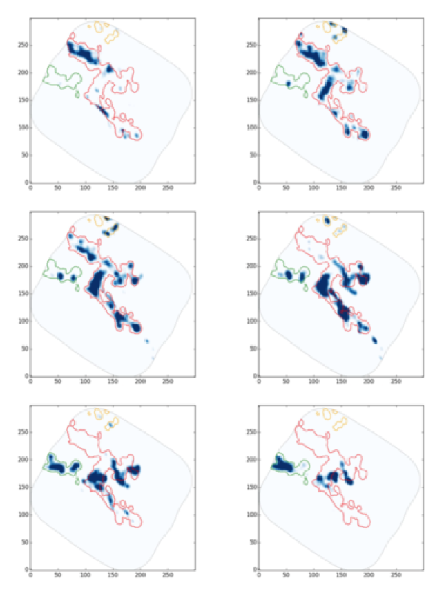
Figure 2 b: Slices of the $\mathrm{{}^{12}CO}$ (2-1) brightness temperature velocity cube is shown in blue color. From left-to-right, top-to-bottom the channel velocities are 245.17 km/s, 247.17 km/s, 249.17 km/s, 251.17 km/s, 253.17 km/s, and 255.17 km/s. The red, green, and orange molecular structures highlighted correspond to the red, green, and cyan dendrogram structure in Figure  2 a.

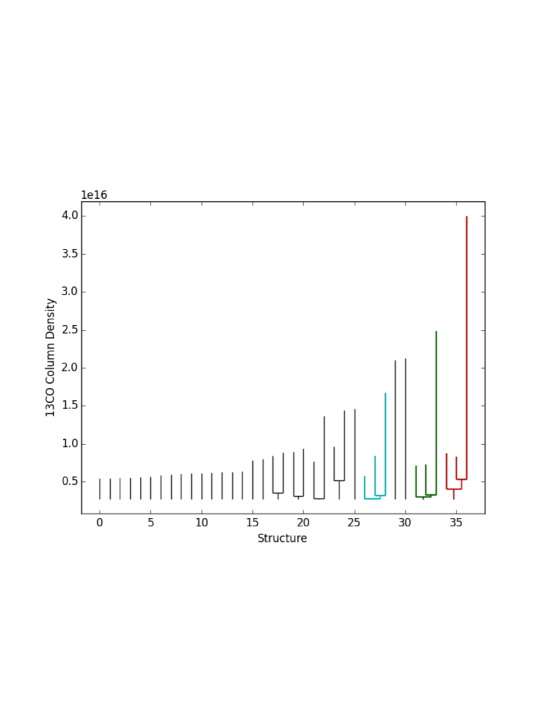
Figure 3 a: Dendrogram hierarchy of $\mathrm{{}^{13}CO}$ (2-1) column density.

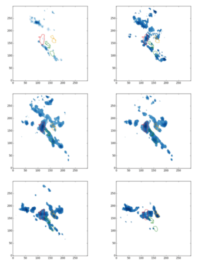
Figure 3 b: Slices of the $\mathrm{{}^{13}CO}$ (2-1) column density velocity cube is shown in blue color. From left-to-right, top-to-bottom the channel velocities are 245.17 km/s, 247.17 km/s, 249.17 km/s, 251.17 km/s, 253.17 km/s, and 255.17 km/s. The red, green, and orange molecular structures highlighted correspond to the red, green, and cyan dendrogram structure in Figure  3 a.

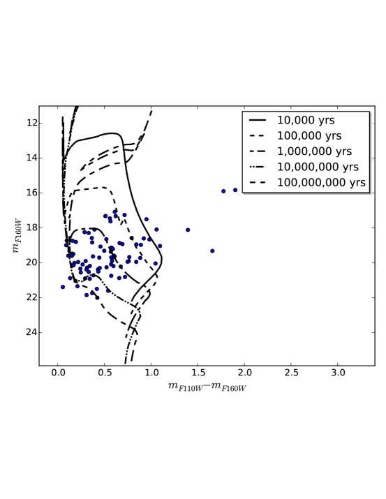
Figure 4 a: F160W versus F110W - F160W CMD with isochrones. The isochrones are from the Padova code (Bressan et al., 2012; Chen et al., 2015). The points are more evolved low-mass YSOs that have been selected via H$\mathrm{\alpha}$ excess and have been de-reddened (De Marchi et al., 2016), as discussed in section 4.1.

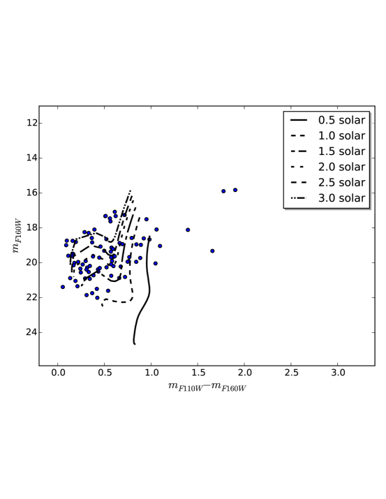
Figure 4 b: This is the same as Figure  4 a, however we plot F160W versus F110W - F160W CMD.

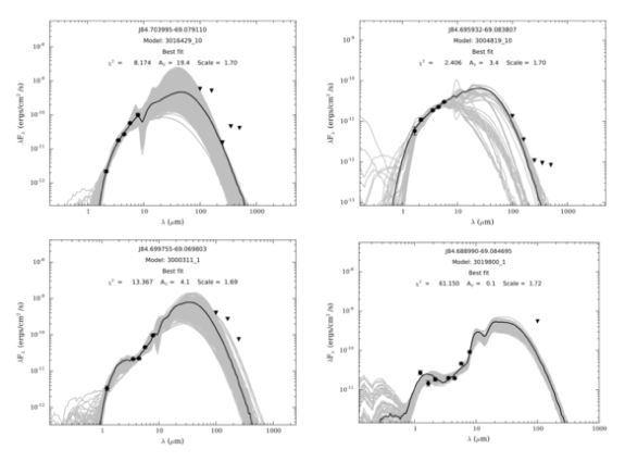
Figure 5: SED fits of all point sources in the SAGE catalog that are in the ALMA footprint of this study and are YSO candidates. They are ordered from top to bottom, left to right in order of highest mass to lowest mass. Black dots are the fitted data points, black triangles are upper limits, the black line is the best fit model, and the grey lines are all models that have $\mathrm{\chi^{2}}\textless 3$ relative to the best fit model.

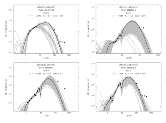
Figure 5 continued: SED fits of all point sources in the SAGE catalog that are in the ALMA footprint of this study and are YSO candidates. They are ordered from top to bottom, left to right in order of highest mass to lowest mass. Black dots are the fitted data points, black triangles are upper limits, the black line is the best fit model, and the grey lines are all models that have $\mathrm{\chi^{2}}\textless 3$ relative to the best fit model.

Figure 5 continued: SED fits of all point sources in the SAGE catalog that are in the ALMA footprint of this study and are YSO candidates. They are ordered from top to bottom, left to right in order of highest mass to lowest mass. Black dots are the fitted data points, black triangles are upper limits, the black line is the best fit model, and the grey lines are all models that have $\mathrm{\chi^{2}}\textless 3$ relative to the best fit model.

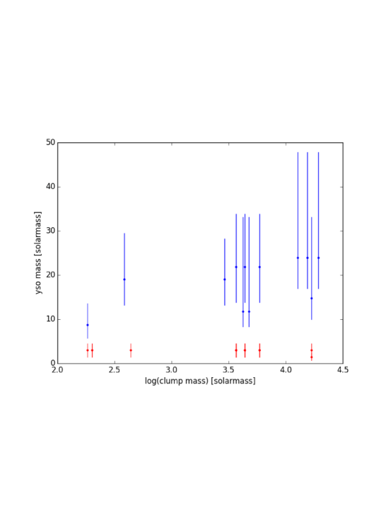
Figure 17 a: Star mass versus clump mass for each newly forming star. Red circles represent the low-mass more evolved YSO candidates selected via H$\mathrm{\alpha}$ excess. Blue circles represent the massive YSO candidates selected by SED fitting.

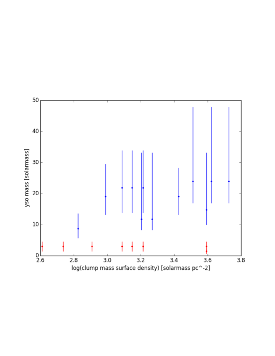
Figure 17 b: Star mass versus clump mass surface density for each newly forming star. Red circles represent the low-mass more evolved YSO candidates selected via H$\mathrm{\alpha}$ excess. Blue circles represent the massive YSO candidates selected by SED fitting.

Table 1: Mass Derived from $\mathrm{{}^{12}CO}$ (2-1)

Clump ID	RA	Dec	Radius [$\mathrm{pc}$]	$\mathrm{F_{{}^{12}CO}}$ [$\mathrm{K\;km\;s^{-1}}$]	Total Mass [$\mathrm{M_{\odot}}$]	Linewidth [km/s]
0	84.706989	-69.068853	0.522	21.2 $\pm$ 2.55	321 $\pm$ 38.6	1.29
1	84.700807	-69.078029	4.61	137 $\pm$ 17.5	98900 $\pm$ 12600	3.86
2	84.700775	-69.078057	4.59	139 $\pm$ 17.2	97300 $\pm$ 12100	3.83
3	84.700755	-69.078118	4.57	143 $\pm$ 16.7	93700 $\pm$ 10900	3.74
4	84.703518	-69.069242	0.457	23.2 $\pm$ 2.23	271 $\pm$ 26.1	2.18
5	84.700788	-69.078107	4.57	144 $\pm$ 16.4	90800 $\pm$ 10300	3.69
6	84.703853	-69.071507	0.454	47.2 $\pm$ 2.42	647 $\pm$ 33.2	2.44
7	84.700814	-69.078139	4.55	148 $\pm$ 15.5	83100 $\pm$ 8710	3.58
8	84.700823	-69.078138	4.55	148 $\pm$ 15.5	83400 $\pm$ 8740	3.59
9	84.698556	-69.079379	4.03	151 $\pm$ 13.5	63900 $\pm$ 5750	3.35
10	84.698567	-69.079381	4.02	151 $\pm$ 13.2	61700 $\pm$ 5390	3.3
11	84.698536	-69.079390	4.01	152 $\pm$ 12.8	58300 $\pm$ 4910	3.24
12	84.694103	-69.077254	2.25	148 $\pm$ 7.42	19100 $\pm$ 958	3.87
13	84.699955	-69.072633	0.287	27 $\pm$ 1.47	137 $\pm$ 7.45	1.04
14	84.699347	-69.075175	0.497	158 $\pm$ 2.40	2130 $\pm$ 32.4	3.41
15	84.696479	-69.077376	1.28	153 $\pm$ 5.07	9170 $\pm$ 304	4.43
16	84.707331	-69.071393	0.298	46.8 $\pm$ 1.54	261 $\pm$ 8.59	1.62
17	84.699810	-69.069712	1.54	53.6 $\pm$ 6.60	5440 $\pm$ 669	2.81
18	84.698967	-69.069816	1.36	61.7 $\pm$ 5.43	4240 $\pm$ 373	2.65
19	84.697151	-69.069254	0.257	35.5 $\pm$ 1.31	141 $\pm$ 5.21	1.17
20	84.693634	-69.080124	0.337	20.2 $\pm$ 1.71	138 $\pm$ 11.7	0.991
21	84.697258	-69.079987	0.273	13.7 $\pm$ 1.38	60.7 $\pm$ 6.11	0.535
22	84.710057	-69.073121	1.38	144 $\pm$ 6.82	15600 $\pm$ 738	2.18
23	84.695760	-69.082149	0.471	35.4 $\pm$ 2.23	411 $\pm$ 25.9	1.07
24	84.696537	-69.081386	0.243	21.7 $\pm$ 1.19	71.1 $\pm$ 3.89	0.511
25	84.689353	-69.081503	0.872	30.1 $\pm$ 3.26	749 $\pm$ 81.1	0.908
26	84.689385	-69.082348	0.338	34.7 $\pm$ 1.79	259 $\pm$ 13.4	0.683
27	84.700869	-69.080518	2.68	156 $\pm$ 10.0	36600 $\pm$ 2350	2.76
28	84.695538	-69.082384	0.311	45.4 $\pm$ 1.60	271 $\pm$ 9.55	0.84
29	84.702396	-69.079943	2.26	161 $\pm$ 9.11	31000 $\pm$ 1770	2.73
30	84.689291	-69.080981	0.526	29.7 $\pm$ 2.39	396 $\pm$ 31.9	0.803
31	84.688452	-69.081129	0.337	32.9 $\pm$ 1.76	237 $\pm$ 12.7	0.712
32	84.709587	-69.073393	0.864	159 $\pm$ 3.63	4900 $\pm$ 112	1.76
33	84.700921	-69.080487	2.66	159 $\pm$ 9.71	35100 $\pm$ 2140	2.70
34	84.702480	-69.079910	2.24	159 $\pm$ 9.00	30100 $\pm$ 1710	2.71
35	84.701184	-69.082238	0.715	71.3 $\pm$ 2.93	1440 $\pm$ 59.2	1.47
36	84.700356	-69.082942	0.372	62.3 $\pm$ 1.75	446 $\pm$ 12.5	0.541
37	84.702569	-69.079872	2.20	162 $\pm$ 8.61	27900 $\pm$ 1480	2.64
38	84.695010	-69.075487	0.358	24.8 $\pm$ 1.58	144 $\pm$ 9.17	1.70
39	84.700337	-69.069687	1.72	47 $\pm$ 7.23	5730 $\pm$ 881	2.75
40	84.691066	-69.080654	0.261	26.3 $\pm$ 1.30	103 $\pm$ 5.09	0.63
41	84.699043	-69.069825	1.33	66.3 $\pm$ 4.67	3370 $\pm$ 237	1.77
42	84.701829	-69.081685	0.381	68 $\pm$ 1.78	502 $\pm$ 13.1	0.903
43	84.708896	-69.079471	0.229	26.1 $\pm$ 1.13	77.4 $\pm$ 3.35	0.606
44	84.719623	-69.076736	1.73	146 $\pm$ 8.61	25300 $\pm$ 1490	3.54
45	84.715952	-69.071826	0.38	58.4 $\pm$ 1.56	332 $\pm$ 8.67	0.829
46	84.699158	-69.069782	1.32	65.3 $\pm$ 4.22	2710 $\pm$ 175	1.50
47	84.692969	-69.085462	0.202	29.9 $\pm$ 0.97	66.1 $\pm$ 2.14	0.451
48	84.688529	-69.085050	0.621	148 $\pm$ 3.26	3670 $\pm$ 80.9	1.59
49	84.693965	-69.084531	0.181	33.2 $\pm$ 0.84	54.4 $\pm$ 1.38	0.361
50	84.702648	-69.079743	2.18	174 $\pm$ 8.08	26400 $\pm$ 1230	2.28
51	84.719989	-69.076724	1.62	174 $\pm$ 7.41	22300 $\pm$ 949	3.41
52	84.720925	-69.076775	1.31	201 $\pm$ 6.44	19300 $\pm$ 621	3.30
53	84.693749	-69.082392	0.171	36.5 $\pm$ 0.85	62.1 $\pm$ 1.45	0.941
54	84.702724	-69.079712	2.16	175 $\pm$ 7.79	24700 $\pm$ 1090	2.21
55	84.704743	-69.078626	1.22	211 $\pm$ 5.87	16900 $\pm$ 471	2.34
56	84.721886	-69.076712	1.08	225 $\pm$ 5.57	16300 $\pm$ 404	3.17
57	84.715112	-69.070094	0.295	36.3 $\pm$ 1.53	201 $\pm$ 8.47	0.973
58	84.699190	-69.069651	1.34	63 $\pm$ 3.74	2040 $\pm$ 121	1.06
59	84.699174	-69.069684	1.35	60.6 $\pm$ 3.92	2170 $\pm$ 141	1.06
60	84.698488	-69.069178	0.919	70.0 $\pm$ 2.7	1190 $\pm$ 45.9	1.10
61	84.696900	-69.082925	1.02	115 $\pm$ 4.56	5590 $\pm$ 222	1.36
62	84.704867	-69.078592	1.15	221 $\pm$ 5.39	15100 $\pm$ 368	2.31
63	84.695507	-69.078140	0.954	151 $\pm$ 4.33	6540 $\pm$ 189	2.07
64	84.721953	-69.076703	0.987	242 $\pm$ 4.84	13300 $\pm$ 266	2.95
65	84.710659	-69.069206	0.731	13.3 $\pm$ 2.98	277 $\pm$ 62.1	1.08
66	84.696763	-69.069577	0.423	64.1 $\pm$ 1.85	511 $\pm$ 14.7	1.03
67	84.695439	-69.084713	0.202	90.3 $\pm$ 0.990	206 $\pm$ 2.26	0.645
68	84.705060	-69.078616	0.95	203 $\pm$ 4.18	83100 $\pm$ 1710	2.01
69	84.700879	-69.068490	0.321	71.6 $\pm$ 1.46	359 $\pm$ 7.32	0.949
70	84.705644	-69.078739	0.634	235 $\pm$ 3.07	5170 $\pm$ 67.5	1.34
71	84.695601	-69.078200	0.798	147 $\pm$ 3.60	4440 $\pm$ 109	1.94
72	84.695392	-69.078432	0.688	150 $\pm$ 3.08	3310 $\pm$ 67.9	1.87
73	84.700724	-69.070683	0.419	48.6 $\pm$ 2.05	477 $\pm$ 20.1	0.769
74	84.721433	-69.076804	0.704	248 $\pm$ 3.45	6870 $\pm$ 95.6	2.45
75	84.688778	-69.077411	0.932	131 $\pm$ 4.09	5110 $\pm$ 159	1.24
76	84.690076	-69.075857	0.328	83.4 $\pm$ 1.59	490 $\pm$ 9.34	1.11
77	84.697577	-69.070949	0.179	17.5 $\pm$ 0.820	27.7 $\pm$ 1.29	0.263
78	84.704109	-69.068918	0.501	37.7 $\pm$ 2.73	657 $\pm$ 47.6	1.13
79	84.681270	-69.089642	0.273	36.3 $\pm$ 1.39	163 $\pm$ 6.24	1.18
80	84.683899	-69.087016	0.414	54.4 $\pm$ 2.32	681 $\pm$ 29.1	1.00
81	84.696870	-69.082978	0.758	109 $\pm$ 3.34	2810 $\pm$ 86.1	0.993
82	84.688625	-69.077588	0.751	142 $\pm$ 3.70	4530 $\pm$ 118	1.21
83	84.714477	-69.077183	0.61	103 $\pm$ 3.10	2310 $\pm$ 69.5	1.66
84	84.681043	-69.088247	0.272	25.6 $\pm$ 1.41	118 $\pm$ 6.49	0.951
85	84.692264	-69.083296	0.211	33.6 $\pm$ 0.990	76.6 $\pm$ 2.26	0.413
86	84.701799	-69.079815	0.332	68.9 $\pm$ 1.54	384 $\pm$ 8.58	0.571
87	84.692210	-69.079778	0.184	52.7 $\pm$ 0.840	86.7 $\pm$ 1.38	0.495
88	84.698923	-69.070512	0.253	39.4 $\pm$ 1.24	142 $\pm$ 4.47	0.614
89	84.696715	-69.069817	0.209	19.9 $\pm$ 1.04	50.3 $\pm$ 2.63	0.357
90	84.692520	-69.083699	0.278	35.7 $\pm$ 1.36	154 $\pm$ 5.87	0.529
91	84.697617	-69.076296	0.218	78.5 $\pm$ 1.03	194 $\pm$ 2.54	0.814
92	84.703864	-69.079984	0.162	66.4 $\pm$ 0.750	88.1 $\pm$ 0.995	0.494
93	84.711315	-69.080377	0.322	9.25 $\pm$ 1.57	53.1 $\pm$ 9.01	0.403
94	84.694719	-69.079030	0.306	166 $\pm$ 1.48	851 $\pm$ 7.59	0.976
95	84.710370	-69.079071	0.311	36.2 $\pm$ 1.54	201 $\pm$ 8.55	0.492
96	84.702161	-69.078375	0.455	85.9 $\pm$ 1.99	793 $\pm$ 18.4	0.842
97	84.703010	-69.078498	0.251	82.0 $\pm$ 1.19	271 $\pm$ 3.93	0.422
98	84.696271	-69.077918	0.194	68.2 $\pm$ 0.890	125 $\pm$ 1.63	0.469
99	84.724458	-69.075500	0.165	40.9 $\pm$ 0.770	56.9 $\pm$ 1.07	0.361
100	84.701233	-69.078210	0.284	63.6 $\pm$ 1.25	233 $\pm$ 4.58	0.383
101	84.727933	-69.079484	0.738	11.7 $\pm$ 2.72	203 $\pm$ 47.2	0.934
102	84.728497	-69.079548	0.842	11.9 $\pm$ 2.98	249 $\pm$ 62.4	1.00
103	84.712801	-69.078013	0.273	31.5 $\pm$ 1.40	143 $\pm$ 6.34	0.965
104	84.709897	-69.076059	0.664	60.7 $\pm$ 3.18	1440 $\pm$ 75.4	1.49
105	84.731833	-69.079910	0.215	13.8 $\pm$ 1.07	36.6 $\pm$ 2.84	0.774
106	84.716524	-69.077616	0.247	27.3 $\pm$ 1.15	84.6 $\pm$ 3.56	0.368
107	84.702366	-69.075318	0.366	25.7 $\pm$ 1.85	206 $\pm$ 14.8	0.816
108	84.728531	-69.083668	0.605	22.5 $\pm$ 2.89	439 $\pm$ 56.4	1.17
109	84.728261	-69.083084	0.244	20.5 $\pm$ 1.20	68.7 $\pm$ 4.02	0.631
110	84.726557	-69.081757	0.398	34.1 $\pm$ 2.15	367 $\pm$ 23.1	0.817
111	84.668852	-69.081488	0.315	22.9 $\pm$ 1.59	134 $\pm$ 9.31	0.943
112	84.728558	-69.084019	0.35 0	24.9 $\pm$ 1.73	173 $\pm$ 12.01	0.569
113	84.723553	-69.078390	0.524	20.8 $\pm$ 2.40	179 $\pm$ 20.7	1.04
114	84.669455	-69.075850	0.262	15.8 $\pm$ 1.30	61.7 $\pm$ 5.08	0.655
115	84.729553	-69.081604	0.267	14.3 $\pm$ 1.30	55.9 $\pm$ 5.08	0.469

Note. — Column 1: The ID we give each clump. Column 4: The geometric mean radius calculated using the major and minor axis of the best-fit ellipse: $\mathrm{\sqrt{major\;axis\;x\;minor\;axis}}$. Column 6: The total $\mathrm{H_{2}}$ mass. We use a $\mathrm{X_{CO}}$ conversion factor of $8.4\pm 3\;\mathrm{M_{\odot}\;pc^{-2}\;(K\;km\;s^{-1})^{-1}}$ (Indebetouw et al., 2013). Column 7: The measured linewidth.

Table 2: Column Densities and Mass Derived from $\mathrm{{}^{13}CO}$ (2-1)

Clump ID	RA	Dec	Radius [$\mathrm{pc}$]	$\mathrm{N_{{}^{13}CO}}$ [$\mathrm{cm^{-2}}$]	$\mathrm{N_{H_{2}}}$ [$\mathrm{cm^{-2}}$]	Total $\mathrm{H_{2}}$ Mass [$\mathrm{M_{\odot}}$]	Linewidth [km/s]
0	84.689449	-69.082378	0.373	7.44 $\pm$ 0.13 $\times 10^{15}$	3.72 $\pm$ 0.07 $\times 10^{22}$	297 $\pm$ 5.59	0.394
1	84.687939	-69.081210	0.320	6.87 $\pm$ 0.11 $\times 10^{15}$	3.43 $\pm$ 0.05 $\times 10^{22}$	183 $\pm$ 2.67	0.388
2	84.709746	-69.073602	0.936	2.02 $\pm$ 0.32 $\times 10^{16}$	1.01 $\pm$ 0.02 $\times 10^{23}$	4510 $\pm$ 89.3	1.87
3	84.711099	-69.073085	0.501	2.39 $\pm$ 0.21 $\times 10^{16}$	1.19 $\pm$ 0.01 $\times 10^{23}$	2310 $\pm$ 19.4	1.86
4	84.695409	-69.082384	0.347	7.39 $\pm$ 0.13 $\times 10^{15}$	3.69 $\pm$ 0.07 $\times 10^{22}$	281 $\pm$ 5.33	0.477
5	84.708707	-69.079363	0.312	6.13 $\pm$ 0.07 $\times 10^{15}$	3.06 $\pm$ 0.04 $\times 10^{22}$	71.5 $\pm$ 0.935	0.556
6	84.701895	-69.081726	0.359	9.14 $\pm$ 0.14 $\times 10^{15}$	4.57 $\pm$ 0.07 $\times 10^{22}$	396 $\pm$ 6.07	0.665
7	84.691777	-69.086031	0.226	5.56 $\pm$ 0.07 $\times 10^{15}$	2.78 $\pm$ 0.01 $\times 10^{22}$	53.3 $\pm$ 0.192	0.429
8	84.687966	-69.085250	0.434	3.38 $\pm$ 0.20 $\times 10^{16}$	1.69 $\pm$ 0.10 $\times 10^{23}$	2910 $\pm$ 172	0.969
9	84.721610	-69.076879	0.837	4.96 $\pm$ 0.39 $\times 10^{16}$	2.48 $\pm$ 0.19 $\times 10^{23}$	16700 $\pm$ 1280	2.81
10	84.697005	-69.069689	0.571	1.74 $\pm$ 0.22 $\times 10^{16}$	8.68 $\pm$ 0.01 $\times 10^{22}$	1960 $\pm$ 2.26	1.11
11	84.705166	-69.078640	1.010	4.11 $\pm$ 0.46 $\times 10^{16}$	2.06 $\pm$ 0.02 $\times 10^{23}$	19300 $\pm$ 187	1.94
12	84.707623	-69.074421	0.515	1.57 $\pm$ 0.20 $\times 10^{16}$	7.86 $\pm$ 0.98 $\times 10^{22}$	1350 $\pm$ 168	0.774
13	84.697312	-69.082689	1.170	1.55 $\pm$ 0.41 $\times 10^{16}$	7.73 $\pm$ 0.21 $\times 10^{22}$	5920 $\pm$ 161	1.15
14	84.696562	-69.083241	0.849	1.78 $\pm$ 0.33 $\times 10^{16}$	8.90 $\pm$ 0.02 $\times 10^{22}$	4380 $\pm$ 9.84	1.16
15	84.695307	-69.084753	0.294	1.23 $\pm$ 0.12 $\times 10^{16}$	6.15 $\pm$ 0.06 $\times 10^{22}$	385 $\pm$ 3.76	0.579
16	84.693610	-69.082348	0.323	6.25 $\pm$ 0.09 $\times 10^{15}$	3.12 $\pm$ 0.04 $\times 10^{22}$	112 $\pm$ 1.44	0.553
17	84.705443	-69.078644	0.784	5.30 $\pm$ 0.36 $\times 10^{16}$	2.65 $\pm$ 0.02 $\times 10^{23}$	15400 $\pm$ 116	1.51
18	84.705570	-69.078625	0.654	6.73 $\pm$ 0.29 $\times 10^{16}$	3.37 $\pm$ 0.01 $\times 10^{23}$	12700 $\pm$ 37.7	1.30
19	84.715115	-69.070060	0.261	9.88 $\pm$ 0.10 $\times 10^{15}$	4.94 $\pm$ 0.05 $\times 10^{22}$	214 $\pm$ 2.17	0.482
20	84.696728	-69.069400	0.375	1.56 $\pm$ 0.14 $\times 10^{16}$	7.82 $\pm$ 0.07 $\times 10^{22}$	711 $\pm$ 6.36	0.419
21	84.710215	-69.069043	0.333	4.54 $\pm$ 0.09 $\times 10^{15}$	2.27 $\pm$ 0.04 $\times 10^{22}$	81.4 $\pm$ 1.43	0.279
22	84.700917	-69.068526	0.317	1.69 $\pm$ 0.13 $\times 10^{16}$	8.44 $\pm$ 0.06 $\times 10^{22}$	612 $\pm$ 4.35	0.727
23	84.700929	-69.070926	0.566	5.82 $\pm$ 0.18 $\times 10^{15}$	2.91 $\pm$ 0.88 $\times 10^{22}$	405 $\pm$ 122	0.607
24	84.714332	-69.077009	0.682	1.52 $\pm$ 0.27 $\times 10^{16}$	7.60 $\pm$ 0.01 $\times 10^{22}$	2520 $\pm$ 3.32	1.58
25	84.696657	-69.083134	0.688	2.06 $\pm$ 0.28 $\times 10^{16}$	1.03 $\pm$ 0.01 $\times 10^{23}$	3660 $\pm$ 35.5	0.906
26	84.697115	-69.070046	0.308	1.03 $\pm$ 0.12 $\times 10^{16}$	5.13 $\pm$ 0.06 $\times 10^{22}$	325 $\pm$ 3.80	0.266
27	84.683912	-69.087133	0.275	8.84 $\pm$ 0.11 $\times 10^{15}$	4.42 $\pm$ 0.05 $\times 10^{22}$	232 $\pm$ 2.62	0.482
28	84.701028	-69.080010	0.463	1.03 $\pm$ 0.18 $\times 10^{16}$	5.16 $\pm$ 0.09 $\times 10^{22}$	735 $\pm$ 12.8	0.629
29	84.688237	-69.077655	0.673	2.34 $\pm$ 0.28 $\times 10^{16}$	1.17 $\pm$ 0.01 $\times 10^{23}$	4210 $\pm$ 36.0	1.03
30	84.688363	-69.077495	0.843	2.03 $\pm$ 0.32 $\times 10^{16}$	1.01 $\pm$ 0.02 $\times 10^{23}$	4760 $\pm$ 94.3	1.00
31	84.714727	-69.077451	0.332	1.31 $\pm$ 0.14 $\times 10^{16}$	6.55 $\pm$ 0.07 $\times 10^{22}$	563 $\pm$ 6.02	0.529
32	84.681295	-69.089657	0.237	5.46 $\pm$ 0.08 $\times 10^{15}$	2.73 $\pm$ 0.04 $\times 10^{22}$	72.7 $\pm$ 1.07	0.374
33	84.690069	-69.085793	0.299	6.63 $\pm$ 0.11 $\times 10^{15}$	3.31 $\pm$ 0.54 $\times 10^{22}$	174 $\pm$ 28.4	0.523
34	84.694844	-69.078758	0.756	1.89 $\pm$ 0.30 $\times 10^{16}$	9.47 $\pm$ 0.02 $\times 10^{22}$	3870 $\pm$ 8.17	1.14
35	84.689538	-69.076042	0.365	9.50 $\pm$ 0.14 $\times 10^{15}$	4.75 $\pm$ 0.07 $\times 10^{22}$	443 $\pm$ 6.53	0.545
36	84.695008	-69.078698	0.680	2.22 $\pm$ 0.26 $\times 10^{16}$	1.11 $\pm$ 0.01 $\times 10^{23}$	3410 $\pm$ 30.7	1.01
37	84.714061	-69.076682	0.481	1.36 $\pm$ 0.19 $\times 10^{16}$	6.80 $\pm$ 0.09 $\times 10^{22}$	1070 $\pm$ 14.2	0.585
38	84.692053	-69.079906	0.386	5.14 $\pm$ 0.13 $\times 10^{15}$	2.57 $\pm$ 0.01 $\times 10^{22}$	201 $\pm$ 0.782	0.356
39	84.696185	-69.077785	0.336	2.02 $\pm$ 0.14 $\times 10^{16}$	1.01 $\pm$ 0.07 $\times 10^{23}$	934 $\pm$ 64.7	1.07
40	84.703806	-69.080023	0.208	1.18 $\pm$ 0.08 $\times 10^{16}$	5.90 $\pm$ 0.01 $\times 10^{22}$	182 $\pm$ 0.308	0.387
41	84.694412	-69.079160	0.422	2.50 $\pm$ 0.19 $\times 10^{16}$	1.25 $\pm$ 0.10 $\times 10^{23}$	2050 $\pm$ 164	0.820
42	84.692162	-69.083837	0.314	5.88 $\pm$ 0.12 $\times 10^{15}$	2.94 $\pm$ 0.06 $\times 10^{22}$	184 $\pm$ 3.76	0.358
43	84.701180	-69.078147	0.349	1.02 $\pm$ 0.14 $\times 10^{16}$	5.10 $\pm$ 0.07 $\times 10^{22}$	438 $\pm$ 6.01	0.407
44	84.728132	-69.083090	0.270	9.00 $\pm$ 0.10 $\times 10^{15}$	4.50 $\pm$ 0.05 $\times 10^{22}$	206 $\pm$ 2.29	0.706
45	84.726124	-69.081820	0.306	9.63 $\pm$ 0.12 $\times 10^{15}$	4.81 $\pm$ 0.06 $\times 10^{22}$	285 $\pm$ 3.56	0.451
46	84.668881	-69.081515	0.263	8.44 $\pm$ 0.10 $\times 10^{15}$	4.22 $\pm$ 0.05 $\times 10^{22}$	183 $\pm$ 2.17	0.873

Note. — Column 1: The ID we give each clump. Column 4: The geometric mean radius calculated using the major and minor axis of the best-fit ellipse: $\mathrm{\sqrt{major\;axis\;x\;minor\;axis}}$. Column 6: The $\mathrm{H_{2}}$ column density. We use a $\mathrm{\frac{H_{2}}{{}^{13}CO(2-1)}}$ conversion factor of $5\times 10^{6}$ (Indebetouw et al., 2013). Column 7: The measured linewidth.

Table 3: Properties of More Evolved Low-Mass YSO Candidates

ID	RA	Dec	mag275	err275	mag336	err336	mag555	err555	mag658	err658	mag775	err775	mag110	err110	mag160	err160	Mass [$\mathrm{M_{\odot}}$]
1	84.701393	-69.091209	23.952	11.111	23.267	0.01	22.361	0.038	21.595	0.046	21.684	0.08	21.096	0.014	20.713	0.037	2.5
2	84.700844	-69.091339	25.854	1.585	24.366	0.394	22.735	0.016	21.325	0.039	21.561	0.03	20.605	0.032	19.721	0.077	2.5
3	84.698189	-69.092331	27.005	3.316	25.313	0.537	23.901	0.063	22.201	0.079	22.474	0.1	20.977	0.332	19.319	0.278	1.5
4	84.694267	-69.089218	20.805	0.01	20.652	0.063	20.515	0.03	19.76	0.043	20.274	0.0	20.184	0.061	20.006	0.05	3.0
5	84.690453	-69.090652	19.027	0.049	18.941	0.005	19.438	0.008	19.063	0.015	19.232	0.00	19.077	0.004	18.987	0.002	3.0
6	84.685699	-69.091995	23.538	0.735	22.406	0.243	21.454	0.02	20.393	0.074	20.615	0.029	19.928	0.049	19.359	0.006	3.0
7	84.728310	-69.079735	24.373	0.354	23.11	0.293	21.554	0.027	20.095	0.061	20.297	0.02	19.147	0.041	18.088	0.1	3.0
8	84.688332	-69.090294	24.766	0.465	23.007	0.053	21.771	0.031	20.535	0.047	20.521	0.005	19.52	0.009	18.598	0.005	3.0
9	84.696457	-69.088234	21.887	0.088	20.39	0.01	19.361	0.014	18.385	0.032	18.446	0	17.832	0.002	17.322	0.001	3.0
10	84.718658	-69.081444	25.214	0.731	24.044	0.171	23.416	0.044	21.513	0.014	22.818	0.04	22.106	0.001	21.737	0.065	1.5
11	84.700165	-69.087601	19.105	0.024	19.102	0.004	19.518	0.008	18.823	0.098	19.204	0.01	18.895	0.001	18.736	0.036	3.0
12	84.689651	-69.089500	23.131	0.061	22.369	0.027	21.569	0.023	20.592	0.091	21.036	0	20.586	0.16	20.271	0.046	3.0
13	84.685539	-69.090813	24.617	11.111	24.09	0.18	22.892	0.035	21.34	0.083	21.679	0	20.784	0.054	19.943	0.001	2.5
14	84.718697	-69.080963	25.410	11.111	24.707	0.062	23.868	0.084	21.977	0.099	23.175	0	22.14	0.082	21.6	0.135	1.5
15	84.716599	-69.080612	23.791	0.458	22.922	0.098	22.384	0.008	21.402	0.082	21.76	0.03	21.261	0.076	20.918	0.011	2.5
16	84.694611	-69.086166	22.047	0.065	21.775	11.111	21.237	0.051	20.233	0.021	21.03	0.05	20.36	0.097	20.093	0.035	3.0
17	84.687714	-69.089203	22.63	0.011	22.081	0.019	21.387	0.023	19.703	0.069	21.167	0.01	20.579	0.006	20.337	0.022	3.0
18	84.685844	-69.089600	18.848	0.00	18.821	0.006	19.425	0.017	18.702	0.02	19.221	0	18.996	0.001	18.802	0.001	3.0
19	84.681122	-69.090309	19.398	0.003	19.305	0.003	19.657	0.017	19.152	0.02	19.279	0.0	19.19	0.223	19.462	0.097	3.0
20	84.680565	-69.089874	24.373	0.302	24.17	0.099	23.191	0.02	20.741	0.039	22.118	0.04	20.806	0.043	20.375	0.007	3.0
21	84.715660	-69.079575	25.377	2.033	24.136	0.134	23.716	0.009	22.409	0.048	22.919	0.01	22.427	0.011	22.003	0.099	1.5
22	84.709999	-69.080421	19.673	0.011	19.516	0.003	19.604	0.008	18.975	0.012	19.046	0.01	18.619	0.074	18.288	0.002	3.0
23	84.711174	-69.080360	24.552	0.313	23.915	0.021	23.306	0.032	21.728	0.099	21.856	0.00	20.13	0.042	19.034	0.01	3.0
24	84.707649	-69.081543	22.929	0.054	21.278	0.015	19.564	0.007	18.4	0.031	18.459	0	17.686	0.022	17.075	0.001	3.0
25	84.692261	-69.085777	25.221	0.943	24.795	0.516	23.432	0.055	21.361	0.045	22.348	0.09	20.886	0.094	20.211	0.077	2.5
26	84.694832	-69.085495	21.403	0.007	21.625	0.069	21.233	0.006	19.054	0.028	20.674	0.0	19.643	0.009	18.66	0.01	3.0
27	84.693153	-69.085175	25.468	1.708	23.337	11.111	22.243	0.091	20.213	0.045	21.772	0.01	20.779	0.452	20.256	0.063	2.5
28	84.694252	-69.085899	25.125	3.617	23.721	0.402	22.436	0.058	21.091	0.012	21.279	0.05	20.438	0.036	19.671	0.087	2.5
29	84.697914	-69.083656	18.271	0.003	18.413	0.029	19.125	0.008	18.453	0.044	18.538	0.0	17.826	0.004	17.313	0.006	3.0
30	84.698174	-69.084839	24.63	0.767	23.609	0.121	23.154	0.074	21.342	0.071	22.72	0.0	21.912	0.143	21.493	0.042	2.0
31	84.688438	-69.086906	25.489	0.289	25.063	11.111	23.423	0.069	20.814	0.039	22.788	0.01	21.08	0.294	20.035	0.066	2.5
32	84.686890	-69.086388	21.415	0.015	21.337	0.042	21.163	0.023	20.128	0.093	20.792	0.00	20.146	0.262	19.701	0.042	3.0
33	84.686668	-69.087700	20.576	0.117	20.288	11.111	20.394	0.027	19.853	0.011	20.023	0.01	19.66	0.158	19.494	0.046	3.0
34	84.681587	-69.088242	24.7	0.209	23.442	11.111	22.992	0.074	21.031	0.096	22.229	0.0	21.314	0.364	20.741	0.03	2.0
35	84.680145	-69.089180	18.576	0.03	18.55	0.004	19.181	0.017	18.656	0.06	18.954	0.01	18.824	0.013	18.727	0.001	3.0
36	84.680260	-69.089043	19.101	0.00	19.088	0.003	19.562	0.011	18.34	0.043	19.323	0.01	19.164	0.015	18.643	0.004	3.0
37	84.681496	-69.089035	20.331	0.203	20.078	0.028	20.255	0.015	19.576	0.095	20.048	0.0	19.63	0.156	19.473	0.073	3.0
38	84.680847	-69.088844	25.694	4.887	23.776	0.315	22.364	0.018	20.934	0.085	21.213	0.0	20.189	0.047	19.587	0.024	3.0
39	84.679916	-69.088379	24.738	0.994	22.854	11.111	21.546	0.004	20.299	0.019	20.532	0.026	19.619	0.045	18.926	0.016	3.0
40	84.680016	-69.088806	23.422	0.1	21.996	11.111	21.067	0.027	19.927	0.079	20.257	0.0	19.523	0.058	19.065	0.023	3.0
41	84.719650	-69.077087	24.578	0.162	23.923	11.111	22.9	0.025	20.202	0.078	20.897	0.026	17.669	0.013	15.892	0.039	3.0
42	84.719276	-69.077477	24.742	1.02	23.502	0.342	23.176	0.038	22.133	0.078	22.558	0.069	22.158	0.02	21.849	0.003	1.5
43	84.725426	-69.076439	25.037	0.87	24.234	0.302	22.865	0.024	21.62	0.07	21.627	0.05	20.665	0.02	19.904	0.005	2.5
44	84.694695	-69.083130	23.626	0.11	22.407	0.133	21.854	0.085	20.873	0.073	21.394	0.02	20.799	0.315	20.552	0.145	3.0
45	84.692535	-69.081985	23.418	0.21	23.36	0.266	22.533	0.036	21.333	0.074	21.395	0.02	19.786	0.115	18.943	0.133	3.0
46	84.681580	-69.084602	20.725	0.289	20.002	0.009	20.064	0.012	18.832	0.005	19.385	0.02	18.452	0.019	17.501	0.009	3.0
47	84.679291	-69.084869	23.978	0.619	23.60	0.086	22.44	0.028	21.321	0.095	21.499	0.04	20.656	0.055	20.084	0.058	2.5
48	84.680473	-69.085472	24.218	0.904	23.013	0.244	21.825	0.04	20.47	0.084	20.816	0.02	19.806	0.199	19.308	0.032	3.0
49	84.679359	-69.086403	22.02	11.111	21.624	0.008	21.111	0.027	19.982	0.017	20.838	0.032	20.168	0.058	19.949	0.162	3.0
50	84.701096	-69.077980	19.052	0.014	19.115	0.006	19.62	0.019	18.665	0.043	19.086	0.01	18.484	0.01	18.091	0.004	3.0
51	84.692154	-69.080086	19.636	0.017	19.721	0.022	20.027	0.012	18.825	0.02	19.17	0.004	18.189	0.003	17.624	0.01	3.0
52	84.688080	-69.081558	22.126	0.247	21.674	0.034	21.073	0.042	20.211	0.028	20.356	0.003	19.527	0.121	18.864	0.013	3.0
53	84.688301	-69.081680	22.141	11.111	21.955	0.09	21.773	0.042	20.386	0.078	21.3	0.041	20.195	0.208	19.896	0.042	3.0
54	84.684372	-69.083496	26.444	0.638	24.486	11.111	23.044	0.068	21.17	0.095	22.455	0.091	21.227	0.022	21.037	0.027	2.5
55	84.677231	-69.085037	24.325	2.261	24.993	0.17	23.349	0.04	22.139	0.093	22.324	0.04	21.53	0.191	20.809	0.091	2.0
56	84.691353	-69.079071	23.208	0.027	22.895	0.127	22.093	0.015	21.138	0.055	21.538	0.01	20.857	0.025	20.525	0.094	3.0
57	84.684090	-69.081886	22.047	0.199	21.94	0.02	22.037	0.04	20.575	0.084	21.282	0.025	20.26	0.088	19.667	0.021	3.0
58	84.686569	-69.080055	18.204	0.011	18.377	0.003	19.192	0.014	18.656	0.047	18.857	0.023	18.526	0.003	18.239	0.001	3.0
59	84.681427	-69.082382	20.446	0.122	20.422	0.007	20.577	0.005	19.773	0.078	20.252	0.036	19.747	0.011	19.595	0.011	3.0
60	84.681511	-69.082527	23.645	1	22.558	0.309	21.584	0.066	19.362	0.072	20.929	0.036	19.701	0.117	19.125	0.071	3.0
61	84.674179	-69.084106	24.864	0.449	24.045	0.15	22.919	0.032	21.645	0.052	21.811	0.016	20.685	0.044	19.936	0.029	2.5
62	84.682388	-69.080818	23.704	0.238	23	0.148	21.976	0.048	20.734	0.017	21.059	0.012	20.261	0.019	19.688	0.008	3.0
63	84.700630	-69.075279	21.251	0.004	21.143	0.048	20.988	0.008	20.515	0.042	20.692	0.017	20.309	0.002	20.14	0.027	3.0
64	84.684479	-69.077736	20.953	11.111	20.351	0.06	19.988	0.02	19.186	0.05	19.377	0.002	18.941	0.006	18.576	0.005	3.0
65	84.683121	-69.078804	23.388	0.285	21.243	0.007	19.748	0.013	18.758	0.054	18.81	0.011	18.01	11.111	17.451	0.013	3.0
66	84.681145	-69.078850	24.586	0.455	23.169	0.163	22.572	0.069	21.311	0.058	22.08	0.066	21.552	0.103	21.341	0.064	2.0
67	84.706413	-69.071678	23.375	0.203	22.644	0.132	22.222	0.035	21.53	0.022	21.647	0.014	21.185	0.017	20.892	0.094	2.5
68	84.671455	-69.081024	23.496	0.461	22.51	0.015	21.653	0.055	20.501	0.095	21.156	0.005	20.521	0.016	20.177	0.016	3.0
69	84.680443	-69.077477	24.546	11.111	22.594	0.046	21.444	0.076	19.966	0.077	20.34	0.042	19.366	0.119	18.574	0.009	3.0
70	84.697449	-69.073441	20.468	0.005	20.087	0.032	20.184	0.012	18.785	0.037	19.018	0.011	17.973	0.002	17.257	0.004	3.0
71	84.702751	-69.072067	24.741	0.111	23.873	0.151	22.527	0.039	21.219	0.067	21.429	0.026	20.474	0.004	19.892	0.013	3.0
72	84.700760	-69.071678	23.645	11.111	22.721	0.105	22.061	0.03	21.197	0.026	21.289	0.018	20.693	0.123	20.385	0.001	3.0
73	84.704803	-69.071213	26.26	4.198	24.966	0.087	23.708	0.061	21.821	0.084	22.775	0.01	21.529	0.021	20.87	0.031	2.0
74	84.673096	-69.078514	22.993	0.209	22.404	0.108	21.963	0.006	21.113	0.087	21.562	0.047	21.009	0.06	20.876	0.032	2.5
75	84.671036	-69.080124	23.411	0.078	21.635	0.037	19.874	0.014	18.717	0.032	18.764	0.011	17.94	0.006	17.319	0.001	3.0
76	84.672043	-69.080139	20.922	0.097	20.636	0.036	20.311	0.028	19.598	0.048	19.832	0.024	19.196	0.075	18.827	0.037	3.0
77	84.692680	-69.072685	20.098	0.004	20.085	0.079	20.235	0.018	19.695	0.018	19.973	0.016	19.707	0.009	19.594	0.023	3.0
78	84.691689	-69.073006	22.974	11.111	22.228	0.016	21.377	0.024	19.984	0.098	20.593	0.032	19.795	0.026	19.204	0.005	3.0
79	84.704056	-69.069389	23.665	11.111	23.258	0.265	22.4	0.034	20.781	0.055	21.333	0.008	19.861	0.037	18.97	0.054	3.0
80	84.700874	-69.069824	23.756	0.265	23.379	0.112	22.702	0.043	19.331	0.051	20.07	0.016	17.726	0.033	15.823	0.017	3.0
81	84.700478	-69.069885	23.218	0.389	22.995	0.009	22.792	0.031	20.95	0.098	21.142	0.006	19.505	0.059	18.11	0.057	3.0
82	84.681694	-69.073654	22.861	0.048	22.266	0.005	21.321	0.018	20.124	0.067	20.659	0.038	20.012	0.001	19.634	0.001	3.0
83	84.669319	-69.076431	25.196	0.191	24.124	0.17	22.645	0.016	21.469	0.04	21.797	0.003	20.747	0.003	20.297	0.032	3.0
84	84.669365	-69.077171	23.675	0.15	22.898	0.298	21.919	0.022	20.701	0.074	21.015	0.034	20.237	0.002	19.627	0.068	3.0
85	84.667603	-69.076630	25.749	0.349	23.583	0.323	22.688	0.013	21.151	0.094	21.846	0.023	20.934	0.101	20.499	0.034	3.0
86	84.667641	-69.077843	24.436	0.675	23.754	0.157	23.107	0.023	21.28	0.091	22.691	0.051	21.438	0.064	21.384	0.09	2.0
87	84.676857	-69.073395	25.452	11.111	23.088	11.111	22.445	0.026	20.899	0.08	21.784	0.017	20.781	0.147	20.184	0.064	2.5

Note. — Column 1: The ID we give each more evolved low-mass YSOs (discussed in section 4.1). Columns 4-17: The magnitude and error of the star in F275W, F336W, F555W, F658N, F775W, F110W, and F160W respectively. Column 18: Mass of star determined from isochrone fitting. Note: The magnitude and errors vary in significant figures. These numbers are the same as Sabbi et al. (2016), therefore we do not change them in order to be consistent.

Table 4: Near Infrared Photometry For SAGE Sources in the ALMA Footprint

Name	J	eJ	H	eH	K	eK	I1	eI1	I2	eI2	I3	eI3	I4	eI4
J84.703995-69.079110					1.57011	0.14461	21.38444	1.37386	40.415511	2.23344	109.8241473	8.92142	264.88736	26.83673
J84.695932-69.083807			3.30100	0.74500	7.93499	0.75269	22.27629	1.13999	33.91525	1.57547	57.79999	2.56299
J84.699755-69.069803	1.38831	0.21737					25.38351	1.42744	33.37963	1.84666	87.23642	4.82862	252.96546	16.39286
J84.688990-69.084695	11.33674	1.46181	8.20918	1.28535	13.30241	1.22519	23.79861	1.53435	29.54935	1.95117	88.85826	5.72894	241.58146	17.82829
J84.695173-69.084857			3.30100	0.74500	7.93499	0.75269	22.27629	1.13999	33.91525	1.57547	57.79999	2.56299
J84.726173-69.082254							9.7133293	0.66765012	14.2948082	1.03271423	33.45063937	2.21671575	91.7597332	5.56257797
J84.720292-69.077084	0.49486	0.09115	1.08218	0.13954	2.53472	0.14007	11.28633	0.72765	11.33833	0.73174	41.75397	2.69197	103.52881	7.62828
J84.688372-69.078168			0.36669	0.09798	0.26890	0.10230	2.78999	0.21799			17.13815	1.15499	36.29999	6.95368
J84.669113-69.081638	1.40499	0.09706			0.72229	0.08202					2.19572	0.33989
J84.674734-69.077374	3.38299	0.25519	2.24200	0.21950	2.70099	0.24979	1.17999	0.12334	2.5999	0.22548	6.15999	0.33131	16.63815	1.11835
J84.709403-69.075682	1.03600	0.08567	0.63669	0.07874	0.87559	0.10589			0.67424	0.11927
J84.688168-69.071013	1.89400	0.17440	1.30099	0.17139	1.16499	0.15129	0.95843	0.81513
J84.694286-69.074499	6.28200	0.16609	4.59499	0.12399	2.94799	0.09258			1.74770	0.38999
J84.676469-69.082774	39.75000	0.87860	27.96999	0.54100	19.31999	0.33799	9.89999	0.33199	7.49540	0.83999
J84.671132-69.077168	2.13800	0.12620	2.94199	0.19650	3.41899	0.21259	0.77319	0.71533

Note. — Columns 2-7: JHK photometry and error in mJy. Columns 8-15: IRAC photometry and error in mJy. Note: The flux and errors vary in significant figures. These numbers are the same as those listed in the SAGE catalog as well studies done by Gruendl & Chu (2009); Chen et al. (2010); Seale et al. (2014). Therefore we do not change them in order to be consistent.

Table 5: Far Infrared Photometry For SAGE Sources in the ALMA Footprint

Name	PACS	error	PACS	error	SPIRE	error	SPIRE	error	SPIRE	error
	100 $\mu$m	PACS 100 $\mu$m	160 $\mu$m	PACS 160 $\mu$m	250 $\mu$m	SPIRE 250 $\mu$m	350 $\mu$m	SPIRE 350 $\mu$m	500 $\mu$m	SPIRE 500 $\mu$m
J84.703995-69.079110	19450	5076	27370	2511	1295	667	5397	698	6875	593
J84.695932-69.083807
J84.699755-69.069803	13460	2594	14490	1408	6252	597
J84.688990-69.084695	18340	3100
J84.695173-69.084857
J84.726173-69.082254	5890	2529	8198	1126
J84.720292-69.077084	12520	2699	13480	1567					6875	593
J84.688372-69.078168
J84.669113-69.081638
J84.674734-69.077374
J84.709403-69.075682
J84.688168-69.071013
J84.694286-69.074499
J84.676469-69.082774
J84.671132-69.077168

Note. — Columns 2-5: PACS 100 $\mu$m and 160 $\mu$m photometry and error in mJy. Columns 6-11: SPIRE 250 $\mu$m, 350 $\mu$m, and 500 $\mu$m photometry and error in mJy. Note: The flux and errors vary in significant figures. These numbers are the same as those listed in the SAGE catalog as well studies done by Gruendl & Chu (2009); Chen et al. (2010); Seale et al. (2014). Therefore we do not change them in order to be consistent.

Table 6: Properties of SAGE Sources in the ALMA Footprint

ID Number	Name	RA	Dec	Mass [$\mathrm{M_{\odot}}$]	Luminosity[$\mathrm{L_{\odot}}$]	Reduced $\mathrm{\chi^{2}_{stellar\;photosphere}}$	Reduced $\mathrm{\chi^{2}_{YSO\;SED}}$	Is it a YSO Candidate?	References
1	J84.703995-69.079110	84.703995	-69.079110	$23.9_{-7.01}^{+23.8}$	$6.81_{-4.20}^{+23.8}\times 10^{4}$	209	1.63	yes	a, b, c, d, e
2	J84.695932-69.083807	84.695932	-69.083807	$21.8_{-8.07}^{+12.0}$	$5.62_{-4.16}^{+6.49}\times 10^{4}$	43.3	0.482	yes	e
3	J84.699755-69.069803	84.699755	-69.069803	$19.0_{-5.25}^{+10.5}$	$5.62_{-4.16}^{+6.49}\times 10^{4}$	333	2.67	yes	b, c, d, e
4	J84.688990-69.084695	84.688990	-69.084695	$19.0_{-5.87}^{+9.13}$	$4.64_{-3.17}^{+5.36}\times 10^{4}$	241	8.73	yes	a, b, c, e
5	J84.695173-69.084857	84.695173	-69.084857	$19.0_{-5.87}^{+10.5}$	$5.62_{-4.16}^{+6.49}\times 10^{4}$	43.3	0.482	yes	d, e
6	J84.726173-69.082254	84.726173	-69.082254	$17.3_{-7.37}^{+15.7}$	$3.16_{-2.34}^{+5.09}\times 10^{4}$	292	0.025	yes	b, e
7	J84.720292-69.077084	84.720292	-69.077084	$14.8_{-4.79}^{+18.3}$	$3.16_{-2.48}^{+6.84}\times 10^{4}$	234	9.72	yes	a, b, c, d, e
8	J84.688372-69.078168	84.688372	-69.078168	$11.8_{-3.43}^{+21.4}$	$8.25_{-5.09}^{+207}\times 10^{3}$	82.1	1.44	yes	e
9	J84.669113-69.081638	84.669113	-69.081638	$8.71_{-2.96}^{+4.78}$	$3.16_{-2.34}^{+11.5}\times 10^{3}$	36.5	0.003	yes	e
10	J84.674734-69.077374	84.674734	-69.077374	$8.51_{-1.75}^{+4.98}$	$3.83_{-2.62}^{+13.9}\times 10^{3}$	209	9.64	yes	e
11	J84.709403-69.075682	84.709403	-69.075682	$8.71_{-2.25}^{+9.07}$	$8.25_{-7.04}^{+23.4}\times 10^{3}$	6.67	2.28	no	e
12	J84.688168-69.071013	84.688168	-69.071013	$8.71_{-2.68}^{+5.74}$	$3.16_{-2.34}^{+14.6}\times 10^{3}$	2.17	1.13	no	e
13	J84.694286-69.074499	84.694286	-69.074499	$11.2_{-3.09}^{+7.83}$	$8.25_{-5.64}^{+30.0}\times 10^{3}$	3.21	64.6	no	e
14	J84.676469-69.082774	84.676469	-69.082774	$11.2_{-1.67}^{+4.63}$	$8.25_{-3.61}^{+13.3}\times 10^{3}$	4.37	935	no	e
15	J84.671132-69.077168	84.671132	-69.077168	$8.51_{-2.20}^{+4.67}$	$3.16_{-2.16}^{+11.5}\times 10^{3}$	11.3	25.9	no	e

Note. — Column 1: ID Number. Columns 5: Mass of the YSO candidate as given by the peak of the liklihood distribution and 1$\mathrm{sigma}$ error. Columns 6: Luminosity of the YSO candidate as given by the peak of the liklihood distribution and 1$\mathrm{sigma}$ error. Column 7: Reduced $\mathrm{\chi^{2}}$ of the best-fit stellar photosphere ($\mathrm{\chi^{2}}$ divided by the number of fitted points). Column 8: Reduced $\mathrm{\chi^{2}}$ of the best-fit SED model ($\mathrm{\chi^{2}}$ divided by the number of fitted points). Column 10: References: a for Seale et al. (2009), b for Seale et al. (2014), c for Gruendl & Chu (2009), d for Walborn et al. (2013), and e for this work.

References

- Alencar et al. (2005) Alencar, S. H. P., Basri, G., Hartmann, L., & Calvet, N. 2005, A&A, 440, 595
- Alencar et al. (2001) Alencar, S. H. P., Johns-Krull, C. M., & Basri, G. 2001, AJ, 122, 3335
- Anderson et al. (2013) Anderson, C. N., Meier, D. S., Ott, J., Hughes, A., & Wong, T. 2013, in IAU Symposium, Vol. 292, IAU Symposium, ed. T. Wong & J. Ott, 95–95
- Blake et al. (1987) Blake, G. A., Sutton, E. C., Masson, C. R., & Phillips, T. G. 1987, ApJ, 315, 621
- Bolatto et al. (2008) Bolatto, A. D., Leroy, A. K., Rosolowsky, E., Walter, F., & Blitz, L. 2008, ApJ, 686, 948
- Bonnell et al. (2001) Bonnell, I. A., Bate, M. R., Clarke, C. J., & Pringle, J. E. 2001, MNRAS, 323, 785
- Bontemps et al. (2010) Bontemps, S., Motte, F., Csengeri, T., & Schneider, N. 2010, A&A, 524, A18
- Bressan et al. (2012) Bressan, A., Marigo, P., Girardi, L., et al. 2012, MNRAS, 427, 127
- Carlson et al. (2012) Carlson, L. R., Sewilo, M., Meixner, M., Romita, K. A., & Lawton, B. 2012, VizieR Online Data Catalog, 354, 29066
- Chen et al. (2010) Chen, C.-H. R., Indebetouw, R., Chu, Y.-H., et al. 2010, ApJ, 721, 1206
- Chen et al. (2015) Chen, Y., Bressan, A., Girardi, L., et al. 2015, MNRAS, 452, 1068
- Chevance et al. (2016) Chevance, M., Madden, S. C., Lebouteiller, V., et al. 2016, ArXiv e-prints
- Crowther et al. (2010) Crowther, P. A., Schnurr, O., Hirschi, R., et al. 2010, MNRAS, 408, 731
- De Marchi et al. (2011a) De Marchi, G., Panagia, N., Romaniello, M., et al. 2011a, ApJ, 740, 11
- De Marchi et al. (2011b) De Marchi, G., Panagia, N., & Sabbi, E. 2011b, ApJ, 740, 10
- De Marchi et al. (2011c) De Marchi, G., Paresce, F., Panagia, N., et al. 2011c, ApJ, 739, 27
- De Marchi et al. (2016) De Marchi, G., Panagia, N., Sabbi, E., et al. 2016, MNRAS, 455, 4373
- Dunham et al. (2011) Dunham, M. K., Rosolowsky, E., Evans, II, N. J., Cyganowski, C., & Urquhart, J. S. 2011, ApJ, 741, 110
- Feast (1999) Feast, M. 1999, in IAU Symposium, Vol. 190, New Views of the Magellanic Clouds, ed. Y.-H. Chu, N. Suntzeff, J. Hesser, & D. Bohlender, 542
- Federrath & Klessen (2012) Federrath, C., & Klessen, R. S. 2012, ApJ, 761, 156
- Fernandez et al. (1995) Fernandez, M., Ortiz, E., Eiroa, C., & Miranda, L. F. 1995, A&AS, 114, 439
- Fukui et al. (2008) Fukui, Y., Kawamura, A., Minamidani, T., et al. 2008, ApJS, 178, 56
- Fukui et al. (2015a) Fukui, Y., Harada, R., Tokuda, K., et al. 2015a, ArXiv e-prints
- Fukui et al. (2015b) Fukui, Y., Torii, K., Ohama, A., et al. 2015b, ArXiv e-prints
- Gibson et al. (2009) Gibson, D., Plume, R., Bergin, E., Ragan, S., & Evans, N. 2009, ApJ, 705, 123
- Goldbaum et al. (2011) Goldbaum, N. J., Krumholz, M. R., Matzner, C. D., & McKee, C. F. 2011, ApJ, 738, 101
- Gordon et al. (2014) Gordon, K. D., Roman-Duval, J., Bot, C., et al. 2014, ApJ, 797, 85
- Gruendl & Chu (2009) Gruendl, R. A., & Chu, Y.-H. 2009, ApJS, 184, 172
- Heckman et al. (1990) Heckman, T. M., Armus, L., & Miley, G. K. 1990, ApJS, 74, 833
- Heger et al. (2003) Heger, A., Fryer, C. L., Woosley, S. E., Langer, N., & Hartmann, D. H. 2003, ApJ, 591, 288
- Heiderman et al. (2010) Heiderman, A., Evans, II, N. J., Allen, L. E., Huard, T., & Heyer, M. 2010, ApJ, 723, 1019
- Heyer et al. (2009) Heyer, M., Krawczyk, C., Duval, J., & Jackson, J. M. 2009, ApJ, 699, 1092
- Heyer & Brunt (2004) Heyer, M. H., & Brunt, C. M. 2004, ApJ, 615, L45
- Hopkins et al. (2012) Hopkins, P. F., Quataert, E., & Murray, N. 2012, MNRAS, 421, 3522
- Indebetouw et al. (2009) Indebetouw, R., de Messières, G. E., Madden, S., et al. 2009, ApJ, 694, 84
- Indebetouw et al. (2013) Indebetouw, R., Brogan, C., Chen, C.-H. R., et al. 2013, ApJ, 774, 73
- Johansson et al. (1998) Johansson, L. E. B., Greve, A., Booth, R. S., et al. 1998, A&A, 331, 857
- Kafle et al. (2014) Kafle, P. R., Sharma, S., Lewis, G. F., & Bland-Hawthorn, J. 2014, ApJ, 794, 59
- Kauffmann et al. (2010) Kauffmann, J., Pillai, T., Shetty, R., Myers, P. C., & Goodman, A. A. 2010, ApJ, 716, 433
- Kennicutt & Evans (2012) Kennicutt, R. C., & Evans, N. J. 2012, ARA&A, 50, 531
- Krause et al. (2013) Krause, M., Fierlinger, K., Diehl, R., et al. 2013, A&A, 550, A49
- Kroupa et al. (1993) Kroupa, P., Tout, C. A., & Gilmore, G. 1993, MNRAS, 262, 545
- Krumholz & McKee (2005) Krumholz, M. R., & McKee, C. F. 2005, ApJ, 630, 250
- Kudritzki & Puls (2000) Kudritzki, R.-P., & Puls, J. 2000, ARA&A, 38, 613
- Lada (1985) Lada, C. J. 1985, ARA&A, 23, 267
- Lada et al. (2010) Lada, C. J., Lombardi, M., & Alves, J. F. 2010, ApJ, 724, 687
- Lada (1992) Lada, E. A. 1992, ApJ, 393, L25
- Lada et al. (1993) Lada, E. A., Strom, K. M., & Myers, P. C. 1993, in Protostars and Planets III, ed. E. H. Levy & J. I. Lunine, 245–277
- Leroy et al. (2011) Leroy, A. K., Bolatto, A., Gordon, K., et al. 2011, ApJ, 737, 12
- Lopez et al. (2011) Lopez, L. A., Krumholz, M. R., Bolatto, A. D., Prochaska, J. X., & Ramirez-Ruiz, E. 2011, ApJ, 731, 91
- McKee & Zweibel (1992) McKee, C. F., & Zweibel, E. G. 1992, ApJ, 399, 551
- Meixner et al. (2006) Meixner, M., Gordon, K. D., Indebetouw, R., et al. 2006, AJ, 132, 2268
- Meixner et al. (2013) Meixner, M., Panuzzo, P., Roman-Duval, J., et al. 2013, AJ, 146, 62
- Panagia et al. (2000) Panagia, N., Romaniello, M., Scuderi, S., & Kirshner, R. P. 2000, ApJ, 539, 197
- Pellegrini et al. (2011) Pellegrini, E. W., Baldwin, J. A., & Ferland, G. J. 2011, ApJ, 738, 34
- Peretto et al. (2013) Peretto, N., Fuller, G. A., Duarte-Cabral, A., et al. 2013, A&A, 555, A112
- Rathborne et al. (2014) Rathborne, J. M., Longmore, S. N., Jackson, J. M., et al. 2014, ApJ, 795, L25
- Reipurth et al. (1996) Reipurth, B., Pedrosa, A., & Lago, M. T. V. T. 1996, A&AS, 120, 229
- Robitaille et al. (2007) Robitaille, T. P., Whitney, B. A., Indebetouw, R., & Wood, K. 2007, ApJS, 169, 328
- Robitaille et al. (2006) Robitaille, T. P., Whitney, B. A., Indebetouw, R., Wood, K., & Denzmore, P. 2006, ApJS, 167, 256
- Romaniello (1998) Romaniello, M. 1998, PhD thesis, , Scuola Normale Superiore di Pisa, (1998)
- Rosolowsky & Leroy (2006) Rosolowsky, E., & Leroy, A. 2006, PASP, 118, 590
- Rosolowsky et al. (2008) Rosolowsky, E. W., Pineda, J. E., Kauffmann, J., & Goodman, A. A. 2008, ApJ, 679, 1338
- Rubio et al. (1998) Rubio, M., Barbá, R. H., Walborn, N. R., et al. 1998, AJ, 116, 1708
- Sabbi et al. (2013) Sabbi, E., Anderson, J., Lennon, D. J., et al. 2013, AJ, 146, 53
- Sabbi et al. (2016) Sabbi, E., Lennon, D. J., Anderson, J., et al. 2016, ApJS, 222, 11
- Seale et al. (2009) Seale, J. P., Looney, L. W., Chu, Y.-H., et al. 2009, ApJ, 699, 150
- Seale et al. (2014) Seale, J. P., Meixner, M., Sewiło, M., et al. 2014, AJ, 148, 124
- Selman & Melnick (2013) Selman, F. J., & Melnick, J. 2013, A&A, 552, A94
- Shetty et al. (2012) Shetty, R., Beaumont, C. N., Burton, M. G., Kelly, B. C., & Klessen, R. S. 2012, MNRAS, 425, 720
- Smith et al. (1999) Smith, K. W., Lewis, G. F., Bonnell, I. A., Bunclark, P. S., & Emerson, J. P. 1999, MNRAS, 304, 367
- Solomon et al. (1987) Solomon, P. M., Rivolo, A. R., Barrett, J., & Yahil, A. 1987, ApJ, 319, 730
- Sousa et al. (2016) Sousa, A. P., Alencar, S. H. P., Bouvier, J., et al. 2016, A&A, 586, A47
- Tachihara et al. (2001) Tachihara, K., Toyoda, S., Onishi, T., et al. 2001, PASJ, 53, 1081
- Tan et al. (2014) Tan, J. C., Beltrán, M. T., Caselli, P., et al. 2014, Protostars and Planets VI, 149
- Walborn et al. (2013) Walborn, N. R., Barbá, R. H., & Sewiło, M. M. 2013, AJ, 145, 98
- Westerlund (1997) Westerlund, B. E. 1997, The Magellanic Clouds
- Whitney et al. (2008) Whitney, B. A., Sewilo, M., Indebetouw, R., et al. 2008, AJ, 136, 18
- Wong et al. (2011) Wong, T., Hughes, A., Ott, J., et al. 2011, ApJS, 197, 16
- Woosley et al. (2002) Woosley, S. E., Heger, A., & Weaver, T. A. 2002, Reviews of Modern Physics, 74, 1015
- Woosley & Weaver (1995) Woosley, S. E., & Weaver, T. A. 1995, ApJS, 101, 181
- Xue et al. (2008) Xue, X. X., Rix, H. W., Zhao, G., et al. 2008, ApJ, 684, 1143
- Yeh et al. (2015) Yeh, S. C. C., Seaquist, E. R., Matzner, C. D., & Pellegrini, E. W. 2015, ApJ, 807, 117