Coevolution of metallicity and star formation in galaxies to $z\simeq 3.7$: I. A Fundamental Plane

Abstract

With the aim of understanding the coevolution of star formation rate (SFR), stellar mass (M${}_{*}$), and oxygen abundance (O/H) in galaxies up to redshift $z\simeq 3.7$, we have compiled the largest available dataset for studying Metallicity Evolution and Galaxy Assembly (MEGA); it comprises $\sim$1000 galaxies with a common O/H calibration and spans almost two orders of magnitude in metallicity, a factor of $\sim 10^{6}$ in SFR, and a factor of $\sim 10^{5}$ in stellar mass. From a Principal Component Analysis, we find that the 3-dimensional parameter space reduces to a Fundamental Plane of Metallicity (FPZ) given by $12+\log({\rm O/H})=-0.14\,\log{\rm(SFR)}+0.37\,\log({\rm M_{*})}+4.82$. The mean O/H FPZ residuals are small (0.16 dex) and consistent with trends found in smaller galaxy samples with more limited ranges in M${}_{*}$, SFR, and O/H. Importantly, the FPZ is found to be approximately redshift-invariant within the uncertainties. In a companion paper, these results are interpreted with an updated version of the model presented by dayal13.

1 Introduction

Galaxies are assembled over cosmic time by the accumulation of stellar mass (M${}_{*}$) through star-formation (SF) processes. This build-up is accompanied by an increase of metal content, typically measured through the gas-phase oxygen abundance (O/H), the most abundant heavy element produced by massive stars. Stellar mass is a measure of the integrated SF activity over the history of the galaxy, while the star-formation rate (SFR) indicates the current rate for conversion of gas into stars. The gas-phase metallicity ($Z$) reflects not only the metal production from high-mass stars, but also the level of galaxy interactions with environment through inflows and outflows in the form of galactic winds.

Given the causal relation between star-formation processes and metal content in galaxies, it is not surprising that M${}_{*}$, SFR, and O/H are mutually correlated. The mass-metallicity relation (MZR, e.g., tremonti04) is a manifestation of the M${}_{*}$ $-Z$ correlation; the SF “main sequence” relates M${}_{*}$ and SFR (SFMS, e.g., brinchmann04; salim07; noeske07). The mutual relations among the three variables extend to specific SFR (sSFR $\equiv$ SFR/M${}_{*}$) and metallicity which are also correlated (e.g., salim14; yates14).

These mutual correlations imply that residuals from the main relations (MZR, SFMS) should be correlated with the third variable. Indeed, from an analysis of data from the Sloan Digital Sky Survey (SDSS), mannucci10 found an expression that connected the residuals in the MZR to SFR; this was dubbed the “Fundamental Metallicity Relation” (FMR) and reduced the scatter in O/H over $\sim$80 000 galaxies from $\sim$0.1 dex to 0.05$-$0.06 dex. In a similar vein, laralopez10 showed that the 3D space of M${}_{*}$, SFR, and O/H for $\sim$33 000 SDSS galaxies could be expressed through a two-dimensional (planar) surface (“Fundamental Plane”, FP). By fitting regressions to parameter pairs, they expressed the FP in terms of M${}_{*}$ and found a residual variation of $\sim$0.16 dex, larger however than that found for the FMR.

Given that reducing a three-dimensional (3D) parameter space to a (2D) plane is mathematically equivalent to diagonalizing the 3D covariance matrix, a natural approach to this problem is a Principal Component Analysis (PCA). A PCA was first applied to M${}_{*}$, SFR, and O/H by hunt12 for $\sim$1000 galaxies from $z\sim 0-3.5$ selected to span a range of $\ga 10^{5}$ in SFR and two orders of magnitude in O/H. The PCA showed that the principal component dominated by O/H was the component most dependent on the other two, as by itself it comprised only $\sim$2% of the total variance. The PCA resulted in a FP in metallicity (FPZ) with a spread of 0.17 dex in O/H, despite the vast range in the original parameters, including redshift. This FPZ applied to the same SDSS samples used by mannucci10 gave roughly the same residuals as the FMR, 0.06 dex. Thus, hunt12 concluded that the FPZ could be used to estimate metallicities with an accuracy of $\sim 40-50$% over an extended range of M${}_{*}$ and SFR, and moreover was a good representation of O/H at $z\ga 3$.

It is now well established that both the MZR and the SFMS extend to the highest redshifts examined so far, but with differing normalizations relative to the Local Universe; at a given M${}_{*}$, SFR (and sSFR) increases with increasing redshift (e.g., noeske07; elbaz11; karim11; wuyts11; speagle14) while metallicity decreases (e.g., erb06a; maiolino08; mannucci09; cresci12; xia12; yabe12; henry13; cullen14; zahid14; troncoso14; steidel14; wuyts14; ly15; delosreyes15). Consequently, if we assume that the FPZ is redshift-invariant (an assumption that we shall reassess below), the higher sSFRs found in high$-z$ galaxy populations must be related, perhaps causally, to the lower metallicities observed at the same redshift. This is the hypothesis we examine in this paper.

In order to observationally constrain the evolution of metallicity with redshift, we have compiled a new dataset of $\sim 1000$ star-forming galaxies from $z\simeq 0$ to $z\sim 3.7$ with nebular oxygen abundance measurements; we will refer this compilation as the “MEGA” dataset, corresponding to Metallicity Evolution and Galaxy Assembly. This compilation is a radical improvement over the dataset used by hunt12 because of the inclusion of several more high$-z$ samples and, more importantly, because of a common metallicity calibration. Section 2 describes the 19 individual samples which form the MEGA compilation, together with our estimates of stellar masses and SFRs for the samples at $z\simeq 0$. The procedures for aligning the individual samples to a common O/H calibration are outlined in Sect. 3. Sect. 4 describes the scaling relations for the MEGA dataset and re-evaluates the redshift invariance of the FPZ through a linear analysis of the correlations of M${}_{*}$, SFR, and O/H in the MEGA sample and in $\sim 80\,000$ galaxies at $z\sim 0$ selected from the SDSS by mannucci10. The coevolution of SFR and O/H with redshift in the MEGA dataset is presented in Section LABEL:sec:coevo, together with a comparison of results with previous work. We discuss our results and summarize our conclusions in Sect. LABEL:sec:discussion. Throughout the paper we use a chabrier03 Initial-Mass Function (IMF) and, when necessary, adopt the conversions for M${}_{*}$ and SFR given by speagle14.

2 Galaxy samples

Because of the need to compare stellar mass, M${}_{*}$, SFR, and metal abundance [as defined by the nebular oxygen abundance, 12$+$log(O/H)], we have selected only samples of galaxies for which either these quantities are already available in the literature, or can be derived from published data. Here we discuss the estimates of M${}_{*}$ and SFR; the metallicity determinations for the samples will be discussed in Sect. 3.

2.1 Local Universe

Four samples of galaxies in the Local Universe met these criteria: the 11 Mpc distance-limited sample of nearby galaxies or Local Volume Legacy (11HUGS, LVL: kennicutt08; lee09; lee11); the Key Insights into Nearby Galaxies: a Far-Infrared Survey with Herschel (KINGFISH, kennicutt11); the starburst sample studied by engelbracht08, and the blue compact dwarf (BCD) sample by hunt10. There are 15 galaxies that appear both in the KINGFISH and LVL samples; for these, we used the KINGFISH parameters from kennicutt11 because of the uniform O/H calibration given by moustakas10. The starbursts from engelbracht08 were restricted to only those galaxies (42) with metallicities derived from the “direct” or “T${}_{\rm e}$” method based on electron temperatures (see Table LABEL:tab:samples and Sect. 3); the BCDs (23) all have T${}_{\rm e}$-measured metallicities.

2.1.1 Star-formation rates

In order to maximize consistency, we have recalculated SFRs and M${}_{*}$ for the four local samples starting from photometric fluxes reported in the literature. SFRs were derived according to murphy11 using for KINGFISH and LVL the hybrid method with far-ultraviolet (FUV)$+$total infrared luminosity ($L_{\rm TIR}$); these data were available for 123 (of 138 non-KINGFISH) galaxies with O/H in the LVL and for 50 (of 55) KINGFISH galaxies. For the KINGFISH and LVL galaxies without these data, we adopted other SFR calibrations given by murphy11 including TIR (5 galaxies in KINGFISH, 6 LVL), UV (3 LVL), and H$\alpha$$+$24 µm (4 LVL). $L_{\rm TIR}$ was calculated according to draine07 and fluxes were taken from dale07; dale09 and lee09; lee11. For 20 LVL galaxies, the SFRs inferred from $L_{\rm TIR}$ were larger than those from FUV$+$$L_{\rm TIR}$ using the prescriptions by murphy11; in those cases, we adopted SFR($L_{\rm TIR}$). For NGC 253 and M 82, SFR($L_{\rm TIR}$) is $\sim$2 times SFR(FUV$+$$L_{\rm TIR}$), but for the other galaxies the two estimates agree to within 30%. We also compared for the LVL galaxies the SFRs calculated with FUV$+$$L_{\rm TIR}$ with those inferred by combining H$\alpha$ and 24-µm luminosities ($L_{\rm{H}\alpha}$, $L_{24}$: calzetti10; murphy11); SFR(FUV$+$$L_{\rm TIR}$) tends to be $\sim$1.6 times larger than SFR(H$\alpha$$+L_{24}$) with a scatter of $\sim$0.2 dex. This is consistent with the findings of leroy12 who found a similar trend at low surface SFR densities such as those in the LVL galaxies.

Because FUV data are generally not available for the starbursts or the BCDs, for these we adopted the hybrid combination of H$\alpha$$+L_{24}$ µm as prescribed by murphy11. Total H$\alpha$ fluxes were taken from dopita02; gildepaz03; james04; pustilnik04; cannon05; moustakas06; schmitt06; lopezsanchez08; kennicutt08; cairos10; james10 and 24 µm measurements from engelbracht08. When these data were unavailable (9 galaxies), we adopted the SFR(TIR) prescription by murphy11 using the fluxes by engelbracht08. For SBS 0335$-$052 and I Zw 18, we adopted the SFRs from radio free-free emission (hunt04; hunt05; johnson09), given the superiority of such estimates over other methods (e.g., murphy11). For one galaxy in the starburst sample (UM 420), because of the lack of MIPS observations, the SFR was estimated from H$\alpha$ luminosities, and for one galaxy (ESO 489$-$G56) there were no data available from which to infer SFR (so it was not considered further). For the (23) BCDs from hunt10, total H$\alpha$ fluxes were taken from gildepaz03; rosagonzalez07; perez11; lagos14, and 24 µm fluxes from Hunt et al. (2016, in prep.). As for the starbursts, for the three galaxies without H$\alpha$ data, we used SFR(TIR); and for SBS 1030$+$583 there were no MIPS data so we adopted SFR(H$\alpha$).

Considering the different SFR estimators discussed above, and considering their varying degrees of applicability, for the local samples the uncertainties on the SFRs are probably around a factor of 2 (0.3 dex). As mentioned above, the SFRs have been reported to a chabrier03 IMF.

2.1.2 Stellar masses

We calculated the stellar masses according to wen13, a method based on WISE W1 (3.4 µm) luminosities. This approach exploits the approximately constant mass-to-light ratios of stellar populations at near-infrared wavelengths, independently of metallicity and age (norris14; mcgaugh14). However, when W1 photometry was not available, we used IRAC 3.6 µm photometry instead. In fact, the two bands are very similar; using data from brown14, grossi15 find for spirals a mean flux ratio $F_{3.4}/F_{3.6}\,=\,1.02\pm 0.035$. Including also the data for dwarf irregulars from brown14 we find a mean flux ratio $F_{3.4}/F_{3.6}\,=\,0.98\pm 0.061$. Thus, we conclude that the ratio of the W1 and IRAC 3.6 µm bands is unity, with 5-6% scatter for galaxies like our targets.

For the starburst and BCD samples, we used the Hii-galaxy formulation by wen13, rather than what they found for their full sample; the Hii galaxies have the lowest mass-to-light ratios in their compilation, corresponding roughly to the bluest regions of the galaxies studied by zibetti09. To better take into account the weak trends with abundance found by wen13, we also applied an approximate correction for low metallicity (by multiplying the mass-to-light ratio by 0.8 when 12$+$log(O/H)$\leq$8.2: wen13, see their Fig. 17). Instead, for the LVL and KINGFISH samples, we adopted the wen13 formulation based on morphological type, and considered an “early-type” galaxy one with Hubble type $T<2$.

However, before applying the relations by wen13, we first subtracted nebular emission and emission from hot dust where possible. In starbursts and BCDs, such contamination can be very important in the near-infrared and can contribute 50% or more to the observed flux at these wavelengths (hunt01; hunt02; smith09; hunt12). The ionized gas continuum contribution to the 3.4-3.6 µm flux was estimated from the SFR using the emission coefficients from osterbrock06. When possible, we also subtracted the hot-dust component, with the assumption that $H$-band emission is entirely stellar. Because $H$-band photometry is available for some of our sample, we used the data from brown14 to estimate the maximum possible IRAC 3.6 µm/$H$-band ratio in galaxies similar to our targets; 95% of the spiral/dwarf irregular galaxies have a flux ratio $\leq$2.4. This corresponds to a (Vega-based) [H-3.6] color of $\sim 0.8$, consistent with what is found for the pure stellar component in star-forming galaxies (hunt02). After subtraction of the nebular component, any excess over this ratio was attributed to hot dust and subtracted; this subtraction was not possible for 33 galaxies, including all the BCDs.

We compared the stellar masses obtained with the formulation of wen13 to those calculated according to lee06 based on IRAC 4.5 µm luminosities (used by hunt12). For the BCDs, the masses based on wen13 are on average $-$0.2 dex lower than those based on lee06 with a scatter of 0.15 dex; this is not unexpected given the blue colors of these galaxies and the results of zibetti09 who showed that the bell01 calibration used by lee06 gives mass-to-light ratios that are too high for such blue galaxies. Instead for the starbursts the two estimates are in closer agreement, with $-$0.06 dex difference on average and a scatter of 0.20 dex. Moreover, for the galaxies having both W1 and IRAC data, the stellar masses obtained from 3.6 µm luminosities are within $\sim$5% of those from W1 as expected.

For LVL, we have compared our estimates with those from cook14 who used a constant mass-to-light ratio and the IRAC 3.6 µm luminosity. The Wen-derived stellar masses are on average $-$0.25 dex smaller than the cook14 values, with a scatter of 0.09 dex. skibba11 derived stellar masses for the KINGFISH sample according to the formulation of zibetti09 based on optical and $H$-band colors. We have compared ours derived using wen13 to theirs and find the values from skibba11 are smaller by $\sim$0.5 dex on average, with a 0.3 dex scatter.

Given the significant uncertainties inherent in the procedures to derive stellar masses over a wide range of galaxy types, and considering the offsets and scatters of our new M${}_{*}$ estimates, the uncertainties on the stellar masses for the local samples are at most a factor of 2 (0.3 dex). As above, these values are based on a chabrier03 IMF.

2.2 SDSS10 $z\simeq 0$ galaxy sample

mannucci10 analyzed a set of emission-line galaxies from the SDSS, using the stellar masses from kauffmann03, and SFRs measured from H$\alpha$ after correcting for extinction using the Balmer decrement; they reported all values to a chabrier03 IMF. The parameter range covered by this sample is much more limited than the MEGA sample: 9.2 $\la$ dex(M${}_{*}$)$\la$ 11.3 $M_{\odot}$; 8.5 $\la$ 12$+$log(O/H)$\la$ 9.1 (assuming the kewley02 calibration, see below); $-1.3\,\la$ log(SFR)$\la$ 0.8 $M_{\odot}$ yr${}^{-1}$. Nevertheless, we include this sample, hereafter SDSS10, in our analysis because of its superb statistics for comparison both locally and at $z>0$.

Figure 1: Redshift distribution of combined sample (without SDSS10). The 7 redshift bins used throughout the paper for the MEGA dataset are also shown as vertical dotted lines. The colors of the portions of the histogram are arbitrary, with the aim of illustrating “low” redshift (blue), “intermediate” redshifts (green), and “high” redshifts (red).

Table 1: Characteristics of the individual samples in the MEGA dataset

Parent	Redshift	Number	Selection	Original	SF method	Reference
sample	range		criterion	O/H calibration
Local Universe
KINGFISH	$-0.001-0.008$	55	Representative	KK04	FUV$+$TIR${}^{\mathrm{a}}$	kennicutt11
LVL	$-0.001-0.003$	138	Volume-limited	M91, KK04, Direct${}^{\mathrm{b}}$	FUV$+$TIR${}^{\mathrm{a}}$	kennicutt08
Starburst	$0.0-0.058$	41	Representative	Direct${}^{\mathrm{c}}$	H$\alpha$$+$24µm${}^{\mathrm{d}}$	engelbracht08
BCD	$0.009-0.044$	23	Primordial helium	Direct${}^{\mathrm{c}}$	H$\alpha$$+$24µm${}^{\mathrm{d}}$	hunt10
$0.1\leq z\la 0.9$
COSMOS	$0.17-0.91$	334	$I$ band	KD02	H$\alpha$, H$\beta$	cresci12
COSMOS	$0.62-0.69$	26	[Oiii] $\lambda\lambda$4959,5007	KK04	SED fitting	henry13
DEEP2	$0.71-0.91$	27	[Oiii] $\lambda$4363	Direct	H$\beta$	ly15
NewH$\alpha$	$0.79-0.82$	143${}^{\mathrm{e}}$	Narrow-band H$\alpha$	T04	H$\alpha$	delosreyes15
HST-grism	$0.60-2.32$	11	[Oiii] $\lambda\lambda$4959,5007, [Oii] $\lambda$3727	KK04	H$\beta$	xia12
$z>0.9$
DEEP2	$1.02-1.40$	9	$R$ band	PP04N2	H$\alpha$	shapley05
DEEP2	$1.02-1.40$	7	$R$ band	PP04N2	H$\alpha$	liu08
VVDS	$1.27-1.53$	6	[Oii] $\lambda$3727	T04	H$\alpha$	queyrel09
BX	$2.11-2.43$	7	$U_{n}-G$, $G-{\cal R}$ colors	PP04N2	H$\alpha$	shapley04
KBSS	$2.02-2.55$	79	$H$ band${}^{\mathrm{f}}$	PP04O3N2	H$\alpha$${}^{\mathrm{g}}$	steidel14
LSD	$2.93-3.41$	8	Lyman-break dropout	KD02	H$\alpha$	mannucci09
AMAZE	$3.04-4.87$	26	Lyman-break dropout	KD02	H$\alpha$	troncoso14
COSMOS	$2.97-3.69$	35	Predicted H$\beta$	KD02	UV	onodera16
Stacked samples
SXDS/UDS	$1.27-1.52$	5${}^{\mathrm{h}}$	$K$ band	PP04N2	H$\alpha$	yabe14
COSMOS	$1.40-1.70$	10${}^{\mathrm{h}}$	sBzK	PP04N2	H$\alpha$	zahid14

${}^{\mathrm{a}}$  If not available, then SFR(FUV), or as last choice SFR(TIR).

${}^{\mathrm{b}}$  Taken from berg12 or marble10 when available, otherwise from moustakas10 (KK04).

${}^{\mathrm{c}}$  Taken from berg12, guseva03a, guseva03b, guseva11, guseva12, izotov04, izotov06, izotov07, izotov09, izotov12, kobulnicky96, kobulnicky97, kniazev03, kniazev04, mattsson11, perez05, roennback95, shi05, thuan05, vigroux87, zhao10.

${}^{\mathrm{d}}$  If not available, then the maximum of SFR(TIR) and SFR(H$\alpha$).

${}^{\mathrm{e}}$  AGN have been excluded.

${}^{\mathrm{f}}$  This is only one of several “layered” criteria for selecting the galaxies for KBSS Keck-MOSFIRE observations.

${}^{\mathrm{g}}$  SFRs are taken from steidel14a.

${}^{\mathrm{h}}$  These are from stacked spectra, but are treated here as individual measurements; the redshifts are taken as the average given in the respective papers ($z\sim 1.4$, and $z\sim 1.6$, for yabe14; zahid14, respectively).

2.3 $z>0$ samples

Because our analysis is focused on observationally constraining metal content at high redshift, to construct the MEGA dataset we have culled from the literature all available samples at $z>0$ with measured M${}_{*}$, SFR, and O/H. Stacked analyses have been avoided where possible, and are used only to increase statistics when tabulations of observations for individual galaxies were not available in the required redshift range. We identified 14 samples at $z>0.1$ (see Table LABEL:tab:samples) for which these three parameters were measured. Unavoidably, this compilation is subject to a variety of selection effects which change with sample and redshift. Nevertheless, from the observational point of view, the MEGA dataset constitutes a unique tool with which to assess basic trends among M${}_{*}$, SFR, and O/H, and establish how they vary with redshift. Table LABEL:tab:samples lists the samples that comprise the MEGA dataset, together with their redshift range, selection technique, and other information. We postpone the important discussion of metallicity estimates to Sect. 3.

2.3.1 $0.1\leq z\leq 0.9$

The most important representative samples in the redshift range $0.1\leq\,z\,\la\,0.9$ come from two surveys, zCOSMOS (lilly09; cresci12) and NewH$\alpha$ (delosreyes15); these two datasets alone comprise 477 galaxies. The first, from COSMOS, is $I$-band selected and was first described by lilly09. Stellar masses were derived from fitting spectral energy distributions (SEDs) of 12 photometric bands, including Spitzer/IRAC data at 3.6$-$5.8 µm. SFRs were calculated from H$\alpha$ and H$\beta$ luminosities, after correcting for extinction either via the Balmer decrement (for galaxies with $z\la 0.49$) or using the extinction estimated from the SED fitting with an appropriate multiplicative factor. The second large sample in this redshift range comes from the NewH$\alpha$ survey, selected from narrow-H$\alpha$ band images designed to identify emission-line galaxies around $z\approx 0.8$. delosreyes15 calculate stellar masses through SED fitting of eight photometric bands (up to observed frame $J$ band), and estimate SFRs from the H$\alpha$ images after correcting for the contribution from [Nii] and for extinction.

Unlike hunt12, we do not include in the MEGA dataset the Luminous Compact Galaxies (LCGs) by izotov11 and the “Green Peas” (amorin10); the latter galaxies are selected by bright [Oiii] $\lambda$5007 emission in the SDSS $r$ band (cardamone09). LCGs, instead, are defined by requiring an [Oiii] $\lambda$4363 detection, large H$\beta$ equivalent width (EW), and a flux limit in H$\beta$. Thus the LCGs are young (because of the high H$\beta$ EW), highly star forming (because of the H$\beta$ flux limit) and metal poor (because of the [Oiii] $\lambda$4363 detection). Although highly interesting objects, the izotov11 selection criteria favor young, metal-poor galaxies, and thus are not be representative of abundances of typical galaxy populations at those redshifts.

There are $\sim$60 galaxies in the remaining three samples in this redshift range: galaxies selected from a multi-slit narrowband spectroscopic survey with [Oiii] $\lambda\lambda$4959,5007, [Oii] $\lambda\lambda$3727,3729 at $z\sim 0.6-0.7$ by henry13; [Oiii] $\lambda$4363 DEEP2 selected objects at $z\sim 0.7-0.9$ by ly15; and galaxies selected from HST-grism observations ([Oiii], [Oii]) by xia12. These three samples are very interesting because of their selection methods which tend to favor less massive galaxies than typical broadband photometry selections. Stellar masses were derived from SED fitting of COSMOS imaging data including IRAC bands (henry13); of 8-band photometry up to $z^{\prime}$ for the DEEP2 survey (ly15); and of 10-band HST ACS/WFC3 photometry up to F160W (xia12). With the exception of henry13 who used SED fitting to calculate SFRs, H$\alpha$ and H$\beta$ corrected luminosities were used to infer SFRs.

2.3.2 $z>0.9$

Most of the galaxies in this redshift range are color-selected Lyman-Break Galaxies (e.g., steidel99). However, the queyrel09 galaxies are selected from the magnitude-limited Mass Assembly Survey with SINFONI in VVDS (MASSIV, epinat09), and the two $z\sim 1$ samples by shapley05 and liu08 are selected from the DEEP2 Galaxy Redshift Survey (davis03). Wavelength coverage for stellar-mass determinations varies, with $U_{n}G{\cal R}K_{s}$ (shapley04); $BRIK_{s}$ (shapley05; liu08); $UBVRIZ_{s}JK$ (queyrel09); and 14 spectral bands from GOODS-MUSIC (grazian06), including IRAC 3.6, 4.5 µm (mannucci09; troncoso14). Stellar masses for the onodera16 COSMOS sample are fit with $uBVrizYJHK$ and IRAC bands. onodera16 prefer SFRs inferred from extinction-corrected UV luminosities, but all other SFRs in this redshift range are determined from H$\alpha$ suitably corrected for extinction.

To ensure better coverage of the redshift range $1.3<z<1.7$, we have included also the two samples by yabe14 and zahid14. Neither group publishes data for individual galaxies, so we have adopted the parameters of their stacked spectra here as individual galaxies, and used the average redshifts of $z\sim 1.4$ and $z\sim 1.6$ for yabe14; zahid14, respectively.

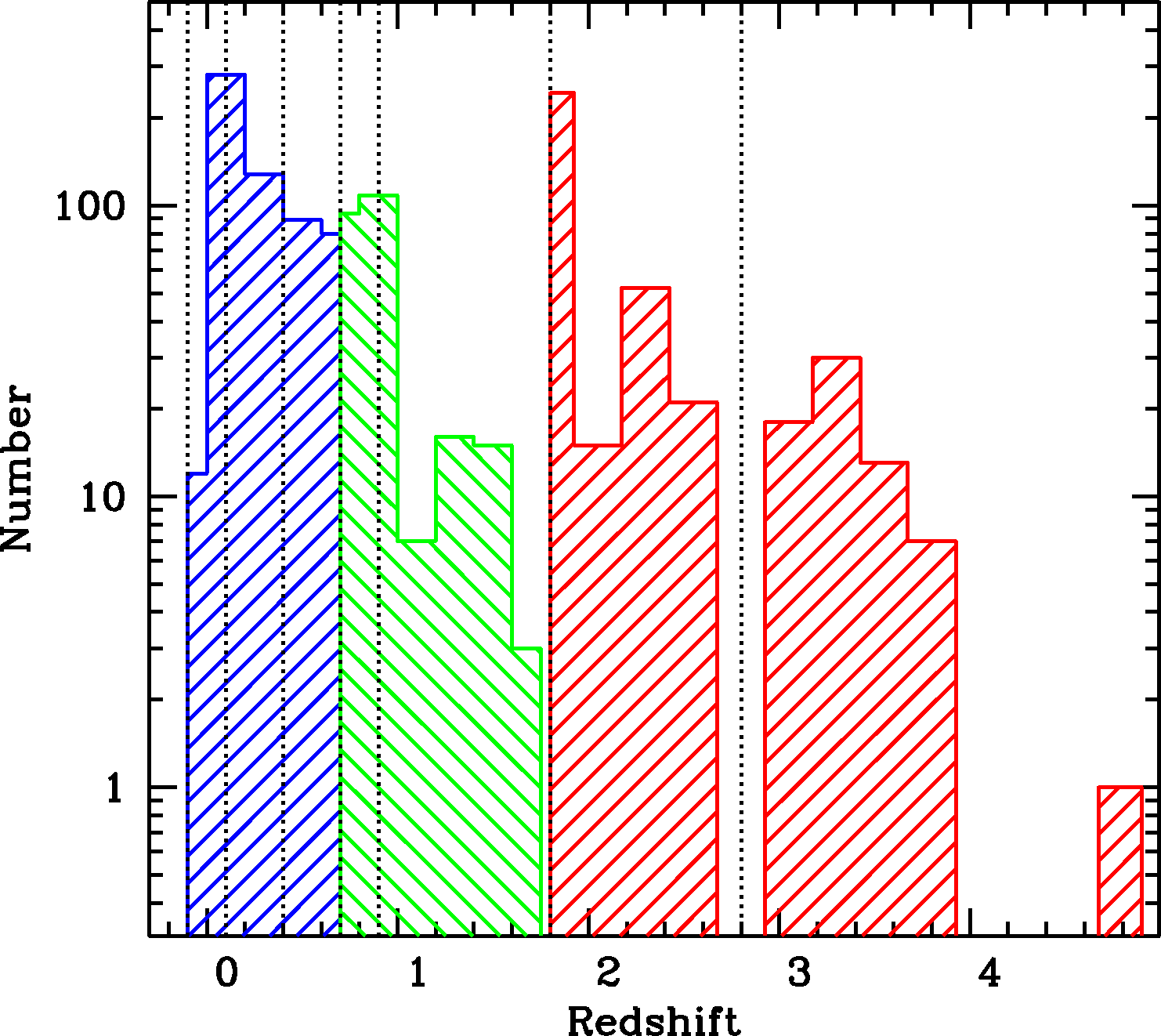
The redshift distribution of the MEGA dataset is shown in Fig. 1, together with the 7 redshift bins that will be used throughout the paper. As mentioned above, Table LABEL:tab:samples gives the characteristics of the 19 individual samples comprising the MEGA dataset; there is a total of 990 galaxies from $z\simeq 0$ to $z\sim 3.7$ (and LnA1689$-$2 in the AMAZE sample at $z\,=\,4.87$).

3 Metallicity calibrations

Oxygen abundance O/H is typically used as a proxy for metallicity in emission-line galaxies. Because the ionized gas in Hii regions at lower metal abundance is hotter (as measured by electron temperature, T${}_{\rm e}$), the preferred technique to establish O/H is to measure T${}_{\rm e}$ and the physical conditions in the ionized plasma. In this “direct-temperature” or “T${}_{\rm e}$” method, the T${}_{\rm e}$ of the ionized gas is derived from the ratio of the [Oiii] $\lambda$4363 auroral line to lower-excitation lines ([Oiii] $\lambda$4959, 5007); such flux ratios are sensitive to temperature because the auroral and strong lines originate from different excitation states (second and first excited states, respectively). Because the oxygen transitions are collisionally excited, the relative population of the excited states depends on T${}_{\rm e}$. Thus, the strengths of these forbidden lines, combined with the measurement of T${}_{\rm e}$ and density in the nebula, can be converted to an abundance, relative to hydrogen, after correcting for unseen phases of ionization (e.g., osterbrock06).

Although the T${}_{\rm e}$ method is more directly related to metallicity, the auroral lines are weak and often difficult to detect, especially at high metallicity. Thus, “strong-line” methods are more generally used to estimate O/H, especially in metal-rich objects and at high redshift. It is necessary to calibrate these methods, either using theoretical photoionization models (e.g., kewley02, hereafter KD02), or measurements of T${}_{\rm e}$ (e.g., pettini04, hereafter PP04), or a combination of the two (e.g., denicolo02, hereafter D02). Despite the best efforts to correctly cross calibrate these methods over a wide range of physical conditions, there remain large discrepancies, as high as 0.6 dex in log(O/H) (e.g., kewley08, and references therein). Thus to correctly assess metal content and its evolution with redshift, it is necessary to apply a common metallicity calibration to the samples under discussion.

In nearby galaxies where spectra can be obtained with sufficient signal-to-noise, the T${}_{\rm e}$ method is generally used. As mentioned above, the most widely used auroral T${}_{\rm e}$ diagnostic line is [Oiii] $\lambda$4363 because of its relative ease of observation, high abundance of emitting ions, and notable strength in the low- and intermediate-metallicity regime (i.e., below solar metallicity). However, there are several potential problems with the T${}_{\rm e}$ method based on [Oiii]:

1. Metallicities derived from collisionally-excited lines (CELs) such as [Oiii] can be underestimated when temperature fluctuations inside the nebula are present but neglected. The assumption of a single average CEL temperature for the whole nebula, usually higher than the temperature derived from the Balmer discontinuity, tends to lead to an underestimate of the abundances (e.g., peimbert67; stasinska05; bresolin07; perez10; pena12).

2. Additional problems also plague the T${}_{\rm e}$ method including possible non-Boltzmann electron distributions (e.g., nicholls12; binette12; nicholls13); depletion of oxygen onto dust grains (e.g., peimbert10; pena12); and potential shock waves within the nebulae (e.g., binette12).

3. Finally, recent results suggest that metallicities derived from [Oiii] may be more unreliable than those from other auroral lines such as [Siii] $\lambda$6312 and [Nii] $\lambda$5755 (e.g., berg15); however, these lines are even more difficult than [Oiii] to measure in distant galaxies.

An alternative to the use of T${}_{\rm e}$-diagnostic lines can be the derivation of abundances from optical recombination lines (ORLs), because of their reduced emissivity dependence on density and temperature. Abundances derived from the ratio of the intensity of ORLs tend to be systematically higher than those from CELs (e.g. peimbert93; liu95; liu01; tsamis04; ge07). However, such differences may arise from the relation of the ORL abundances to small H-deficient portions of the regions, while the CEL-based metallicities are more representative of the whole nebula (see, e.g., liu00). Moreover, such lines are extremely faint, thus requiring very high signal-to-noise spectra that are currently available only for the Galaxy and the Local Group (e.g., blanc15).

There are also, perhaps more severe, problems with “strong-line” methods, and the simplifying assumptions made for photoionization model calibrations (e.g., photoionization structure, geometry, stellar age: see moustakas10, for a thorough discussion). As for the T${}_{\rm e}$ method, there may also be systematic discrepancies due to the metallicity-dependent correction for the depletion of oxygen onto dust grains (e.g., peimbert10). Ultimately, the T${}_{\rm e}$ method (with [Oiii]) is generally considered to be the most viable, given the limitations with other techniques.

Thus, to ensure the best possible comparison among different samples that rely on different O/H calibrations, it is advantageous to use the strong-line calibration method that most closely resembles values inferred from oxygen-based T${}_{\rm e}$-method estimations. According to the results of andrews13, who used a stacking technique to measure the oxygen abundances of $\sim$200 000 star-forming galaxies from the SDSS to enhance the signal-to-noise ratio of the weak [Oiii] $\lambda$4363 line, there are three such methods: PP04 (both [Nii] and [Oiii]$+$[Nii]-based: hereafter PP04N2, PP04O3N2) and D02. Over the metallicity and M${}_{*}$ range covered by their calculations of various strong-line methods (see Fig. 10 of andrews13), the discrepancies between the T${}_{\rm e}$ method and these three methods are $\la$0.1 dex in 12$+$log(O/H).

Thus, in what follows, where there are no direct-T${}_{\rm e}$ estimates, we have applied the transformations given by kewley08 to convert the original strong-line O/H calibrations for the MEGA dataset (and SDSS10 sample) to the calibrations by D02 and PP04 (PP04N2, PP04O3N2). As reported in Table LABEL:tab:samples, the original O/H calibrations include: KD02 (kewley02; cresci12; mannucci10; troncoso14); KK04 (kobulnicky04; kennicutt11; henry13; xia12); M91 (mcgaugh91; marble10); PP04N2, PP04O3N2 (pettini04; shapley04; shapley05; liu08; yabe12; zahid14; steidel14); and T04 (tremonti04; delosreyes15).

Figure 2: Mass-metallicity relation over redshifts from $z\sim 0$ to $z\ga 3.3$, binned as described in the text. The solid (black) curve (labeled $z\sim 0$) corresponds to the fit to SDSS10 (with stacked T${}_{\rm e}$ metallicity determinations) by andrews13, and the dotted (grey) curves to the polynomial fits by maiolino08 with the KD02 calibration at $z\approx 0.07$, $z\approx 0.7$, $z\approx 2.2$, and $z\approx 3.5$. The O/H calibration for all galaxies is PP04N2 as described in the text. Samples are labeled according to the legend in the lower rightmost panel, except for $z\ \approx\ 0$ which are: LVL as small open circles (colors correspond to Hubble types with late types (T$\geq$8) as cyan, 5$\leq$T$<$8 as blue, 3$\leq$T$<$5 as magenta, T$<$3 as red); KINGFISH as (orange) $+$; engelbracht08 as (purple) filled triangles; hunt10 as (blue) filled squares. The stacked samples (yabe14; zahid14) at $z\approx 1$ are not plotted.

Figure 3: Specific SFR vs. M${}_{*}$ (main sequence of star formation) over redshifts from $z\sim 0$ to $z\ga 3.3$, binned as described in the text. The solid (black) curve (labeled $z\sim 0$) corresponds to the fit to the LVL$+$KINGFISH samples, and the dotted (grey) curves to the formulation of dependence with M${}_{*}$ and $z$ by speagle14 for $z\approx 0.6$, $z\approx 1.3$, $z\approx 2.3$, and $z\approx 3.3$. Symbols are as in Fig. 2, and the stacked samples (yabe14; zahid14) are not plotted.

4 Scaling relations and the fundamental plane

The MEGA dataset comprises three parameters (pseudo-observables, as they are not directly observed): nebular oxygen abundance (12$+$log(O/H)), stellar mass (M${}_{*}$), and SFR. As discussed in the Introduction, these three parameters are mutually correlated, although O/H trends flatten at high M${}_{*}$ (and high O/H). Here we discuss the scaling relations of the three parameters: the mass-metallicity relation, MZR, the “main sequence” of star formation, SFMS, and the correlation (at least at $z\sim 0$) between sSFR and metallicity.

Figure 4: Specific SFR vs. 12$+$log(O/H) over redshifts from $z\sim 0$ to $z\ga 3.3$, binned as described in the text. The solid (black) line corresponds to the fit to the best-fit slope for the MEGA sample at $z\sim 0$, and the dotted (grey) lines to the prediction of the redshift variation assuming the increase in sSFR given by speagle14 (from $z\sim 0.6$, $z\sim 1.3$, $z\sim 2.3$, $z\sim 3.3$) of the Fundamental Plane for these two parameters described in Sect. 4.2. As in Fig. 2, the O/H calibration for all galaxies is PP04N2 as described in the text. Symbols are as in Fig. 2, and the stacked samples (yabe14; zahid14) are not plotted.

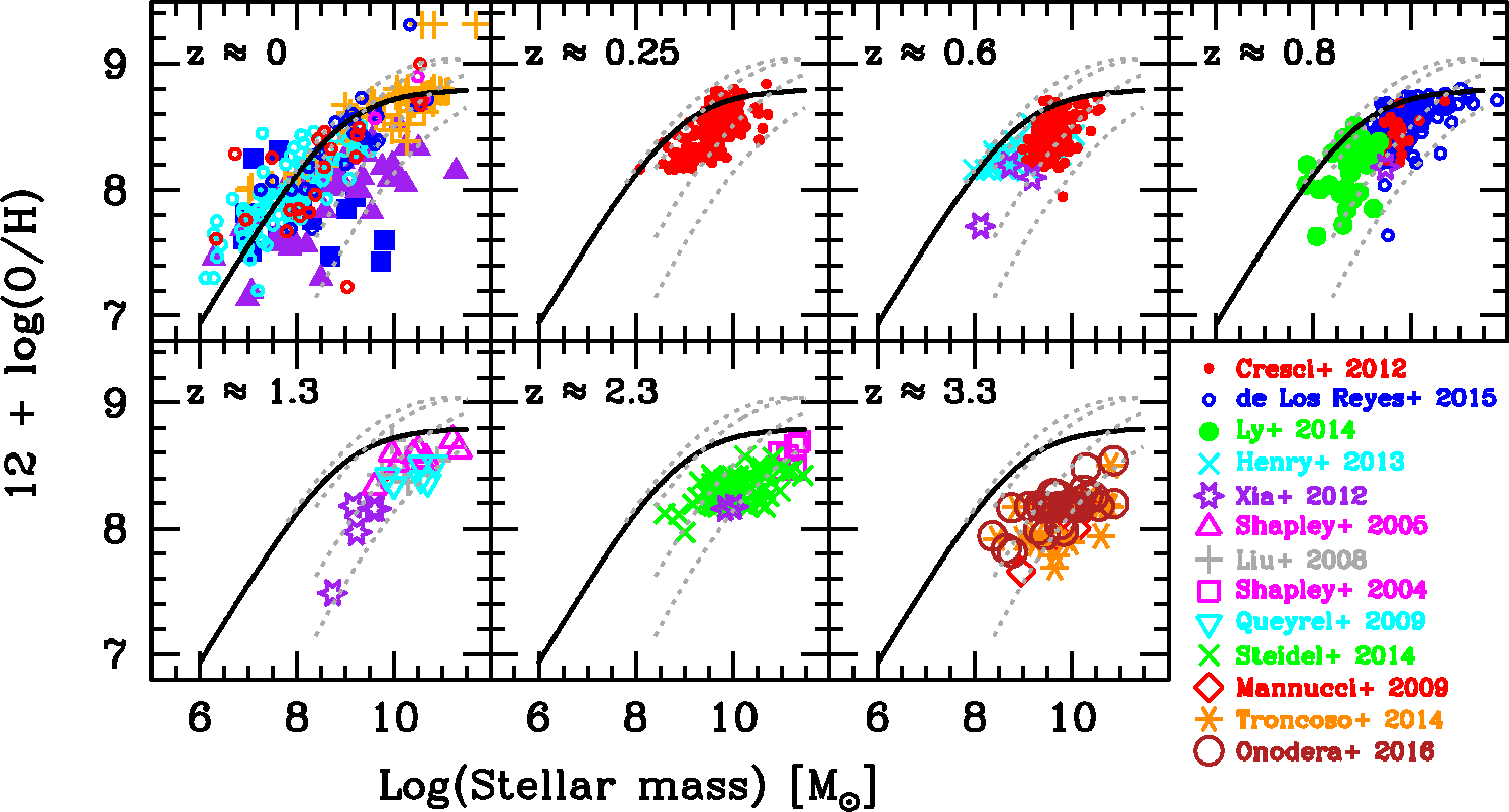
The MZR with the PP04N2 O/H calibration for different redshift bins is shown in Fig. 2. The solid curve shows the T${}_{\rm e}$-method MZR derived by andrews13 which well approximates the MEGA dataset at $z\approx 0$. The dotted grey curves represent the polynomial fits given by maiolino08 for the KD02 calibration; at high M${}_{*}$, these curves fail to capture the T${}_{\rm e}$-derived (or PP04N2) metallicities because of the different O/H calibration. As virtually all previous work suggests, the different panels illustrate that as $z$ increases, at a given M${}_{*}$ metallicity decreases. However, at $z\approx 0$ for a given M${}_{*}$, the starburst and BCD samples tend to be more metal-poor than the LVL and KINGFISH galaxies; they behave more like galaxies at $z\ga 1$ than like galaxies in the Local Universe, presumably because of their higher sSFR.

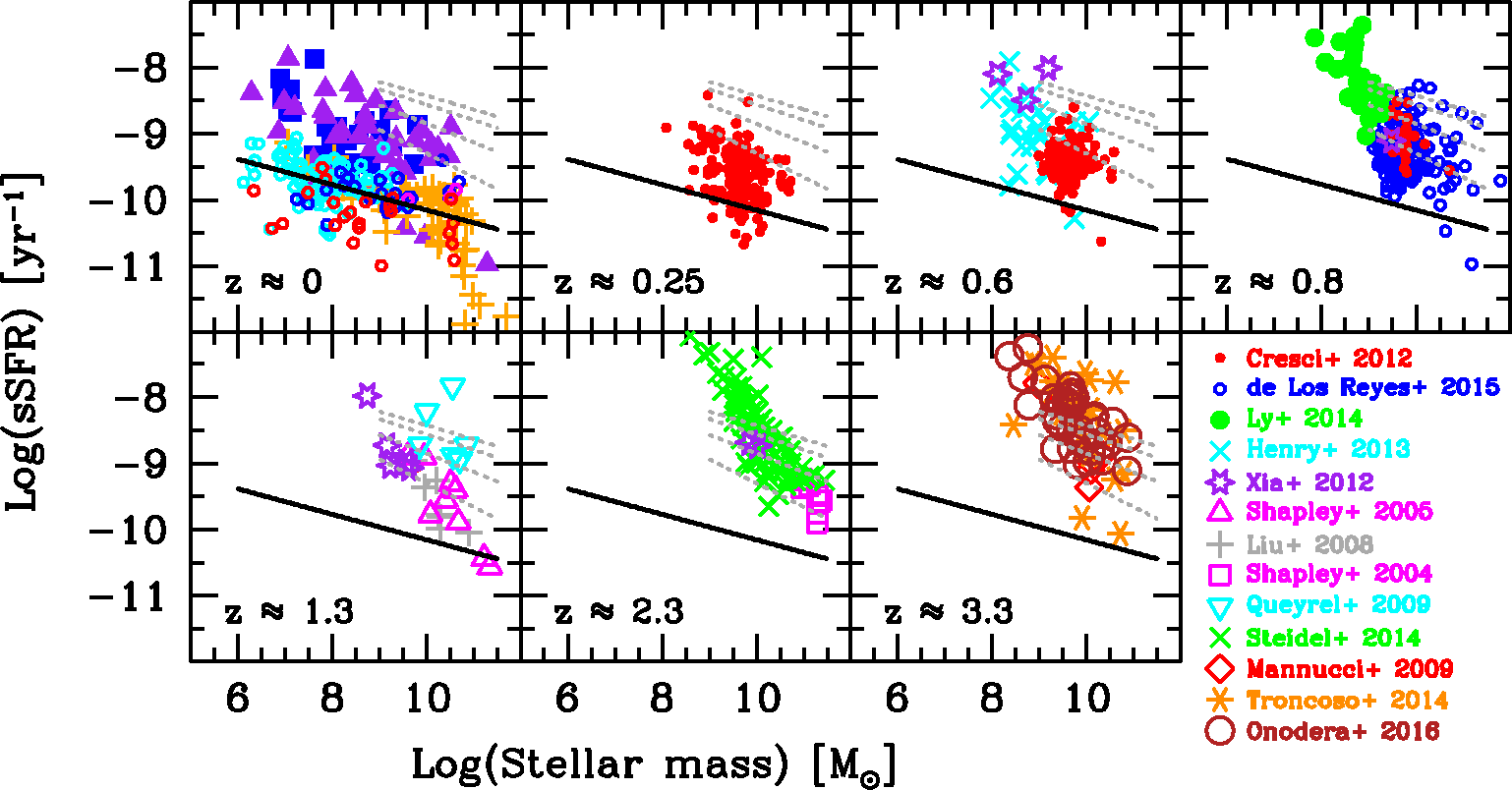
The high sSFRs in the starburst and BCD $z\approx 0$ samples are more clearly seen in Figure 3, which shows the SFMS, or sSFR plotted against M${}_{*}$. The solid line shows the SFMS calibrated with the LVL$+$KINGFISH samples, having a slope of $-0.19\,\pm\,0.02$, roughly consistent with that ($-0.23$) found by elbaz07 for $z\sim 0$ galaxies. The dashed grey lines correspond to the speagle14 formulation for SFR as a function of cosmic time (we have calculated cosmic age for representative redshifts and plotted the result). The slope by speagle14 at $z\ga 2$ is similar to what we find for the Local Universe, which however is shallower (steeper in SFR-M${}_{*}$ space) than their value for $z\sim 0$. Fig. 3 illustrates that as redshift increases, for a given M${}_{*}$, sSFR also increases; galaxies that would be main-sequence galaxies at $z\ga 1$ are starbursts if found at $z\approx 0$. However, it is also seen from the figure that the individual high-$z$ samples do not clearly follow the SFMS; this is almost certainly due to selection effects and will be further discussed in Sect. LABEL:sec:massvariation. Because of the difficulty in measuring metallicities in high-$z$ emission-line galaxies, flux limits for spectroscopy impose a commensurate limit in SFRs.

Figure 5: SDSS10 galaxies: 12$+$log(O/H) plotted against (log of) M${}_{*}$. The three panels correspond to number densities of 12$+$log(O/H) (with the three O/H calibrations) and M${}_{*}$. In each panel, the solid curves correspond to the mass-metallicity relation taken from andrews13 for stacked O/H direct-temperature metallicity determinations as also shown in Fig. 2. The dashed curves show instead the relation of the form used by andrews13 but fit to the SDSS10 data used here.

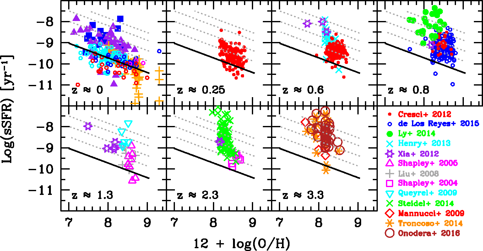
The third correlation between sSFR and O/H is shown in Figure 4. As in previous figures, the solid line gives the local calibration on the LVL$+$KINGFISH and the dotted grey lines show the redshift trend for O/H expected for the higher SFR as predicted by the FPZ (see Sect. 4.2). The SFRs of the local starbursts and BCDs are higher at a given O/H, relative to the other local samples; again, they are more similar to galaxies at $z\ga 1$ than to typical local populations. Similarly to the behavior of the MEGA dataset for the SFMS, the LVL$+$KINGFISH galaxies show a well-defined correlation between sSFR and O/H, but the correlation disappears for the higher-redshift samples.

The main point of this third correlation is that, at least locally, the three psuedo-observables, 12$+$log(O/H), SFR, and M${}_{*}$ are mutually interdependent. This makes it difficult to determine which is the primary parameter(s) driving the relations, and it this point which we explore below in Sect. 4.2.

4.1 The SDSS10 relations

Similar correlations are found for the SDSS10 galaxies, although the range in M${}_{*}$, O/H, and sSFR is smaller than in the MEGA dataset. Nevertheless, over the limited parameter range the sheer number statistics afford precise determinations of scaling relations and fitting functions which will be important for constraining our models.

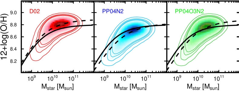
Fig. 5 gives the MZR for the three O/H calibrations of SDSS10 sample, transformed from the original KD02. The solid curves, also shown in Fig. 2, give the MZR for the direct-method O/H as found by andrews13, while the dashed ones are functions of the same form but fit to the SDSS10 dataset itself. The PP04 calibrations (middle and right panels) are, on average, the best approximation to the direct-method O/H curve, although at 12$+$log(O/H) $\la$8.5, the D02 calibration is superior. In any case, the functional MZR form used by andrews13 does not well approximate the SDSS10 data at low mass or low metallicities. The low-mass, low-metallicity linear portion of the data has a slope of $\sim 0.38\,\pm\,0.003$, similar to the MZR curve, but the latter is offset to higher masses.

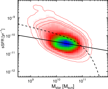
The SFMS of the SDSS10 data is shown in Fig. 6; the solid line corresponds to the linear regression for the LVL$+$KINGFISH galaxies (also shown in Fig. 3) and the dashed curve to the Schechter-like functional form fitted by salim07. Although this last captures the low- and high-mass ends of the SDSS10 data, it does not pass through the region with the highest density (blue colors in Fig. 6). This could have something to do with the different ways that SFR is calculated; salim07 used FUV while mannucci10 used extinction-corrected H$\alpha$. Nevertheless, the LVL$+$KINGFISH regression well approximates this behavior, implying that the SFR derivation is probably not the cause of the discrepancy. The third correlation, between sSFR and 12$+$log(O/H) is not shown for the SDSS10 data; it shows a similar behavior to the MEGA sample.

Figure 6: SDSS10 galaxies: sSFR plotted against M${}_{*}$. The color scale corresponds to the number densities of the two parameters. The solid curve gives the linear SF “main sequence” regression to the LVL$+$KINGFISH samples (also shown in Fig. 3), and the dashed curve to the Schechter function fitted by salim07.

4.2 A planar approximation to scaling relations

At high M${}_{*}$ and O/H, both the MZR and SFMS inflect and flatten (e.g., tremonti04; noeske07; whitaker14; lee15; gavazzi15). However, for M${}_{*}$ below a certain threshold, M${}_{*}$$\leq 3\times 10^{10}$ $M_{\odot}$, roughly the “turn-over mass” (tremonti04; wyder07), the relations among the variables are approximately linear. We propose that, at high M${}_{*}$ and O/H, the inflections the MZR and the SFMS compensate one another, and hypothesize that even above this inflection threshold, the trends in M${}_{*}$, O/H, and SFR can be approximated by linear relations. Consequently, as discussed above, these observationally-defined variables could define a plane which, given the relatively large scatters in the SFMS, the MZR, and the SFR-O/H relation, is not viewed in the best projection. Because the three parameters are mutually correlated, it is important to determine which of the three is the most fundamental, and whether or not the planar approximation is sufficient to describe the data. This can be readily accomplished through a Principal Component Analysis (PCA, e.g., hunt12).

The MEGA dataset is a significant improvement on the sample studied by hunt12, and is particularly well suited for such an analysis. In particular, the MEGA dataset triples the number of galaxies at $z\ga 2-3$ with respect to hunt12. It spans almost two orders of magnitude in metallicity (12$+$log(O/H) = 7.1 to $\sim 9$), a factor of $\sim 10^{6}$ in SFR ($\sim 10^{-4}\leq$ SFR $\leq\,\sim 10^{2}$ $M_{\odot}$ yr${}^{-1}$), and a factor of $\sim 10^{5}$ in stellar mass ($\sim 10^{6}\leq$ M${}_{*}$ $\leq\,\sim 10^{11}$ $M_{\odot}$); moreover it includes galaxies at redshifts from $z\sim 0-3.8$ (see Fig. 1). Other samples previously analyzed to find scaling relations cover much smaller parameter ranges: typically less than a decade in metallicity (12$+$log(O/H)$\geq$8.4), a factor of $\sim$200 in SFR ($\sim$0.04$\la$ SFR$\la 6$ $M_{\odot}$ yr${}^{-1}$), and roughly 2 orders of magnitude in stellar mass (M${}_{*}$$\ga 10^{9}$ $M_{\odot}$) (e.g., tremonti04; mannucci10; laralopez10; yates12). Because more than 50% of the MEGA dataset has $z>0.5$, and it includes galaxies at redshift $z\ga 3.5$, we can test the assumption that the relations among the observationally-defined variables are redshift invariant.

Figure 7: Top panel: FPZ projection of O/H for all O/H calibrations of the MEGA dataset as described in the text. All galaxies are shown (in gray intensity and contours), including those with M${}_{*}$$\geq 3\times 10^{10}$ $M_{\odot}$; colored filled circles correspond to galaxies with $z\geq 2$. The dashed lines give the identity relation. Bottom panel: histograms of FPZ residuals from the identity relation. The grey histograms show all galaxies, while the (lower-amplitude) colored ones correspond to galaxies with $z\geq 2$. The heavy dashed lines give the Gaussian fit of the residuals (including the separate fit to the galaxies with $z\geq 2$); the $\sigma$ values in the upper left corner of each panel correspond to the mean residuals for all galaxies. The width of the best (PP04N2) residual distribution over all redshifts is $\sim$0.16 dex (see middle panels).

4.3 PCA of the MEGA and SDSS10 samples

We have therefore performed a PCA for all three O/H calibrations of the MEGA dataset without imposing a limit in M${}_{*}$ (c.f., hunt12). A PCA diagonalizes the 3D covariance matrix, thus defining the orientation of the parameter space which minimizes the covariance. The orientation is contained in the eigenvectors which are, by definition, mutually orthogonal. If the 3D space formed by the three psuedo-observables is truly planar, we would expect most of the variance to be contained in the first two eigenvectors (the orientation of the plane); for the third eigenvector, perpendicular to the plane, the variance should be very small.

Independently of the O/H calibration, the PCA shows that the set of three observables truly defines a plane; $\ga$98% of the total variance is contained in the first two eigenvectors. Most (87%) of the variance is contained in the first eigenvector alone (or Principal Component, PC), PC1; it is dominated by SFR, with M${}_{*}$ contributing slightly less, and O/H giving only a marginal contribution. PC2, the second eigenvector, holds 10$-$11% of the variance, and is dominated by M${}_{*}$, followed by SFR, and as in PC1, with O/H again only marginal. The smallest fraction of the variance ($\sim 1.5-1.8$%) is contained in the third eigenvector, PC3, which is dominated by O/H; the implication is that O/H is the most dependent parameter, governed almost completely by M${}_{*}$ and SFR. Moreover, this means that the 3D space defined by O/H, SFR, and M${}_{*}$ is degenerate; because of the mutual correlations of the psuedo-observables, only two parameters are required to describe the properties of the galaxies.

We have also performed a PCA of the SDSS10 galaxies, and obtained similar results: namely, the third eigenvector, PC3, the one dominated by O/H, contains the smallest fraction of the variance. The residuals of 0.05$-$0.06 dex are comparable to that obtained by the FMR formulation by mannucci10.

That star-forming galaxies form a plane in O/H, SFR, and M${}_{*}$ is not a new result. laralopez10 concluded that the 3D space of O/H, SFR, and M${}_{*}$ of $\sim$ 33 000 SDSS galaxies could be represented as a plane but used a regression analysis rather than a PCA (although see laralopez13). hunt12 derived a PCA for a dataset similar to ours, although dominated by LCGs, and also concluded that a 2D plane was sufficient to describe the 3D dataset.

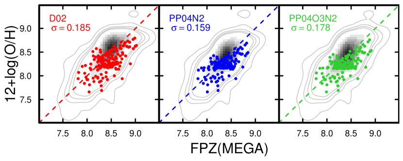
As in the Introduction, we will refer to the resulting 2D plane as the FPZ (Fundamental Plane in metallicity). The FPZ for the MEGA dataset is shown in the top panel of Figure 7 where we have plotted 12$+$log(O/H) vs. the equation that results from equating PC3 (PP04N2) to zero (see Table LABEL:tab:fpzfmr for the other O/H calibrations):

$$12+\log(O/H)=-0.14\,{\rm log(SFR)}+0.37\,{\rm log(M_{*})}+4.82\ \$$ (1)

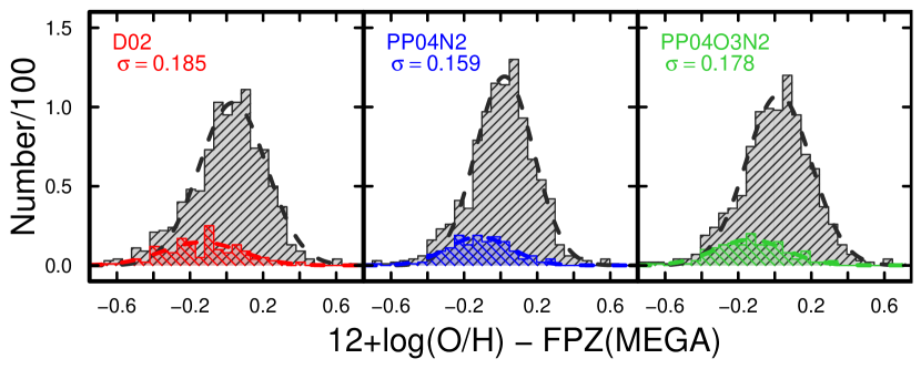
The bottom panel of Fig. 7 shows the residuals from the FPZ for the different O/H calibrations. For PP04N2, they are well approximated by a Gaussian with a $\sigma\,=\,0.16$, corresponding to $\la$45% uncertainty; the other two O/H calibrations (D02, PP04O3N2) give similar results, although slightly larger (see Table LABEL:tab:fpzfmr). The residuals of the FPZ relation are independent of redshift to within 0.16 dex, the overall uncertainty; nevertheless the different symbols plotted in the top panel (and the different histograms in the bottom one) suggest some slight deviation with redshift which we will explore in Sect. LABEL:sec:fpzinvariance.

Because of the turnover of the MZR and SFMS at high stellar masses, our assumption of linearity in the FPZ could also produce a residual correlation with M${}_{*}$. We have investigated this possibility and found that the FPZ residuals and (log)M${}_{*}$ are uncorrelated; the mean residuals of the regression are $\sim$0.16 dex (for the PP04 calibration), the same as those of the FPZ itself. Moreover, the slope of the FPZ residuals vs. (log)M${}_{*}$ is zero to within the uncertainties ($-0.015\,\pm\,0.01$). Thus, our hypothesis that the inflections in the MZR and SFMS compensate one another is apparently justified; the curvature in the MZR can be adequately accommodated by the increasing SFRs at high M${}_{*}$, at least to within the uncertainties of our data.

The FPZ dispersion of $\sim 0.16-0.18$ dex for the MEGA dataset is higher than that found by tremonti04 for the MZR defined by 53 000 galaxies from the SDSS (0.1 dex), and also higher than the FMR (0.06 dex) found for the SDSS10 sample by mannucci10. However, as shown in Table LABEL:tab:fpzfmr, the SDSS10 data span limited ranges in O/H, SFR, stellar mass (and redshift) relative to the parameter space covered by the MEGA data. The mean and standard deviation of (log) stellar mass for the SDSS10 sample is $10.26\pm 0.41$ $M_{\odot}$, while the comparable mean, standard deviation for MEGA is $9.44\pm 0.93$ $M_{\odot}$; (log) SFR shows a similar pattern: $-0.04\pm 0.43$ $M_{\odot}$ yr${}^{-1}$ for SDSS10 compared to $0.16\pm 1.12$ $M_{\odot}$ yr${}^{-1}$ for MEGA. Thus, the higher dispersion in the MEGA FPZ is not surprising despite the many more galaxies in SDSS.

The value of the FPZ dispersion is lower than the scatter of the MZR for $\sim$20 000 VVDS galaxies within individual redshift bins from $z\sim 0.3-0.9$ ($\sim$0.20 dex, lamareille09). The FPZ dispersion for the $\sim$1000 galaxies studied here is only slightly higher than that found for the MZR of 25 nearby dwarf galaxies (0.12 dex, lee06), a sample dominated by low-mass galaxies. It is also only slightly higher than the rms scatter of 0.12 dex found by henry13 for 18 galaxies at $z\sim 0.6$ in the mass range dex(8.5)$\leq$M${}_{*}$$\leq$dex(9.0). Because the dispersion in the MZR is found to increase with decreasing M${}_{*}$ (tremonti04; mannucci11), a $\sigma$ of 0.16 dex is a reasonable value, given the broad parameter space covered by our dataset.

4.4 Comparison with the FMR

Table 2: FPZ and FMR applied to MEGA and SDSS datasets${}^{\mathrm{a}}$

Sample	Calibration	$\sigma_{\rm fit}^{\mathrm{b}}$	Offset(fit)${}^{\mathrm{b}}$	$\langle$12$+$log(O/H)$\rangle$${}^{\mathrm{c}}$	$\langle$Log(SFR)$\rangle$${}^{\mathrm{c}}$	$\langle$Log(M${}_{*}$)$\rangle$${}^{\mathrm{c}}$	12$+$log(O/H) =
(1)	(2)	(3)	(4)	(5)	(6)	(7)	(8)
MEGA FPZ applied to the MEGA and SDSS10 datasets
MEGA	D02	0.185	0.03	$8.422\,\pm\,0.33$	$0.159\pm 1.12$	$9.440\,\pm\,0.93$	$-0.17\ s+0.44\ m+4.33$
MEGA	PP04N2	0.159	0.02	$8.332\,\pm\,0.30$	$0.159\pm 1.12$	$9.440\,\pm\,0.93$	$-0.14\ s+0.37\ m+4.82$
MEGA	PP04O3N2	0.178	0.03	$8.355\,\pm\,0.32$	$0.159\pm 1.12$	$9.440\,\pm\,0.93$	$-0.16\ s+0.41\ m+4.48$
SDSS10	D02	0.102	$-0.04$	$8.768\,\pm\,0.09$	$-0.038\pm 0.43$	$10.263\,\pm\,0.41$	As above for D02.
SDSS10	PP04N2	0.080	$-0.004$	$8.660\,\pm\,0.11$	$-0.038\pm 0.43$	$10.263\,\pm\,0.41$	As above for PP04N2.
SDSS10	PP04O3N2	0.088	$-0.01$	$8.709\,\pm\,0.12$	$-0.038\pm 0.43$	$10.263\,\pm\,0.41$	As above for PP04O3N2.
FMR${}^{\mathrm{d}}$ applied to the MEGA and SDSS10 datasets
							12$+$log(O/H) =
							$\mu_{0.32}<$9.5 $M_{\odot}$${}^{\mathrm{e}}$	$\mu_{0.32}\geq$9.5 $M_{\odot}$${}^{\mathrm{e}}$
(1)	(2)	(3)	(4)	(5)	(6)	(7)	(8)	(9)
MEGA	D02	0.175	$-0.14$	$8.422\,\pm\,0.33$	$0.159\pm 1.12$	$9.440\,\pm\,0.93$	$-0.16\ s+0.51\ m+3.83$	$-13.8+4.17m-1.34s+0.12m\,s-0.19m^{2}-0.054s^{2}$
MEGA	PP04N2	0.168	$-0.25$	$8.332\,\pm\,0.30$	$0.159\pm 1.12$	$9.440\,\pm\,0.93$	$-0.16\ s+0.51\ m+3.83$	$-13.8+4.17m-1.34s+0.12m\,s-0.19m^{2}-0.054s^{2}$
MEGA	PP04O3N2	0.181	$-0.22$	$8.355\,\pm\,0.32$	$0.159\pm 1.12$	$9.440\,\pm\,0.93$	$-0.16\ s+0.51\ m+3.83$	$-13.8+4.17m-1.34s+0.12m\,s-0.19m^{2}-0.054s^{2}$
							12$+$log(O/H) =
							$\mu_{0.32}<$10.2 $M_{\odot}$${}^{\mathrm{e}}$	$\mu_{0.32}>$10.5 $M_{\odot}$${}^{\mathrm{e}}$
(1)	(2)	(3)	(4)	(5)	(6)	(7)	(8)	(9)
SDSS10	D02	0.05	$-0.25$	$8.768\,\pm\,0.09$	$-0.038\pm 0.43$	$10.263\,\pm\,0.41$	$-0.15\ s+0.47\ m+4.20$	$9.07$
SDSS10	PP04N2	0.05	$-0.34$	$8.660\,\pm\,0.11$	$-0.038\pm 0.43$	$10.263\,\pm\,0.41$	$-0.15\ s+0.47\ m+4.20$	$9.07$
SDSS10	PP04O3N2	0.06	$-0.28$	$8.709\,\pm\,0.12$	$-0.038\pm 0.43$	$10.263\,\pm\,0.41$	$-0.15\ s+0.47\ m+4.20$	$9.07$

${}^{\mathrm{a}}$ Applying the FPZ and the FMR to the entire mass range according to Eqn. 1. In the equations of Cols. (8,9), $s$ corresponds to Log(SFR) and $m$ to Log(M${}_{*}$). The sense of the residuals is 12$+$log(O/H)(data) $-$ 12$+$log(O/H)(FPZ,FMR).

${}^{\mathrm{b}}$ Standard deviation $\sigma$ and offset of the FPZ or FMR residuals (e.g., Fig. 7).

${}^{\mathrm{c}}$ Means and standard deviations of the samples.

${}^{\mathrm{d}}$ We took the FMR for the MEGA sample from the extension to lower M${}_{*}$ by mannucci11, and for SDSS10 from mannucci10; for both we have converted their recipes with $\mu_{0.32}$ to the multiplicative formulation as for the FPZ.

${}^{\mathrm{e}}$ The divisions for the FMR are in $\mu_{0.32}$, where $\mu_{0.32}\,\equiv\,$Log(M${}_{*}$) $-$ 0.32 Log(SFR) (mannucci10).