KCL-PH-TH/2016-52, CERN-PH-TH/2016-185

KIAS–P16059, UMN–TH–3601/16, FTPI–MINN–16/23

The Super-GUT CMSSM Revisited

John Ellis^1,2, Jason L. Evans³, Azar Mustafayev⁴,

Natsumi Nagata⁴ and Keith A. Olive^4
1Theoretical Physics and Cosmology Group, Department of Physics,
King’s College London, Strand, London WC2R 2LS, UK
²Theoretical Physics Department, CERN, CH-1211 Geneva 23, Switzerland
³School of Physics, KIAS, Seoul 130-722, Korea
⁴William I. Fine Theoretical Physics Institute, School of Physics and Astronomy,
University of Minnesota, Minneapolis, MN 55455, USA

Abstract

We revisit minimal supersymmetric SU(5) grand unification (GUT) models in which the soft supersymmetry-breaking parameters of the minimal supersymmetric Standard Model (MSSM) are universal at some input scale, $M_{in}$, above the supersymmetric gauge coupling unification scale, $M_{GUT}$. As in the constrained MSSM (CMSSM), we assume that the scalar masses and gaugino masses have common values, $m_{0}$ and $m_{1/2}$, respectively, at $M_{in}$, as do the trilinear soft supersymmetry-breaking parameters $A_{0}$. Going beyond previous studies of such a super-GUT CMSSM scenario, we explore the constraints imposed by the lower limit on the proton lifetime and the LHC measurement of the Higgs mass, $m_{h}$. We find regions of $m_{0}$, $m_{1/2}$, $A_{0}$ and the parameters of the SU(5) superpotential that are compatible with these and other phenomenological constraints such as the density of cold dark matter, which we assume to be provided by the lightest neutralino. Typically, these allowed regions appear for $m_{0}$ and $m_{1/2}$ in the multi-TeV region, for suitable values of the unknown SU(5) GUT-scale phases and superpotential couplings, and with the ratio of supersymmetric Higgs vacuum expectation values $\tan\beta\lesssim 6$.

August 2016

1 Introduction

There have been many phenomenological studies of the minimal supersymmetric (SUSY) extension of the Standard Model (MSSM) that assume some degree of universality for the soft supersymmetry-breaking scalar and gaugino masses, $m_{0}$ and $m_{1/2}$, and the trilinear soft supersymmetry-breaking parameters $A_{0}$. Scenarios in which these parameters are universal at the supersymmetric grand unification (GUT) scale, $M_{GUT}$, called the constrained MSSM (CMSSM) [1, 2, 3, 4, 5, 6], have been particularly intensively studied, usually assuming that the lightest supersymmetric particle (LSP) is a neutralino, which is stable because of the conservation of $R$-parity [7], and provides (all or some of) the cosmological cold dark matter. These and other GUT-universal models are under strong pressure from LHC data [5, 6, 8, 9, 10, 11, 12, 13, 14, 15, 16, 17, 18], in particular, the notable absence of missing transverse energy signals at the LHC [19, 20], with the measurement of the Higgs mass [21, 22], $m_{h}$, providing an additional important constraint.

Fewer studies have been performed for scenarios in which the soft supersymmetry-breaking parameters are universal at some other scale $M_{in}\neq M_{GUT}$, which might be either below the GUT scale (so-called sub-GUT or GUT-less scenarios [23, 11, 18]) or above the GUT scale (so-called super-GUT scenarios [24, 25, 26]). For example, in our current state of confusion about the possible mechanism of supersymmetry breaking, and specifically in the absence of a convincing dynamical origin at $M_{GUT}$, one could well imagine that the universality scale $M_{in}$ might lie closer to the Planck or string scale: $M_{in}>M_{GUT}$.

When studying such super-GUT scenarios, there appear additional ambiguities beyond those in the conventional CMSSM. What is $M_{in}$? Which GUT model to study? What are its additional parameters? How much additional freedom do they introduce? In parallel, once one commits to a specific GUT model, one must also consider the constraint imposed by the absence (so far) of proton decay [27]. In order to minimize the ambiguities and the number of additional GUT parameters, we study here the minimal supersymmetric SU(5) GUT [28].

It is well known that the length of the proton lifetime is a significant challenge for this model [29, 30], and one of the principal new ingredients in this paper, compared to previous studies of super-GUT CMSSM models, is the incorporation of this constraint in our exploration of the model parameter space. Another improvement on previous super-GUT CMSSM studies is the incorporation of LHC constraints, of which the measurement of the Higgs mass turns out to be the most relevant.

We find regions of the soft supersymmetry-breaking parameters $m_{0}$, $m_{1/2}$, $A_{0}$ and the unknown coefficients in the SU(5) superpotential that are compatible with these and other phenomenological constraints such as the density of cold dark matter. As usual, we assume that this is provided by the LSP, which we assume to be the lightest neutralino. The Higgs mass and proton lifetime constraints both favor $m_{0}$ and $m_{1/2}$ in the multi-TeV region, and proton stability favours a value $\lesssim 6$ for the ratio of supersymmetric Higgs vacuum expectation values (VEVs), $\tan\beta$. The cosmological constraint on the cold dark matter density typically favors narrow strips of parameter space where coannihilation with the lighter stop brings the LSP density into the cosmological range. All these constraints can be reconciled for suitable values of the unknown SU(5) superpotential couplings.

The layout of this paper is as follows. In Section 2 we review our set-up of the super-GUT CMSSM, with particular attention to the model parameters and the matching to the relevant parameters below the GUT scale. Section 3 then reviews our treatment of proton decay, paying particular attention to the potential implications of unknown GUT-scale phases. Our results are presented and explained in Section 4, and Section 5 then summarizes our conclusions. An Appendix reviews details of our nucleon decay calculations.

2 Super-GUT CMSSM Models

2.1 Minimal SUSY SU(5)

We first review briefly the minimal supersymmetric SU(5) GUT [28], specifying our notation. This model is the simplest supersymmetric extension of the original SU(5) GUT model due to Georgi and Glashow [31]. In this model, the right-handed down-type quark and left-handed lepton chiral superfields, $\overline{D}_{i}$ and ${L}_{i}$, respectively, reside in $\bf{\overline{5}}$ representations, ${\Phi}_{i}$, while the left-handed quark doublet, right-handed up-type quark, and right-handed charged-lepton chiral superfields, ${Q}_{i}$, $\overline{U}_{i}$, and $\overline{E}_{i}$, respectively, are in $\bf{10}$ representations, ${\Psi}_{i}$, where the index $i=1,2,3$ denotes the generations. The MSSM Higgs chiral superfields $H_{u}$ and $H_{d}$ are embedded into ${\bf 5}$ and $\overline{\bf 5}$ representations, $H$ and $\overline{H}$, respectively, where they are accompanied by the ${\bf 3}$ and $\overline{\bf 3}$ coloured Higgs superfields $H_{C}$ and $\overline{H}_{C}$, respectively.

The SU(5) GUT gauge symmetry is assumed to be spontaneously broken down to the Standard Model (SM) gauge group by the vacuum expectation value (vev) of a ${\bf 24}$ chiral superfield, $\Sigma\equiv\sqrt{2}\Sigma^{A}T^{A}$, where the $T^{A}$ ($A=1,\dots,24$) are the generators of SU(5) normalized so that ${\rm Tr}(T^{A}T^{B})=\delta_{AB}/2$. The renormalizable superpotential for this model is then given by

$$W_{5} =\mu_{\Sigma}{\rm Tr}\Sigma^{2}+\frac{1}{6}\lambda^{\prime}{\rm Tr}\Sigma^{3}+\mu_{H}\overline{H}H+\lambda\overline{H}\Sigma H$$

$$+\left(h_{\bf 10}\right)_{ij}\epsilon_{\alpha\beta\gamma\delta\zeta}\Psi_{i}^{\alpha\beta}\Psi^{\gamma\delta}_{j}H^{\zeta}+\left(h_{\overline{\bf 5}}\right)_{ij}\Psi_{i}^{\alpha\beta}\Phi_{j\alpha}\overline{H}_{\beta}~{},$$ (1)

where Greek sub- and superscripts denote SU(5) indices, and $\epsilon$ is the totally antisymmetric tensor with $\epsilon_{12345}=1$.

The adjoint Higgs $\Sigma$ is assumed to have a vev of the form

$$\langle\Sigma\rangle=V\cdot{\rm diag}\left(2,2,2,-3,-3\right)~{},$$ (2)

where $V\equiv 4\mu_{\Sigma}/\lambda^{\prime}$. In this case, the GUT gauge bosons acquire masses $M_{X}=5g_{5}V$, where $g_{5}$ is the SU(5) gauge coupling. In order to realize the doublet-triplet mass splitting in $H$ and $\overline{H}$, we need to impose the fine-tuning condition $\mu_{H}-3\lambda V\ll V$, which we discuss in Section 2.4. In this case, the masses of the color and weak adjoint components of $\Sigma$ are equal to $M_{\Sigma}=5\lambda^{\prime}V/2$, while the singlet component of $\Sigma$ acquires a mass $M_{\Sigma_{24}}=\lambda^{\prime}V/2$. The color-triplet Higgs states have masses $M_{H_{C}}=5\lambda V$.

2.2 Planck-scale suppressed higher-dimensional operators

In supersymmetric GUTs, gauge-coupling unification predicts that the unification scale is ${\cal O}(10^{16})$ GeV. Since the unification scale is fairly close to the reduced Planck mass $M_{P}=2.4\times 10^{18}$ GeV, interactions of gravitational strength may give rise to sizable effects. We accommodate these effects by considering higher-dimensional effective operators suppressed by powers of $M_{P}$.

We may expect that such effective operators play significant roles in the minimal SUSY SU(5) GUT. For example, in minimal SU(5) GUTs fthe down-type Yukawa couplings are predicted to be equal to the corresponding lepton Yukawa couplings at the GUT scale, since they both originate from $h_{\overline{\bf 5}}$. Nevertheless, in most of the parameter space we consider, this Yukawa unification is imperfect. For the third generation, the deviation is typically at the ${\cal O}(10)$% level. For the first two generations, on the other hand, there are ${\cal O}(1)$ differences. These less successful predictions can be rectified if one considers the following dimension-five effective operators that are suppressed by the Planck scale [32, 33]:

$$W_{\rm eff}^{\Delta h}=\frac{c^{\Delta h}_{ij}}{M_{P}}\Phi_{i\alpha}\Sigma^{\alpha}_{~{}\beta}\Psi^{\beta\gamma}\overline{H}_{\gamma}~{}.$$ (3)

These operators induce non-universal contributions to the effective Yukawa couplings that are ${\cal O}(V/M_{P})$ after the adjoint Higgs acquires a VEV , which is sufficient to account for the observed deviations .

There are several other dimension-five operators that one may consider. Among them is

$$W_{\rm eff}^{\Delta g}=\frac{c}{M_{P}}{\rm Tr}\left[\Sigma{\cal W}{\cal W}\right]~{},$$ (4)

where ${\cal W}\equiv T^{A}{\cal W}^{A}$ denotes the superfields corresponding to the field strengths of the SU(5) gauge vector bosons ${\cal V}\equiv{\cal V}^{A}T^{A}$. The term (4) can have a significant effect, since it changes the matching conditions of the gauge coupling constants after $\Sigma$ develops a VEV [35, 36, 37]. This operator also modifies the matching conditions for gaugino masses, thereby modifying gaugino mass unification [35, 37, 38]. We discuss these effects in detail in Section 2.4.

We may also have terms of the form [33]

$$W_{\rm eff}^{\Sigma}=\frac{a}{M_{P}}\left({\rm Tr}\Sigma^{2}\right)^{2}+\frac{b}{M_{P}}{\rm Tr}\Sigma^{4}~{}.$$ (5)

These operators can split the masses of the color and SU(2)_L adjoint components in $\Sigma$, $M_{\Sigma_{8}}$ and $M_{\Sigma_{3}}$ by ${\cal O}(V^{2}/M_{P})$. This mass difference induces threshold corrections to gauge coupling constants of $\sim\ln(M_{\Sigma_{3}}/M_{\Sigma_{8}})/(16\pi^{2})$. This effect is negligible for $\lambda^{\prime}\gg(a,b)V/M_{P}$ but could be significant for very small $\lambda^{\prime}$. However, in order to simplify our analysis, we neglect the effects of these operators in this paper.

2.3 Soft supersymmetry-breaking mass parameters

The soft supersymmetry-breaking terms in the minimal supersymmetric SU(5) GUT are

$${\cal L}_{\rm soft}= -\left(m_{\bf 10}^{2}\right)_{ij}\widetilde{\psi}_{i}^{*}\widetilde{\psi}_{j}-\left(m_{\overline{\bf 5}}^{2}\right)_{ij}\widetilde{\phi}^{*}_{i}\widetilde{\phi}_{j}-m_{H}^{2}|H|^{2}-m_{\overline{H}}^{2}|\overline{H}|^{2}-m_{\Sigma}^{2}{\rm Tr}\left(\Sigma^{\dagger}\Sigma\right)$$

$$-\biggl{[}\frac{1}{2}M_{5}\widetilde{\lambda}^{A}\widetilde{\lambda}^{A}+A_{\bf 10}\left(h_{\bf 10}\right)_{ij}\epsilon_{\alpha\beta\gamma\delta\zeta}\widetilde{\psi}_{i}^{\alpha\beta}\widetilde{\psi}^{\gamma\delta}_{j}H^{\zeta}+A_{\overline{\bf 5}}\left(h_{\overline{\bf 5}}\right)_{ij}\widetilde{\psi}_{i}^{\alpha\beta}\widetilde{\phi}_{j\alpha}\overline{H}_{\beta}$$

$$+B_{\Sigma}\mu_{\Sigma}{\rm Tr}\Sigma^{2}+\frac{1}{6}A_{\lambda^{\prime}}\lambda^{\prime}{\rm Tr}\Sigma^{3}+B_{H}\mu_{H}\overline{H}H+A_{\lambda}\lambda\overline{H}\Sigma H+{\rm h.c.}\biggr{]}~{},$$ (6)

where $\widetilde{\psi}_{i}$ and $\widetilde{\phi}_{i}$ are the scalar components of $\Psi_{i}$ and $\Phi_{i}$, respectively, the $\widetilde{\lambda}^{A}$ are the SU(5) gauginos, and we use the same symbols for the scalar components of the Higgs fields as for the corresponding superfields.

In the super-GUT CMSSM model, we impose the following universality conditions for the soft-mass parameters at a soft supersymmetry-breaking mass input scale $M_{in}>M_{\rm GUT}$:

$$\left(m_{\bf 10}^{2}\right)_{ij}=\left(m_{\overline{\bf 5}}^{2}\right)_{ij} \equiv m_{0}^{2}\,\delta_{ij}~{},$$

$$m_{H}=m_{\overline{H}}=m_{\Sigma} \equiv m_{0}~{},$$

$$A_{\bf 10}=A_{\overline{\bf 5}}=A_{\lambda}=A_{\lambda^{\prime}} \equiv A_{0}~{},$$

$$M_{5} \equiv m_{1/2}~{}.$$ (7)

The bilinear soft SUSY-breaking therms $B_{\Sigma}$ and $B_{H}$ are determined from the other parameters, as we shall see in the following. Note that, if we set $M_{in}=M_{GUT}$, the above conditions are equivalent to those in the CMSSM.

These parameters are evolved down to $M_{GUT}$ using the renormalization-group equations (RGEs) of the minimal supersymmetric SU(5) GUT, which can be found in [39, 40, 25], with appropriate changes of notation. During the evolution, the GUT parameters in Eq. (1) affect the running of the soft supersymmetry-breaking parameters, which results in non-universality in the soft parameters at $M_{GUT}$. In particular, the $\lambda$ coupling enters into the RGEs for the soft masses of the ${\bf 5}$ and $\overline{\bf 5}$ Higgs fields, and can have significant effects on their evolution. These effects become particularly important in the vicinity of the focus-point region at large $m_{0}$, since it is very close to the boundary of consistent electroweak symmetry breaking (EWSB). In addition, $\lambda$ contributes to the running of the Yukawa couplings and the corresponding $A$-terms. On the other hand, $\lambda^{\prime}$ affects directly only the running of $\lambda$, $m_{\Sigma}$, and $A_{\lambda}$ (besides $\lambda^{\prime}$ and $A_{\lambda^{\prime}}$), and thus can affect the MSSM soft mass parameters only at higher-loop level. Both of $\lambda$ and $\lambda^{\prime}$ contribute to the RGEs of the soft masses of matter multiplets only at higher-loop level, and thus their effects on these parameters are rather small. Thus, the low-energy phenomenology is rather insensitive to the value of $\lambda^{\prime}$. The $\mu$ parameters $\mu_{\Sigma}$ and $\mu_{H}$, as well as the corresponding bilinear parameters $B_{\Sigma}$ and $B_{H}$, do not enter into RGEs of the rest of the parameters, and thus their values give no effects on the running of the parameters in Eq. (7). We note in passing that, if we set $M_{in}=M_{GUT}$, we obtain the CMSSM and there is no effect from the running above the GUT scale on the low-energy spectrum .

2.4 GUT-scale matching conditions

At the unification scale $M_{GUT}$, the SU(5) GUT parameters are matched onto the MSSM parameters. In this Section, we summarize these matching conditions and discuss the constraints on the parameters from the low-energy observables.

The matching conditions for the Standard Model gauge couplings at one-loop level in the $\overline{\rm DR}$ scheme are given by

$$\frac{1}{g_{1}^{2}(Q)} =\frac{1}{g_{5}^{2}(Q)}+\frac{1}{8\pi^{2}}\biggl{[}\frac{2}{5}\ln\frac{Q}{M_{H_{C}}}-10\ln\frac{Q}{M_{X}}\biggr{]}+\frac{8cV}{M_{P}}(-1)~{},$$ (8)

$$\frac{1}{g_{2}^{2}(Q)} =\frac{1}{g_{5}^{2}(Q)}+\frac{1}{8\pi^{2}}\biggl{[}2\ln\frac{Q}{M_{\Sigma}}-6\ln\frac{Q}{M_{X}}\biggr{]}+\frac{8cV}{M_{P}}(-3)~{},$$ (9)

$$\frac{1}{g_{3}^{2}(Q)} =\frac{1}{g_{5}^{2}(Q)}+\frac{1}{8\pi^{2}}\biggl{[}\ln\frac{Q}{M_{H_{C}}}+3\ln\frac{Q}{M_{\Sigma}}-4\ln\frac{Q}{M_{X}}\biggr{]}+\frac{8cV}{M_{P}}(2)~{},$$ (10)

where $g_{1}$, $g_{2}$, and $g_{3}$ are the U(1), SU(2), and SU(3) gauge couplings, respectively, and $Q$ is a renormalization scale taken in our analysis to be the unification scale: $Q=M_{GUT}$. The last terms in these equations represent the contribution of the dimension-five operator (4). Since $V/M_{P}\simeq 10^{-2}$, these terms can be comparable to the one-loop threshold corrections, and thus should be taken into account when discussing gauge-coupling unification [37]. From these equations, we have

$$\frac{3}{g_{2}^{2}(Q)}-\frac{2}{g_{3}^{2}(Q)}-\frac{1}{g_{1}^{2}(Q)} =-\frac{3}{10\pi^{2}}\ln\left(\frac{Q}{M_{H_{C}}}\right)-\frac{96cV}{M_{P}}~{},$$ (11)

$$\frac{5}{g_{1}^{2}(Q)}-\frac{3}{g_{2}^{2}(Q)}-\frac{2}{g_{3}^{2}(Q)} =-\frac{3}{2\pi^{2}}\ln\left(\frac{Q^{3}}{M_{X}^{2}M_{\Sigma}}\right)~{},$$ (12)

$$\frac{5}{g_{1}^{2}(Q)}+\frac{3}{g_{2}^{2}(Q)}-\frac{2}{g_{3}^{2}(Q)} =-\frac{15}{2\pi^{2}}\ln\left(\frac{Q}{M_{X}}\right)+\frac{6}{g_{5}^{2}(Q)}-\frac{144cV}{M_{P}}~{},$$ (13)

We note that there is no contribution to (12) from the dimension-five operator . By running the gauge couplings up from their low-energy values, we can determine the combination $M_{X}^{2}M_{\Sigma}$ via (12) [41, 42, 43]. Notice that without the dimension-five operator ($c=0$), $M_{H_{C}}$ is also determined from the values of the gauge couplings at the GUT scale via Eq. (11). The contribution of this operator relaxes this constraint, and allows us to regard $M_{H_{C}}$ as a free parameter. The last matching condition, Eq. (13), will be used to determine $g_{5}$ and $M_{H_{C}}$ as will be discussed below.

For the Yukawa couplings, we use the tree-level matching conditions. However, we note here that there is an ambiguity in the determination of the GUT Yukawa couplings. As we mentioned in Section 2.2, Yukawa unification in the MSSM is imperfect in most of the parameter space. Although this is cured by the higher-dimensional operators in (3), they introduce additional contributions to the matching conditions for the Yukawa couplings. With this in mind, in this paper, we use

$$h_{{\bf 10},3}=\frac{1}{4}f_{u_{3}}~{},~{}~{}~{}~{}~{}~{}h_{\overline{\bf 5},3}=\frac{f_{d_{3}}+f_{e_{3}}}{\sqrt{2}}~{},$$ (15)

for the third-generation Yukawa couplings, where $h_{{\bf 10},i}$, $h_{\overline{\bf 5},i}$, $f_{u_{i}}$, $f_{d_{i}}$, and $f_{e_{i}}$ are eigenvalues of $h_{\bf 10}$, $h_{\overline{\bf 5}}$, the MSSM up-type Yukawa couplings, the MSSM down-type Yukawa couplings, and the MSSM lepton Yukawa couplings, respectively. This condition is the same as that used in Ref. [25]. For the first- and second-generation Yukawa couplings, on the other hand, we use

$$h_{{\bf 10},i}=\frac{1}{4}f_{u_{i}}~{},~{}~{}~{}~{}~{}~{}h_{\overline{\bf 5},i}=\sqrt{2}f_{d_{i}}~{}.$$ (16)

We chose the down-type Yukawa couplings for the $h_{\overline{\bf 5}}$ matching condition, rather than the lepton Yukawa couplings, since it results in longer proton decay lifetimes and thus gives a conservative bounds on the model parameter space [18, 44].

Next we obtain the matching conditions for the soft supersymmetry-breaking terms. To this end, we first note that in the presence of soft supersymmetry-breaking terms the VEV of $\Sigma$ deviates from $V$ by ${\cal O}(M_{\rm SUSY})$, where $M_{\rm SUSY}$ denotes the supersymmetry-breaking scale [45]. In addition, $\langle\Sigma\rangle$ develops a non-vanishing $F$-term. We find that

$$\langle\Sigma\rangle=\left[V+\frac{V(A_{\lambda^{\prime}}-B_{\Sigma})}{2\mu_{\Sigma}}+F_{\Sigma}\,\theta^{2}\right]\cdot{\rm diag}(2,2,2,-3,-3)~{},$$ (17)

where

$$F_{\Sigma}=V(A_{\lambda^{\prime}}-B_{\Sigma})+\frac{V}{2\mu_{\Sigma}}\left[B_{\Sigma}(A_{\lambda^{\prime}}-B_{\Sigma})-m_{\Sigma}^{2}\right]+{\cal O}(M_{\rm SUSY}^{3}/M_{GUT})~{}.$$ (18)

Using this result, we obtain the following matching conditions for the gaugino masses [37, 46]:

$$M_{1} =\frac{g_{1}^{2}}{g_{5}^{2}}M_{5}-\frac{g_{1}^{2}}{16\pi^{2}}\left[10M_{5}+10(A_{\lambda^{\prime}}-B_{\Sigma})+\frac{2}{5}B_{H}\right]+\frac{4cg_{1}^{2}V(A_{\lambda^{\prime}}-B_{\Sigma})}{M_{P}}~{},$$ (19)

$$M_{2} =\frac{g_{2}^{2}}{g_{5}^{2}}M_{5}-\frac{g_{2}^{2}}{16\pi^{2}}\left[6M_{5}+6A_{\lambda^{\prime}}-4B_{\Sigma}\right]+\frac{12cg_{2}^{2}V(A_{\lambda^{\prime}}-B_{\Sigma})}{M_{P}}~{},$$ (20)

$$M_{3} =\frac{g_{3}^{2}}{g_{5}^{2}}M_{5}-\frac{g_{3}^{2}}{16\pi^{2}}\left[4M_{5}+4A_{\lambda^{\prime}}-B_{\Sigma}+B_{H}\right]-\frac{8cg_{3}^{2}V(A_{\lambda^{\prime}}-B_{\Sigma})}{M_{P}}~{}.$$ (21)

We again find that the contribution of the dimension-five operator can be comparable to that of the one-loop threshold corrections.

The soft masses of the MSSM matter fields, as well as the $A$-terms of the third-generation sfermions, are given by

$$m^{2}_{Q}=m_{U}^{2}=m^{2}_{E}=m^{2}_{{\bf 10}}~{}, ~{}~{}~{}~{}~{}~{}m_{D}^{2}=m_{L}^{2}=m_{\overline{\bf 5}}^{2}~{},$$

$$m_{H_{u}}^{2}=m_{H}^{2}~{}, ~{}~{}~{}~{}~{}~{}m_{H_{d}}^{2}=m_{\overline{H}}^{2}~{},$$

$$A_{t}=A_{\bf 10}~{}, ~{}~{}~{}~{}~{}~{}A_{b}=A_{\tau}=A_{\overline{\bf 5}}~{}.$$ (22)

Finally, for the $\mu$ and $B$ terms we have [47]

$$\mu =\mu_{H}-3\lambda V\left[1+\frac{A_{\lambda^{\prime}}-B_{\Sigma}}{2\mu_{\Sigma}}\right]~{},$$ (23)

$$B =B_{H}+\frac{3\lambda V\Delta}{\mu}+\frac{6\lambda}{\lambda^{\prime}\mu}\left[(A_{\lambda^{\prime}}-B_{\Sigma})(2B_{\Sigma}-A_{\lambda^{\prime}}+\Delta)-m_{\Sigma}^{2}\right]~{},$$ (24)

with

$$\Delta\equiv A_{\lambda^{\prime}}-B_{\Sigma}-A_{\lambda}+B_{H}~{}.$$ (25)

These equations display the amount of fine-tuning required to obtain values of $\mu$ and $B$ that are ${\cal O}(M_{\rm SUSY})$. Equation (23) shows that we need to tune $|\mu_{H}-3\lambda V|$ to be ${\cal O}(M_{\rm SUSY})$. On the other hand, Eq. (24) indicates that $V\Delta/\mu$ should be ${\cal O}(M_{\rm SUSY})$, which requires $|\Delta|\leq{\cal O}(M_{\rm SUSY}^{2}/M_{GUT})$. Therefore, we can neglect $\Delta$ in the following calculations. Notice that the condition $\Delta=0$ is stable against radiative corrections as shown in Ref. [48].

The $\mu$ and $B$ parameters are determined by using the electroweak vacuum conditions:

$$\mu^{2} =\frac{m_{1}^{2}-m_{2}^{2}\tan^{2}\beta+\frac{1}{2}m_{Z}^{2}(1-\tan^{2}\beta)+\Delta_{\mu}^{(1)}}{\tan^{2}\beta-1+\Delta_{\mu}^{(2)}},$$ (26)

$$B\mu =-\frac{1}{2}(m_{1}^{2}+m_{2}^{2}+2\mu^{2})\sin 2\beta+\Delta_{B}~{},$$ (27)

where $\Delta_{B}$ and $\Delta_{\mu}^{(1,2)}$ denote loop corrections [49].

We can determine the $B$ parameters in minimal SU(5) by solving the conditions (24) and $\Delta=0$ . However, we find that there is an additional condition that must be satisfied in order for these equations to be solvable. When eliminating $B_{H}$ from Eq. (24) using $\Delta=0$, we obtain an equation that is quadratic in $B_{\Sigma}$. This equation has a real solution only if

$$A_{\lambda^{\prime}}^{2}-\frac{\lambda^{\prime}\mu}{3\lambda}\left(A_{\lambda^{\prime}}-4A_{\lambda}+4B\right)+\left(\frac{\lambda^{\prime}\mu}{6\lambda}\right)^{2}\geq 8m_{\Sigma}^{2}~{}.$$ (28)

This condition gives a non-trivial constraint on the input parameters, especially on the trilinear coupling $A_{0}$. In particular, for $\lambda^{\prime}\ll\lambda$, this constraint leads to $A_{\lambda^{\prime}}^{2}\simeq A_{0}^{2}\geq 8m_{\Sigma}^{2}\simeq 8m_{0}^{2}$.

When we compute the proton lifetime, we need to evaluate the color-triplet Higgs mass $M_{H_{C}}$. This can be done by using Eqs. (11), (12), and (13) together with

$$M_{H_{C}} =5\lambda V~{},$$ (29)

$$M_{\Sigma} =\frac{5}{2}\lambda^{\prime}V~{},$$ (30)

$$M_{X} =5g_{5}V~{}.$$ (31)

From these equations, we obtain

$$M_{H_{C}}=\lambda\left(\frac{2}{\lambda^{\prime}g_{5}^{2}}\right)^{\frac{1}{3}}\left(M_{X}^{2}M_{\Sigma}\right)^{\frac{1}{3}}~{}.$$ (32)

We can then determine $M_{X}^{2}M_{\Sigma}$ using Eq. (12). Eq. (13) can be reduced to an equation with undetermined parameters $g_{5}$ and $M_{H_{C}}$ using Eq. (29) and (31). Then once $\lambda$ and $\lambda^{\prime}$ are chosen, this equation plus Eq. (32) can be used to determine $M_{H_{C}}$ and $g_{5}$. However, since $g_{5}$ is only logarithmical dependent on $M_{H_{C}}$, it will remain fairly constant for a broad range of $M_{H_{C}}$. As mentioned above, if we do not include the contribution of the dimension-five operator, Eq. (11) fixes $M_{H_{C}}$. In this case, $\lambda$ and $\lambda^{\prime}$ are restricted via Eq. (32), and thus we cannot regard both of them as free parameters. The last term in Eq. (11) can relax this restriction, and enables us to take $\lambda$ and $\lambda^{\prime}$ as input parameters. In this case, $M_{H_{C}}$ is given by Eq. (32), and Eq. (11) determines the parameter $c$. In the following analysis, we check that the coefficient $c$ has reasonable values, i.e., $|c|<{\cal O}(1)$.

Using the above results, we see how the super-GUT CMSSM model is specified by the following set of input parameters:

$$m_{0},\ m_{1/2},\ A_{0},\ M_{in},\ \lambda,\ \lambda^{\prime},\ \tan\beta,\ {\rm sign}(\mu)\,,$$ (33)

where the trilinear superpotential Higgs couplings, $\lambda,\ \lambda^{\prime}$, are specified at $Q=M_{GUT}$.

3 Proton Decay and GUT-Scale Phases

As is well known, in the minimal supersymmetric SU(5) GUT with weak-scale supersymmetry breaking, the dominant decay channel of proton is the $p\to K^{+}\overline{\nu}$ mode [50], which is induced by the exchange of the color-triplet Higgs multiplets, and the model is severely restricted by the proton decay bound [29, 30]. The exchange of the GUT-scale gauge bosons can also induce proton decay, but this contribution is usually subdominant because of the large GUT scale in supersymmetric GUTs. The strong constraint from the $p\to K^{+}\overline{\nu}$ decay may, however, be evaded if the masses of supersymmetric particles are well above the electroweak scale [51, 52, 53, 44, 18]. In addition, it turns out that the $p\to K^{+}\overline{\nu}$ decay mode depends sensitively on the extra phases in the GUT Yukawa couplings [54], which can suppress the proton decay rate, as we discuss in this Section. For more details of the proton decay calculation, see Refs. [51, 53, 44, 18] and the Appendix.

In supersymmetric models, the largest contribution to the decay rate of the proton is determined by the dimension-five effective operators generated by integrating out the colored Higgs multiplets [50],

$${\cal L}_{5}^{\rm eff}=C^{ijkl}_{5L}{\cal O}^{5L}_{ijkl}+C^{ijkl}_{5R}{\cal O}^{5R}_{ijkl}+{\rm h.c.}~{},$$ (34)

with ${\cal O}^{5L}_{ijkl}$ and ${\cal O}^{5R}_{ijkl}$ defined by

$${\cal O}^{5L}_{ijkl} \equiv\int d^{2}\theta~{}\frac{1}{2}\epsilon_{abc}(Q^{a}_{i}\cdot Q^{b}_{j})(Q_{k}^{c}\cdot L_{l})~{},$$

$${\cal O}^{5R}_{ijkl} \equiv\int d^{2}\theta~{}\epsilon^{abc}\overline{u}_{ia}\overline{e}_{j}\overline{u}_{kb}\overline{d}_{lc}~{},$$ (35)

where $i,j,k,l$ are generation indices, $a,b,c$ are SU(3)_C color indices, and $\epsilon_{abc}$ is the totally antisymmetric three-index tensor. The Wilson coefficients are given by

$$C^{ijkl}_{5L}(M_{GUT}) =\frac{2\sqrt{2}}{M_{H_{C}}}h_{{\bf 10},i}e^{i\phi_{i}}\delta^{ij}V^{*}_{kl}h_{\overline{\bf 5},l}~{},$$

$$C^{ijkl}_{5R}(M_{GUT}) =\frac{2\sqrt{2}}{M_{H_{C}}}h_{{\bf 10},i}V_{ij}V^{*}_{kl}h_{\overline{\bf 5},l}e^{-i\phi_{k}}~{},$$ (36)

where $V_{ij}$ are the familiar CKM matrix elements, and the $\phi_{i}$ ($i=1,2,3$) are the new CP- violating phases in the GUT Yukawa couplings. These are subject to the constraint $\phi_{1}+\phi_{2}+\phi_{3}=0$, so there are two independent degrees of freedom for these new CP-violating phases [54] . We take $\phi_{2}$ and $\phi_{3}$ as free input parameters in the following discussion. The coefficients in Eq. (36) are then run to the SUSY scale using the RGEs. At the SUSY scale, the sfermions associated with these Wilson coefficients are integrated out through a loop containing either a wino mass insertion or a Higgsino mass insertion, which are proportional to $C_{5L}$ and $C_{5R}$, respectively. The wino contribution to the decay amplitude for the $p\to K^{+}\overline{\nu}_{i}$ mode is given by the sum of the Wilson coefficients $C_{LL}(usd\nu_{i})$ and $C_{LL}(uds\nu_{i})$ multiplied by the corresponding matrix elements (see Eq. (A.12)). These coefficients are approximated by

$$C_{LL}(usd\nu_{i}) =C_{LL}(uds\nu_{i})$$

$$\simeq\frac{2\alpha_{2}^{2}}{\sin 2\beta}\frac{m_{t}m_{d_{i}}M_{2}}{m_{W}^{2}M_{H_{C}}M_{\rm SUSY}^{2}}V_{ui}^{*}V_{td}V_{ts}e^{i\phi_{3}}\left(1+e^{i(\phi_{2}-\phi_{3})}\frac{m_{c}V_{cd}V_{cs}}{m_{t}V_{td}V_{ts}}\right)~{},$$ (37)

where $m_{c}$, $m_{t}$, $m_{W}$, and $m_{d_{i}}$ are the masses of the charm quark, top quark, $W$ boson, and down-type quarks, respectively, and $\alpha_{2}=g_{2}^{2}/4\pi$. Since the ratio of Yukawa couplings and CKM matrix elements in the parenthesis in Eq. (37) is ${\cal O}(1)$, this Wilson coefficient may be suppressed for certain ranges of the phases. On the other hand, the Higgsino exchange process contributes only to the $p\to K^{+}\overline{\nu}_{\tau}$ mode, and gives no contribution to the $p\to K^{+}\overline{\nu}_{e,\mu}$ modes. The relevant Wilson coefficients for the $p\to K^{+}\overline{\nu}_{\tau}$ mode are $C_{LL}(usd\nu_{\tau})$ and $C_{LL}(uds\nu_{\tau})$ in Eq. (37), as well as $C_{RL}(usd\nu_{\tau})$ and $C_{RL}(uds\nu_{\tau})$, which are approximately given by

$$C_{RL}(usd\nu_{\tau}) \simeq-\frac{\alpha_{2}^{2}}{\sin^{2}2\beta}\frac{m_{t}^{2}m_{s}m_{\tau}\mu}{m_{W}^{4}M_{H_{C}}M_{\rm SUSY}^{2}}V_{tb}^{*}V_{us}V_{td}e^{-i(\phi_{2}+\phi_{3})}~{},$$

$$C_{RL}(uds\nu_{\tau}) \simeq-\frac{\alpha_{2}^{2}}{\sin^{2}2\beta}\frac{m_{t}^{2}m_{d}m_{\tau}\mu}{m_{W}^{4}M_{H_{C}}M_{\rm SUSY}^{2}}V_{tb}^{*}V_{ud}V_{ts}e^{-i(\phi_{2}+\phi_{3})}~{},$$ (38)

where $m_{d}$, $m_{s}$, and $m_{\tau}$ are the masses of down quark, strange quark, and tau lepton, respectively. Contrary to the coefficients in Eq. (37), the absolute values of these coefficients do not change when the phases vary.

Equations (37) and (38) show that the proton decay rate receives a $\tan\beta$ enhancement as well as a suppression by the sfermion mass scale $M_{\rm SUSY}$. To evade the proton decay bound, therefore, a small $\tan\beta$ and a high supersymmetry-breaking scale are favored as shown in the subsequent section. In addition, we note that the proton decay rate decreases as $M_{H_{C}}$ is taken to be large. From Eq. (32), we find $M_{H_{C}}\propto\lambda/(\lambda^{\prime})^{\frac{1}{3}}$, and thus the proton lifetime $\tau_{p}$ is proportional to $\lambda^{2}/(\lambda^{\prime})^{\frac{2}{3}}$. This indicates that larger $\lambda$ values and smaller $\lambda^{\prime}$ values help avoid the proton decay bound.

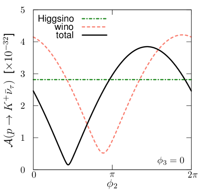
(a) ${\cal A}(p\to K^{+}\overline{\nu}_{\tau})$

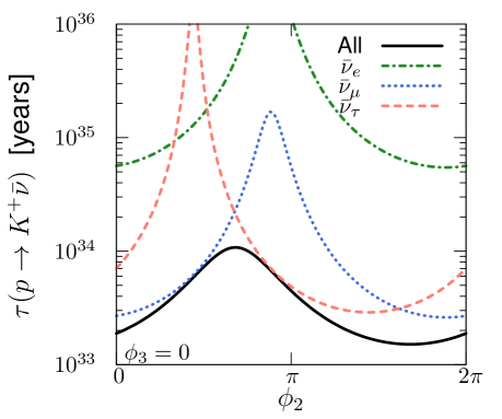
(b) $\tau(p\to K^{+}\overline{\nu}_{i})$

Figure 1: (a): The absolute value of the contributions to the decay amplitude of the $p\to K^{+}\overline{\nu}_{\tau}$ channel as functions of $\phi_{2}$. The red dashed, green dash-dotted and black solid lines represent the absolute values of the wino, Higgsino, and total contributions, respectively. (b): The phase dependences of the lifetimes for the different $p\to K^{+}\overline{\nu}$ decay modes. The green dash-dotted, blue dotted and red dashed lines represent the first-, second-, and third-generation neutrino decay modes, respectively, and the black solid line shows the total lifetime. In both figures, we set $\phi_{3}=0$, and take the parameter point indicated by the star $(\bigstar)$ in Fig. 4.

To show the phase dependence of these contributions more clearly, we show in Fig. 1(a) each contribution to the decay amplitude of the $p\to K^{+}\overline{\nu}_{\tau}$ channel as a function of $\phi_{2}$ with $\phi_{3}$ fixed to be $\phi_{3}=0$. The red dashed, green dash-dotted and black solid lines represent the absolute values of the wino, Higgsino, and total contributions, respectively. We take the parameter point indicated by the star $(\bigstar)$ in Fig. 4 below. This figure shows that the wino contribution can vary by almost an order of magnitude, while the size of the Higgsino contribution remains constant. These contributions are comparable, and thus a significant cancellation can occur. As a result, the total amplitude varies by more than an order of magnitude. The wino contribution is minimized at $\phi_{2}\simeq 0.89\pi$, while the total amplitude is minimized at $\phi_{2}\simeq 0.44\pi$. This mismatch is due to the Higgsino contribution.

In Fig. 1(b) we show the phase dependence of the lifetime of each $p\to K^{+}\overline{\nu}$ decay mode with the same parameter set. The green dash-dotted, blue dotted and red dashed lines represent the first-, second-, and third-generation neutrino decay modes, respectively, while the black solid line shows the total lifetime. We see that the lifetimes of the $\overline{\nu}_{e}$ and $\overline{\nu}_{\mu}$ modes, which are induced by wino exchange only, are maximized at $\phi_{2}\simeq 0.89\pi$, which deviates from the point where $\tau(p\to K^{+}\overline{\nu}_{\tau})$ is maximized. Due to this deviation, the phase dependence of the total lifetime is much smaller than that of each partial lifetime, but still it can change by an ${\cal O}(1)$ factor.

(a) $\tau(p\to K^{+}\overline{\nu})$

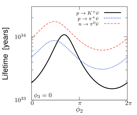
(b) Nucleon decay lifetimes

Figure 2: (a): Contour plot for the proton decay lifetime in units of $10^{35}$ years. The area within the 0.066 contour satisfies the current experimental bound. The peak lifetime is denoted by $\spadesuit$. (b): Lifetimes of the nucleon decay modes as functions of $\phi_{2}$. Calculated for for the reference point indicated by a star $(\bigstar)$ in Fig. 4.

In Fig. 2(a), we show a contour plot for the proton decay lifetime in units of $10^{35}$ years in the $\phi_{2}$–$\phi_{3}$ plane, using the same parameter set as in Fig. 1. We find that the proton lifetime exceeds the current experimental bound, $\tau(p\to K^{+}\overline{\nu})>6.6\times 10^{33}$ yrs [27, 55], in a significant area of the phase space shown by the contour labeled 0.066. The peak lifetime is marked in the upper part of the figure by a spade.

Although the $p\to K^{+}\overline{\nu}$ modes may be suppressed for certain values of the phases, other decay modes that depend on the same phases are not suppressed in the same way. The other decay modes that could restrict the parameter space are $p\to\pi^{+}\overline{\nu}$ and $n\to\pi^{0}\overline{\nu}$. The Wilson coefficients for these proton decay modes are quite similar to those that generate $p\to K^{+}\overline{\nu}$, and depend on exactly the same combination of SUSY parameters. The differences in the calculations of their lifetimes come from their different dependences on CKM matrix elements. The $p\to\pi^{+}\overline{\nu}$ and $n\to\pi^{0}\overline{\nu}$ modes are suppressed relative to the $p\to K^{+}\overline{\nu}$ modes by off-diagonal components of the CKM matrix. Moreover, the experimental constraints on these modes are weaker: $\tau(p\to\pi^{+}\overline{\nu})>3.9\times 10^{32}$ yrs and $n\to\pi^{0}\overline{\nu}>1.1\times 10^{33}$ yrs [27, 56], so these decay modes are less restrictive on the parameter space. To ensure that these modes are not problematic, in Fig. 2(b), we show the lifetimes of these decay modes as functions of $\phi_{2}$ for the same parameter set as in Fig. 1. We find that, although the $p\to\pi^{+}\overline{\nu}$ mode can be dominant, it is still above the present experimental limit. The $n\to\pi^{0}\overline{\nu}$ is always sub-dominant, and again exceeds the current bound. We also note that the $p\to\pi^{+}\overline{\nu}$ and $n\to\pi^{0}\overline{\nu}$ modes exhibit the same phase dependence, since they are related to each other through isospin symmetry.

In the following analysis, we choose the CP-violating phases so as to maximize the $p\to K^{+}\overline{\nu}$ lifetime, thereby obtaining a conservative constraint on the super-GUT model parameter space. Although not shown in the figures below, we have verified that each allowed point also meet the experimental constraint coming from $p\to\pi^{+}\overline{\nu}$ and $n\to\pi^{0}\overline{\nu}$.

4 Results

To appreciate the effect of choosing $M_{in}>M_{GUT}$, we begin by reviewing briefly some results for the CMSSM with $M_{in}=M_{GUT}$. We note that we use here the FeynHiggs 2.11.3 code [57] to compute the Higgs mass. Previously we used FeynHiggs 2.10.0, and we note that due to a bug fix, the new version yields a significant change in $m_{h}$ at large positive $A_{0}$ . A large value of $A_{0}/m_{0}$ is necessary to obtain the correct relic density along the stop-coannihilation strip [59, 14], where the lighter stop and neutralino LSP are nearly degenerate in mass. For $A_{0}/m_{0}\gtrsim 2$, we find that FeynHiggs 2.11.3 results in a $\simeq 1.5$ GeV drop in the value of $m_{h}$ relative to the previous result, necessitating a lower value of $A_{0}/m_{0}$. However, for $A_{0}/m_{0}\lesssim 2$, the stop strip is no longer present. On the other hand, the effect of updating FeynHiggs on $m_{h}$ at large negative $A_{0}/m_{0}$ is less pronounced. We further note that our calculation of the proton lifetime here is also updated with bug-fixes.

4.1 CMSSM update

In view of the proton lifetime constraint, which favours larger sparticle masses, we consider here the possibilities that the correct relic density of neutralino dark matter is obtained either in the focus-point strip [60, 13] or the stop-coannihilation strip [59], updating the results found in [18]. We use SSARD [61] to compute the particle mass spectrum, the dark matter relic density, and proton lifetimes. The discussion of the proton lifetime in Section 3 motivates us to focus on relatively small values of $\tan\beta$. For larger values of $\tan\beta$, the proton lifetime becomes smaller than the current experimental bound, and minimal supersymmetric SU(5) is not viable. For the CMSSM cases with $M_{in}=M_{GUT}$, we have set $c=0$ and taken $M_{H_{C}}$ from Eq. (11).

In Fig. 3, we show four CMSSM $(m_{1/2},m_{0})$ planes displaying the focus-point (left) and stop-coannihilation (right) relic density strips for the two choices of the sign of $\mu$. Higgs mass contours are shown as red dot-dashed curves labeled by $m_{h}$ in GeV in 1 GeV intervals starting at 122 GeV. In the left panels, we choose $A_{0}=0$ with $\mu>0$ (top) and $\mu<0$ (bottom). For this choice of $A_{0}$, there is a relatively minor effect on $m_{h}$ due to the updated version of FeynHiggs. The light mauve shaded region in the parts of the left panels with large $m_{0}/m_{1/2}$ are excluded because there are no solutions to the EWSB conditions: along this boundary $\mu^{2}=0$. Just below the regions where EWSB fails, there are narrow dark blue strips where the relic density falls within the range determined by CMB and other experiments [62] . These strips are in the focus-point region [13, 60]. We note also that the brown shaded regions in the portions of the panels with low $m_{0}/m_{1/2}$ are excluded because there the LSP is the lighter charged stau lepton. The planes also feature stau-coannihilation strips [63] close to the boundaries of these brown shaded regions. They extend to $m_{1/2}\simeq 1$ TeV, but are very difficult to see on the scale of this plot, even with our enhancement of the relic density range. There are also ‘thunderbolt’-shaped brown shaded bands at intermediate $m_{0}/m_{1/2}$ where the chargino is the LSP. There are no accompanying chargino-coannihilation strips, as at these multi-TeV mass scales any such strip would lie within the shaded region and is therefore excluded.

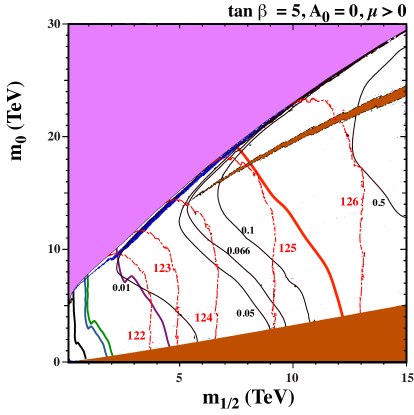
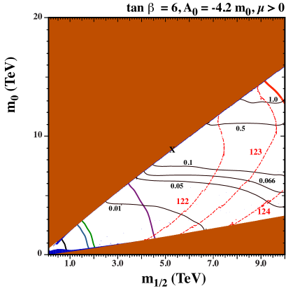
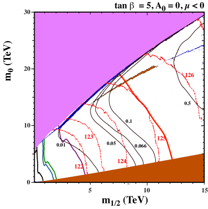
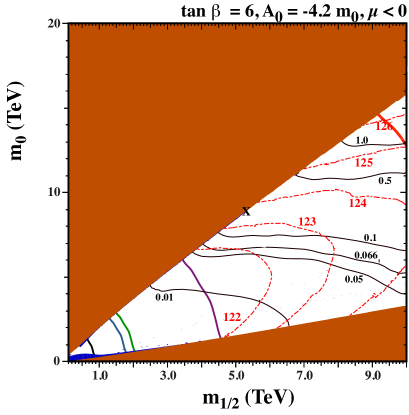
Figure 3: Sample CMSSM $(m_{1/2},m_{0})$ planes showing the focus-point strip for $\tan\beta=5$ and $A_{0}=0$ (left) with $\mu>0$ (upper) and $\mu<0$ (lower), and the stop coannihilation strip with $\tan\beta=6$ and $A_{0}=-4.2\,m_{0}$ (right). In the light mauve shaded regions, it is not possible to satisfy the electroweak symmetry breaking conditions. In the brown shaded regions, the LSP is charged and/or colored. The dark blue shaded strips show the areas where $0.06<\Omega_{\chi}h^{2}<0.2$ in the left panels and the further enlarged range of $0.01<\Omega_{\chi}h^{2}<2.0$ in the right panels. The red dot-dashed contours indicate the Higgs mass, labeled in GeV, and the solid black contours indicate the proton lifetime in units of $10^{35}$ yrs. The bold solid black, blue, green, purple, and red lines in each panel are current and future limits from the LHC at 8 TeV, $300$ and $3000$ fb^-1 at 14 TeV, 3000 fb^-1 with the HE-LHC at 33 TeV, and 3000 fb^-1 with the FCC-hh at 100 TeV, respectively, taken from the analysis of [17].

Contours of the proton lifetime calculated using down-type Yukawa couplings (see the discussion in Section 2.4) are shown as solid black curves that are labeled in units of $10^{35}$ yrs. The current limit $\tau_{p}>6.6\times 10^{33}$ yrs [27, 55] would exclude the entire area below the curve labeled 0.066. For the nominal value of $m_{h}=125$ GeV, neglecting the theoretical uncertainties in the calculation of $m_{h}$, we see that in the upper left plane of Fig. 3 the Higgs contour intersects the focus-point region where $\tau_{p}\approx 5\times 10^{33}$ yrs, very close to the experimental limit. Much of the focus-point strip in this figure may be probed by future proton decay experiments. Changing the sign of $\mu$ has almost no effect on the proton lifetime, as seen in the lower left panel of Fig. 3, but the calculated Higgs mass is smaller by $\sim 1$ GeV, which is less than the uncertainty in the FeynHiggs calculation of $m_{h}$.

In the right panels of Fig. 3, we have chosen large negative $A_{0}/m_{0}=-4.2$ and $\tan\beta=6$, which allows a sufficiently heavy Higgs and a viable stop strip. There are now brown shaded regions in the upper left wedges of the planes where the stop is the LSP (or tachyonic). Though it is barely visible, there is a stop strip that tracks that boundary . Since we have taken an enhanced range for the relic density the blue strip continues to the edge of the plot. In reality, however, the stop strip ends [14] at the position marked by the X in the figure. We see that, for $\mu>0$, the stop strip ends when $m_{h}<122$ GeV, whereas for $\mu<0$ the strip ends when $m_{h}\approx 123.5$ GeV, both of which are acceptable given the uncertainty in the calculation of $m_{h}$. At the endpoint, which occurs at $(m_{1/2},m_{0})\simeq(5.2,8.8)$ TeV, the proton lifetime is approximately $2\times 10^{34}$ yrs. Had we chosen a smaller value of $|A_{0}/m_{0}|$, the stop strip would have extended to higher $m_{h}$. For example, for $\mu<0$, the stop strip extends to 125 GeV for $A_{0}/m_{0}=-3.5$ and the endpoint is found at (5.1,11.3) TeV.

In all of the cases shown in Fig. 3, the favored parameter regions predict the masses of supersymmetric particles to be in the multi-TeV range. For example, as the gluino mass is $\simeq 2\times m_{1/2}$, it is expected to be as large as $\simeq 10$ TeV, which is well above the LHC reach [19, 20]. To see the current and future limits on the CMSSM parameter space from the LHC and future hadron colliders such as the 33 TeV HE-LHC option and the Future Circular Collider (FCC) [64] which aims at 100 TeV proton-proton collisions, we show the limits from LHC at 8 TeV, and sensitivities with $300$ and $3000$ fb^-1 with the LHC at 14 TeV, 3000 fb^-1 with the HE-LHC at 33 TeV, and 3000 fb^-1 with the FCC-hh at 100 TeV as the bold solid black, blue, green, purple, and red lines in each panel in Fig. 3, respectively, following the analysis given in Ref. [17]. As we see, the parameter region in which the proton decay bound is evaded is far beyond the reach of the LHC, but may be probed at the 100 TeV collider. We further note that, while the stop-coannihilation region shown may not be fully probed at 33 TeV, the 100 TeV reach clearly extends beyond the stop endpoint marked by the X. On the other hand, the focus-point region is seen to extend beyond the 100 TeV reach.

4.2 Super-GUT CMSSM

As we discussed earlier, the super-GUT scenario introduces several new parameters, making a complete analysis quite cumbersome. In addition to the CMSSM parameters, we must specify the input universality scale $M_{in}$ and the values of the two GUT couplings $\lambda$ and $\lambda^{\prime}$. In order to understand better the parameter space of the super-GUT models, we begin by considering $(m_{0},A_{0}/m_{0})$ planes for fixed $m_{1/2},\tan\beta,\lambda$, and $\lambda^{\prime}$ and several choices of $M_{in}$, as shown in Fig. 4.

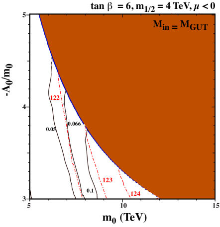
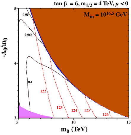
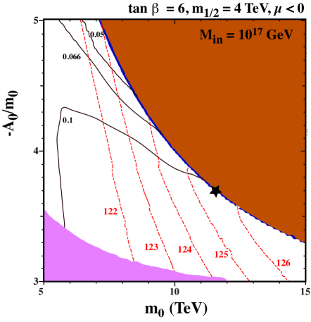
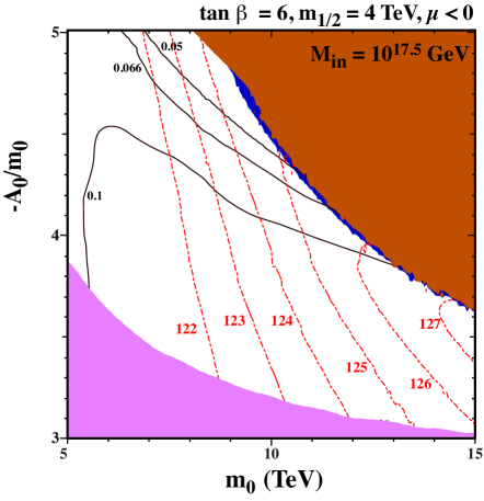
Figure 4: Super-GUT CMSSM $(m_{0},A_{0}/m_{0})$ planes for $\tan\beta=6$ and $\mu<0$. The values of $M_{in}$ are $M_{GUT}$, $10^{16.5}$, $10^{17}$ and $10^{17.5}$ GeV, as indicated. In each panel, we have fixed $m_{1/2}=4$ TeV, $\lambda=0.6$ and $\lambda^{\prime}=0.0001$. In the light mauve shaded regions, it is not possible to satisfy the matching condition for $B$. In the brown shaded regions, the LSP is the stop. The dark blue shaded regions show the areas where $0.01<\Omega_{\chi}h^{2}<2.0$. The red dot-dashed contours indicate the Higgs mass, labeled in GeV, and the solid black contours indicate the proton lifetime in units of $10^{35}$ yrs.

In Fig. 4, we have fixed $\tan\beta=6,m_{1/2}=4$ TeV, $\lambda=0.6$ and $\lambda^{\prime}=10^{-4}$ with $\mu<0$. We have chosen $M_{in}=M_{GUT}$, $10^{16.5}$, $10^{17}$ and $10^{17.5}$ GeV in the upper left, upper right, lower left and lower right panels, respectively. In each panel, the contours for $m_{h}$ and $\tau_{p}$ are drawn using the same line styles as in the previous figure. The brown shaded regions at large $m_{0}$ and $-A_{0}/m_{0}$ are excluded because they contain a stop LSP (or tachyonic stop), and the stop relic density strip tracks this boundary. Because $m_{1/2}$ is fixed, there is no endpoint of the strip within the parameter ranges shown, and the lightest neutralino is an acceptable LSP everywhere along the blue strip (remembering that the thickness of the strip is exaggerated for clarity). For $M_{in}>M_{GUT}$, there is a mauve shaded region at small $m_{0}$ and $-A_{0}/m_{0}$ that grows in size as $M_{in}$ is increased. In this region, the $B$ matching condition (24) is violated, and there is no solution to (28) .

When $M_{in}=M_{GUT}$ with the parameters adopted in Fig. 4, the Higgs mass prefers smaller values of $|A_{0}/m_{0}|$ and larger values of $m_{0}$. In the portion of the strip where $m_{h}>123$ GeV according to FeynHiggs (which is consistent with the experimental measurement), the proton lifetime is $>10^{34}$ yrs. As $M_{in}$ is increased, we see that the stop LSP region moves to larger $m_{0}$ and $|A_{0}/m_{0}|$, while low values of $|A_{0}/m_{0}|$ are excluded because of the $B$ matching condition. For $m_{h}=125$ GeV, the allowed values of $m_{0}$ and $|A_{0}/m_{0}|$ increase as $M_{in}$ is increased. For very large $M_{in}$, we see that the intersection of the $m_{h}$ contour with the stop strip occurs at lower $\tau_{p}$ and for $M_{in}=10^{17.5}$ GeV, the intersection point occurs below the current experimental bound. The star $(\bigstar)$ in the lower left panel with $M_{in}=10^{17}$ GeV, is a benchmark we used in Section 3 to discuss the choice of phases. At this point, which is located at $m_{0}=11.6$ TeV and $A_{0}/m_{0}=-3.7$, we must take $c=-0.0095$ in Eq. (4) in order to obtain $\lambda=0.6$ with $\lambda^{\prime}=10^{-4}$ and we find that the Higgs mass is $m_{h}=125.6$ GeV and $\tau_{p}\approx 10^{34}$ yrs. As shown in Fig. 2(a), this lifetime requires phases $(\phi_{2},\phi_{3})=(0.64,1.96)\pi$. If the phases vanish, the lifetime drops by a factor of about 5 to $\tau_{p}=1.9\times 10^{33}$ yrs. The mass spectrum at this point is shown in Table 1. As can be seen, the gluino mass is $\simeq 2m_{1/2}\simeq 8$ TeV, which is within the reach of the 100 TeV collider [64]. On the other hand, squark masses are $\gtrsim 10$ TeV, and thus it may be difficult to discover squarks even at the 100 TeV collider.

Particle	Mass [TeV]	Particle	Mass [TeV]
${\chi_{1}^{0}}$	1.75	$\chi_{2}^{0}$	3.45
${\chi_{3}^{0}}$	12.8	$\chi_{4}^{0}$	12.8
${\chi^{\pm}_{1}}$	3.45	$\chi_{2}^{\pm}$	12.8
$h$	0.1256	$H$	14.9
$A$	14.9	$\tilde{g}$	7.97
$\tilde{e}_{L}$	11.8	$\tilde{e}_{R}$	12.0
$\tilde{\nu}_{e}$	11.8
$\tilde{\tau}_{1}$	8.29	$\tilde{\tau}_{2}$	11.8
$\tilde{\nu}_{\tau}$	11.8
$\tilde{u}_{L}$	13.2	$\tilde{u}_{R}$	12.9
$\tilde{d}_{L}$	13.2	$\tilde{d}_{R}$	13.0
$\tilde{t}_{1}$	1.76	$\tilde{\tau}_{2}$	7.48
$\tilde{b}_{1}$	7.34	$\tilde{b}_{2}$	12.9

Table 1: Particle Spectrum at the benchmark point indicated by a star $(\bigstar)$ in Fig. 4.

The dependence of these results on $m_{1/2}$ can be gleaned from Fig. 3. For smaller $m_{1/2}$, the Higgs mass and proton lifetime both decrease. At higher $m_{1/2}$, we approach the endpoint of the stop strip. For example, when $m_{1/2}=6$ TeV, there would be no blue strip alongside the red region (which would look similar to the case displayed), as the relic density would exceed the Planck value even for degenerate stops and neutralinos. The results scale as one might expect with $\tan\beta$. At higher $\tan\beta$, the Higgs mass increases while the proton lifetime decreases. For example, at $\tan\beta=7$, for the same value of $A_{0}/m_{0}$, the position of the star when $M_{in}=10^{17}$ GeV moves slightly to $m_{0}=11.5$ TeV, and the Higgs mass increases to 126.1 GeV according to FeynHiggs, but $\tau_{p}$ decreases to $6.2\times 10^{33}$ yrs.

From the discussion in section 3, we expect that there is a strong dependence of $\tau_{p}$ on $\lambda^{\prime}$, while little else is affected. For example, increasing (decreasing) $\lambda^{\prime}$ by an order of magnitude moves the stop-coannihilation strip of the lower left panel of Fig. 4 so that the star would be at 12.1 TeV (11.2 TeV) for $A_{0}/m_{0}$ unchanged. The Higgs mass, $m_{h}$, for this shifted point is almost unchanged, 125.8 GeV (125.5 GeV), while $\tau_{p}$ drops by a factor of 5 (increases by a factor of 4). The dependence on $\lambda$ is discussed in more detail below. We also checked on the effect of changing the sign of $\mu$ and the ratio of $m_{\Sigma}/m_{0}$ for the case considered in the lower left panel of Fig. 4. For both changes, the stop strip and proton lifetime are barely altered. For $\mu>0$, the Higgs mass drops significantly. At the position of the star, the Higgs mass is 117 GeV for $\mu>0$. For this reason we have largely focused on $\mu<0$ in this paper. For $m_{\Sigma}/m_{0}=0.1$ the only noticeable change in the figure is the absence of the $B$ matching constraints which is greatly relaxed when $m_{\Sigma}<m_{0}$. We note that, for $m_{\Sigma}^{2}=0$ or even negative, we are able to recover solutions with $A_{0}=0$. However, when $M_{in}>M_{GUT}$, one does not find a a focus-point region as discussed previously [25].

We next show two examples of $(m_{1/2},m_{0})$ planes for $M_{in}=10^{17}$ GeV, $\tan\beta=6$ and $\mu<0$, which can be compared with the lower right panel of Fig. 3. In the left panel of Fig. 5 we choose $A_{0}/m_{0}=-4.2$ as in Fig. 3. For this value of $M_{in}$, we see the appearance of a mauve shaded region that is excluded because the $B$ matching condition (28) cannot be satisfied. The $X$ located at (5.3, 12.0) TeV again denotes the endpoint of the stop strip. This occurs when $m_{h}=125.5$ GeV and $\tau_{p}=1.1\times 10^{34}$ yrs. Thus only a short segment of the stop strip is viable in this case. In the right panel with $A_{0}/m_{0}=-3.5$, we see that a larger fraction of the plane is excluded by the failure to satisfy the $B$ matching condition. The stop endpoint has moved to higher mass scales $(m_{1/2},m_{0})=(5,16)$ TeV, where $m_{h}=128.1$ GeV and $\tau_{p}=2\times 10^{34}$ yrs, and a larger portion of the strip is viable. In both cases, the viable parameter points can be probed at future collider experiments.

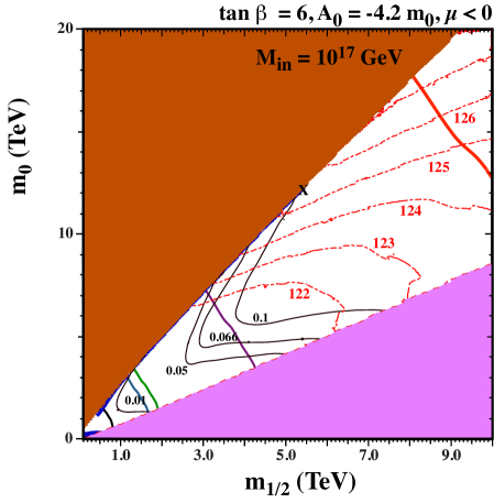
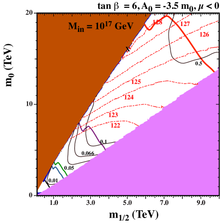
Figure 5: Super-GUT CMSSM $(m_{12},m_{0})$ planes for $M_{in}=10^{17}$ GeV, $\tan\beta=6$ and $\mu<0$, for $A_{0}/m_{0}=-4.2$ (left) and $-3.5$ (right). In each panel, we have fixed $\lambda=0.6$ and $\lambda^{\prime}=0.0001$. Shadings and contours are as in Fig. 3. The mauve shaded regions are excluded because it is not possible to satisfy the matching condition for $B$. The $X$ marks the endpoint of the stop coannihilation strip.

Finally, we discuss the dependence on $\lambda$ and $\lambda^{\prime}$ by considering the $(\lambda,\tan\beta)$ plots shown in Fig. 6, which are for $m_{1/2}=4$ TeV, $m_{0}=10$ TeV and $\mu<0$, with different values of $(M_{in},A_{0}/m_{0},\lambda^{\prime})$. The upper left panel is with the values $(10^{17}$ GeV$,-4.2,0.0001)$, which serve as references. We see that the dark matter strip is adjacent to the brown stop LSP region at $\lambda\simeq 0.67$, growing only slightly with $\tan\beta$ in the range displayed. Along this strip, the proton lifetime constraints is respected for $\tan\beta\lesssim 6.5$, where $m_{h}\sim 125$ GeV according to FeynHiggs. Here, one sees very clearly the dependences of $m_{h}$ and $\tau_{p}$ on $\tan\beta$.

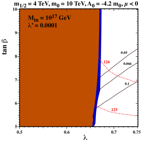
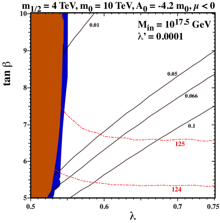
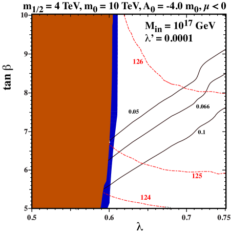
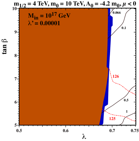
Figure 6: Super-GUT CMSSM $(\lambda,\tan\beta)$ planes with $m_{1/2}=4$ TeV, $m_{0}=10$ TeV, $\mu<0$ and various values of $(M_{in},A_{0}/m_{0},\lambda^{\prime})$ $=(10^{17}$ GeV$,-4.2,0.0001)$ (upper left), $=(10^{17.5}$ GeV$,-4.2,0.0001)$ (upper right), $=(10^{17}$ GeV$,-4.0,0.0001)$ (lower left) and $=(10^{17}$ GeV$,-4.2,0.00001)$ (lower right).

In the upper right panel of Fig. 6, $M_{in}$ is increased to $(10^{17.5})$ GeV, and we see that the dark matter-compatible value of $\lambda$ decreases to $\sim 0.55$ and proton stability then enforces $\tan\beta\lesssim 5.2$, with $m_{h}$ about a GeV smaller than before, but still compatible with the LHC measurement when the FeynHiggs uncertainties are taken into account. Had we decreased $M_{in}$ to $10^{16.5}$ GeV, the coannihilation strip would have moved to $\lambda\approx 0.90$, and the proton stability constraint would have required $\tan\beta\lesssim 8.3$. At the limit, $m_{h}\simeq 127$ GeV and is lower at lower $\tan\beta$.

In the lower left panel of Fig. 6, $-A_{0}/m_{0}$ is decreased to 4.0, with $M_{in}$ and $\lambda^{\prime}$ taking their reference values. In this case, the dark matter constraint requires $\lambda\sim 0.6$ and proton stability then imposes $\tan\beta\lesssim 5.5$, again compatible with $m_{h}$. Increasing $-A_{0}/m_{0}$ to 4.4 would move the coannihilation strip to $\lambda\simeq 0.72$, and the limit on $\tan\beta$ would become $\tan\beta\lesssim 6.6$ with $m_{h}$ close to 126 GeV.

Finally, we see in the lower right panel of Fig. 6 that for $\lambda^{\prime}=0.00001$ and the reference values of $M_{in}$ and $A_{0}/m_{0}$ the dark matter density requires $\lambda\simeq 0.68$ and proton stability then allows $\tan\beta\lesssim 9.8$. Most of this part of the strip is also compatible with $m_{h}$, given the uncertainty in the FeynHiggs calculation. A larger value of $\lambda^{\prime}=0.001$ would require $\tan\beta\lesssim 3.6$, but for this value of $\tan\beta$ the Higgs mass would be unacceptably small, around 120.4 GeV.

5 Discussion

It is frequently stated that the minimal SU(5) GUT model is excluded by the experimental lower limit on the proton lifetime. Taking into account the cosmological constraint on the cold dark matter density, the LHC measurement of $m_{h}$ and the unknown GUT-scale phases appearing in the SU(5) GUT model, we have shown in this paper that this model is quite compatible with the proton stability constraint.

We remind the reader that the amplitudes for the (normally) dominant $p\to K^{+}\overline{\nu}$ decay modes depend on two GUT-scale phases that are beyond the CKM framework, and are not constrained by low-energy physics. As we have discussed in detail, their effects on the $p\to K^{+}\overline{\nu}_{\tau}$ decay amplitude are different from those on the $p\to K^{+}\overline{\nu}_{e,\mu}$ decay amplitudes. We take these effects into account, and also consider their effects on the (normally) subdominant $p\to\pi^{+}\overline{\nu}$ and $n\to\pi^{0}\overline{\nu}$ decays modes. In order to derive the most conservative bounds on the model parameters, we choose the unknown GUT-scale phases so as to maximize the $p\to K^{+}\overline{\nu}$ lifetime.

The compatibility of the supersymmetric GUT model with the proton stability constraint is already visible in the CMSSM with universality of the soft supersymmetry-breaking scalar masses imposed at an input scale $M_{in}=M_{GUT}$ and $\tan\beta\sim 5$. This is visible in Fig. 3 along the upper parts of the focus-point strips in the left panels (with $A_{0}=0$) and of the stop-coannihilation strips in the right panels (with $A_{0}=-4.2m_{0}$). According to the latest version of FeynHiggs, large portions of these strips are also compatible with the experimental measurement of $m_{h}$.

The super-GUT CMSSM with $M_{in}>M_{GUT}$ has more parameters, namely the superpotential couplings $\lambda$ and $\lambda^{\prime}$ as well as $M_{in}$. Correspondingly, the super-GUT CMSSM has greater scope for compatibility with the proton stability and $m_{h}$ constraints. We had previously noted [25] that, for $A_{0}=0$, the focus-point strip move quickly to smaller $m_{1/2}$ and larger $m_{0}$ as $M_{in}$ is increased. The stau LSP region also quickly recedes [24, 25]. Here, we have added the matching condition for $B$, previously neglected in other analyses. This led us to concentrate on relatively large values of $|A_{0}/m_{0}|$. We have given some illustrative examples of suitable parameter choices in Figs. 4, 5 and 6. Typical value of the model parameters are $M_{in}=10^{17}$ GeV, $m_{1/2}=4$ TeV, $m_{0}=10$ TeV, $A_{0}/m_{0}\sim-4$, $\tan\beta\sim 5$, $\lambda\sim 0.6$ and $\lambda^{\prime}\lesssim 0.0001$.

To evade the proton decay constraints, squarks are required to be as heavy as $\gtrsim 10$ TeV, which are hard to probe even at the 100 TeV collider; see [65], however. On the other hand, the gluino mass can be $\lesssim 10$ TeV, which can be probed at the 100 TeV collider [64]. Such heavy sparticle masses require fine-tuning at the electroweak scale [66]; at the expense of this, the simple models discussed in this paper, the minimal SU(5) GUT with (super-GUT) CMSSM, are found to be able to meet all the phenomenological requirements. Of course, by extending the models and/or introducing more complicated mechanisms, we may find a less fine-tuned sparticle spectrum with which the problems in the minimal SU(5), such as the doublet-triplet splitting and the dimension-five proton decay problems, can be evaded—this is beyond the scope of the present work.

In view of the sensitivity of the proton lifetime to the unknown GUT-scale phases, it would interesting to derive model predictions for them—another objective for theories of quark and lepton mixing to bear in mind. Even more interesting would be to devise ways to measure these phases experimentally. In principle, one way to do this would be to measure the ratios of $p\to K^{+}\overline{\nu}$, $p\to\pi^{+}\overline{\nu}$ and $n\to\pi^{0}\overline{\nu}$ decay modes, as illustrated in Fig. 2(b).

This may seem like a distant prospect, but let us remember that the Hyper-Kamiokande project, in particular, has an estimated 90% CL sensitivity to $p\to K^{+}\overline{\nu}$ at the level of $2.5\times 10^{34}$ yrs [67]. This covers the range allowed in Fig. 2 for the reference point indicated by a star $(\bigstar)$ in Fig. 4, and illustrates the capability of Hyper-Kamiokande to probe the GUT-scale physics of proton decay. Let us be optimistic!

Appendix

In this Appendix we review briefly the calculation of nucleon decay rates in the minimal supersymmetric SU(5) GUT. For more details, see Refs. [51, 53, 44, 18].

As mentioned in the text, in the minimal supersymmetric SU(5) GUT model, the dominant contribution to proton decay is induced by the exchange of the color-triplet Higgs multiplets through the Yukawa interactions. We parametrize the SU(5) Yukawa couplings as follows:

$$\left(h_{\bf 10}\right)_{ij}=e^{i\phi_{i}}\delta_{ij}h_{{\bf 10},i}~{},~{}~{}~{}~{}~{}~{}\left(h_{\overline{\bf 5}}\right)_{ij}=V_{ij}^{*}h_{\overline{\bf 5},j}~{}.$$ (A.1)

In this basis, the MSSM matter superfields are embedded as $\Psi_{i}\in\{Q_{i},e^{-i\phi_{i}}\overline{u}_{i},V_{ij}\overline{e}_{j}\}$ and $\Phi_{i}\in\{\overline{d}_{i},L_{i}\}$. Upon integrating out the color-triplet Higgs multiplets, we obtain the dimension-five effective operators in Eq. (34) with the Wilson coefficients in Eq. (36). These coefficients are then evolved down to the SUSY scale $M_{\rm SUSY}$ according to one-loop RGEs, which are presented in Ref. [18].

At $M_{\rm SUSY}$, sfermions in the dimension-five operators are integrated out via the wino- or Higgsino-exchange one-loop diagrams. This gives rise to dimension-six baryon-number-violating operators. Keeping only the dominant contributions, we have

$${\cal L}^{\text{eff}}_{6} =C^{\widetilde{H}}_{i}{\cal O}_{1i33}+C^{\widetilde{W}}_{jk}\widetilde{\cal O}_{1jjk}+C^{\widetilde{W}}_{jk}\widetilde{\cal O}_{j1jk}+\overline{C}^{\widetilde{W}}_{jk}\widetilde{\cal O}_{jj1k}~{},$$ (A.2)

with

$${\cal O}_{ijkl} \equiv\epsilon_{abc}(u^{a}_{Ri}d^{b}_{Rj})(Q_{Lk}^{c}\cdot L_{Ll})~{},$$

$$\widetilde{\cal O}_{ijkl} \equiv\epsilon_{abc}\epsilon^{\alpha\beta}\epsilon^{\gamma\delta}(Q^{a}_{Li\alpha}Q^{b}_{Lj\gamma})(Q_{Lk\delta}^{c}L_{Ll\beta})~{},$$ (A.3)

corresponding to the $O^{(1)}$ and $\widetilde{O}^{(4)}$ in Ref. [68], respectively. Here, $i=1,2$, $j=2,3$, and $k=1,2,3$. The coefficients in Eq. (A.2) are given by

$$C_{i}^{\widetilde{H}}(M_{\text{SUSY}}) =\frac{f_{t}f_{\tau}}{(4\pi)^{2}}C^{*331i}_{5R}(M_{\text{SUSY}})F(\mu,m_{\widetilde{t}_{R}}^{2},m_{\tau_{R}}^{2})~{},$$

$$C^{\widetilde{W}}_{jk}(M_{\text{SUSY}}) =\frac{\alpha_{2}}{4\pi}C^{jj1k}_{5L}(M_{\text{SUSY}})[F(M_{2},m_{\widetilde{Q}_{1}}^{2},m_{\widetilde{Q}_{j}}^{2})+F(M_{2},m_{\widetilde{Q}_{j}}^{2},m_{\widetilde{L}_{k}}^{2})]~{},$$

$$\overline{C}^{\widetilde{W}}_{jk}(M_{\text{SUSY}}) =-\frac{3}{2}\frac{\alpha_{2}}{4\pi}C^{jj1k}_{5L}(M_{\text{SUSY}})[F(M_{2},m_{\widetilde{Q}_{j}}^{2},m_{\widetilde{Q}_{j}}^{2})+F(M_{2},m_{\widetilde{Q}_{1}}^{2},m_{\widetilde{L}_{k}}^{2})]~{},$$ (A.4)

where $m_{\widetilde{Q}_{j}}$ and $m_{\widetilde{L}_{k}}$ are the left-handed squark and left-handed lepton masses, respectively, and 

$$F(M,m_{1}^{2},m_{2}^{2}) \equiv\frac{M}{m_{1}^{2}-m_{2}^{2}}\biggl{[}\frac{m_{1}^{2}}{m_{1}^{2}-M^{2}}\ln\biggl{(}\frac{m_{1}^{2}}{M^{2}}\biggr{)}-\frac{m_{2}^{2}}{m_{2}^{2}-M^{2}}\ln\biggl{(}\frac{m_{2}^{2}}{M^{2}}\biggr{)}\biggr{]}~{}.$$ (A.5)

Note that the wino and Higgsino contributions are proportional to $C_{5L}$ and $C_{5R}$, respectively. The coefficients in Eq. (A.4) are then run down to the electroweak scale by using one-loop RGEs [18, 69].

We consider in this paper the $p\to K^{+}\overline{\nu}$, $p\to\pi^{+}\overline{\nu}$ and $n\to\pi^{0}\overline{\nu}$ channels. Other nucleon decay modes are less important, or their experimental limits are less constraining. The effective interactions for the $p\to K^{+}\overline{\nu}$ is given by

$${\cal L}(p\to K^{+}\bar{\nu}_{i}) =C_{RL}(usd\nu_{i})\bigl{[}\epsilon_{abc}(u_{R}^{a}s_{R}^{b})(d_{L}^{c}\nu_{i})\bigr{]}+C_{RL}(uds\nu_{i})\bigl{[}\epsilon_{abc}(u_{R}^{a}d_{R}^{b})(s_{L}^{c}\nu_{i})\bigr{]}$$

$$+C_{LL}(usd\nu_{i})\bigl{[}\epsilon_{abc}(u_{L}^{a}s_{L}^{b})(d_{L}^{c}\nu_{i})\bigr{]}+C_{LL}(uds\nu_{i})\bigl{[}\epsilon_{abc}(u_{L}^{a}d_{L}^{b})(s_{L}^{c}\nu_{i})\bigr{]}~{},$$ (A.6)

while the $p\to\pi^{+}\overline{\nu}$ and $n\to\pi^{0}\overline{\nu}$ channels are induced by

$${\cal L}(p\to\pi^{+}\bar{\nu}_{i})=C_{RL}(udd\nu_{i})\bigl{[}\epsilon_{abc}(u_{R}^{a}d_{R}^{b})(d_{L}^{c}\nu_{Li})\bigr{]}+C_{LL}(udd\nu_{i})\bigl{[}\epsilon_{abc}(u_{L}^{a}d_{L}^{b})(d_{L}^{c}\nu_{Li})\bigr{]}~{}.$$ (A.7)

These Wilson coefficients are evaluated at the weak scale as follows:

$$C_{RL}(usd\nu_{\tau}) =-V_{td}C^{\widetilde{H}}_{2}(m_{Z})~{},$$

$$C_{RL}(uds\nu_{\tau}) =-V_{ts}C^{\widetilde{H}}_{1}(m_{Z})~{},$$

$$C_{RL}(udd\nu_{\tau}) =-V_{td}C^{\widetilde{H}}_{1}(m_{Z})~{},$$

$$C_{LL}(udd\nu_{k}) =\sum_{j=2,3}V_{j1}V_{j1}C_{jk}^{\widetilde{W}}(m_{Z})~{},$$

$$C_{LL}(usd\nu_{k}) =\sum_{j=2,3}V_{j1}V_{j2}C^{\widetilde{W}}_{jk}(m_{Z})~{},$$

$$C_{LL}(uds\nu_{k}) =\sum_{j=2,3}V_{j1}V_{j2}C^{\widetilde{W}}_{jk}(m_{Z})~{}.$$ (A.8)

We note that the $C_{RL}$ and $C_{LL}$ coefficients are induced by the Higgsino and wino contributions, respectively.

Table 2: Hadron matrix elements for nucleon decay. See Ref. [71] for computations of these values, including error estimates.

Matrix element	Value (GeV2)	Matrix element	Value (GeV2)
$\langle K^{+}|(us)_{L}d_{L}|p\rangle$	0.036	$\langle\pi^{+}|(ud)_{R}d_{L}|p\rangle$	$-0.146$
$\langle K^{+}|(ud)_{L}s_{L}|p\rangle$	0.111	$\langle\pi^{+}|(ud)_{L}d_{L}|p\rangle$	0.188
$\langle K^{+}|(us)_{R}d_{L}|p\rangle$	$-0.054$	$\langle\pi^{0}|(ud)_{R}d_{L}|n\rangle$	$-0.103$
$\langle K^{+}|(ud)_{R}s_{L}|p\rangle$	$-0.093$	$\langle\pi^{0}|(ud)_{L}d_{L}|n\rangle$	0.133

Using the two-loop RGEs given in Ref. [70], we evolve these coefficients down to the hadronic scale $\mu_{\text{had}}=2$ GeV, where the matrix elements of the effective operators are evaluated. Values of the relevant hadron matrix elements are summarized in Table 2, as computed using QCD lattice simulations in Ref. [71]. The decay width of each decay channel is then given by

$$\Gamma(p\to K^{+}\bar{\nu}_{i}) =\frac{m_{p}}{32\pi}\biggl{(}1-\frac{m_{K}^{2}}{m_{p}^{2}}\biggr{)}^{2}|{\cal A}(p\to K^{+}\bar{\nu}_{i})|^{2}~{},$$ (A.9)

$$\Gamma(p\to\pi^{+}\bar{\nu}_{i}) =\frac{m_{p}}{32\pi}\biggl{(}1-\frac{m_{\pi}^{2}}{m_{p}^{2}}\biggr{)}^{2}|{\cal A}(p\to\pi^{+}\bar{\nu}_{i})|^{2}~{},$$ (A.10)

$$\Gamma(n\to\pi^{0}\bar{\nu}_{i}) =\frac{m_{n}}{32\pi}\biggl{(}1-\frac{m_{\pi}^{2}}{m_{n}^{2}}\biggr{)}^{2}|{\cal A}(n\to\pi^{0}\bar{\nu}_{i})|^{2}~{},$$ (A.11)

where $m_{p}$, $m_{n}$, $m_{K}$, and $m_{\pi}$ are the masses of the proton, neutron, kaon, and pion, respectively, and

$${\cal A}(p\to K^{+}\bar{\nu}_{i}) =C_{RL}(usd\nu_{i})\langle K^{+}|(us)_{R}d_{L}|p\rangle+C_{RL}(uds\nu_{i})\langle K^{+}|(ud)_{R}s_{L}|p\rangle$$

$$+C_{LL}(usd\nu_{i})\langle K^{+}|(us)_{L}d_{L}|p\rangle+C_{LL}(uds\nu_{i})\langle K^{+}|(ud)_{L}s_{L}|p\rangle~{},$$

$${\cal A}(p\to\pi^{+}\bar{\nu}_{i}) =C_{RL}(udd\nu_{i})\langle\pi^{+}|(ud)_{R}d_{L}|p\rangle+C_{LL}(udd\nu_{i})\langle\pi^{+}|(ud)_{L}d_{L}|p\rangle~{},$$

$${\cal A}(n\to\pi^{0}\bar{\nu}_{i}) =C_{RL}(udd\nu_{i})\langle\pi^{0}|(ud)_{R}d_{L}|n\rangle+C_{LL}(udd\nu_{i})\langle\pi^{0}|(ud)_{L}d_{L}|n\rangle~{}.$$ (A.12)

We note that the $C_{RL}$ coefficients are non-vanishing only for $i=\tau$. Thus, the decay channels that contain $\overline{\nu}_{e}$ or $\overline{\nu}_{\mu}$ are induced by wino exchange only.

References

- [1] M. Drees and M. M. Nojiri, Phys. Rev. D 47 (1993) 376 [arXiv:hep-ph/9207234]; H. Baer and M. Brhlik, Phys. Rev. D 53 (1996) 597 [arXiv:hep-ph/9508321]; Phys. Rev. D 57 (1998) 567 [arXiv:hep-ph/9706509]; H. Baer, M. Brhlik, M. A. Diaz, J. Ferrandis, P. Mercadante, P. Quintana and X. Tata, Phys. Rev. D 63 (2001) 015007 [arXiv:hep-ph/0005027]; J. R. Ellis, T. Falk, G. Ganis, K. A. Olive and M. Srednicki, Phys. Lett. B 510 (2001) 236 [arXiv:hep-ph/0102098].
- [2] G. L. Kane, C. F. Kolda, L. Roszkowski and J. D. Wells, Phys. Rev. D 49 (1994) 6173 [arXiv:hep-ph/9312272]; J. R. Ellis, T. Falk, K. A. Olive and M. Schmitt, Phys. Lett. B 388 (1996) 97 [arXiv:hep-ph/9607292]; Phys. Lett. B 413 (1997) 355 [arXiv:hep-ph/9705444]; V. D. Barger and C. Kao, Phys. Rev. D 57 (1998) 3131 [arXiv:hep-ph/9704403]; L. Roszkowski, R. Ruiz de Austri and T. Nihei, JHEP 0108 (2001) 024 [arXiv:hep-ph/0106334]; A. Djouadi, M. Drees and J. L. Kneur, JHEP 0108 (2001) 055 [arXiv:hep-ph/0107316]; U. Chattopadhyay, A. Corsetti and P. Nath, Phys. Rev. D 66 (2002) 035003 [arXiv:hep-ph/0201001]; J. R. Ellis, K. A. Olive and Y. Santoso, New Jour. Phys. 4 (2002) 32 [arXiv:hep-ph/0202110]; H. Baer, C. Balazs, A. Belyaev, J. K. Mizukoshi, X. Tata and Y. Wang, JHEP 0207 (2002) 050 [arXiv:hep-ph/0205325]; R. Arnowitt and B. Dutta, arXiv:hep-ph/0211417.
- [3] J. R. Ellis, T. Falk, G. Ganis, K. A. Olive and M. Schmitt, Phys. Rev. D 58 (1998) 095002 [arXiv:hep-ph/9801445]; J. R. Ellis, T. Falk, G. Ganis and K. A. Olive, Phys. Rev. D 62 (2000) 075010 [arXiv:hep-ph/0004169].
- [4] J. R. Ellis, K. A. Olive, Y. Santoso and V. C. Spanos, Phys. Lett. B 565 (2003) 176 [arXiv:hep-ph/0303043]; H. Baer and C. Balazs, JCAP 0305, 006 (2003) [arXiv:hep-ph/0303114]; A. B. Lahanas and D. V. Nanopoulos, Phys. Lett. B 568, 55 (2003) [arXiv:hep-ph/0303130]; U. Chattopadhyay, A. Corsetti and P. Nath, Phys. Rev. D 68, 035005 (2003) [arXiv:hep-ph/0303201]; C. Munoz, Int. J. Mod. Phys. A 19, 3093 (2004) [arXiv:hep-ph/0309346]; R. Arnowitt, B. Dutta and B. Hu, arXiv:hep-ph/0310103; J. Ellis and K. A. Olive, arXiv:1001.3651 [astro-ph.CO], published in Particle dark matter, ed. G. Bertone, pp. 142-163.
- [5] J. Ellis and K. A. Olive, Eur. Phys. J. C 72, 2005 (2012) [arXiv:1202.3262 [hep-ph]].
- [6] O. Buchmueller et al., Eur. Phys. J. C 74 (2014) 3, 2809 [arXiv:1312.5233 [hep-ph]].
- [7] H. Goldberg, Phys. Rev. Lett. 50 (1983) 1419; J. Ellis, J.S. Hagelin, D.V. Nanopoulos, K.A. Olive and M. Srednicki, Nucl. Phys. B238 (1984) 453.
- [8] O. Buchmueller, et al., Eur. Phys. J. C 72 (2012) 2020 [arXiv:1112.3564 [hep-ph]].
- [9] O. Buchmueller, et al., Eur. Phys. J. C 72 (2012) 2243 [arXiv:1207.7315 [hep-ph]].
- [10] O. Buchmueller et al., Eur. Phys. J. C 74 (2014) 6, 2922 [arXiv:1312.5250 [hep-ph]].
- [11] J. Ellis, F. Luo, K. A. Olive and P. Sandick, Eur. Phys. J. C 73, no. 4, 2403 (2013) [arXiv:1212.4476 [hep-ph]].
- [12] H. Baer, V. Barger and A. Mustafayev, Phys. Rev. D 85, 075010 (2012) [arXiv:1112.3017 [hep-ph]]; T. Li, J. A. Maxin, D. V. Nanopoulos and J. W. Walker, Phys. Lett. B 710 (2012) 207 [arXiv:1112.3024 [hep-ph]]; S. Heinemeyer, O. Stal and G. Weiglein, Phys. Lett. B 710, 201 (2012) [arXiv:1112.3026 [hep-ph]]; A. Arbey, M. Battaglia, A. Djouadi, F. Mahmoudi and J. Quevillon, Phys. Lett. B 708 (2012) 162 [arXiv:1112.3028 [hep-ph]]; P. Draper, P. Meade, M. Reece and D. Shih, Phys. Rev. D 85, 095007 (2012) [arXiv:1112.3068 [hep-ph]]; S. Akula, B. Altunkaynak, D. Feldman, P. Nath and G. Peim, Phys. Rev. D 85 (2012) 075001 [arXiv:1112.3645 [hep-ph]]; M. Kadastik, K. Kannike, A. Racioppi and M. Raidal, JHEP 1205 (2012) 061 [arXiv:1112.3647 [hep-ph]]; C. Strege, G. Bertone, D. G. Cerdeno, M. Fornasa, R. Ruiz de Austri and R. Trotta, JCAP 1203, 030 (2012) [arXiv:1112.4192 [hep-ph]]; J. Cao, Z. Heng, D. Li and J. M. Yang, Phys. Lett. B 710 (2012) 665 [arXiv:1112.4391 [hep-ph]]; L. Aparicio, D. G. Cerdeno and L. E. Ibanez, JHEP 1204, 126 (2012) [arXiv:1202.0822 [hep-ph]]; H. Baer, V. Barger and A. Mustafayev, JHEP 1205 (2012) 091 [arXiv:1202.4038 [hep-ph]]; P. Bechtle, T. Bringmann, K. Desch, H. Dreiner, M. Hamer, C. Hensel, M. Kramer and N. Nguyen et al., JHEP 1206, 098 (2012) [arXiv:1204.4199 [hep-ph]]; C. Balazs, A. Buckley, D. Carter, B. Farmer and M. White, arXiv:1205.1568 [hep-ph]; D. Ghosh, M. Guchait, S. Raychaudhuri and D. Sengupta, Phys. Rev. D 86, 055007 (2012) [arXiv:1205.2283 [hep-ph]]; A. Fowlie, M. Kazana, K. Kowalska, S. Munir, L. Roszkowski, E. M. Sessolo, S. Trojanowski and Y. -L. S. Tsai, Phys. Rev. D 86, 075010 (2012) [arXiv:1206.0264 [hep-ph]]; K. Kowalska et al. [BayesFITS Group Collaboration], Phys. Rev. D 87, no. 11, 115010 (2013) [arXiv:1211.1693 [hep-ph]]; C. Strege, G. Bertone, F. Feroz, M. Fornasa, R. Ruiz de Austri and R. Trotta, JCAP 1304, 013 (2013) [arXiv:1212.2636 [hep-ph]]; M. E. Cabrera, J. A. Casas and R. R. de Austri, JHEP 1307 (2013) 182 [arXiv:1212.4821 [hep-ph]]; T. Cohen and J. G. Wacker, JHEP 1309 (2013) 061 [arXiv:1305.2914 [hep-ph]]; S. Henrot-Versillé, Rém. Lafaye, T. Plehn, M. Rauch, D. Zerwas, S. ép. Plaszczynski, B. Rouillé d’Orfeuil and M. Spinelli, Phys. Rev. D 89, 055017 (2014) [arXiv:1309.6958 [hep-ph]]; P. Bechtle, K. Desch, H. K. Dreiner, M. Hamer, M. Kr確er, B. O’Leary, W. Porod and X. Prudent et al., arXiv:1310.3045 [hep-ph]; L. Roszkowski, E. M. Sessolo and A. J. Williams, JHEP 1408, 067 (2014) [arXiv:1405.4289 [hep-ph]]; P. Bechtle et al., Eur. Phys. J. C 76, no. 2, 96 (2016) [arXiv:1508.05951 [hep-ph]].
- [13] J. L. Feng, K. T. Matchev and D. Sanford, Phys. Rev. D 85, 075007 (2012) [arXiv:1112.3021 [hep-ph]]; P. Draper, J. Feng, P. Kant, S. Profumo and D. Sanford, Phys. Rev. D 88, 015025 (2013) [arXiv:1304.1159 [hep-ph]].
- [14] J. Ellis, K. A. Olive and J. Zheng, Eur. Phys. J. C 74, 2947 (2014) [arXiv:1404.5571 [hep-ph]].
- [15] J. Ellis, F. Luo and K. A. Olive, JHEP 1509, 127 (2015) [arXiv:1503.07142 [hep-ph]]; J. Ellis, J. L. Evans, F. Luo and K. A. Olive, JHEP 1602, 071 (2016) [arXiv:1510.03498 [hep-ph]].
- [16] E. A. Bagnaschi et al., Eur. Phys. J. C 75, 500 (2015) [arXiv:1508.01173 [hep-ph]].
- [17] O. Buchmueller, M. Citron, J. Ellis, S. Guha, J. Marrouche, K. A. Olive, K. de Vries and J. Zheng, Eur. Phys. J. C 75, no. 10, 469 (2015) Erratum: [Eur. Phys. J. C 76, no. 4, 190 (2016)] [arXiv:1505.04702 [hep-ph]].
- [18] J. Ellis, J. L. Evans, F. Luo, N. Nagata, K. A. Olive and P. Sandick, Eur. Phys. J. C 76, no. 1, 8 (2016) [arXiv:1509.08838 [hep-ph]].
- [19] G. Aad et al. [ATLAS Collaboration], JHEP 1409 (2014) 176 [arXiv:1405.7875 [hep-ex]]; JHEP 1510, 054 (2015) [arXiv:1507.05525 [hep-ex]]; arXiv:1605.09318 [hep-ex]; The ATLAS collaboration [ATLAS Collaboration], ATLAS-CONF-2016-078; full ATLAS Run I & II results can be found at https://twiki.cern.ch/twiki/bin/view/AtlasPublic/SupersymmetryPublicResults.
- [20] S. Chatrchyan et al. [CMS Collaboration], JHEP 1406 (2014) 055 [arXiv:1402.4770 [hep-ex]]; V. Khachatryan et al. [CMS Collaboration], arXiv:1603.04053 [hep-ex]; CMS Collaboration [CMS Collaboration], CMS-PAS-SUS-16-014; full CMS Run I & II results can be found at http://cms-results.web.cern.ch/cms-results/public-results/publications/SUS/index.html.
- [21] G. Aad et al. [ATLAS Collaboration], Phys. Lett. B 716, 1 (2012) [arXiv:1207.7214 [hep-ex]]; S. Chatrchyan et al. [CMS Collaboration], Phys. Lett. B 716, 30 (2012) [arXiv:1207.7235 [hep-ex]].
- [22] G. Aad et al. [ATLAS and CMS Collaborations], Phys. Rev. Lett. 114 (2015) 191803 [arXiv:1503.07589 [hep-ex]].
- [23] J. R. Ellis, K. A. Olive and P. Sandick, Phys. Lett. B 642, 389 (2006) [hep-ph/0607002]; J. R. Ellis, K. A. Olive and P. Sandick, JHEP 0706, 079 (2007) [arXiv:0704.3446 [hep-ph]]; J. R. Ellis, K. A. Olive and P. Sandick, JHEP 0808, 013 (2008) [arXiv:0801.1651 [hep-ph]].
- [24] L. Calibbi, Y. Mambrini and S. K. Vempati, JHEP 0709, 081 (2007) [arXiv:0704.3518 [hep-ph]]; L. Calibbi, A. Faccia, A. Masiero and S. K. Vempati, Phys. Rev. D 74, 116002 (2006) [arXiv:hep-ph/0605139]; E. Carquin, J. Ellis, M. E. Gomez, S. Lola and J. Rodriguez-Quintero, JHEP 0905 (2009) 026 [arXiv:0812.4243 [hep-ph]].
- [25] J. Ellis, A. Mustafayev and K. A. Olive, Eur. Phys. J. C 69, 201 (2010) [arXiv:1003.3677 [hep-ph]]; J. Ellis, A. Mustafayev and K. A. Olive, Eur. Phys. J. C 69, 219 (2010) [arXiv:1004.5399 [hep-ph]]; J. Ellis, A. Mustafayev and K. A. Olive, Eur. Phys. J. C 71, 1689 (2011) [arXiv:1103.5140 [hep-ph]].
- [26] E. Dudas, Y. Mambrini, A. Mustafayev and K. A. Olive, Eur. Phys. J. C 72, 2138 (2012) [Eur. Phys. J. C 73, 2430 (2013)] [arXiv:1205.5988 [hep-ph]]; E. Dudas, A. Linde, Y. Mambrini, A. Mustafayev and K. A. Olive, Eur. Phys. J. C 73, no. 1, 2268 (2013) [arXiv:1209.0499 [hep-ph]].
- [27] V. Takhistov [Super-Kamiokande Collaboration], arXiv:1605.03235 [hep-ex].
- [28] S. Dimopoulos and H. Georgi, Nucl. Phys. B 193, 150 (1981); N. Sakai, Z. Phys. C 11, 153 (1981).
- [29] T. Goto and T. Nihei, Phys. Rev. D 59, 115009 (1999) [hep-ph/9808255].
- [30] H. Murayama and A. Pierce, Phys. Rev. D 65, 055009 (2002) [hep-ph/0108104].
- [31] H. Georgi and S. L. Glashow, Phys. Rev. Lett. 32, 438 (1974).
- [32] J. R. Ellis and M. K. Gaillard, Phys. Lett. B 88, 315 (1979); C. Panagiotakopoulos and Q. Shafi, Phys. Rev. Lett. 52, 2336 (1984).
- [33] B. Bajc, P. Fileviez Perez and G. Senjanovic, hep-ph/0210374.
- [34] H. Georgi and C. Jarlskog, Phys. Lett. B 86 (1979) 297.
- [35] J. R. Ellis, K. Enqvist, D. V. Nanopoulos and K. Tamvakis, Phys. Lett. B 155, 381 (1985).
- [36] C. T. Hill, Phys. Lett. B 135, 47 (1984); Q. Shafi and C. Wetterich, Phys. Rev. Lett. 52, 875 (1984); M. Drees, Phys. Lett. B 158, 409 (1985); M. Drees, Phys. Rev. D 33, 1468 (1986).
- [37] K. Tobe and J. D. Wells, Phys. Lett. B 588, 99 (2004) [hep-ph/0312159].
- [38] G. Anderson, C. H. Chen, J. F. Gunion, J. D. Lykken, T. Moroi and Y. Yamada, eConf C 960625, SUP107 (1996) [hep-ph/9609457].
- [39] N. Polonsky and A. Pomarol, Phys. Rev. Lett. 73, 2292 (1994) [arXiv:hep-ph/9406224]; Phys. Rev. D 51 (1995) 6532 [arXiv:hep-ph/9410231].
- [40] H. Baer, M. A. Diaz, P. Quintana and X. Tata, JHEP 0004, 016 (2000) [arXiv:hep-ph/0002245].
- [41] J. Hisano, H. Murayama and T. Yanagida, Phys. Rev. Lett. 69, 1014 (1992).
- [42] J. Hisano, H. Murayama and T. Yanagida, Nucl. Phys. B 402, 46 (1993) [hep-ph/9207279].
- [43] J. Hisano, T. Kuwahara and N. Nagata, Phys. Lett. B 723, 324 (2013) [arXiv:1304.0343 [hep-ph]].
- [44] J. L. Evans, N. Nagata and K. A. Olive, Phys. Rev. D 91, 055027 (2015) [arXiv:1502.00034 [hep-ph]].
- [45] L. J. Hall, J. D. Lykken and S. Weinberg, Phys. Rev. D 27, 2359 (1983).
- [46] J. Hisano, H. Murayama and T. Goto, Phys. Rev. D 49, 1446 (1994).
- [47] F. Borzumati and T. Yamashita, Prog. Theor. Phys. 124, 761 (2010) [arXiv:0903.2793 [hep-ph]].
- [48] Y. Kawamura, H. Murayama and M. Yamaguchi, Phys. Rev. D 51, 1337 (1995) [hep-ph/9406245].
- [49] V. D. Barger, M. S. Berger and P. Ohmann, Phys. Rev. D 49 (1994) 4908 [arXiv:hep-ph/9311269]; W. de Boer, R. Ehret and D. I. Kazakov, Z. Phys. C 67 (1995) 647 [arXiv:hep-ph/9405342]; M. Carena, J. R. Ellis, A. Pilaftsis and C. E. Wagner, Nucl. Phys. B 625 (2002) 345 [arXiv:hep-ph/0111245].
- [50] N. Sakai and T. Yanagida, Nucl. Phys. B 197, 533 (1982); S. Weinberg, Phys. Rev. D 26, 287 (1982); J. R. Ellis, D. V. Nanopoulos and S. Rudaz, Nucl. Phys. B 202 (1982) 43.
- [51] J. Hisano, D. Kobayashi, T. Kuwahara and N. Nagata, JHEP 1307, 038 (2013) [arXiv:1304.3651 [hep-ph]].
- [52] D. McKeen, M. Pospelov and A. Ritz, Phys. Rev. D 87, no. 11, 113002 (2013) [arXiv:1303.1172 [hep-ph]]; M. Liu and P. Nath, Phys. Rev. D 87, no. 9, 095012 (2013) [arXiv:1303.7472 [hep-ph]]; M. Dine, P. Draper and W. Shepherd, JHEP 1402, 027 (2014) [arXiv:1308.0274 [hep-ph]]; B. Bajc, S. Lavignac and T. Mede, JHEP 1601, 044 (2016) [arXiv:1509.06680 [hep-ph]].
- [53] N. Nagata and S. Shirai, JHEP 1403, 049 (2014) [arXiv:1312.7854 [hep-ph]].
- [54] J. R. Ellis, M. K. Gaillard and D. V. Nanopoulos, Phys. Lett. B 88, 320 (1979).
- [55] K. Abe et al. [Super-Kamiokande Collaboration], Phys. Rev. D 90, no. 7, 072005 (2014) [arXiv:1408.1195 [hep-ex]].
- [56] K. Abe et al. [Super-Kamiokande Collaboration], Phys. Rev. Lett. 113, no. 12, 121802 (2014) [arXiv:1305.4391 [hep-ex]].
- [57] G. Degrassi, S. Heinemeyer, W. Hollik, P. Slavich and G. Weiglein, Eur. Phys. J. C 28 (2003) 133 [arXiv:hep-ph/0212020]; S. Heinemeyer, W. Hollik and G. Weiglein, Eur. Phys. J. C 9 (1999) 343 [arXiv:hep-ph/9812472]; S. Heinemeyer, W. Hollik and G. Weiglein, Comput. Phys. Commun. 124 (2000) 76 [arXiv:hep-ph/9812320]; M. Frank et al., JHEP 0702 (2007) 047 [arXiv:hep-ph/0611326]; T. Hahn, S. Heinemeyer, W. Hollik, H. Rzehak and G. Weiglein, Phys. Rev. Lett. 112 (2014) 14, 141801 [arXiv:1312.4937 [hep-ph]]; See http://www.feynhiggs.de .
- [58] B. C. Allanach, Comput. Phys. Commun. 143 (2002) 305 [arXiv:hep-ph/0104145].
- [59] C. Boehm, A. Djouadi and M. Drees, Phys. Rev. D 62, 035012 (2000) [arXiv:hep-ph/9911496]; J. R. Ellis, K. A. Olive and Y. Santoso, Astropart. Phys. 18, 395 (2003) [arXiv:hep-ph/0112113]; J. L. Diaz-Cruz, J. R. Ellis, K. A. Olive and Y. Santoso, JHEP 0705, 003 (2007) [arXiv:hep-ph/0701229]; I. Gogoladze, S. Raza and Q. Shafi, Phys. Lett. B 706, 345 (2012) [arXiv:1104.3566 [hep-ph]]; M. A. Ajaib, T. Li and Q. Shafi, Phys. Rev. D 85, 055021 (2012) [arXiv:1111.4467 [hep-ph]].
- [60] J. L. Feng, K. T. Matchev and T. Moroi, Phys. Rev. Lett. 84, 2322 (2000) [arXiv:hep-ph/9908309]; Phys. Rev. D 61, 075005 (2000) [arXiv:hep-ph/9909334]; J. L. Feng, K. T. Matchev and F. Wilczek, Phys. Lett. B 482, 388 (2000) [arXiv:hep-ph/0004043]; H. Baer, T. Krupovnickas, S. Profumo and P. Ullio, JHEP 0510 (2005) 020 [hep-ph/0507282].
- [61] Information about this code is available from K. A. Olive: it contains important contributions from J. Evans, T. Falk, A. Ferstl, G. Ganis, F. Luo, A. Mustafayev, J. McDonald, K. A. Olive, P. Sandick, Y. Santoso, V. Spanos, and M. Srednicki.
- [62] P. A. R. Ade et al. [Planck Collaboration], arXiv:1502.01589 [astro-ph.CO].
- [63] J. Ellis, T. Falk, and K.A. Olive, Phys. Lett. B444 (1998) 367 [arXiv:hep-ph/9810360]; J. Ellis, T. Falk, K.A. Olive, and M. Srednicki, Astr. Part. Phys. 13 (2000) 181 [Erratum-ibid. 15 (2001) 413] [arXiv:hep-ph/9905481]; R. Arnowitt, B. Dutta and Y. Santoso, Nucl. Phys. B 606 (2001) 59 [arXiv:hep-ph/0102181]; M. E. Gómez, G. Lazarides and C. Pallis, Phys. Rev. D D61 (2000) 123512 [arXiv:hep-ph/9907261]; Phys. Lett. B487 (2000) 313 [arXiv:hep-ph/0004028]; Nucl. Phys. B B638 (2002) 165 [arXiv:hep-ph/0203131]; T. Nihei, L. Roszkowski and R. Ruiz de Austri, JHEP 0207 (2002) 024 [arXiv:hep-ph/0206266]; M. Citron, J. Ellis, F. Luo, J. Marrouche, K. A. Olive and K. J. de Vries, Phys. Rev. D 87, 036012 (2013) [arXiv:1212.2886 [hep-ph]].
- [64] T. Golling et al., arXiv:1606.00947 [hep-ph].
- [65] S. A. R. Ellis and B. Zheng, Phys. Rev. D 92 (2015) no.7, 075034 [arXiv:1506.02644 [hep-ph]].
- [66] J. R. Ellis, K. Enqvist, D. V. Nanopoulos and F. Zwirner, Mod. Phys. Lett. A 1 (1986) 57; R. Barbieri and G. F. Giudice, Nucl. Phys. B 306, 63 (1988).
- [67] K. Abe et al., arXiv:1109.3262 [hep-ex].
- [68] L. F. Abbott and M. B. Wise, Phys. Rev. D 22, 2208 (1980).
- [69] R. Alonso, H. M. Chang, E. E. Jenkins, A. V. Manohar and B. Shotwell, Phys. Lett. B 734, 302 (2014) [arXiv:1405.0486 [hep-ph]].
- [70] T. Nihei and J. Arafune, Prog. Theor. Phys. 93, 665 (1995) [hep-ph/9412325].
- [71] Y. Aoki, E. Shintani and A. Soni, Phys. Rev. D 89, no. 1, 014505 (2014) [arXiv:1304.7424 [hep-lat]].