A Short Counterexample Property for Safety and Liveness Verification of Fault-Tolerant Distributed Algorithms

Abstract

Distributed algorithms have many mission-critical applications ranging from embedded systems and replicated databases to cloud computing. Due to asynchronous communication, process faults, or network failures, these algorithms are difficult to design and verify. Many algorithms achieve fault tolerance by using threshold guards that, for instance, ensure that a process waits until it has received an acknowledgment from a majority of its peers. Consequently, domain-specific languages for fault-tolerant distributed systems offer language support for threshold guards.

We introduce an automated method for model checking of safety and liveness of threshold-guarded distributed algorithms in systems where the number of processes and the fraction of faulty processes are parameters. Our method is based on a short counterexample property: if a distributed algorithm violates a temporal specification (in a fragment of LTL), then there is a counterexample whose length is bounded and independent of the parameters. We prove this property by (i) characterizing executions depending on the structure of the temporal formula, and (ii) using commutativity of transitions to accelerate and shorten executions. We extended the ByMC toolset (Byzantine Model Checker) with our technique, and verified liveness and safety of 10 prominent fault-tolerant distributed algorithms, most of which were out of reach for existing techniques.

1 Introduction

Distributed algorithms have many applications in avionic and automotive embedded systems, computer networks, and the internet of things. The central idea is to achieve dependability by replication, and to ensure that all correct replicas behave as one, even if some of the replicas fail. In this way, the correct operation of the system is more reliable than the correct operation of its parts. Fault-tolerant algorithms typically have been used in applications where highest reliability is required because human life is at risk (e.g., automotive or avionic industries), and even unlikely failures of the system are not acceptable. In contrast, in more mainstream applications like replicated databases, human intervention to restart the system from a checkpoint was often considered to be acceptable, so that expensive fault tolerance mechanisms were not used in conventional applications. However, new application domains such as cloud computing provide a new motivation to study fault-tolerant algorithms: with the huge number of computers involved, faults are the norm Netflix [2010] rather than an exception, so that fault tolerance becomes an economic necessity; and so does the correctness of fault tolerance mechanisms. Hence, design, implementation, and verification of distributed systems constitutes an active research area von Gleissenthall et al. [2016]; Killian et al. [2007]; Biely et al. [2013]; Drăgoi et al. [2016]; Lesani et al. [2016]; Peluso et al. [2016]; Konnov et al. [2015]. Although distributed algorithms show complex behavior, and are difficult to understand for human engineers, there is only very limited tool support to catch logical errors in fault-tolerant distributed algorithms at design time.

The state of the art in the design of fault-tolerant systems is exemplified by the recent work on Paxos-like distributed algorithms like Raft Ongaro and Ousterhout [2014] or M²PAXOS Peluso et al. [2016]. The designers encode these algorithms in TLA+ TLA , and use the TLC model checker to automatically find bugs in small instances, i.e., in distributed systems containing, e.g., three processes. Large distributed systems (e.g., clouds) need guarantees for all numbers of processes. These guarantees are typically given using hand-written mathematical proofs. In principle, these proofs could be encoded and machine-checked using the TLAPS proof system Chaudhuri et al. [2010], PVS Lincoln and Rushby [1993], Isabelle Charron-Bost and Merz [2009], Coq Lesani et al. [2016], Nuprl Rahli et al. [2015], or similar systems; but this requires human expertise in the proof checkers and in the application domain, and a lot of effort.

Ensuring correctness of the implementation is an open challenge: As the implementations are done by hand Ongaro and Ousterhout [2014]; Peluso et al. [2016], the connection between the specification and the implementation is informal, such that there is no formal argument about the correctness of the implementation. To address the discrepancy between design, implementation, and verification, Drăgoi et al. Drăgoi et al. [2016] introduced a domain-specific language PSync which is used for two purposes: (i) it compiles into running code, and (ii) it is used for verification. Their verification approach Drăgoi et al. [2014], requires a developer to provide invariants, and similar verification conditions. While this approach requires less human intervention than writing machine-checkable proofs, coming up with invariants of distributed systems requires considerable human ingenuity. The Mace Killian et al. [2007] framework is based on a similar idea, and is an extension to C++. While being fully automatic, their approach to correctness is light-weight in that it uses a tool that explores random walks to find (not necessarily all) bugs, rather than actually verifying systems.

⬇

1case class EchoMsg extends Message

2

3class ReliableBroadcastOnce

4 extends DSLProtocol {

5 val n = ALL.size // nr. processes

6 val t = ALL.size / 3 - 1 // max. faults

7 var accept: Boolean = False

8

9 UPON RECEIVING START WITH v DO {

10 IF v == 1 THEN // check the initial value

11 SEND EchoMsg TO ALL

12 }

13 UPON RECEIVING EchoMsg TIMES t + 1 DO {

14 SEND EchoMsg TO ALL // >= 1 correct

15 }

16 UPON RECEIVING EchoMsg TIMES n - t DO {

17 accept = True // almost all correct

18 }

19}

Figure 1: Code example of a distributed algorithm in DISTAL Biely et al. [2013]. A distributed system consists of $n$ processes, at most $t<n/3$ of which are Byzantine faulty. The correct ones execute the code, and no assumptions is made about the faulty processes.

In this paper we focus on automatic verification methods for programming constructs that are typical for fault-tolerant distributed algorithms. Figure 1 is an example of a distributed algorithm in the domain-specific language DISTAL Biely et al. [2013]. It encodes the core of the reliable broadcast protocol from Srikanth and Toueg [1987], which is used as building block of many fault-tolerant distributed systems. Line 13 and Line 16 use so-called “threshold guards” that check whether a given number of messages from distinct senders arrived at the receiver. As threshold guards are the central algorithmic idea for fault tolerance, domain-specific languages such as DISTAL or PSync have constructs for them (see Drăgoi et al. [2016] for an overview of domain-specific languages and formalization frameworks for distributed systems). For instance, the code in Figure 1 works for systems with $n$ processes among which $t$ can fail, with $t<n/3$ as required for Byzantine fault tolerance Pease et al. [1980]. In such systems, waiting for messages from $n-t$ processes ensures that if all correct processes send messages, then faulty processes cannot prevent progress. Similarly, waiting for $t+1$ messages ensures that at least one message was sent by a correct process. Konnov et al. Konnov et al. [2015] introduced an automatic method to verify safety of algorithms with threshold guards. Their method is parameterized in that it verifies distributed algorithms for all values of parameters ($n$ and $t$) that satisfy a resilience condition ($t<n/3$). This work bares similarities to the classic work on reduction for parallel programs by Lipton Lipton [1975]. Lipton proves statements like “all $P$ operations on a semaphore are left movers with respect to operations on other processes.” He proves that given a run that ends in a given state, the same state is reached by the run in which the $P$ operation has been moved. Konnov et al. Konnov et al. [2015] do a similar analysis for threshold-guarded operations, in which they analyze the relation between statements from Figure 1 like “send EchoMsg” and “UPON RECEIVING EchoMsg TIMES t + 1” in order to determine which statements are movable. From this, they develop an offline partial order reduction that together with acceleration Bardin et al. [2008]; Konnov et al. [2016b] reduced reachability checking to complete bounded model checking using SMT. In this way, they automatically check safety of fault-tolerant algorithms.

However, for fault-tolerant distributed algorithms liveness is as important as safety: This comes from the celebrated impossibility result by Fischer, Lynch, and Paterson Fischer et al. [1985] that states that a fault-tolerant consensus algorithm cannot ensure both safety and liveness in asynchronous systems. It is folklore that designing a safe fault-tolerant distributed algorithm is trivial: just do nothing; e.g., by never committing transactions, one cannot commit them in inconsistent order. Hence, a technique that verifies only safety may establish the “correctness” of a distributed algorithm that never does anything useful. To achieve trust in correctness of a distributed algorithm, we need tools that verify both safety and liveness.

As exemplified by Farzan et al. [2016], liveness verification of parameterized distributed and concurrent systems is still a research challenge. Classic work on parameterized model checking by German and Sistla German and Sistla [1992] has several restrictions on the specifications ($\forall i.\,\phi(i)$) and the computational model (rendezvous), which are incompatible with fault-tolerant distributed algorithms. In fact, none of the approaches (e.g., Clarke et al. [2008]; Emerson and Namjoshi [1995]; Emerson and Kahlon [2003]; Pnueli et al. [2002]) surveyed in Bloem et al. [2015] apply to the algorithms we consider. More generally, in the parameterized case, going from safety to liveness is not straightforward. There are systems where safety is decidable and liveness is not Esparza et al. [1999].

Contributions.

We generalize the approach by Konnov et al. Konnov et al. [2016b, 2015] to liveness by presenting a framework and a model checking tool that takes as input a description of a distributed algorithm (in our variant Gmeiner et al. [2014] of Promela Holzmann [2003]) and specifications in a fragment of linear temporal logic. It then shows correctness for all parameter values (e.g., $n$ and $t$) that satisfy the required resilience condition (e.g., $t<n/3$), or reports a counterexample:

1. As in the classic result by Vardi and Wolper Vardi and Wolper [1986], we observe that it is sufficient to search for counterexamples that have the form of a lasso, i.e., after a finite prefix an infinite loop is entered. Based on this, we analyze specifications automatically, in order to enumerate possible shapes of lassos depending on temporal operators F  and G  and evaluations of threshold guards.

2. We automatically do offline partial order reduction using the algorithm’s description. For this, we introduce a more refined mover analysis for threshold guards and temporal properties. We extend Lipton’s reduction method Lipton [1975] (re-used and extended by many others Cohen and Lamport [1998]; Doeppner [1977]; Lamport and Schneider [1989]; Elmas et al. [2009]; Flanagan et al. [2005]; Konnov et al. [2016b]), so that we maintain invariants, which allows us to go beyond reachability and verify specifications with the temporal operators F  and G .

3. By combining acceleration Bardin et al. [2008]; Konnov et al. [2016b] with Points 1 and 2, we obtain a short counterexample property, that is, that infinite executions (which may potentially be counterexamples) have ”equivalent” representatives of bounded length. The bound depends on the process code and is independent of the parameters. The equivalence is understood in terms of temporal logic specifications that are satisfied by the original executions and the representatives, respectively. We show that the length of the representatives increases mildly compared to reachability checking in Konnov et al. [2015]. This implies a so-called completeness threshold Kroening et al. [2011] for threshold-based algorithms and our fragment of LTL.

4. Consequently, we only have to check a reasonable number of SMT queries that encode parameterized and bounded-length representatives of executions. We show that if the parameterized system violates a temporal property, then SMT reports a counterexample for one of the queries. We prove that otherwise the specification holds for all system sizes.

5. Our theoretical results and our implementation push the boundary of liveness verification for fault-tolerant distributed algorithms. While prior results John et al. [2013] scale just to two out of ten benchmarks from Konnov et al. [2015], we verified safety and liveness of all ten. These benchmarks originate from distributed algorithms Chandra and Toueg [1996]; Srikanth and Toueg [1987]; Bracha and Toueg [1985]; Mostéfaoui et al. [2003]; Raynal [1997]; Guerraoui [2002]; Dobre and Suri [2006]; Brasileiro et al. [2001]; Song and van Renesse [2008] that constitute the core of important services such as replicated state machines.

From a theoretical viewpoint, we introduce new concepts and conduct extensive proofs (the proofs can be found in Konnov et al. [2016a]) for Points 1 and 2. From a practical viewpoint, we have built a complete framework for model checking of fault-tolerant distributed algorithms that use threshold guards, which constitute the central programming paradigm for dependable distributed systems.

2 Representation of Distributed Algorithms

2.1 Threshold Automata

Figure 2: The threshold automaton corresponding to Figure 1 with $\gamma_{1}\colon x\geq(t+1)-f$ and $\gamma_{2}\colon x\geq(n-t)-f$ over parameters $n$, $t$, and $f$, representing the number of processes, the upper bound on the faulty processes (used in the code), and the actual number of faulty processes. The negative number $-f$ in the threshold is used to model the environment, and captures that at most $f$ of the received messages may have been sent by faulty processes.

As internal representation in our tool, and in the theoretical work of this paper, we use threshold automata (TA) defined in Konnov et al. [2016b]. The TA that corresponds to the DISTAL code from Figure 1 is given in Figure 2. The threshold automaton represents the local control flow of a single process, where arrows represent local transitions that are labeled with $\varphi\mapsto\mathsf{act}$: Expression $\varphi$ is a threshold guard and the action $\mathsf{act}$ may increment a shared variable.

Example 2.1.

The TA from Figure 2 is quite similar to the code in Figure 1: if START is called with $v=1$ this corresponds to the initial local state $\ell_{1}$, while otherwise a process starts in $\ell_{0}$. Initially a process has not sent any messages. The local state $\ell_{2}$ in Figure 2 captures that the process has sent EchoMsg and accept evaluates to false, while $\ell_{3}$ captures that the process has sent EchoMsg and accept evaluates to true. The syntax of Figure 1, although checking how many messages of some type are received, hides bookkeeping details and the environment, e.g., message buffers. For our verification technique, we need to make such issues explicit: The shared variable $x$ stores the number of correct processes that have sent EchoMsg. Incrementing $x$ models that EchoMsg is sent when the transition is taken. Then, execution of Line 9 corresponds to the transition $r_{1}$. Executing Line 13 is captured by $r_{2}$: the check whether $t+1$ messages are received is captured by the fact that $r_{2}$ has the guard $\gamma_{1}$, that is, $x\geq(t+1)-f$. Intuitively, this guard checks whether sufficiently many processes have sent EchoMsg (i.e., increased $x$), and takes into account that at most $f$ messages may have been sent by faulty processes. Namely, if we observe the guard in the equivalent form $x+f\geq t+1$, then we notice that it evaluates to true when the total number of received EchoMsg messages from correct processes ($x$) and potentially received messages from faulty processes (at most $f$), is at least $t+1$, which corresponds to the guard of Line 13. Transition $r_{4}$ corresponds to Line 16, $r_{3}$ captures that Line 9 and Line 16 are performed in one protocol step, and $r_{5}$ captures Line 13 and Line 16. $\triangleleft$

While the example shows that the code in a domain-specific language and a TA are quite close, it should be noted that in reality, things are slightly more involved. For instance, the DISTAL runtime takes care of the bookkeeping of sent and received messages (waiting queues at different network layers, buffers, etc.), and just triggers the high-level protocol when a threshold guard evaluates to true. This typically requires counting the number of received messages. While these local counters are present in the implementation, they are abstracted in the TA. For the purpose of this paper we do not need to get into the details. Discussions on data abstraction and automated generation of TAs from code similar to DISTAL can be found in Konnov et al. [2016c].

We recall the necessary definitions introduced in Konnov et al. [2016b]. A threshold automaton is a tuple $\textsf{TA}=({\mathcal{L}},{\mathcal{I}},\Gamma,\Pi,{\mathcal{R}},{\textit{RC\/}\rule{0.0pt}{4.30554pt}})$ whose components are defined as follows: The local states and the initial states are in the finite sets ${\mathcal{L}}$ and ${\mathcal{I}}\subseteq{\mathcal{L}}$, respectively. For simplicity, we identify local states with natural numbers, i.e., ${\mathcal{L}}=\{1,\dots,|{\mathcal{L}}|\}$. Shared variables and parameter variables range over ${\mathbb{N}}_{0}$ and are in the finte sets $\Gamma$ and $\Pi$, respectively. The resilience condition RC is a formula over parameter variables in linear integer arithmetic, and the admissible parameters are $\mathbf{P}_{RC}=\{\mathbf{p}\in{\mathbb{N}}_{0}^{|\Pi|}\colon\mathbf{p}\models{\textit{RC\/}\rule{0.0pt}{4.30554pt}}\}$. After an example for resilience conditions, we will conclude the definition of a threshold automaton by defining ${\mathcal{R}}$ as the finite set of rules.

Example 2.2.

The admissible parameters and resilience conditions are motivated by fault-tolerant distributed algorithms: Let $n$ be the number of processes, $t$ be the assumed number of faulty processes, and in a run, $f$ be the actual number of faults. For these parameters, the famous result by Pease, Shostak and Lamport Pease et al. [1980] states that agreement can be solved iff the resilience condition $n>3t\wedge t\geq f\geq 0$ is satisfied. Given such constraints, the set $\mathbf{P}_{RC}$ is infinite, and in Section 2.2 we will see that this results in an infinite state system. $\triangleleft$

A rule is a tuple $({\mathit{from}},{\mathit{to}},\varphi^{\scriptscriptstyle{\leq}},\varphi^{\scriptscriptstyle{>}},\mathbf{u})$, where ${\mathit{from}}$ and ${\mathit{to}}$ are from ${\mathcal{L}}$, and capture from which local state to which a process moves via that rule. A rule can only be executed if $\varphi^{\scriptscriptstyle{\leq}}$ and $\varphi^{\scriptscriptstyle{>}}$ are true; both are conjunction of guards. Each guard consists of a shared variable $x\in\Gamma$, coefficients $a_{0},\dots,a_{|\Pi|}\in{\mathbb{Z}}$, and parameter variables $p_{1},\dots,p_{|\Pi|}\in\Pi$ so that $x\geq a_{0}+\sum\nolimits_{i=1}^{{|\Pi|}}a_{i}\cdot p_{i}$ is a lower guard and $x<a_{0}+\sum\nolimits_{i=1}^{{|\Pi|}}a_{i}\cdot p_{i}$ is an upper guard. Then, $\Phi^{\mathrm{rise}}$ and $\Phi^{\mathrm{fall}}$ are the sets of lower and upper guards. Rules may increase shared variables using an update vector $\mathbf{u}\in{\mathbb{N}}_{0}^{|\Gamma|}$ that is added to the vector of shared variables. Finally, ${\mathcal{R}}$ is the finite set of rules.

Example 2.3.

A rule corresponds to an edge in Figure 2. The pair $({\mathit{from}},{\mathit{to}})$ encodes the edge while $(\varphi^{\scriptscriptstyle{\leq}},\varphi^{\scriptscriptstyle{>}},\mathbf{u})$ encodes the edge label. For example, rule $r_{2}$ would be $(\ell_{0},\ell_{2},\gamma_{1},\top,1)$. Thus, a rule corresponds to a (guarded) statement from Figure 1 (or combined statements as discussed in Example 2.1). $\triangleleft$

The above definition of TAs is quite general. It allows loops, increase of shared variables in loops, etc. As has been observed in Konnov et al. [2016b], if one does not restrict increases on shared variables, the resulting systems may produce runs that visit infinitely many states, and there is little hope for a complete verification method. Hence, Konnov et al. Konnov et al. [2015] analyzed the TAs of the benchmarks Chandra and Toueg [1996]; Srikanth and Toueg [1987]; Bracha and Toueg [1985]; Mostéfaoui et al. [2003]; Raynal [1997]; Guerraoui [2002]; Dobre and Suri [2006]; Brasileiro et al. [2001]; Song and van Renesse [2008]: They observed that some states have self-loops (corresponding to busy-waiting for messages to arrive) and in the case of failure detector based algorithms Raynal [1997] there are loops that consist of at most two rules. None of the rules in loops increase shared variables. In our theory, we allow more general TAs than actually found in the benchmarks. In more detail, we make the following assumption:

Threshold automata for fault-tolerant distributed algorithms.

As in Konnov et al. [2016b], we assume that if a rule $r$ is in a loop, then $r.\mathbf{u}=\mathbf{0}$. In addition, we use the restriction that all the cycles of a TA are simple, i.e., between any two locations in a cycle there exists exactly one node-disjoint directed path (nodes in cycles may have self-loops). We conjecture that this restriction can be relaxed as in Konnov et al. [2015], but this is orthogonal to our work.

Example 2.4.

In the TA from Figure 2 we use the shared variable $x$ as the number of correct processes that have sent a message. One easily observes that the rules that update $x$ do not belong to loops. Indeed, all the benchmarks Chandra and Toueg [1996]; Srikanth and Toueg [1987]; Bracha and Toueg [1985]; Mostéfaoui et al. [2003]; Raynal [1997]; Guerraoui [2002]; Dobre and Suri [2006]; Brasileiro et al. [2001]; Song and van Renesse [2008] share this structure. This is because at the algorithmic level, all these algorithms are based on the reliable communication assumption (no message loss and no spurious message generation/duplication), and not much is gained by resending the same message. In these algorithms a process checks whether sufficiently many processes (e.g., a majority) have sent a message to signal that they are in some specific local state. Consequently, a receiver would ignore duplicate messages from the same sender. In our analysis we exploit this characteristic of distributed algorithms with threshold guards, and make the corresponding assumption that processes do not send (i.e., increase $x$) from within a loop. Similarly, as a process cannot make the sending of a message undone, we assume that shared variables are never decreased. So, while we need these assumptions to derive our results, they are justified by our application domain. $\triangleleft$

2.2 Counter Systems

A threshold automaton models a single process. Now the question arises how we define the composition of multiple processes that will result in a distributed system. Classically, this is done by parallel composition and interleaving semantics: A state of a distributed system that consists of $n$ processes is modeled as $n$-dimensional vector of local states. The transition to a successor state is then defined by non-deterministically picking a process, say $i$, and changing the $i$th component of the $n$-dimensional vector according to the local transition relation of the process. However, for our domain of threshold-guarded algorithms, we do not care about the precise $n$-dimensional vector so that we use a more efficient encoding: It is well-known that the system state of specific distributed or concurrent systems can be represented as a counter system Lubachevsky [1984]; Pnueli et al. [2002]; Alberti et al. [2016]; Konnov et al. [2016b]: instead of recording for some local state $\ell$, which processes are in $\ell$, we are only interested in how many processes are in $\ell$. In this way, we can efficiently encode transition systems in SMT with linear integer arithmetics. Therefore, we formalize the semantics of the threshold automata by counter systems.

Fix a threshold automaton TA, a function (expressible as linear combination of parameters) $N\colon\mathbf{P}_{RC}\rightarrow{\mathbb{N}}_{0}$ that determines the number of modeled processes, and admissible parameter values $\mathbf{p}\in\mathbf{P}_{RC}$. A counter system $\textsf{Sys}(\textsf{TA})$ is defined as a transition system $(\Sigma,I,R)$, with configurations $\Sigma$ and $I$ and transition relation $R$ defined below.

Definition 2.5.

A configuration $\sigma=({\mathbf{\boldsymbol{\kappa}}},\mathbf{g},\mathbf{p})$ consists of a vector of counter values $\sigma.{\mathbf{\boldsymbol{\kappa}}}\in{\mathbb{N}}_{0}^{|{\mathcal{L}}|}$, a vector of shared variable values $\sigma.\mathbf{g}\in{\mathbb{N}}_{0}^{|\Gamma|}$, and a vector of parameter values $\sigma.\mathbf{p}=\mathbf{p}$. The set $\Sigma$ contains all configurations. The initial configurations are in set $I$, and each initial configuration $\sigma$ satisfies $\sigma.\mathbf{g}=\mathbf{0}$, $\sum_{i\in{\mathcal{I}}}\sigma.{\mathbf{\boldsymbol{\kappa}}}[i]=N(\mathbf{p})$, and $\sum_{i\not\in{\mathcal{I}}}\sigma.{\mathbf{\boldsymbol{\kappa}}}[i]=0$.

Example 2.6.

The safety property from Example 2.2, refers to an initial configuration that satisfies resilience condition $n>3t\wedge t\geq f\geq 0$, e.g., $4>3\cdot 1\wedge 1\geq 0\geq 0$ such that $\sigma.\mathbf{p}=(4,1,0)$. In our encodings we typically have $N$ is the function $(n,t,f)\mapsto n-f$. Further, $\sigma.{\mathbf{\boldsymbol{\kappa}}}[\ell_{0}]=N(\mathbf{p})=n-f=4$ and $\sigma.{\mathbf{\boldsymbol{\kappa}}}[\ell_{i}]=0$, for $\ell_{i}\in{\mathcal{L}}\setminus\{\ell_{0}\}$, and the shared variable $\sigma.\mathbf{g}=0$. $\triangleleft$

A transition is a pair $t=({\mathit{rule}},{\mathit{factor}})$ of a rule and a non-negative integer called the acceleration factor. For $t=({\mathit{rule}},{\mathit{factor}})$ we write $t.\mathbf{u}$ for ${\mathit{rule}}.\mathbf{u}$, etc. A transition $t$ is unlocked in $\sigma$ if $\forall k\in\{0,\dots,t.{\mathit{factor}}-1\}.\;(\sigma.{\mathbf{\boldsymbol{\kappa}}},\sigma.\mathbf{g}+k\cdot t.\mathbf{u},\sigma.\mathbf{p})\models t.\varphi^{\scriptscriptstyle{\leq}}\wedge t.\varphi^{\scriptscriptstyle{>}}.$ A transition $t$ is applicable (or enabled) in $\sigma$, if it is unlocked, and $\sigma.{\mathbf{\boldsymbol{\kappa}}}[t.{\mathit{from}}]\geq t.{\mathit{factor}}$, or $t.{\mathit{factor}}=0$.

Example 2.7.

This notion of applicability contains acceleration and is central for our approach. Intuitively, the value of the factor corresponds to how many times the rule is executed by different processes. In this way, we can subsume steps by an arbitrary number of processes into one transition. Consider Figure 2. If for some $k$, $k$ processes are in location $\ell_{1}$, then in classic modeling it takes $k$ transitions to move these processes one-by-one to $\ell_{2}$. With acceleration, however, these $k$ processes can be moved to $\ell_{2}$ in one step, independently of $k$. In this way, the bounds we compute will be independent of the parameter values. However, assuming $x$ to be a shared variable and $f$ being a parameter that captures the number of faults, our (crash-tolerant) benchmarks include rules like “$x<f\mapsto x\scriptsize{\texttt{++}}$” for local transition to a special “crashed” state. The above definition ensures that at most $f-x$ of these transitions are accelerated into one transition (whose factor thus is at most $f-x$). This precise treatment of threshold guards is crucial for fault-tolerant distributed algorithms. The central contribution of this paper is to show how acceleration can be used to shorten schedules while maintaining specific temporal logic properties. $\triangleleft$

Definition 2.8.

The configuration $\sigma^{\prime}$ is the result of applying the enabled transition $t$ to $\sigma$, if

1. $\sigma^{\prime}.\mathbf{g}=\sigma.\mathbf{g}+t.{\mathit{factor}}\cdot t.\mathbf{u}$

2. $\sigma^{\prime}.\mathbf{p}=\sigma.\mathbf{p}$

3. if $t.{\mathit{from}}\neq t.{\mathit{to}}$ then $\sigma^{\prime}.{\mathbf{\boldsymbol{\kappa}}}[t.{\mathit{from}}]=\sigma.{\mathbf{\boldsymbol{\kappa}}}[t.{\mathit{from}}]-t.{\mathit{factor}}$, $\sigma^{\prime}.{\mathbf{\boldsymbol{\kappa}}}[t.{\mathit{to}}]=\sigma.{\mathbf{\boldsymbol{\kappa}}}[t.{\mathit{to}}]+t.{\mathit{factor}}$, and
   $\forall\ell\in{\mathcal{L}}\setminus\{t.{\mathit{from}},t.{\mathit{to}}\}.\;\sigma^{\prime}.{\mathbf{\boldsymbol{\kappa}}}[\ell]=\sigma.{\mathbf{\boldsymbol{\kappa}}}[\ell]$.

4. if $t.{\mathit{from}}=t.{\mathit{to}}$ then $\sigma^{\prime}.{\mathbf{\boldsymbol{\kappa}}}=\sigma.{\mathbf{\boldsymbol{\kappa}}}.$

In this case we use the notation $\sigma^{\prime}=t(\sigma)$.

Example 2.9.

Let us again consider Figure 2 with $n=4$, $t=1$, and $f=1$. We consider the initial configuration where $\sigma.{\mathbf{\boldsymbol{\kappa}}}[\ell_{1}]=n-f=3$ and $\sigma.{\mathbf{\boldsymbol{\kappa}}}[\ell_{i}]=0$, for $\ell_{i}\in{\mathcal{L}}\setminus\{\ell_{0}\}$. The guard of rule $r_{5}$, $\gamma_{2}\colon x\geq(n-t)-f=2$, initially evaluates to false because $x=0$. The guard of rule $r_{1}$ is true, so that any transition $(r_{1},{\mathit{factor}})$ is unlocked. As $\sigma.{\mathbf{\boldsymbol{\kappa}}}[\ell_{1}]=3$, all transitions $(r_{1},{\mathit{factor}})$, for $0\leq{\mathit{factor}}\leq 3$ are applicable. If the transition $(r_{1},2)$ is applied to the initial configuration, we obtain that $x=2$ so that, after the application, $\gamma_{2}$ evaluates to true. Then $r_{5}$ is unlocked and the transitions $(r_{5},1)$ and $(r_{5},0)$ are applicable as $\sigma.{\mathbf{\boldsymbol{\kappa}}}[\ell_{1}]=1$. Since $\gamma_{2}$ checks for greater or equal, once it becomes true it remains true. Such monotonic behavior is given for all guards, as has already been observed in [Konnov et al., 2016b, Proposition 7], and is a crucial property. $\triangleleft$

The transition relation $R$ is defined as follows: Transition $(\sigma,\sigma^{\prime})$ belongs to $R$ iff there is a rule $r\in{\mathcal{R}}$ and a factor $k\in{\mathbb{N}}_{0}$ such that $\sigma^{\prime}=t(\sigma)$ for $t=(r,k)$. A schedule is a sequence of transitions. For a schedule $\tau$ and an index $i:1\leq i\leq|\tau|$, by $\tau[i]$ we denote the $i$th transition of $\tau$, and by $\tau^{i}$ we denote the prefix $\tau[1],\dots,\tau[i]$ of $\tau$. A schedule $\tau=t_{1},\dots,t_{m}$ is applicable to configuration $\sigma_{0}$, if there is a sequence of configurations $\sigma_{1},\dots,\sigma_{m}$ with $\sigma_{i}=t_{i}(\sigma_{i-1})$ for $1\leq i\leq m$. A schedule $t_{1},\dots,t_{m}$ where $t_{i}.{\mathit{factor}}=1$ for $0<i\leq m$ is called conventional. If there is a $t_{i}.{\mathit{factor}}>1$, then a schedule is accelerated. By $\tau\cdot\tau^{\prime}$ we denote the concatenation of two schedules $\tau$ and $\tau^{\prime}$.

We will reason about schedules in Section 6 for our mover analysis, which is naturally expressed by swapping neighboring transitions in a schedule. To reason about temporal logic properties, we need to reason about the configurations that are “visited” by a schedule. For that we now introduce paths.

A finite or infinite sequence $\sigma_{0},t_{1},\sigma_{1},\dots,t_{k-1},\sigma_{k-1},t_{k},\dots$ of alternating configurations and transitions is called a path, if for every transition $t_{i}$, $i\in{\mathbb{N}}$, in the sequence, holds that $t_{i}$ is enabled in $\sigma_{i-1}$, and $\sigma_{i}=t_{i}(\sigma_{i-1})$. For a configuration $\sigma_{0}$ and a finite schedule $\tau$ applicable to $\sigma_{0}$, by $\textsf{path}(\sigma_{0},\tau)$ we denote $\sigma_{0},t_{1},\sigma_{1},\dots,t_{|\tau|},\sigma_{|\tau|}$ with $\sigma_{i}=t_{i}(\sigma_{i-1})$, for $1\leq i\leq|\tau|$. Similarly, if $\tau$ is an infinite schedule applicable to $\sigma_{0}$, then $\textsf{path}(\sigma_{0},\tau)$ represents an infinite sequence $\sigma_{0},t_{1},\sigma_{1},\dots,t_{k-1},\sigma_{k-1},t_{k},\dots$ where $\sigma_{i}=t_{i}(\sigma_{i-1})$, for all $i>0$.

The evaluation of the threshold guards solely defines whether certain rules are unlocked. As was discussed in Example 2.9, along a path, the evaluations of guards are monotonic. The set of upper guards that evaluate to false and lower guards that evaluate to true — called the context — changes only finitely many times. A schedule can thus be understood as an alternating sequence of schedules without context change, and context-changing transitions. We will recall the definitions of context etc. from Konnov et al. [2015] in Section 5. We say that a schedule $\tau$ is steady for a configuration $\sigma$, if every configuration of $\textsf{path}(\sigma,\tau)$ has the same context.

Due to the resilience conditions and admissible parameters, our counter systems are in general infinite state. The following proposition establishes an important property for verification.

Proposition 2.10.

Every (finite or infinite) path visits finitely many configurations.

Proof.

By Definition 2.8(3), if a transition $t$ is applied to a configuration $\sigma$, then the sum of the counters remains unchanged, that is, $\sum_{\ell\in{\mathcal{L}}}\sigma.{\mathbf{\boldsymbol{\kappa}}}[\ell]=\sum_{\ell\in{\mathcal{L}}}t(\sigma).{\mathbf{\boldsymbol{\kappa}}}[\ell]$. By repeating this argument, the sum of the counters remains stable in a path. By Definition 2.8(2) the parameter values also remain stable in a path.

By Definition 2.8(1), it remains to show that in each path eventually the shared variable $\mathbf{g}$ stop increasing. Let us fix a rule $r=({\mathit{from}},{\mathit{to}},\varphi^{\scriptscriptstyle{\leq}},\varphi^{\scriptscriptstyle{>}},\mathbf{u})$ that increases $\mathbf{g}$. By the definition of a transition, applying some transition $(r,{\mathit{factor}})$ decreases ${\mathbf{\boldsymbol{\kappa}}}[r.{\mathit{from}}]$ by ${\mathit{factor}}$. As by assumption on TAs, $r$ is not in a cycle, ${\mathbf{\boldsymbol{\kappa}}}[r.{\mathit{from}}]$ is increased only finitely often, namely, at most $N(\mathbf{p})$ times. As there are only finitely many rules in a TA, the proposition follows. ∎

3 Verification Problems: Parameterized Reachability vs. Safety & Liveness.

In this section we will discuss the verification problems for fault-tolerant distributed algorithms. A central challenge is to handle resilience conditions precisely.

Example 3.1.

The safety property (unforgeability) of Srikanth and Toueg [1987] expressed in terms of Figure 2 means that no process should ever enter $\ell_{3}$ if initially all processes are in $\ell_{0}$, given that $n>3t\wedge t\geq f\geq 0$. We can express this in the counter system: under the resilience condition $n>3t\wedge t\geq f\geq 0$, given an initial configuration $\sigma$, with $\sigma.{\mathbf{\boldsymbol{\kappa}}}[\ell_{0}]=n-f$, to verify safety, we have to establish the absence of a schedule $\tau$ that satisfies $\sigma^{\prime}=\tau(\sigma)$ and $\sigma^{\prime}.{\mathbf{\boldsymbol{\kappa}}}[\ell_{3}]>0$.

In order to be able to answer this question, we have to deal with these resilience conditions precisely: Observe that $\ell_{3}$ is unreachable, as all outgoing transitions from $\ell_{0}$ contain guards that evaluate to false initially, and since all processes are in $\ell_{0}$ no process ever increases $x$. A slight modification of $t\geq f$ to $t+1\geq f$ in the resilience condition changes the result, i.e., one fault too many breaks the system. For example, if $n=4$, $t=1$, and $f=2$, then the new resilience condition holds, but as the guard $\gamma_{1}:x\geq(t+1)-f$ is now initially true, then one correct process can fire the rule $r_{2}$ and increase $x$. Now when $x=1$, the guard $\gamma_{2}:x\geq(n-t)-f$ becomes true, so that the process can fire the rule $r_{4}$ and reach the state $\ell_{3}$. This tells us that unforgeability is not satisfied in the system where the resilience condition is $n>3t\wedge t+1\geq f\geq 0$. $\triangleleft$

This is the verification question studied in Konnov et al. [2015], which can be formalized as follows:

Definition 3.2 (Parameterized reachability).

Given a threshold automaton TA and a Boolean formula $B$ over $\{{\mathbf{\boldsymbol{\kappa}}}[i]=0\mid i\in{\mathcal{L}}\}$, check whether there are parameter values $\mathbf{p}\in\mathbf{P}_{RC}$, an initial configuration $\sigma_{0}\in I$ with $\sigma_{0}.\mathbf{p}=\mathbf{p}$ and a finite schedule $\tau$ applicable to $\sigma_{0}$ such that $\tau(\sigma_{0})\models B$.

As shown in Konnov et al. [2015], if such a schedule exists, then there is also a schedule of bounded length. In this paper, we do not limit ourselves to reachability, but consider specifications of counterexamples to safety and liveness of FTDAs from the literature. We observe that such specifications use a simple subset of linear temporal logic that contains only the temporal operators F  and G .

Example 3.3.

Consider a liveness property from the distributed algorithms literature called correctness Srikanth and Toueg [1987]:

$$\textsf{{G}}\,\textsf{{F}}\,\psi_{\text{fair}}\rightarrow({\mathbf{\boldsymbol{\kappa}}}[\ell_{0}]=0\rightarrow\textsf{{F}}\,{\mathbf{\boldsymbol{\kappa}}}[\ell_{3}]\neq 0).$$ (1)

Formula $\psi_{\text{fair}}$ expresses the reliable communication assumption of distributed algorithms Fischer et al. [1985]. In this example, $\psi_{\text{fair}}\equiv{\mathbf{\boldsymbol{\kappa}}}[\ell_{1}]=0\wedge(x\geq t+1\rightarrow{\mathbf{\boldsymbol{\kappa}}}[\ell_{0}]=0\wedge{\mathbf{\boldsymbol{\kappa}}}[\ell_{1}]=0)\wedge(x\geq n-t\rightarrow{\mathbf{\boldsymbol{\kappa}}}[\ell_{0}]=0\wedge{\mathbf{\boldsymbol{\kappa}}}[\ell_{2}]=0)$. Intuitively, $\textsf{{G}}\,\textsf{{F}}\,\psi_{\text{fair}}$ means that all processes in $\ell_{1}$ should eventually leave this state, and if sufficiently many messages of type $x$ are sent ($\gamma_{1}$ or $\gamma_{2}$ holds true), then all processes eventually receive them. If they do so, they have to eventually fire rules $r_{1}$, $r_{2}$, $r_{3}$, or $r_{4}$ and thus leave locations $\ell_{0}$, $\ell_{1}$, and $\ell_{2}$. Our approach is based on possible shapes of counterexamples. Therefore, we consider the negation of the specification (1), that is, $\textsf{{G}}\,\textsf{{F}}\,\psi_{\text{fair}}\wedge{\mathbf{\boldsymbol{\kappa}}}[\ell_{0}]=0\wedge\textsf{{G}}\,{\mathbf{\boldsymbol{\kappa}}}[\ell_{3}]=0$. In the following we define the logic that can express such counterexamples. $\triangleleft$

The fragment of LTL limited to F  and G  was studied in Etessami et al. [2002]; Kroening et al. [2011]. We further restrict it to the logic that we call Fault-Tolerant Temporal Logic ($\textsf{ELTL}_{\textsf{FT}}$), whose syntax is shown in Table 1. The formulas derived from cform — called counter formulas — restrict counters, while the formulas derived from gform — called guard formulas — restrict shared variables. The formulas derived from pform are propositional formulas. The temporal operators F  and G  follow the standard semantics Clarke et al. [1999]; Baier and Katoen [2008], that is, for a configuration $\sigma$ and an infinite schedule $\tau$, it holds that  $\textsf{path}(\sigma,\tau)\models\varphi$, if:

1. $\sigma\models\varphi$, when $\varphi$ is a propositional formula,

2. $\exists\tau^{\prime},\tau^{\prime\prime}:\tau=\tau^{\prime}\cdot\tau^{\prime\prime}.\ \textsf{path}(\tau^{\prime}(\sigma),\tau^{\prime\prime})\models\psi$, when $\varphi=\textsf{{F}}\,\psi$,

3. $\forall\tau^{\prime},\tau^{\prime\prime}:\tau=\tau^{\prime}\cdot\tau^{\prime\prime}.\ \textsf{path}(\tau^{\prime}(\sigma),\tau^{\prime\prime})\models\psi$, when $\varphi=\textsf{{G}}\,\psi$.

$$\psi ::=\mathit{pform}\ |\ \textsf{{G}}\,\psi\ |\ \textsf{{F}}\,\psi\ |\ \psi\wedge\psi$$

$$\mathit{pform} ::=\mathit{cform}\ |\ \mathit{gform}\vee\mathit{cform}$$

$$\mathit{cform} ::=\bigvee_{\ell\in\mathit{Locs}}{\mathbf{\boldsymbol{\kappa}}}[\ell]\neq 0\ |\ \bigwedge_{\ell\in\mathit{Locs}}{\mathbf{\boldsymbol{\kappa}}}[\ell]=0\ |\ \mathit{cform}\wedge\mathit{cform}$$

$$\mathit{gform} ::=\mathit{guard}\ |\ \neg\mathit{gform}\ |\ \mathit{gform}\wedge\mathit{gform}$$

Table 1: The syntax of $\textsf{ELTL}_{\textsf{FT}}$-formulas: $\mathit{pform}$ defines propositional formulas, and $\psi$ defines temporal formulas. We assume that $\mathit{Locs}\subseteq{\mathcal{L}}$ and $\mathit{guard}\in\Phi^{\mathrm{rise}}\cup\Phi^{\mathrm{fall}}$.

To stress that the formula should be satisfied by at least one path, we prepend $\textsf{ELTL}_{\textsf{FT}}$-formulas with the existential path quantifier  E . We use the shorthand notation $\mathit{true}$ for a valid propositional formula, e.g., $\bigwedge_{i\in\emptyset}{\mathbf{\boldsymbol{\kappa}}}[i]=0$. We also denote with $\textsf{ELTL}_{\textsf{FT}}$ the set of all formulas that can be written using the logic $\textsf{ELTL}_{\textsf{FT}}$.

We will reason about invariants of the finite subschedules, and consider a propositional formula $\psi$. Given a configuration $\sigma$, a finite schedule $\tau$ applicable to $\sigma$, and $\psi$, by $\textsf{Cfgs}(\sigma,\tau)\models\psi$ we denote that $\psi$ holds in every configuration $\sigma^{\prime}$ visited by the path $\textsf{path}(\sigma,\tau)$. In other words, for every prefix $\tau^{\prime}$ of $\tau$, we have that $\tau^{\prime}(\sigma)\models\psi$.

Definition 3.4 (Parameterized unsafety & non-liveness).

Given a threshold automaton TA and an $\textsf{ELTL}_{\textsf{FT}}{}$ formula $\psi$, check whether there are parameter values $\mathbf{p}\in\mathbf{P}_{RC}$, an initial configuration $\sigma_{0}\in I$ with $\sigma_{0}.\mathbf{p}=\mathbf{p}$, and an infinite schedule $\tau$ of $\textsf{Sys}(\textsf{TA})$ applicable to $\sigma_{0}$ such that $\textsf{path}(\sigma_{0},\tau)\models\psi$.

Complete bounded model checking.

We solve this problem by showing how to reduce it to bounded model checking while guaranteeing completeness. To this end, we have to construct a bounded-length encoding of infinite schedules. In more detail:

• We observe that if $\textsf{path}(\sigma_{0},\tau)\models\psi$, then there is an initial state $\sigma$ and two finite schedules $\vartheta$ and $\rho$ (of unknown length) that can be used to construct an infinite (lasso-shaped) schedule $\vartheta\cdot\rho^{\omega}$, such that $\textsf{path}(\sigma,\vartheta\cdot\rho^{\omega})\models\psi$ (Section 4.1).

• Now given $\vartheta$ and $\rho$, we prove that we can use a $\psi$-specific reduction, to cut $\vartheta$ and $\rho$ into subschedules $\vartheta_{1},\dots,\vartheta_{m}$ and $\rho_{1},\dots,\rho_{n}$, respectively so that the subschedules satisfy subformulas of $\psi$ (Sections 4.2, 4.3 and 5).

• We use an offline partial order reduction, specific to the subformulas of $\psi$, and acceleration to construct representative schedules $\mathsf{rep}[\vartheta_{i}]$ and $\mathsf{rep}[\rho_{j}]$ that satisfy the required $\textsf{ELTL}_{\textsf{FT}}$ formulas that are satisfied $\vartheta_{i}$ and $\rho_{j}$, respectively for $1\leq i\leq m$ and $1\leq j\leq n$. Moreover, $\mathsf{rep}[\vartheta_{i}]$ and $\mathsf{rep}[\rho_{j}]$ are fixed sequences of rules, where bounds on the lengths of the sequences are known (Section 6).

• These fixed sequence of rules can be used to encode a query to the SMT solver (Section 7.1). We ask whether there is an applicable schedule in the counter system that satisfies the sequence of rules and $\psi$ (Section 7.3). If the SMT solver reports a contradiction, there exists no counterexample.

Based on these theoretical results, our tool implements the high-level verification algorithm from Figure 3 (in the comments we give the sections that are concerned with the respective step):

⬇

algorithm parameterized_model_checking(TA, $\varphi$): // see Def. 3.4

${\cal G}$ := cut_graph ($\varphi$) /* Sect. 4 */

${\cal H}$ := threshold_graph(TA) /* Sect. 5 */

for each $\prec$ in topological_orderings(${\cal G}\cup{\cal H}$) do // e.g., using Canfield and Williamson [1995]

check_one_order(TA, $\varphi$, ${\cal G}$, ${\cal H}$, $\prec$) /* Sect. 6-7 */

if SMT_sat() then report the SMT model as a counterexample

Figure 3: A high-level description of the verification algorithm. For details of check_one_order, see Section 7.2 and Figure 10.

4 Shapes of Schedules that Satisfy $\textsf{ELTL}_{\textsf{FT}}$

We characterize all possible shapes of lasso schedules that satisfy an $\textsf{ELTL}_{\textsf{FT}}{}$-formula $\varphi$. These shapes are characterized by so-called cut points: We show that every lasso satisfying $\varphi$ has a fixed number of cut points, one cut point per a subformula of $\varphi$ that starts with F . The configuration in the cut point of a subformula $\textsf{{F}}\,\psi$ must satisfy $\psi$, and all configurations between two cut points must satisfy certain propositional formulas, which are extracted from the subformulas of $\varphi$ that start with G . Our notion of a cut point is motivated by extreme appearances of temporal operators Etessami et al. [2002].

Figure 4: The shapes of lassos that satisfy the formula $\,\textsf{{E}}\,\textsf{{F}}\,(a\wedge\textsf{{F}}\,d\wedge\textsf{{F}}\,e\wedge\textsf{{G}}\,b\wedge\textsf{{G}}\,\textsf{{F}}\,c)$. The crosses show cut points for: (A) formula $\textsf{{F}}\,(a\wedge\textsf{{F}}\,d\wedge\textsf{{F}}\,e\wedge\textsf{{G}}\,b\wedge\textsf{{G}}\,\textsf{{F}}\,c)$, (B) formula $\textsf{{F}}\,d$, (C) formula $\textsf{{F}}\,e$, (D) loop start, (E) formula $\textsf{{F}}\,c$, and (F) loop end.

Example 4.1.

Consider the $\textsf{ELTL}_{\textsf{FT}}$ formula $\varphi\equiv\,\textsf{{E}}\,\textsf{{F}}\,(a\wedge\textsf{{F}}\,d\wedge\textsf{{F}}\,e\wedge\textsf{{G}}\,b\wedge\textsf{{G}}\,\textsf{{F}}\,c)$, where $a,\dots,e$ are propositional formulas, whose structure is not of interest in this section. Formula $\varphi$ is satisfiable by certain paths that have lasso shapes, i.e., a path consists of a finite prefix and a loop, which is repeated infinitely. These lassos may differ in the actual occurrences of the propositions and the start of the loop: For instance, at some point, $a$ holds, and since then $b$ always holds, then $d$ holds at some point, then $e$ holds at some point, then the loop is entered, and $c$ holds infinitely often inside the loop. This is the case (a) shown in Figure 4, where the configurations in the cut points $A$, $B$, $C$, and $D$ must satisfy the propositional formulas $a$, $d$, $e$, and $c$ respectively, and the configurations between $A$ and $F$ must satisfy the propositional formula $b$. This example does not restrict the propositions between the initial state and the cut point A, so that this lasso shape, for instance, also captures the path where $b$ holds from the beginning. There are 20 different lasso shapes for $\varphi$, five of them are shown in the figure. We construct lasso shapes that are sufficient for finding a path satisfying an $\textsf{ELTL}_{\textsf{FT}}$ formula. In this example, it is sufficient to consider lasso shapes (a) and (b), since the other shapes can be constructed from (a) and (b) by unrolling the loop several times. $\triangleleft$

4.1 Restricting Schedules to Lassos

In the seminal paper Vardi and Wolper [1986], Vardi and Wolper showed that if a finite-state transition system $M$ violates an LTL formula — which requires all paths to satisfy the formula — then there is a path in $M$ that (i) violates the formula and (ii) has lasso shape. As our logic $\textsf{ELTL}_{\textsf{FT}}{}$ specifies counterexamples to the properties of fault-tolerant distributed algorithms, we are interested in this result in the following form: if the transition system satisfies an ELTL formula — which requires one path to satisfy the formula — then $M$ has a path that (i) satisfies the formula and (ii) has lasso shape.

As observed above, counter systems are infinite state. Consequently, one cannot apply the results of Vardi and Wolper [1986] directly. However, using Proposition 2.10, we show that a similar result holds for counter systems of threshold automata and $\textsf{ELTL}_{\textsf{FT}}$:

Proposition 4.2.

Given a threshold automaton TA and an $\textsf{ELTL}_{\textsf{FT}}{}$ formula $\varphi$, if $\textsf{Sys}(\textsf{TA})\models\,\textsf{{E}}\,\varphi$, then there are an initial configuration $\sigma_{1}\in I$ and a schedule $\tau\cdot\rho^{\omega}$ with the following properties:

1. the path satisfies the formula: $\textsf{path}(\sigma_{1},\tau\cdot\rho^{\omega})\models\varphi$,

2. application of $\rho$ forms a cycle: $\rho^{k}(\tau(\sigma_{1}))=\tau(\sigma_{1})$ for $k\geq 0$.

Although in Konnov et al. [2016a] we use Büchi automata to prove Proposition 4.2, we do not use Büchi automata in this paper. Since $\textsf{ELTL}_{\textsf{FT}}$ uses only the temporal operators F  and G , we found it much easier to reason about the structure of $\textsf{ELTL}_{\textsf{FT}}{}$ formulas directly (in the spirit of Etessami et al. [2002]) and then apply path reductions, rather than constructing the synchronous product of a Büchi automaton and of a counter system and then finding proper path reductions.

Although Proposition 4.2 guarantees counterexamples of lasso shape, it is not sufficient for model checking: (i) counter systems are infinite state, so that state enumeration may not terminate, and (ii) Proposition 4.2 does not provide us with bounds on the length of the lassos needed for bounded model checking. In the next section, we show how to split a lasso schedule in finite segments and to find constraints on lasso schedules that satisfy an $\textsf{ELTL}_{\textsf{FT}}{}$ formula. In Section 6 we then construct shorter (bounded length) segments.

4.2 Characterizing Shapes of Lasso Schedules

Figure 5: A canonical syntax tree of the $\textsf{ELTL}_{\textsf{FT}}$ formula $\varphi\equiv\textsf{{F}}\,(a\wedge\textsf{{F}}\,d\wedge\textsf{{F}}\,e\wedge\textsf{{G}}\,b\wedge\textsf{{G}}\,\textsf{{F}}\,c)$ considered in Example 4.1. The labels $[w]$ denote identifiers of the tree nodes.

We now construct a cut graph of an $\textsf{ELTL}_{\textsf{FT}}$ formula: Cut graphs constrain the orders in which subformulas that start with the operator F  are witnessed by configurations. The nodes of a cut graph correspond to cut points, while the edges constrain the order between the cut points. Using cut points, we give necessary and sufficient conditions for a lasso to satisfy an $\textsf{ELTL}_{\textsf{FT}}$ formula in Theorems 4.12 and 4.13. Before defining cut graphs, we give the technical definitions of canonical formulas and canonical syntax trees.

Definition 4.3.

We inductively define canonical $\textsf{ELTL}_{\textsf{FT}}$ formulas:

• if $p$ is a propositional formula, then the formula $p\wedge\textsf{{G}}\,\mathit{true}$ is a canonical formula of rank 0,

• if $p$ is a propositional formula and formulas $\psi_{1},\dots,\psi_{k}$ are canonical formulas (of any rank) for some $k\geq 1$, then the formula $p\wedge\textsf{{F}}\,\psi_{1}\wedge\dots\wedge\textsf{{F}}\,\psi_{k}\wedge\textsf{{G}}\,\mathit{true}$ is a canonical formula of rank 1,

• if $p$ is a propositional formula and formulas $\psi_{1},\dots,\psi_{k}$ are canonical formulas (of any rank) for some $k\geq 0$, and $\psi_{k+1}$ is a canonical formula of rank 0 or 1, then the formula $p\wedge\textsf{{F}}\,\psi_{1}\wedge\dots\wedge\textsf{{F}}\,\psi_{k}\wedge\textsf{{G}}\,\psi_{k+1}$ is a canonical formula of rank 2.

Example 4.4.

Let $p$ and $q$ be propositional formulas. The formulas $p\wedge\textsf{{G}}\,\mathit{true}$ and $\mathit{true}\wedge\textsf{{F}}\,(q\wedge\textsf{{G}}\,\mathit{true})\wedge\textsf{{G}}\,(p\wedge\textsf{{G}}\,\mathit{true})$ are canonical, while the formulas $p$, $\textsf{{F}}\,q$, and $\textsf{{G}}\,p$ are not canonical. Continuing Example 4.1, the canonical version of the formula $\textsf{{F}}\,(a\wedge\textsf{{F}}\,d\wedge\textsf{{F}}\,e\wedge\textsf{{G}}\,b\wedge\textsf{{G}}\,\textsf{{F}}\,c)$ is the formula $\textsf{{F}}\,(a\wedge\textsf{{F}}\,(d\wedge\textsf{{G}}\,\mathit{true})\wedge\textsf{{F}}\,(e\wedge\textsf{{G}}\,\mathit{true})\wedge\textsf{{G}}\,(b\wedge\textsf{{F}}\,(c\wedge\textsf{{G}}\,\mathit{true})\wedge\textsf{{G}}\,\mathit{true}))$. $\triangleleft$

We will use formulas in the following canonical form in order to simplify presentation.

Observation 1.

The properties of canonical $\textsf{ELTL}_{\textsf{FT}}$ formulas:

1. Every canonical formula consists of canonical subformulas of the form $p\wedge\textsf{{F}}\,\psi_{1}\wedge\dots\wedge\textsf{{F}}\,\psi_{k}\wedge\textsf{{G}}\,\psi_{k+1}$ for some $k\geq 0$, for a propositional formula $p$, canonical formulas $\psi_{1},\dots,\psi_{k}$, and a formula $\psi_{k+1}$ that is either canonical, or equals to $\mathit{true}$.

2. If a canonical formula contains a subformula $\textsf{{G}}\,(\dots\wedge\textsf{{G}}\,\psi)$, then $\psi$ equals $\mathit{true}$.

Proposition 4.5.

There is a function $\mathit{can}:\textsf{ELTL}_{\textsf{FT}}\rightarrow\textsf{ELTL}_{\textsf{FT}}$ that produces for each formula $\varphi\in\textsf{ELTL}_{\textsf{FT}}$ an equivalent canonical formula $\mathit{can}(\varphi)$.

For an $\textsf{ELTL}_{\textsf{FT}}$ formula, there may be several equivalent canonical formulas, e.g., $p\wedge\textsf{{F}}\,(q\wedge\textsf{{G}}\,\mathit{true})\wedge\textsf{{F}}\,(p\wedge\textsf{{G}}\,\mathit{true})\wedge\textsf{{G}}\,\mathit{true}$ and $p\wedge\textsf{{F}}\,(p\wedge\textsf{{G}}\,\mathit{true})\wedge\textsf{{F}}\,(q\wedge\textsf{{G}}\,\mathit{true})\wedge\textsf{{G}}\,\mathit{true}$ differ in the order of F -subformulas. With the function $\mathit{can}$ we fix one such a formula.

Canonical syntax trees.

The canonical syntax tree of the formula introduced in Example 4.1 is shown in Figure 5. With ${\mathbb{N}}_{0}^{*}$ we denote the set of all finite words over natural numbers — these words are used as node identifiers.

Definition 4.6.

The canonical syntax tree of a formula $\varphi\in\textsf{ELTL}_{\textsf{FT}}$ is the set ${\cal T}(\varphi)\subseteq\textsf{ELTL}_{\textsf{FT}}\times{\mathbb{N}}_{0}^{*}$ constructed inductively as follows:

1. The tree contains the root node labeled with the canonical formula $\mathit{can}(\varphi)$ and id $0$, that is, $\left<\mathit{can}(\varphi),0\right>\in{\cal T}(\varphi)$.

2. Consider a tree node $\left<\psi,w\right>\in{\cal T}(\varphi)$ such that for some canonical formula $\psi^{\prime}\in\textsf{ELTL}_{\textsf{FT}}$ one of the following holds: (a) $\psi=\psi^{\prime}=\mathit{can}(\varphi)$, or (b) $\psi=\textsf{{F}}\,\psi^{\prime}$, or (c) $\psi=\textsf{{G}}\,\psi^{\prime}$.

   If $\psi^{\prime}$ is $p\wedge\textsf{{F}}\,\psi_{1}\wedge\dots\wedge\textsf{{F}}\,\psi_{k}\wedge\textsf{{G}}\,\psi_{k+1}$ for some $k\geq 0$, then the tree ${\cal T}(\varphi)$ contains a child node for each of the conjuncts of $\psi^{\prime}$, that is, $\left<p,w.0\right>\in{\cal T}(\varphi)$, as well as $\left<\textsf{{F}}\,\psi_{i},w.i\right>\in{\cal T}(\varphi)$ and $\left<\textsf{{G}}\,\psi_{j},w.j\right>\in{\cal T}(\varphi)$ for $1\leq i\leq k$ and $j=k+1$.

Observation 2.

The canonical syntax tree ${\cal T}(\varphi)$ of an $\textsf{ELTL}_{\textsf{FT}}$ formula $\varphi$ has the following properties:

• Every node $\left<\psi,w\right>$ has the unique identifier $w$, which encodes the path to the node from the root.

• Every intermediate node is labeled with a temporal operator F  or G  over the conjunction of the formulas in the children nodes.

• The root node is labeled with the formula $\varphi$ itself, and $\varphi$ is equivalent to the conjunction of the root’s children formulas, possibly preceded with a temporal operator F  or G .

The temporal formulas that appear under the operator G  have to be dealt with by the loop part of a lasso. To formalize this, we say that a node with id $w\in{\mathbb{N}}_{0}^{*}$ is covered by a G -node, if $w$ can be split into two words $u_{1},u_{2}\in{\mathbb{N}}_{0}^{*}$ with $w=u_{1}.u_{2}$, and there is a formula $\psi\in\textsf{ELTL}_{\textsf{FT}}$ such that $\left<\textsf{{G}}\,\psi,u_{1}\right>\in{{\cal T}(\varphi)}$.

Figure 6: The cut graph of the canonical syntax tree in Figure 5

Cut graphs.

Using the canonical syntax tree ${\cal T}(\varphi)$ of a formula $\varphi$, we capture in a so-called cut graph the possible orders in which formulas $\textsf{{F}}\,\psi$ should be witnessed by configurations of a lasso-shaped path. We will then use the occurrences of the formula $\psi$ to cut the lasso into bounded finite schedules.

Example 4.7.

Figure 6 shows the cut graph of the canonical syntax tree in Figure 5. It consists of tree node ids for subformulas starting with F , and two special nodes for the start and the end of the loop. In the cut graph, the node with id 0 precedes the node with id 0.1, since at least one configuration satisfying $(a\wedge\textsf{{F}}\,(d\wedge\dots)\wedge\dots)$ should occur on a path before (or at the same moment as) a state satisfying $(d\wedge\dots)$. Similarly, the node with id 0 precedes the node with id 0.2. The nodes with ids 0.1 and 0.2 do not have to precede each other, as the formulas $d$ and $e$ can be satisfied in either order. Since the nodes with the ids $0$, $0.1$, and $0.2$ are not covered by a G -node, they both precede the loop start. The loop start precedes the node with id $0.3.1$, as this node is covered by a G -node. $\triangleleft$

Definition 4.8.

The cut graph ${\cal G}(\varphi)$ of an $\textsf{ELTL}_{\textsf{FT}}$ formula is a directed acyclic graph $({\cal V}_{{\cal G}},{\cal E}_{{\cal G}})$ with the following properties:

1. The set of nodes ${\cal V}_{{\cal G}}=\{\mathsf{loop}_{\mathsf{start}},\mathsf{loop}_{\mathsf{end}}\}\cup\{w\in{\mathbb{N}}_{0}^{*}\mid\exists\psi.\ \left<\textsf{{F}}\,\psi,w\right>\in{\cal T}(\varphi)\}$ contains the tree ids that label F -formulas and two special nodes $\mathsf{loop}_{\mathsf{start}}$ and $\mathsf{loop}_{\mathsf{end}}$, which denote the start and the end of the loop respectively.

2. The set of edges ${\cal E}_{{\cal G}}$ satisfies the following constraints:

   1. Each tree node $\left<\textsf{{F}}\,\psi,w\right>\in{\cal T}(\varphi)$ that is not covered by a G -node precedes the loop start, i.e., $(w,\mathsf{loop}_{\mathsf{start}})\in{\cal E}_{{\cal G}}$.

   2. For each tree node $\left<\textsf{{F}}\,\psi,w\right>\in{\cal T}(\varphi)$ covered by a G -node:

      • the loop start precedes $w$, i.e., $(\mathsf{loop}_{\mathsf{start}},w)\in{\cal E}_{{\cal G}}$, and

      • $w$ precedes the loop end, i.e., $(w,\mathsf{loop}_{\mathsf{end}})\in{\cal E}_{{\cal G}}$.

   3. For each pair of tree nodes $\left<\textsf{{F}}\,\psi_{1},w\right>,\left<\textsf{{F}}\,\psi_{2},w.i\right>\in{\cal T}(\varphi)$ not covered by a G -node, we require $(w,w.i)\in{\cal E}_{{\cal G}}$.

   4. For each pair of tree nodes $\left<\textsf{{F}}\,\psi_{1},w_{1}\right>,\left<\textsf{{F}}\,\psi_{2},w_{2}\right>\in{\cal T}(\varphi)$ that are both covered by a G -node, we require either $(w_{1},w_{2})\in{\cal E}_{{\cal G}}$, or $(w_{2},w_{1})\in{\cal E}_{{\cal G}}$ (but not both).

Definition 4.9.

Given a lasso $\tau\cdot\rho^{\omega}$ and a cut graph ${\cal G}(\varphi)=({\cal V}_{{\cal G}},{\cal E}_{{\cal G}})$, we call a function $\zeta:{\cal V}_{{\cal G}}\to\{0,\dots,|\tau|+|\rho|-1\}$ a cut function, if the following holds:

• $\zeta(\mathsf{loop}_{\mathsf{start}})=|\tau|$ and $\zeta(\mathsf{loop}_{\mathsf{end}})=|\tau|+|\rho|-1$,

• if $(v,v^{\prime})\in{\cal E}_{{\cal G}}$, then $\zeta(v)\leq\zeta(v^{\prime})$.

We call the indices $\{\zeta(v)\mid v\in{\cal V}_{{\cal G}}\}$ the cut points. Given a schedule $\tau$ and an index $k:0\leq k<|\tau|+|\rho|$, we say that the index $k$ cuts $\tau$ into $\pi^{\prime}$ and $\pi^{\prime\prime}$, if $\tau=\pi^{\prime}\cdot\pi^{\prime\prime}$ and $|\pi^{\prime}|=k$.

Informally, for a tree node $\left<\textsf{{F}}\,\psi,w\right>\in{\cal T}(\varphi)$, a cut point $\zeta(w)$ witnesses satisfaction of $\textsf{{F}}\,\psi$, that is, the formula $\psi$ holds at the configuration located at the cut point. It might seem that Definitions 4.8 and 4.9 are too restrictive. For instance, assume that the node $\left<\textsf{{F}}\,\psi,w\right>$ is not covered by a G -node, and there is a lasso schedule $\tau\cdot\rho^{\omega}$ that satisfies the formula $\varphi$ at a configuration $\sigma$. It is possible that the formula $\psi$ is witnessed only by a cut point inside the loop. At the same time, Definition 4.9 forces $\zeta(w)\leq\zeta(\mathsf{loop}_{\mathsf{start}})$. We show that this problem is resolved by unwinding the loop $K$ times for some $K\geq 0$, so that there is a cut function for the lasso with the prefix $\tau\cdot\rho^{K}$ and the loop $\rho$:

Proposition 4.10.

Let $\varphi$ be an $\textsf{ELTL}_{\textsf{FT}}$ formula, $\sigma$ be a configuration and $\tau\cdot\rho^{\omega}$ be a lasso schedule applicable to $\sigma$ such that $\textsf{path}(\sigma,\tau\cdot\rho^{\omega})\models\varphi$ holds. There is a constant $K\geq 0$ and a cut function $\zeta$ such that for every $\left<\textsf{{F}}\,\psi,w\right>\in{\cal G}({\cal T}(\varphi))$ if $\zeta(w)$ cuts $(\tau\cdot\rho^{K})\cdot\rho$ into $\pi^{\prime}$ and $\pi^{\prime\prime}$, then $\psi$ is satisfied at the cut point, that is, $\textsf{path}(\pi^{\prime}(\sigma),\pi^{\prime\prime}\cdot\rho^{\omega})\models\psi$.

Proof sketch.

The detailed proof is given in Konnov et al. [2016a]. We will present the required constant $K\geq 0$ and the cut function $\zeta$. To this end, we use extreme appearances of F -formulas (cf. [Etessami et al., 2002, Sec. 4.3]) and use them to find $\zeta$. An extreme appearance of a formula $\textsf{{F}}\,\psi$ is the furthest point in the lasso that still witnesses $\psi$. There might be a subformula that is required to be witnessed in the prefix, but in $\tau\cdot\rho^{\omega}$it is only witnessed by the loop. To resolve this, we replace $\tau$ by a a longer prefix $\tau\cdot\rho^{K}$, by unrolling the loop $\rho$ several times; more precisely, $K$ times, where $K$ is the number of nodes that should precede the lasso start. In other words, if all extreme appearances of the nodes happen to be in the loop part, and they appear in the order that is against the topological order of the graph ${\cal G}({\cal T}(\varphi))$, we unroll the loop $K$ times (the number of nodes that have to be in the prefix) to find the prefix, in which the nodes respect the topological order of the graph. In the unrolled schedule we can now find extreme appearances of the required subformulas in the prefix. ∎

We show that to satisfy an $\textsf{ELTL}_{\textsf{FT}}$ formula, a lasso should (i) satisfy propositional subformulas of F -formulas in the respective cut points, and (ii) maintain the propositional formulas of G -formulas from some cut point on. This is formalized as a witness.

In the following definition, we use a short-hand notation for propositional subformulas: given an $\textsf{ELTL}_{\textsf{FT}}$-formula $\psi$ and its canonical form $\mathit{can}(\psi)=\psi_{0}\wedge\textsf{{F}}\,\psi_{1}\wedge\dots\wedge\textsf{{F}}\,\psi_{k}\wedge\textsf{{G}}\,\psi_{k+1}$, we use the notation $\mathit{prop}(\psi)$ to denote the formula $\psi_{0}$.

Definition 4.11.

Given a configuration $\sigma$, a lasso $\tau\cdot\rho^{\omega}$ applicable to $\sigma$, and an $\textsf{ELTL}_{\textsf{FT}}$ formula $\varphi$, a cut function $\zeta$ of ${\cal G}({\cal T}(\varphi))$ is a witness of $\textsf{path}(\sigma,\tau\cdot\rho^{\omega})\models\varphi$, if the three conditions hold:

1. For $\mathit{can}(\varphi)\equiv\psi_{0}\wedge\textsf{{F}}\,\psi_{1}\wedge\dots\wedge\textsf{{F}}\,\psi_{k}\wedge\textsf{{G}}\,\psi_{k+1}$:

   1. $\sigma\models\psi_{0}$, and

   2. $\textsf{Cfgs}(\sigma,\tau\cdot\rho)\models\mathit{prop}(\psi_{k+1})$.

2. For $\left<\textsf{{F}}\,\psi,v\right>\in{\cal T}(\varphi)$ with $\zeta(v)<|\tau|$, if $\zeta(v)$ cuts $\tau\cdot\rho$ into $\pi^{\prime}$ and $\pi^{\prime\prime}$ and $\psi\equiv\psi_{0}\wedge\textsf{{F}}\,\psi_{1}\wedge\dots\wedge\textsf{{F}}\,\psi_{k}\wedge\textsf{{G}}\,\psi_{k+1}$, then:

   1. $\pi^{\prime}(\sigma)\models\psi_{0}$, and

   2. $\textsf{Cfgs}(\pi^{\prime}(\sigma),\pi^{\prime\prime})\models\mathit{prop}(\psi_{k+1})$.

3. For $\left<\textsf{{F}}\,\psi,v\right>\in{\cal T}(\varphi)$ with $\zeta(v)\geq|\tau|$, if $\zeta(v)$ cuts $\tau\cdot\rho$ into $\pi^{\prime}$ and $\pi^{\prime\prime}$ and $\psi\equiv\psi_{0}\wedge\textsf{{F}}\,\psi_{1}\wedge\dots\wedge\textsf{{F}}\,\psi_{k}\wedge\textsf{{G}}\,\psi_{k+1}$, then:

   1. $\pi^{\prime}(\sigma)\models\psi_{0}$, and

   2. $\textsf{Cfgs}(\tau(\sigma),\rho)\models\mathit{prop}(\psi_{k+1})$.

Conditions (a) require that propositional formulas hold in a configuration, while conditions (b) require that propositional formulas hold on a finite suffix. Hence, to ensure that a cut function constitutes a witness, one has to check the configurations of a fixed number of finite paths (between the cut points). This property is crucial for the path reduction (see Section 6). Theorems 4.12 and 4.13 show that the existence of a witness is a sound and complete criterion for the existence of a lasso satisfying an $\textsf{ELTL}_{\textsf{FT}}$ formula.

Theorem 4.12 (Soundness).

Let $\sigma$ be a configuration, $\tau\cdot\rho^{\omega}$ be a lasso applicable to $\sigma$, and $\varphi$ be an $\textsf{ELTL}_{\textsf{FT}}$ formula. If there is a witness of $\textsf{path}(\sigma,\tau\cdot\rho^{\omega})\models\varphi$, then the lasso $\tau\cdot\rho^{\omega}$ satisfies $\varphi$, that is $\textsf{path}(\sigma,\tau\cdot\rho^{\omega})\models\varphi$.

Theorem 4.13 (Completeness).

Let $\varphi$ be an $\textsf{ELTL}_{\textsf{FT}}$ formula, $\sigma$ be a configuration and $\tau\cdot\rho^{\omega}$ be a lasso applicable to $\sigma$ such that $\textsf{path}(\sigma,\tau\cdot\rho^{\omega})\models\varphi$ holds. There is a witness of $\textsf{path}(\sigma,(\tau\cdot\rho^{K})\cdot\rho^{\omega})\models\varphi$ for some $K\geq 0$.

Theorem 4.12 is proven for subformulas of $\varphi$ by structural induction on the intermediate nodes of the canonical syntax tree. In the proof of Theorem 4.13 we use Proposition 4.10 to prove the points of Definition 4.11. (The detailed proofs are given in Konnov et al. [2016a].)

4.3 Using Cut Graphs to Enumerate Shapes of Lassos

Proposition 4.2 and Theorem 4.13 suggest that in order to find a schedule that satisfies an $\textsf{ELTL}_{\textsf{FT}}$ formula $\varphi$, it is sufficient to look for lasso schedules that can be cut in such a way that the configurations at the cut points and the configurations between the cut points satisfy certain propositional formulas. In fact, the cut points as defined by cut functions (Definition 4.9) are topological orderings of the cut graph ${\cal G}({\cal T}(\varphi))$. Consequently, by enumerating the topological orderings of the cut graph ${\cal G}({\cal T}(\varphi))$ we can enumerate the lasso shapes, among which there is a lasso schedule satisfying $\varphi$ (if $\varphi$ holds on the counter system). These shapes differ in the order, in which F -subformulas of $\varphi$ are witnessed. For this, one can use fast generation algorithms, e.g., Canfield and Williamson [1995].

Example 4.14.

Consider the cut graph in Figure 6. The ordering of its vertices $0,0.1,0.2,\mathsf{loop}_{\mathsf{start}},0.3.1,\mathsf{loop}_{\mathsf{end}}$ corresponds to the lasso shape (a) shown in Figure 4, while the ordering $\mathsf{loop}_{\mathsf{start}},0,0.2,0.1,\mathsf{loop}_{\mathsf{start}},0.3.1,\mathsf{loop}_{\mathsf{end}}$ corresponds to the lasso shape (b). These are the two lasso shapes that one has to analyze, and they are the result of our construction using the cut graph. The other 18 lasso shapes in the figure are not required, and not constructed by our method. $\triangleleft$

From this observation, we conclude that given a topological ordering $v_{1},\dots,v_{|{\cal V}_{{\cal G}}|}$ of the cut graph ${\cal G}({\cal T}(\varphi))=({\cal V}_{{\cal G}},{\cal E}_{{\cal G}})$, one has to look for a lasso schedule that can be written as an alternating sequence of configurations $\sigma_{i}$ and schedules $\tau_{j}$:

$$\sigma_{0},\tau_{0},\sigma_{1},\tau_{1},\dots,\sigma_{\ell},\tau_{\ell},\dots,\sigma_{|{\cal V}_{{\cal G}}|-1},\tau_{|{\cal V}_{{\cal G}}|},\sigma_{|{\cal V}_{{\cal G}}|},$$ (2)

where $v_{\ell}=\mathsf{loop}_{\mathsf{start}}$, $v_{|{\cal V}_{{\cal G}}|}=\mathsf{loop}_{\mathsf{end}}$, and $\sigma_{\ell}=\sigma_{|{\cal V}_{{\cal G}}|}$. Moreover, by Definition 4.11, the sequence of configurations and schedules should satisfy (C1)–(C3), e.g., if a node $v_{i}$ corresponds to the formula $\textsf{{F}}\,(\psi_{0}\wedge\dots\wedge\textsf{{G}}\,\psi_{k+1})$ and this formula matches Condition (C2), then the following should hold:

1. Configuration $\sigma_{i}$ satisfies the propositional formula: $\sigma_{i}\models\psi_{0}$.

2. All configurations visited by the schedule $\tau_{i}\cdot\dots\cdot\tau_{|{\cal V}_{{\cal G}}|}$ from the configuration $\sigma_{i}$ satisfy the propositional formula $\mathit{prop}(\psi_{k+1})$. Formally, $\textsf{Cfgs}(\sigma_{i},\tau_{i}\cdot\dots\cdot\tau_{|{\cal V}_{{\cal G}}|})\models\mathit{prop}(\psi_{k+1})$.

One can write an SMT query for the sequence (2) satisfying Conditions (C1)–(C3). However, this approach has two problems:

1. The order of rules in schedules $\tau_{0},\dots,\tau_{|{\cal V}_{{\cal G}}|}$ is not fixed. Non-deterministic choice of rules complicates the SMT query.

2. To guarantee completeness of the search, one requires a bound on the length of schedules $\tau_{0},\dots,\tau_{|{\cal V}_{{\cal G}}|}$.

For reachability properties these issues were addressed in Konnov et al. [2015] by showing that one only has to consider specific orders of the rules; so-called representative schedules. To lift this technique to $\textsf{ELTL}_{\textsf{FT}}$, we are left with two issues:

1. The shortening technique applies to steady schedules, i.e., the schedules that do not change evaluation of the guards. Thus, we have to break the schedules $\tau_{0},\dots,\tau_{|{\cal V}_{{\cal G}}|}$ into steady schedules. This issue is addressed in Section 5.

2. The shortening technique preserves state reachability, e.g., after shortening of $\tau_{i}$, the resulting schedule still reaches configuration $\sigma_{i+1}$. But it may violate an invariant such as $\textsf{Cfgs}(\sigma_{i},\tau_{i}\cdot\dots\cdot\tau_{|{\cal V}_{{\cal G}}|})\models\mathit{prop}(\psi_{k+1})$. This issue is addressed in Section 6.

5 Cutting Lassos with Threshold Guards

We introduce threshold graphs to cut a lasso into steady schedules, in order to apply the shortening technique of Section 6. Then, we combine the cut graphs and threshold graphs to cut a lasso into smaller finite segments, which can be first shortened and then checked with the approach introduced in Section 4.3.

Given a configuration $\sigma$, its context $\omega(\sigma)$ is the set that consists of the lower guards unlocked in $\sigma$ and the upper guards locked in $\sigma$, i.e., $\omega(\sigma)=\Omega^{\mathrm{rise}}\cup\Omega^{\mathrm{fall}}$, where $\Omega^{\mathrm{rise}}=\{g\in\Phi^{\mathrm{rise}}\mid\sigma\models g\}$ and $\Omega^{\mathrm{fall}}=\{g\in\Phi^{\mathrm{fall}}\mid\sigma\not\models g\}$. As discussed in Example 2.9 on page 2.9, since the shared variables are never decreased, the contexts in a path are monotonically non-decreasing:

Proposition 5.1 (Prop. 3 of Konnov et al. [2015]).

If a transition $t$ is enabled in a configuration $\sigma$, then $\omega(\sigma)\subseteq\omega(t(\sigma))$.

Example 5.2.

Continuing Example 2.9, which considers the TA in Figure 2. Both threshold guards $\gamma_{1}$ and $\gamma_{2}$ are false in the initial state $\sigma$. Thus, $\omega(\sigma)=\emptyset$. The transition $t=(r_{1},1)$ unlocks the guard $\gamma_{1}$, i.e., $\omega(t(\sigma))=\{\gamma_{1}\}$. $\triangleleft$

As the transitions of the counter system $\textsf{Sys}(\textsf{TA})$ never decrease shared variables, the loop of a lasso schedule must be steady:

Proposition 5.3.

For each configuration $\sigma$ and a schedule $\tau\cdot\rho^{\omega}$, if $\rho^{k}(\tau(\sigma))=\tau(\sigma)$ for $k\geq 0$, then the loop $\rho$ is steady for $\tau(\sigma)$, that is, $\omega(\rho(\tau(\sigma)))=\omega(\tau(\sigma))$.

In Konnov et al. [2015], Proposition 5.1 was used to cut a finite path into segments, one per context. We introduce threshold graphs and their topological orderings to apply this idea to lasso schedules.

Definition 5.4.

A threshold graph is ${\cal H}(\textsf{TA})=({\cal V}_{{\cal H}},{\cal E}_{{\cal H}})$ such that:

• The vertices set ${\cal V}_{{\cal H}}$ contains the threshold guards and the special node $\mathsf{loop}_{\mathsf{start}}$, i.e., ${\cal V}_{{\cal H}}=\Phi^{\mathrm{rise}}\cup\Phi^{\mathrm{fall}}\cup\{\mathsf{loop}_{\mathsf{start}}\}$.

• There is an edge from a guard $g_{1}\in\Phi^{\mathrm{rise}}$ to a guard $g_{2}\in\Phi^{\mathrm{rise}}$, if $g_{2}$ cannot be unlocked before $g_{1}$, i.e., $(g_{1},g_{2})\in{\cal E}_{{\cal H}}$, if for each configuration $\sigma\in\Sigma$, $\sigma\models g_{2}$ implies $\sigma\models g_{1}$.

• There is an edge from a guard $g_{1}\in\Phi^{\mathrm{fall}}$ to a guard $g_{2}\in\Phi^{\mathrm{fall}}$, if $g_{2}$ cannot be locked before $g_{1}$, i.e., $(g_{1},g_{2})\in{\cal E}_{{\cal H}}$, if for each configuration $\sigma\in\Sigma$, $\sigma\not\models g_{2}$ implies $\sigma\not\models g_{1}$.

Note that the conditions in Definition 5.4 can be easily checked with an SMT solver, for all configurations.

Example 5.5.

The threshold graph of the TA in Figure 2 has the vertices ${\cal V}_{{\cal H}}=\{\gamma_{1},\gamma_{2},\mathsf{loop}_{\mathsf{start}}\}$ and the edges ${\cal E}_{{\cal H}}=\{(\gamma_{1},\gamma_{2})\}$. $\triangleleft$

Figure 7: The shapes of lassos to check the correctness property in Example 3.3. Recall that $\gamma_{1}$ and $\gamma_{2}$ are the threshold guards, defined as $x\geq t+1-f$ and $x\geq n-t-f$ respectively.

Similar to Section 4.3, we consider a topological ordering $g_{1},\dots,g_{\ell},\dots,g_{|{\cal V}_{{\cal H}}|}$ of the vertices of the threshold graph. The node $g_{\ell}=\mathsf{loop}_{\mathsf{start}}$ indicates the point where a loop should start, and thus by Proposition 5.3, after that point the context does not change. Thus, we consider only the subsequence $g_{1},\dots,g_{\ell-1}$ and split the path $\textsf{path}(\sigma,\tau\cdot\rho)$ of a lasso schedule $\tau\cdot\rho^{\omega}$ into an alternating sequence of configurations $\sigma_{i}$ and schedules $\tau_{0}$ and $t_{j}\cdot\tau_{j}$, for $1\leq j<\ell$, ending up with the loop $\rho$ (starting in $\sigma_{\ell-1}$ and ending in $\sigma_{\ell}=\sigma_{\ell-1}$):

$$\sigma_{0},\tau_{0},\sigma_{1},(t_{1}\cdot\tau_{1}),\dots,\sigma_{\ell-2},(t_{\ell-1}\cdot\tau_{\ell-1}),\sigma_{\ell-1},\rho,\sigma_{\ell}$$ (3)

In this sequence, the transitions $t_{1},\dots,t_{\ell-1}$ change the context, and the schedules $\tau_{0},\tau_{1},\dots,\tau_{\ell-1},\rho$ are steady. Finally, we interleave a topological ordering of the vertices of the cut graph with a topological ordering of the vertices of the threshold graph. More precisely, we use a topological ordering of the vertices of the union of the cut graph and the threshold graph. We use the resulting sequence to cut a lasso schedule following the approach in Section 4.3 (cf. Equation (2)). By enumerating all such interleavings, we obtain all lasso shapes. Again, the lasso is a sequence of steady schedules and context-changing transitions.

Example 5.6.

Continuing Example 1 given on page 1, we consider the lasso shapes that satisfy the $\textsf{ELTL}_{\textsf{FT}}{}$ formula $\textsf{{G}}\,\textsf{{F}}\,\psi_{\text{fair}}\wedge{\mathbf{\boldsymbol{\kappa}}}[\ell_{0}]=0\wedge\textsf{{G}}\,{\mathbf{\boldsymbol{\kappa}}}[\ell_{3}]=0$. Figure 7 shows the lasso shapes that have to be inspected by an SMT solver. In case (a), both threshold guards $\gamma_{1}$ and $\gamma_{2}$ are eventually changed to true, while the counter $\kappa[\ell_{3}]$ is never increased in a fair execution. For $n=3t$, this is actually a counterexample to the correctness property explained in Example 1. In cases (b) and (c) at most one threshold guard is eventually changed to true, so these lasso shapes cannot produce a counterexample. $\triangleleft$

In the following section, we will show how to shorten steady schedules, while maintaining Conditions (C1)–(C3) of Definition 4.11, required to satisfy the $\textsf{ELTL}_{\textsf{FT}}$ formula.

6 The Short Counterexample Property

Our verification approach focuses on counterexamples, and as discussed in Section 3, negations of specifications are expressed in $\textsf{ELTL}_{\textsf{FT}}{}$. In the case of reachability properties, counterexamples are finite schedules reaching a bad state from an initial state. An efficient method for finding counterexamples to reachability can be found in Konnov et al. [2015]. It is based on the short counterexample property. Namely, it was proven that for each threshold automaton, there is a constant $d$ such that if there is a schedule that reaches a bad state, then there must also exist an accelerated schedule that reaches that state in at most $d$ transitions (i.e., $d$ is the diameter of the counter system). The proof in Konnov et al. [2015] is based on the following three steps:

1. each finite schedule (which may or may not be a counterexample), can be divided into a few steady schedules,

2. for each of these steady schedules they find a representative, i.e., an accelerated schedule of bounded length, with the same starting and ending configurations as the original schedule,

3. at the end, all these representatives are concatenated in the same order as the original steady schedules.

This result guarantees that the system is correct if no counterexample to reachability properties is found using bounded model checking with bound $d$. In this section, we extend the technique from Point 2 from reachability properties to $\textsf{ELTL}_{\textsf{FT}}{}$ formulas. The central result regarding Point 2 is the following proposition which is a specialization of [Konnov et al., 2015, Prop. 7]:

Proposition 6.1.

Let $\textsf{TA}=({\mathcal{L}},{\mathcal{I}},\Gamma,\Pi,{\mathcal{R}},{\textit{RC\/}\rule{0.0pt}{4.30554pt}})$ be a threshold automaton. For every configuration $\sigma$ and every steady schedule $\tau$ applicable to $\sigma$, there exists a steady schedule $\mathsf{srep}[\sigma,\tau]$ with the following properties: $\mathsf{srep}[\sigma,\tau]$ is applicable to $\sigma$, $\mathsf{srep}[\sigma,\tau](\sigma)=\tau(\sigma)$, and $|\mathsf{srep}[\sigma,\tau]|\leq 2\cdot|{\mathcal{R}}|$.

We observe that the proposition talks about the first configuration $\sigma$ and the last one $\tau(\sigma)$, while it ignores intermediate configurations. However, for $\textsf{ELTL}_{\textsf{FT}}{}$ formulas, one has to consider all configurations in a schedule, and not just the first and the last one.

Figure 8: Changing the order of transitions can violate $\textsf{ELTL}_{\textsf{FT}}{}$ formulas. If $\sigma_{1}.{\mathbf{\boldsymbol{\kappa}}}[\ell]=1$, then for the upper schedule $\tau_{\text{up}}$ holds that $\textsf{Cfgs}(\sigma_{1},\tau_{\text{up}})\models{\mathbf{\boldsymbol{\kappa}}}[\ell]>0$, while for the lower one this is not the case, because $\sigma_{2}^{\prime}\not\models{\mathbf{\boldsymbol{\kappa}}}[\ell]>0$.

Example 6.2.

Figure 8 shows the result of swapping transitions. The approaches by Lipton [1975] and Konnov et al. [2015] are only concerned with the first and last configurations: they use the property that after swapping transitions, $\sigma_{3}$ is still reached from $\sigma_{1}$. The arguments used in Lipton [1975]; Konnov et al. [2015] do not care about the fact that the resulting path visits a different intermediate state ($\sigma^{\prime}_{2}$ instead of $\sigma_{2}$). However, if $\sigma_{1}.{\mathbf{\boldsymbol{\kappa}}}[\ell]=1$, then $\sigma_{2}.{\mathbf{\boldsymbol{\kappa}}}[\ell]>0$, while $\sigma^{\prime}_{2}.{\mathbf{\boldsymbol{\kappa}}}[\ell]=0$. Hence, swapping transitions may change the evaluation of $\textsf{ELTL}_{\textsf{FT}}{}$ formulas, e.g., $\textsf{{G}}\,({\mathbf{\boldsymbol{\kappa}}}[\ell]>0)$. $\triangleleft$

Figure 9: Example of constructing a representative schedule by moving a thread to the beginning. The number of dots in the local states correspond to counter values, i.e., $\sigma_{1}.{\mathbf{\boldsymbol{\kappa}}}[\ell_{0}]=\sigma_{1}.{\mathbf{\boldsymbol{\kappa}}}[\ell_{1}]=\sigma_{1}.{\mathbf{\boldsymbol{\kappa}}}[\ell_{2}]=1$ and $\sigma_{1}.{\mathbf{\boldsymbol{\kappa}}}[\ell_{3}]=0$.

Another challenge in verification of $\textsf{ELTL}_{\textsf{FT}}{}$ formulas is that counterexamples to liveness properties are infinite paths. As discussed in Section 4, we consider infinite paths of lasso shape $\vartheta\cdot\rho^{\omega}$. For a finite part of a schedule, $\vartheta\cdot\rho$, satisfying an $\textsf{ELTL}_{\textsf{FT}}{}$ formula, we show the existence of a new schedule, $\vartheta^{\prime}\cdot\rho^{\prime}$, of bounded length satisfying the same formula as the original one. Regarding the shortening, our approach uses a similar idea as the one from Konnov et al. [2015]. We follow modified steps from reachability analysis:

1. We split $\vartheta\cdot\rho$ into several steady schedules, using cut points introduced in Sections 4 and 5. The cut points depend not only on threshold guards, but also on the $\textsf{ELTL}_{\textsf{FT}}{}$ formula $\varphi$ representing the negation of a specification we want to check. Given such a steady schedule $\tau$, each configuration of $\tau$ satisfies a set of propositional subformulas of $\varphi$, which are covered by the operator G  in $\varphi$.

2. For each of these steady schedules we find a representative, that is, an accelerated schedule of bounded length that satisfies the necessary propositional subformulas as in the original schedule (i.e., not just that starting and ending configurations coincide).

3. We concatenate the obtained representatives in the original order.

In Konnov et al. [2016a], we present the mathematical details for obtaining these representative schedules, and prove different cases that taken together establish our following main theorem:

Theorem 6.3.

Let $\textsf{TA}=({\mathcal{L}},{\mathcal{I}},\Gamma,\Pi,{\mathcal{R}},{\textit{RC\/}\rule{0.0pt}{4.30554pt}})$ be a threshold automaton, and let $\mathit{Locs}\subseteq{\mathcal{L}}$ be a set of locations. Let $\sigma$ be a configuration, let $\tau$ be a steady conventional schedule applicable to $\sigma$, and let $\psi$ be one of the following formulas:

$$\bigvee_{\ell\in\mathit{Locs}}{\mathbf{\boldsymbol{\kappa}}}[\ell]\neq 0,\;\mbox{ or }\;\bigwedge_{\ell\in\mathit{Locs}}{\mathbf{\boldsymbol{\kappa}}}[\ell]=0.$$

If all configurations visited by $\tau$ from $\sigma$ satisfy $\psi$, i.e., $\textsf{Cfgs}(\sigma,\tau)\models\psi$, then there is a steady representative schedule $\mathsf{repr}[\psi,\sigma,\tau]$ with the following properties:

1. The representative is applicable, and ends in the same final state:
   $\mathsf{repr}[\psi,\sigma,\tau]$ is applicable to $\sigma$, and $\mathsf{repr}[\psi,\sigma,\tau](\sigma)=\tau(\sigma)$,

2. The representative has bounded length: $|\mathsf{repr}[\psi,\sigma,\tau]|\leq 6\cdot|{\mathcal{R}}|$,

3. The representative maintains the formula $\psi$. In other words, $\textsf{Cfgs}(\sigma,\mathsf{repr}[\psi,\sigma,\tau])\models\psi$,

4. The representative is a concatenation of three representative schedules $\mathsf{srep}$ from Proposition 6.1:
   there exist $\tau_{1}$, $\tau_{2}$ and $\tau_{3}$, (possibly empty) subschedules of $\tau$, such that $\tau_{1}\cdot\tau_{2}\cdot\tau_{3}$ is applicable to $\sigma$, and it holds that $(\tau_{1}\cdot\tau_{2}\cdot\tau_{3})(\sigma)=\tau(\sigma)$, and $\mathsf{repr}[\psi,\sigma,\tau]=\mathsf{srep}[\sigma,\tau_{1}]\cdot\mathsf{srep}[\tau_{1}(\sigma),\tau_{2}]\cdot\mathsf{srep}[(\tau_{1}\cdot\tau_{2})(\sigma),\tau_{3}]$.

Our approach is slightly different in the case when the formula $\psi$ has a more complex form: $\bigwedge_{1\leq m\leq n}\bigvee_{\ell\in\mathit{Locs}_{m}}{\mathbf{\boldsymbol{\kappa}}}[\ell]\neq 0$, for $\mathit{Locs}_{m}\subseteq{\mathcal{L}}$, where $1\leq m\leq n$ and $n\in{\mathbb{N}}$. In this case, our proof requires the schedule $\tau$ to have sufficiently large counter values. To ensure that there is an infinite schedule with sufficiently large counter values, we first prove that if a counterexample exists in a small system, there also exists one in a larger system, that is, we consider configurations where each counter is multiplied with a constant finite multiplier $\mu$. For resilience conditions that do not correspond to parameterized systems (i.e., fix the system size to, e.g., $n=4$) or pathological threshold automata, such multipliers may not exist. However, all our benchmarks have multipliers, and existence of multipliers can easily be checked using simple queries to SMT solvers in preprocessing. This additional restriction leads to slightly smaller bounds on the lengths of representative schedules:

Theorem 6.4.

Fix a threshold automaton $\textsf{TA}=({\mathcal{L}},{\mathcal{I}},\Gamma,\Pi,{\mathcal{R}},{\textit{RC\/}\rule{0.0pt}{4.30554pt}})$ that has a finite multiplier $\mu$, and a configuration $\sigma$. For an $n\in{\mathbb{N}}$, fix sets of locations $\mathit{Locs}_{m}\subseteq{\mathcal{L}}$ for $1\leq m\leq n$. If $\psi=\bigwedge_{1\leq m\leq n}\bigvee_{\ell\in\mathit{Locs}_{m}}{\mathbf{\boldsymbol{\kappa}}}[\ell]\neq 0,$ then for every steady conventional schedule $\tau$, applicable to $\sigma$, with $\textsf{Cfgs}(\sigma,\tau)\models\psi$, there exists a schedule $\mathsf{repr}_{\wedge\vee}[\psi,{\mu}{\sigma},{\mu}{\tau}]$ with the following properties:

1. The representative is applicable and ends in the same final state:
   $\mathsf{repr}_{\wedge\vee}[\psi,{\mu}{\sigma},{\mu}{\tau}]$ is a steady schedule applicable to ${\mu}{\sigma}$, and $\mathsf{repr}_{\wedge\vee}[\psi,{\mu}{\sigma},{\mu}{\tau}]({\mu}{\sigma})={\mu}{\tau}({\mu}{\sigma})$,

2. The representative has bounded length: $|\mathsf{repr}_{\wedge\vee}[\psi,{\mu}{\sigma},{\mu}{\tau}]|\leq 4\cdot|{\mathcal{R}}|$,

3. The representative maintains the formula $\psi$. In other words, $\textsf{Cfgs}({\mu}{\sigma},\mathsf{repr}_{\wedge\vee}[\psi,{\mu}{\sigma},{\mu}{\tau}])\models\psi$,

4. The representative is a concatenation of two representative schedules $\mathsf{srep}$ from Proposition 6.1:
   $\mathsf{repr}_{\wedge\vee}[\psi,{\mu}{\sigma},{\mu}{\tau}]=\mathsf{srep}[\mu\sigma,\tau]\cdot\mathsf{srep}[\tau(\mu\sigma),{(\mu-1)}{\tau}]$.

The main technical challenge for proving Theorems 6.3 and 6.4 is that we want to swap transitions and maintain $\textsf{ELTL}_{\textsf{FT}}{}$ formulas at the same time. As discussed in Example 6.2, simply applying the ideas from the reachability analysis in Lipton [1975]; Konnov et al. [2015] is not sufficient.

We address this challenge by more refined swapping strategies depending on the property $\psi$ of Theorem 6.3. For instance, the intuition behind $\bigvee_{\ell\in\mathit{Locs}}{\mathbf{\boldsymbol{\kappa}}}[\ell]\neq 0$ is that in a given distributed algorithm, there should always be at least one process in one of the states in $\mathit{Locs}$. Hence, we would like to consider individual processes, but in the context of counter systems. Therefore, we introduce a mathematical notion we call a thread, which is a schedule that can be executed by an individual process. A thread is then characterized depending on whether it starts in $\mathit{Locs}$, ends in $\mathit{Locs}$, or visits $\mathit{Locs}$ at some intermediate step. Based on this characterization, we show that $\textsf{ELTL}_{\textsf{FT}}{}$ formulas are preserved if we move carefully chosen threads to the beginning of a steady schedule (intuitively, this corresponds to $\tau_{1},$ and $\tau_{2}$ from Theorem 6.3). Then, we replace the threads, one by one, by their representative schedules from Proposition 6.1, and append another representative schedule for the remainder of the schedule. In this way, we then obtain the representative schedules in Theorem 6.3(d).

Example 6.5.

We consider the TA in Figure 2, and show how a schedule $\tau=(r_{1},1),(r_{6},1),(r_{4},1),(r_{2},1),(r_{4},1)$ applicable to $\sigma_{1}$, with $\tau(\sigma_{1})=\sigma_{2}$ can be shortened. Figure 9 follows this example where $\tau$ is the upper schedule. Assume that $\textsf{Cfgs}(\sigma_{1},\tau)\models{\mathbf{\boldsymbol{\kappa}}}[\ell_{2}]\neq 0$, and that we want to construct a shorter schedule that produces a path that satisfies the same formula.

In our theory, subschedule $(r_{1},1),(r_{4},1)$ is a thread of $\sigma_{1}$ and $\tau$ for two reasons: (1) the counter of the starting local state of $(r_{1},1)$ is greater than $0$, i.e., $\sigma_{1}.{\mathbf{\boldsymbol{\kappa}}}[\ell_{0}]=1$, and (2) it is a sequence of rules in the control flow of the threshold automaton, i.e., it starts from $\ell_{0}$, then uses $(r_{1},1)$ to go to local state $\ell_{2}$ and then $(r_{4},1)$ to arrive at $\ell_{3}$. The intuition of (2) is that a thread corresponds to a process that executes the threshold automaton. Similarly, $(r_{6},1),(r_{2},1)$ and $(r_{4},1)$ are also threads of $\sigma_{1}$ and $\tau$. In fact, we can show that each schedule can be decomposed into threads. Based on this, we analyze which local states are visited when a thread is executed.

Our formula $\textsf{Cfgs}(\sigma_{1},\tau)\models{\mathbf{\boldsymbol{\kappa}}}[\ell_{2}]\neq 0$ talks about $\ell_{2}$. Thus, we are interested in a thread that ends at $\ell_{2}$, because after executing this thread, intuitively there will always be at least one process in $\ell_{2}$, i.e., the counter ${\mathbf{\boldsymbol{\kappa}}}[\ell_{2}]$ will be nonzero, as required. Such a thread will be moved to the beginning. We find that thread $(r_{6},1),(r_{2},1)$ meets this requirement. Similarly, we are also interested in a thread that starts from $\ell_{2}$. Before we execute such a thread, at least one process must always be in $\ell_{2}$, i.e., ${\mathbf{\boldsymbol{\kappa}}}[\ell_{2}]$ will be nonzero. For this, we single out the thread $(r_{4},1)$, as it starts from $\ell_{2}$.

Independently of the actual positions of these threads within a schedule, our condition ${\mathbf{\boldsymbol{\kappa}}}[\ell_{2}]\neq 0$ is true before $(r_{4},1)$ starts, and after $(r_{6},1),(r_{2},1)$ ends. Hence, we move the thread $(r_{6},1),(r_{2},1)$ to the beginning, and obtain a schedule that ensures our condition in all visited configurations; cf. the lower schedule in Figure 9. Then we replace the thread $(r_{6},1),(r_{2},1)$, by a representative schedule from Proposition 6.1, and the remaining part $(r_{1},1)$, $(r_{4},1)$, $(r_{4},1)$, by another one. Indeed in our example, we could merge $(r_{4},1),(r_{4},1)$ into one accelerated transition $(r_{4},2)$ and obtain a schedule which is shorter than $\tau$ while maintaining ${\mathbf{\boldsymbol{\kappa}}}[\ell_{2}]\neq 0$. $\triangleleft$

7 Application of the Short Counterexample Property and Experimental Evaluation

7.1 SMT Encoding

We use the theoretical results from the previous section to give an efficient encoding of lasso-shaped executions in SMT with linear integer arithmetic. The definitions of counter systems in Section 2.2 directly tell us how to encode paths of the counter system. Definition 2.5 describes a configuration $\sigma$ as tuple $({\mathbf{\boldsymbol{\kappa}}},\mathbf{g},\mathbf{p})$, where each component is encoded as a vector of SMT integer variables. Then, given a path $\sigma_{0},t_{1},\sigma_{1},\dots,t_{k-1},\sigma_{k-1},t_{k},\dots\sigma_{k}$ of length $k$, by ${\mathbf{\boldsymbol{\kappa}}}^{i}$, $\mathbf{g}^{i}$, and $\mathbf{p}^{i}$ we denote the values of the vectors that correspond to $\sigma_{i}$, for $0\leq i\leq k$. As the parameter values do not change, we use one copy of the variables $\mathbf{p}$ in our SMT encoding. By ${\mathbf{\boldsymbol{\kappa}}}^{i}_{\ell}$, for $1\leq\ell\leq|{\mathcal{L}}|$, we denote the $\ell$th component of ${\mathbf{\boldsymbol{\kappa}}}^{i}$, that is, the counter corresponding to the number of processes in local state $\ell$ after the $i$th iteration. Definition 2.5 also gives us the constraint on the initial states, namely:

$$\mathrm{init}(0)\equiv\sum_{\ell\in{\mathcal{I}}}{\mathbf{\boldsymbol{\kappa}}}^{0}_{\ell}=N(\mathbf{p})\wedge\sum_{\ell\not\in{\mathcal{I}}}{\mathbf{\boldsymbol{\kappa}}}^{0}_{\ell}=0\wedge\mathbf{g}^{0}=\mathbf{0}\wedge RC(\mathbf{p})$$ (4)

Example 7.1.

The TA from Figure 2 has four local states $\ell_{0}$, $\ell_{1}$, $\ell_{2}$, $\ell_{3}$ among which $\ell_{0}$ and $\ell_{1}$ are the initial states. In this example, $N(\mathbf{p})$ is $n-f$, and the resilience condition requires that there are less than a third of the processes faulty, i.e., $n>3t$. We obtain $\mathrm{init}(0)\equiv{\mathbf{\boldsymbol{\kappa}}}^{0}_{0}+{\mathbf{\boldsymbol{\kappa}}}^{0}_{1}=n-f\wedge{\mathbf{\boldsymbol{\kappa}}}^{0}_{2}+{\mathbf{\boldsymbol{\kappa}}}^{0}_{3}=0\wedge x^{0}=0\wedge n>3t\wedge t\geq f\wedge f\geq 0$. The constraint is in linear integer arithmetic. $\triangleleft$

Further, Definition 2.8 encodes the transition relation. A transition is identified by a rule and an acceleration factor. A rule is identified by threshold guards $\varphi^{\scriptscriptstyle{\leq}}$ and $\varphi^{\scriptscriptstyle{>}}$, local states $\mathit{from}$ and $\mathit{to}$ between which processes are moved, and by $\mathbf{u}$, which defines the increase of shared variables. As according to Section 5 only a fixed number of transitions change the context and thus may change the evaluation of $\varphi^{\scriptscriptstyle{\leq}}$ and $\varphi^{\scriptscriptstyle{>}}$, we do not encode $\varphi^{\scriptscriptstyle{\leq}}$ and $\varphi^{\scriptscriptstyle{>}}$ for each rule. In fact, we check the guards $\varphi^{\scriptscriptstyle{\leq}}$ and $\varphi^{\scriptscriptstyle{>}}$ against a fixed number of configurations, which correspond to the cut points defined by the threshold guards. The acceleration factor $\delta$ is indeed the only variable in a transition, and the SMT solver has to find assignments of these factors. Then this transition from the $i$th to the $(i+1)$th configuration is encoded using rule $r=({\mathit{from}},{\mathit{to}},\varphi^{\scriptscriptstyle{\leq}},\varphi^{\scriptscriptstyle{>}},\mathbf{u})$ as follows:

$$T(i,r) \equiv \mathit{Move}(\mathit{from},\mathit{to},i)\wedge\mathit{IncShd}(\mathbf{u},i)$$ (5)

$$\mathit{Move}(\ell,\ell^{\prime},i) \equiv \ell\neq\ell^{\prime}\rightarrow{\mathbf{\boldsymbol{\kappa}}}^{i}_{\ell}-{\mathbf{\boldsymbol{\kappa}}}^{i+1}_{\ell}=\delta^{i+1}={\mathbf{\boldsymbol{\kappa}}}^{i+1}_{\ell^{\prime}}-{\mathbf{\boldsymbol{\kappa}}}^{i}_{\ell^{\prime}}$$

$$\wedge \ell=\ell^{\prime}\rightarrow\big{(}{\mathbf{\boldsymbol{\kappa}}}^{i}_{\ell}={\mathbf{\boldsymbol{\kappa}}}^{i+1}_{\ell}\wedge{\mathbf{\boldsymbol{\kappa}}}^{i+1}_{\ell^{\prime}}={\mathbf{\boldsymbol{\kappa}}}^{i}_{\ell^{\prime}}\big{)}$$

$$\wedge \bigwedge_{s\in{\mathcal{L}}\setminus\{\ell,\ell^{\prime}\}}{\mathbf{\boldsymbol{\kappa}}}^{i}_{s}={\mathbf{\boldsymbol{\kappa}}}^{i+1}_{s}$$

$$\mathit{IncShd}(\mathbf{u},i) \equiv \mathbf{g}^{i+1}-\mathbf{g}^{i}=\delta^{i+1}\cdot\mathbf{u}$$

Given a schedule $\tau$, we encode in linear integer arithmetic the paths that follow this schedule from an initial state as follows:

$$E(\tau)\equiv\mathrm{init}(0)\wedge T(0,r_{1})\wedge T(1,r_{2})\wedge\dots$$

We can now ask the SMT solver for assignments of the parameters as well as the factors $\delta^{1},\delta^{2},\dots$ in order to check whether a path with this sequence of rules exists. Note that some factors can be equal to 0, which means that the corresponding rule does not have any effect (because no process executes it). If $\tau$ encodes a lasso shape, and the SMT solver reports a satisfying assignment, this assignment is a counterexample. If the SMT solver reports unsat on all lassos discussed in Section 5, then there does not exists a counterexample and the algorithm is verified.

Example 7.2.

In Example 3.3 we have seen the fairness requirement $\psi_{\text{fair}}$, which is a property of a configuration that can be encoded as $\mathrm{fair}(i)\equiv{\mathbf{\boldsymbol{\kappa}}}^{i}_{1}=0\wedge(x^{i}\geq t+1\rightarrow{\mathbf{\boldsymbol{\kappa}}}^{i}_{0}=0\wedge{\mathbf{\boldsymbol{\kappa}}}^{i}_{1}=0)\wedge(x^{i}\geq n-t\rightarrow{\mathbf{\boldsymbol{\kappa}}}^{i}_{0}=0\wedge{\mathbf{\boldsymbol{\kappa}}}^{i}_{2}=0)$, which is a formula in linear integer arithmetic. Then, e.g., $\mathrm{fair}(5)$ encodes that the fifth configuration satisfies the predicate. Such state formulas can be added as conjunct to the formula $E(\tau)$ that encodes a path. $\triangleleft$

As discussed in Sections 4 and 5 we have to encode lassos of the form $\vartheta\cdot\rho^{\omega}$ starting from an initial configuration $\sigma$. We immediately obtain a finite representation by encoding the fixed length execution $E(\vartheta\cdot\rho)$ as above, and adding the constraint that applying $\rho$ returns to the start of the lasso loop, that is, $\vartheta(\sigma)=\rho(\vartheta(\sigma))$. In SMT this is directly encoded as equality of integer variables.

7.2 Generating the SMT Queries

⬇

1variables fn, fs; // the current configuration number and the loop start

2// Try to find a witness lasso for: a threshold automaton TA,

3// an $\textsf{ELTL}_{\textsf{FT}}$ formula $\varphi$, a cut graph ${\cal G}$, a threshold graph ${\cal H}$, and

4// a topological order $\prec$ on the nodes of ${\cal G}\cup{\cal H}$.

5procedure check_one_order(TA, $\varphi$, ${\cal G}$, ${\cal H}$, $\prec$):

6 fn := 0; fs := 0;

7 SMT_start(); // start (or reset) the SMT solver

8 assume($\mathit{can}(\varphi)=\psi_{0}\wedge\textsf{{F}}\,\psi_{1}\wedge\dots\wedge\textsf{{F}}\,\psi_{k}\wedge\textsf{{G}}\,\psi_{k+1}$);

9 SMT_assert(${\mathbf{\boldsymbol{\kappa}}}^{0},\mathbf{g}^{0},\mathbf{p}\models\mathsf{init}(0)\wedge\psi_{0}\wedge\psi_{k+1}$); // see Equation 4

10 $v_{0}:=\min_{\prec}({\cal V}_{{\cal G}}\cup{\cal V}_{{\cal H}})$; // the minimal node w.r.t. the linear order $\prec$

11 check_node(${\cal G}$, ${\cal H}$, $\prec$, $v_{0}$, $\psi_{k+1}$, $\emptyset$);

12

13// Try to find a witness lasso starting with the node $v$ and the context $\Omega$,

14// while preserving the invariant $\psi_{inv}$.

15recursive procedure check_node(${\cal G}$, ${\cal H}$, $\prec$, $v$, $\psi_{inv}$, $\Omega$):

16 if not SMT_sat() then:

17 return no_witness;

18 case (a) $v\in{\cal V}_{{\cal G}}\setminus\{\mathsf{loop}_{\mathsf{start}},\mathsf{loop}_{\mathsf{end}}\}$:

19 find $\psi$ s.t. $\left<\textsf{{F}}\,\psi,v\right>\in{\cal T}(\varphi)$; // $v$ labels a formula in the syntax tree

20 assume($\psi=\psi_{0}\wedge\textsf{{F}}\,\psi_{1}\wedge\dots\wedge\textsf{{F}}\,\psi_{k}\wedge\textsf{{G}}\,\psi_{k+1}$);

21 SMT_assert(${\mathbf{\boldsymbol{\kappa}}}^{\mathsf{fn}},\mathbf{g}^{\mathsf{fn}},\mathbf{p}\models\psi_{0}$);

22 push_segment($\psi_{inv}\wedge\psi_{k+1}$);

23 $v^{\prime}:=\min_{\prec}({\cal V}_{{\cal G}}\cup{\cal V}_{{\cal H}})\cap\{w:v\prec w\}$; // the next node after $v$

24 check_node(${\cal G}$, ${\cal H}$, $\prec$, $v^{\prime}$, $\psi_{inv}\wedge\psi_{k+1}$, $\Omega$);

25 case (b) $v\in{\cal V}_{{\cal H}}\setminus\{\mathsf{loop}_{\mathsf{start}},\mathsf{loop}_{\mathsf{end}}\}$: // $v$ is a threshold guard

26 if $v\in\Phi^{\mathrm{rise}}$ then: // $v$ is an unlocking guard, e.g., $x\geq t+1-f$

27 push_segment($\psi_{inv}$); // one rule unlocks $v$

28 SMT_assert(${\mathbf{\boldsymbol{\kappa}}}^{\mathsf{fn}},\mathbf{g}^{\mathsf{fn}},\mathbf{p}\models v$); // $v$ is unlocked

29 push_segment($\psi_{inv}$); // execute all unlocked rules

30 $v^{\prime}:=\min_{\prec}({\cal V}_{{\cal G}}\cup{\cal V}_{{\cal H}})\cap\{w:v\prec w\}$; // the next node after $v$

31 check_node(${\cal G}$, ${\cal H}$, $\prec$, $v^{\prime}$, $\psi_{inv}$, $\Omega\cup\{v\}$);

32 else: /* $v\in\Phi^{\mathrm{fall}}$, e.g., $x<f$, similar to the locking case: use $\neg v$ */

33 case (c) $v=\mathsf{loop}_{\mathsf{start}}$:

34 fs := fn; // the loop starts at the current configuration

35 push_segment($\psi_{inv}$); // execute all unlocked rules

36 $v^{\prime}:=\min_{\prec}({\cal V}_{{\cal G}}\cup{\cal V}_{{\cal H}})\cap\{w:v\prec w\}$; // the next node after $v$

37 check_node(${\cal G}$, ${\cal H}$, $\prec$, $v^{\prime}$, $\psi_{inv}$, $\Omega$);

38 case (d) $v=\mathsf{loop}_{\mathsf{end}}$:

39 SMT_assert(${\mathbf{\boldsymbol{\kappa}}}^{\mathsf{fn}}={\mathbf{\boldsymbol{\kappa}}}^{\mathsf{fs}}\wedge\mathbf{g}^{\mathsf{fn}}=\mathbf{g}^{\mathsf{fs}}$); // close the loop

40 if SMT_sat() then:

41 return witness(SMT_model())

42

43// Encode a segment of rules as prescribed by Konnov et al. [2015] and Theorems 6.3–6.4.

44procedure push_segment($\psi_{inv}$):

45 // find the number of schedules to repeat in (d) of Theorems 6.3, 6.4

46 nrepetitions := compute_repetitions($\psi_{inv}$);

47 $r_{1},\dots,r_{k}$ := compute_rules($\Omega$); // use $\mathsf{sschema}_{\Omega}$ from Konnov et al. [2015]

48 for _ from 1 to nrepetitions:

49 for j from 1 to $k$:

50 SMT_assert(${\mathbf{\boldsymbol{\kappa}}}^{\mathsf{fn}},\mathbf{g}^{\mathsf{fn}},\mathbf{p}\models\psi_{inv}$);

51 SMT_assert($T(\mathsf{fn},r_{j})$); // modify the counters as in Equation 5

52 fn := fn + 1; // move to the next configuration

Figure 10: Checking one topological order with SMT.

The high-level structure of the verification algorithm is given in Figure 3 on page 3. In this section, we give the details of the procedure check_one_order, whose pseudo code is given in Figure 10. It receives as the input the following parameters: a threshold automaton TA, an $\textsf{ELTL}_{\textsf{FT}}$ formula $\varphi$, a cut graph ${\cal G}$ of $\varphi$, a threshold graph ${\cal H}$ of TA, and a topological order $\prec$ on the vertices of the graph ${\cal G}\cup{\cal H}$.

The procedure check_one_order constructs SMT assertions about the configurations of the lassos that correspond to the order $\prec$. As explained in Section 7.1, an ith configuration is defined by the vectors of SMT variables $({\mathbf{\boldsymbol{\kappa}}}^{i},\mathbf{g}^{i},\mathbf{p})$. We use two global variables: the number $\mathsf{fn}$ of the configuration under construction, and the number $\mathsf{fs}$ of the configuration that corresponds to the loop start. Thus, with the expressions ${\mathbf{\boldsymbol{\kappa}}}^{\mathsf{fn}}$ and $\mathbf{g}^{\mathsf{fn}}$ we refer to the SMT variables of the configuration whose number is stored in $\mathsf{fn}$.

In the pseudocode in Figure 10, we call SMT_assert(${\mathbf{\boldsymbol{\kappa}}}^{\mathsf{fn}}$, $\mathbf{g}^{\mathsf{fn}}$, $\mathbf{p}\models\psi$) to add an assertion $\psi$ about the configuration $({\mathbf{\boldsymbol{\kappa}}}^{\mathsf{fn}},\mathbf{g}^{\mathsf{fn}},\mathbf{p})$ to the SMT query. Finally, the call SMT_sat() returns true, only if there is a satisfying assignment for the assertions collected so far. Such an assignment can be accessed with SMT_model() and gives the values for the configurations and acceleration factors, which together constitute a witness lasso.

The procedure check_one_order creates the assertions about the initial configurations. The assertions consist of: the assumptions $\mathsf{init}(0)$ about the initial configurations of the threshold automaton, the top-level propositional formula $\psi_{0}$, and the invariant propositional formula $\psi_{k+1}$ that should hold from the initial configuration on. By writing assume($\psi=\psi_{0}\wedge\textsf{{F}}\,\wedge\psi_{1}\dots\textsf{{F}}\,\psi_{k}\wedge\textsf{{G}}\,\psi_{k+1}$), we extract the subformulas of a canonical formula $\psi$ (see Section 4.2). The procedure finds the minimal node in the order $\prec$ on the nodes of the graph ${\cal G}\cup{\cal H}$ and calls the procedure check_node for the initial node, the initial invariant $\psi_{k+1}$, and the empty context $\emptyset$.

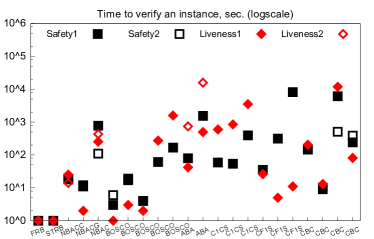
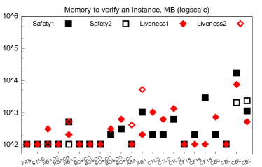
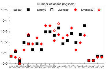
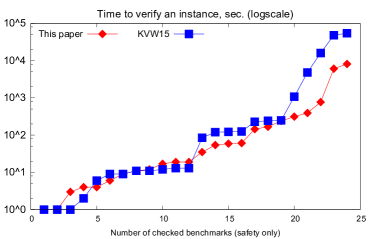
Figure 11: The plots summarize the following results of running our implementation on all benchmarks: used time in seconds (top left), used memory in megabytes (top right), the number of checked lassos (bottom left), time used both by our implementation and Konnov et al. [2015] to check safety only (bottom right). Several occurrences of the same benchmark correspond to different cases, such as $f>1$, $f=1$, and $f=0$. Symbols $\blacksquare$ and $\square$ correspond to the safety properties of each benchmark, while symbols $\blacklozenge$ and $\lozenge$ correspond to the liveness properties.

The procedure check_node is called with a node $v$ of the graph ${\cal G}\cup{\cal H}$ as a parameter. It adds assertions that encode a finite path and constraints on the configurations of this path. The finite path leads from the configuration that corresponds to the node $v$ to the configuration that corresponds to $v$’s successor in the order $\prec$. The constraints depend on $v$’s origin: (a) $v$ labels a formula $\textsf{{F}}\,\psi$ in the syntax tree of $\varphi$, (b) $v$ carries a threshold guard from the set $\Phi^{\mathrm{rise}}\cup\Phi^{\mathrm{fall}}$, (c) $v$ denotes the loop start, or (d) $v$ denotes the loop end. In case (a), we add an SMT assertion that the current configuration satisfies the propositional formula $\mathit{prop}(\psi)$ (line 21), and add a sequence of rules that leads to $v$’s successor while maintaining the invariants $\psi_{\mathit{inv}}$ of the preceding nodes and the $v$’s invariant $\psi_{k+1}$ (line 22). In case (b), in line 27, we add a sequence of rules, one of which should unlock (resp. lock) the threshold guard in $v\in\Phi^{\mathrm{rise}}$ (resp. $v\in\Phi^{\mathrm{fall}}$). Then, in line 29, we add a sequence of rules that leads to a configuration of $v$’s successor. All added configurations are required to satisfy the current invariant $\psi_{\mathit{inv}}$. As the threshold guard in $v$ is now unlocked (resp. locked), we include the guard (resp. its negation) in the current context $\Omega$. In case (c), we store the current configuration as the loop start in the variable $\mathrm{fs}$ and, as in (a) and (b), add a sequence of rules leading to $v$’s successor. Finally, in case (d), we should have reached the ending configuration that coincides with the loop start. To this end, in line 39, we add the constraint that forces the counters of both configurations to be equal. At this point, all the necessary SMT constraints have been added, and we call SMT_sat to check whether there is an assignment that satisfies the constraints. If there is one, we report it as a lasso witnessing the $\textsf{ELTL}_{\textsf{FT}}$-formula $\varphi$ that consists of: the concrete parameter values, the values of the counters and shared variables for each configuration, and the acceleration factors. Otherwise, we report that there is no witness lasso for the formula $\varphi$.

The procedure push_segment constructs a sequence of currently unlocked rules, as in the case of reachability Konnov et al. [2015]. However, this sequence should be repeated several times, as required by Theorems 6.3 and 6.4. Moreover, the freshly added configurations are required to satisfy the current invariant $\psi_{\mathit{inv}}$.

7.3 Experiments

We extended the tool ByMC Konnov et al. [2015] with our technique and conducted experiments with the freely available benchmarks from Konnov et al. [2015]: folklore reliable broadcast (FRB) Chandra and Toueg [1996], consistent broadcast (STRB) Srikanth and Toueg [1987], asynchronous Byzantine agreement (ABA) Bracha and Toueg [1985], condition-based consensus (CBC) Mostéfaoui et al. [2003], non-blocking atomic commitment (NBAC and NBACC Raynal [1997] and NBACG Guerraoui [2002]), one-step consensus with zero degradation (CF1S Dobre and Suri [2006]), consensus in one communication step (C1CS Brasileiro et al. [2001]), and one-step Byzantine asynchronous consensus (BOSCO Song and van Renesse [2008]). These threshold-guarded fault-tolerant distributed algorithms are encoded in a parametric extension of Promela.

Negations of the safety and liveness specifications of our benchmarks — written in $\textsf{ELTL}_{\textsf{FT}}$ — follow three patterns: unsafety $\,\textsf{{E}}\,(p\wedge\textsf{{F}}\,q)$, non-termination $\,\textsf{{E}}\,(p\wedge\textsf{{G}}\,\textsf{{F}}\,r\wedge\textsf{{G}}\,q)$, and non-response $\,\textsf{{E}}\,(\textsf{{G}}\,\textsf{{F}}\,r\wedge\textsf{{F}}\,(p\wedge\textsf{{G}}\,q))$. The propositions $p$, $q$, and $r$ follow the syntax of $\mathit{pform}$ (cf. Table 1), e.g., $p\equiv\bigwedge_{\ell\in\mathit{Locs}_{1}}\kappa[\ell]=0$ and $q\equiv\bigvee_{\ell\in\mathit{Locs}_{2}}\kappa[\ell]\neq 0$ for some sets of locations $\mathit{Locs}_{1}$ and $\mathit{Locs}_{2}$.

The results of our experiments are summarized in Figure 11. Given the properties of the distributed algorithms found in the literature, we checked for each benchmark one or two safety properties (depicted with $\blacksquare$ and $\square$) and one or two liveness properties (depicted with $\blacklozenge$ and $\lozenge$). For each benchmark, we display the running times and the memory used together by ByMC and the SMT solver Z3 De Moura and Bjørner [2008], as well as the number of exercised lasso shapes as discussed in Section 5.

For safety properties, we compared our implementation against the implementation of Konnov et al. [2015]. The results are summarized the bottom right plot in Figure 11, which shows that there is no clear winner. For instance, our implementation is 170 times faster on BOSCO for the case $n>5t$. However, for the benchmark ABA we experienced a tenfold slowdown. In our experiments, attempts to improve the SMT encoding for liveness usually impaired safety results.

Our implementation has verified safety and liveness of all ten parameterized algorithms in less than a day. Moreover, the tool reports counterexamples to liveness of CF1S and BOSCO exactly for the cases predicted by the distributed algorithms literature, i.e., when there are not enough correct processes to reach consensus in one communication step. Noteworthy, liveness of only the two simplest benchmarks (STRB and FRB) had been automatically verified before John et al. [2013].

8 Conclusions

Parameterized verification approaches the problem of verifying systems of thousands of processes by proving correctness for all system sizes. Although the literature predominantly deals with safety, parameterized verification for liveness is of growing interest, and has been addressed mostly in the context of programs that solve mutual exclusion or dining philosophers Atig et al. [2012]; Farzan et al. [2016]; Pnueli et al. [2002]; Fang et al. [2006]. These techniques do not apply to fault-tolerant distributed algorithms that have arithmetic conditions on the fraction of faults, threshold guards, and typical specifications that evaluate a global system state.

Parameterized verification is in general undecidable Apt and Kozen [1986]. As recently surveyed by Bloem et al. Bloem et al. [2015], one can escape undecidability by restricting, e.g., communication semantics, local state space, the local control flow, or the temporal logic used for specifications. Hence, we make explicit the required restrictions. On the one hand, these restrictions still allow us to model fault-tolerant distributed algorithms and their specifications, and on the other hand, they give rise to a practical verification method. The restrictions are on the local control flow (loops) of processes (Section 2.1), as well as on the temporal operators and propositional formulas (Section 3). We conjecture that lifting these restrictions quite quickly leads to undecidability again. In addition, we justify our restrictions with the considerable number of benchmarks Chandra and Toueg [1996]; Srikanth and Toueg [1987]; Bracha and Toueg [1985]; Mostéfaoui et al. [2003]; Raynal [1997]; Guerraoui [2002]; Dobre and Suri [2006]; Brasileiro et al. [2001]; Song and van Renesse [2008] that fit into our fragment, and with the convincing experimental results from Figure 11.

Our main technical contribution is to combine and extend several important techniques: First, we extend the ideas by Etessami et al. Etessami et al. [2002] to reason about shapes of infinite executions of lasso shape. These executions are counterexample candidates. Then we extend reductions introduced by Lipton Lipton [1975] to deal with $\textsf{ELTL}_{\textsf{FT}}{}$ formulas. (Techniques that extend Lipton’s in other directions can be found in Cohen and Lamport [1998]; Doeppner [1977]; Lamport and Schneider [1989]; Elmas et al. [2009]; Flanagan et al. [2005]; Konnov et al. [2016b].) Our reduction is specific to threshold guards which are typical for fault-tolerant distributed algorithms and are found in domain-specific languages. Using on our reduction we apply acceleration Bardin et al. [2008]; Konnov et al. [2016b] in order to arrive at our short counterexample property.

Our short counterexample property implies a completeness threshold, that is, a bound $b$ that ensures that if no lasso of length up to $b$ is satisfying an $\textsf{ELTL}_{\textsf{FT}}$ formula, then there is no infinite path satisfying this formula. For linear temporal logic with the F  and G  operators, Kroening et al. Kroening et al. [2011] prove bounds on the completeness thresholds on the level of Büchi automata. Their bound involves the recurrence diameter of the transition systems, which is prohibitively large for counter systems. Similarly, the general method to transfer liveness with fairness to safety checking by Biere et al. Biere et al. [2002] leads to an exponential growth of the diameter, and thus to too large values of $b$. Hence, we decided to conduct an analysis on the level of threshold automata, accelerated counter systems, and a fragment of the temporal logic, which allows us to exploit specifics of the domain, and get bounds that can be used in practice.

Acceleration has been applied for parameterized verification by means of regular model checking Pnueli and Shahar [2000]; Bouajjani et al. [2004]; Abdulla et al. [1998]; Schuppan and Biere [2006]. As noted by Fisman et al. Fisman et al. [2008], to verify fault-tolerant distributed algorithms, one would have to intersect the regular languages that describe sets of states with context-free languages that enforce the resilience condition (e.g., $n>3t$). Our approach of reducing to SMT handles resilience conditions naturally in linear integer arithmetic.

There are two reasons for our restrictions in the temporal logic: On one hand, in our benchmarks, there is no need to find counterexamples that contain a configuration that satisfies ${\mathbf{\boldsymbol{\kappa}}}[\ell]=0\vee{\mathbf{\boldsymbol{\kappa}}}[\ell^{\prime}]=0$ for some $\ell,\ell^{\prime}\in{\mathcal{L}}$. One would only need such a formula to specify requirement that at least one process is at location $\ell$ and at least one process is at location $\ell^{\prime}$ (the disjunction would be negated in the specification), which is unnatural for fault-tolerant distributed algorithms. On the other hand, enriching our logic with $\bigvee_{i\in\mathit{Locs}}{\mathbf{\boldsymbol{\kappa}}}[i]=0$ allows one to express tests for zero in the counter system, which leads to undecidability Bloem et al. [2015]. For the same reason, we avoid disjunction, as it would allow one to indirectly express test for zero: ${\mathbf{\boldsymbol{\kappa}}}[\ell]=0\vee{\mathbf{\boldsymbol{\kappa}}}[\ell^{\prime}]=0$.

The restrictions we put on threshold automata are justified from a practical viewpoint of our application domain, namely, threshold-guarded fault-tolerant algorithms. We assumed that all the cycles in threshold automata are simple (while the benchmarks have only self-loops or cycles of length 2). As our analysis already is quite involved, these restrictions allow us to concentrate on our central results without obfuscating the notation and theoretical results. Still, from a theoretical viewpoint it might be interesting to relax the restrictions on cycles in the future.

More generally, these restrictions allowed us to develop a completely automated verification technique. In general, there is a trade-off between degree of automation and generality. Our method is completely automatic, but our input language cannot compete in generality with mechanized proof methods that rely heavily on human expertise, e.g., IVY Padon et al. [2016], Verdi Wilcox et al. [2015], IronFleet Hawblitzel et al. [2015], TLAPS Chaudhuri et al. [2010].

APPENDIX

Appendix A Specifications of fault-tolerant distributed algorithms

In this section, we summarize the specifications of fault-tolerant distributed algorithms, which we used to conduct the experiments. As our method receives a negation of the original specification, we give only the negated formulas in $\textsf{ELTL}_{\textsf{FT}}$.

Input	Case	Lasso length		Nr. of lassos				Time, seconds				Memory, GB
FTDA	(if more than one)	avg	max	S1	S2	L1	L2	S1	S2	L1	L2	S1	S2	L1	L2
FRB	—	17	29	5	–	5	5	1	–	1	1	0.1	–	0.1	0.1
STRB	—	72	128	14	–	4	18	1	–	1	1	0.1	–	0.1	0.1
NBACC	—	4608	4632	2	1	1	3	19	18	25	14	0.1	0.1	0.3	0.1
NBACG	—	148	221	90	90	19	–	12	11	2	–	0.1	0.1	0.1	–
NBAC	—	2489	7109	448	69	69	517	771	110	253	431	0.5	0.1	0.2	0.5
BOSCO	$\lfloor\frac{n+3t}{2}\rfloor+1=n-t$	423	506	20	20	69	–	3	6	1	–	0.1	0.1	0.1	–
BOSCO	$\lfloor\frac{n+3t}{2}\rfloor+1>n-t$	368	1112	70	70	251	–	19	17	3	–	0.1	0.1	0.1	–
BOSCO	$\lfloor\frac{n+3t}{2}\rfloor+1<n-t$	286	562	20	20	69	–	4	4	2	–	0.1	0.1	0.1	–
BOSCO	$n>5t\wedge f=0$	30	8982	924	–	3431	–	61	–	272	–	0.2	–	0.3	–
BOSCO	$n>7t$	180	11294	924	–	3431	–	167	–	1579	–	0.3	–	0.6	–
ABA	$\frac{n+t}{2}=2t+1$	850	1435	448	–	138	1172	79	–	42	738	0.1	–	0.1	0.4
ABA	$\frac{n+t}{2}>2t+1$	2112	3548	2100	–	502	5204	1536	–	496	15720	1.0	–	0.2	5.1
C1CS	$f=0$	463	4352	70	–	251	–	59	–	596	–	0.2	–	1.0	–
C1CS	$f=1$	1276	7143	140	–	448	–	54	–	846	–	0.2	–	0.6	–
C1CS	$f>1$	436	4492	630	–	2100	–	393	–	3507	–	0.6	–	1.3	–
CF1S	$f=0$	1191	2114	90	–	19	–	35	–	26	–	0.1	–	0.1	–
CF1S	$f=1$	787	1757	523	–	90	–	313	–	5	–	0.2	–	0.1	–
CF1S	$f>1$	2132	4993	3429	–	448	–	8125	–	11	–	2.8	–	0.1	–
CBC	$\lfloor\frac{n}{2}\rfloor<n-t\wedge f=0$	8168	8168	2	2	2	–	145	146	204	–	0.2	0.2	0.7	–
CBC	$\lfloor\frac{n}{2}\rfloor=n-t\wedge f=0$	1790	1790	2	2	2	–	9	10	13	–	0.1	0.1	0.1	–
CBC	$\lfloor\frac{n}{2}\rfloor<n-t\wedge f>0$	10213	12236	5	5	4	–	6072	508	11799	–	16.7	2.0	7.3	–
CBC	$\lfloor\frac{n}{2}\rfloor=n-t\wedge f>0$	2258	2708	5	5	4	–	240	387	81	–	1.1	2.3	0.5	–

Table 2: Summary of our experiments on Intel® Xeon® E5345, 4 cores, 48 GB. We apply the optimizations introduced in [Konnov et al., 2015, Sec. 4.4.]. A gray box highlights the benchmarks, for which the tool reports a counterexample.

Consistent broadcast (STRB).

The negated safety specification (S1) is as follows:

1. $\textsf{{E}}\,((\bigvee_{\ell:\ \ell.\textit{sv\/}\rule{0.0pt}{3.01389pt}=\mathrm{V1}}{\mathbf{\boldsymbol{\kappa}}}[\ell]\neq 0)\wedge\textsf{{F}}\,\bigvee_{\ell:\ \ell.\textit{sv\/}\rule{0.0pt}{3.01389pt}=\textrm{AC}}\kappa_{\ell}\neq 0)$.

All our benchmarks have similar fairness constraints, that is the property of reliable communication that requires the processes to eventually receive the messages from all other correct processes. The fairness constraint that encodes reliable communication for STRB is as follows: $\varphi_{rc}\equiv(\textit{nsnt\/}\rule{0.0pt}{4.30554pt}<t+1\vee\bigwedge_{\ell:\ \ell\in\alpha(\textit{rcvd\/}\rule{0.0pt}{3.01389pt}<t+1)}{\mathbf{\boldsymbol{\kappa}}}[\ell]=0)\wedge(\textit{nsnt\/}\rule{0.0pt}{4.30554pt}<n-t\vee\bigwedge_{\ell:\ \ell.\textit{rcvd\/}\rule{0.0pt}{3.01389pt}\in\alpha(x<n-t)}{\mathbf{\boldsymbol{\kappa}}}[\ell]=0)$, where $\alpha(x<n-t)$ is the set of abstract values produced by the parametric interval data abstraction John et al. [2013].

Using $\varphi_{rc}$, we write the liveness properties L1 and L2 as:

1. $\,\textsf{{E}}\,\big{(}\textsf{{G}}\,\textsf{{F}}\,\varphi_{rc}\wedge\bigwedge_{\ell:\ \ell.\textit{sv\/}\rule{0.0pt}{3.01389pt}=\mathrm{V0}}\kappa_{\ell}=0\wedge\textsf{{G}}\,\bigwedge_{\ell:\ \ell.\textit{sv\/}\rule{0.0pt}{3.01389pt}=\textrm{AC}}\kappa_{\ell}=0\big{)}$.

2. $\,\textsf{{E}}\,\big{(}\textsf{{G}}\,\textsf{{F}}\,\varphi_{rc}\wedge\textsf{{F}}\,\big{(}\bigvee_{\ell:\ \ell.\textit{sv\/}\rule{0.0pt}{3.01389pt}=\textrm{AC}}\kappa_{\ell}\neq 0\wedge\textsf{{G}}\,(\bigvee_{\ell:\ \ell.\textit{sv\/}\rule{0.0pt}{3.01389pt}\neq\textrm{AC}}\kappa_{\ell}\neq 0)\big{)}$.

Folklore Reliable Broadcast (FRB).

FRB has exactly the same specifications S1, L1, and L2 as STRB, but fewer local states.

Asynchronous Byzantine agreement (ABA).

ABA has exactly the same specifications S1, L1, and L2 as STRB, but more local states and guards. In addition to $\varphi_{\mathit{rc}}$, ABA has four fairness constraints that enforce local progress of enabled process transitions, e.g., $\textsf{{G}}\,\textsf{{F}}\,(\textit{nsnt\/}\rule{0.0pt}{4.30554pt}<2t+1\vee\bigwedge_{\ell:\ \ell.\textit{sv\/}\rule{0.0pt}{3.01389pt}=\textrm{RD}}{\mathbf{\boldsymbol{\kappa}}}[\ell]=0)$.

Condition-based consensus (CBC).

CBC has two unique initial local states, where the processes are initialized with values 0 and 1 respectively. In our encoding, the numbers of processes in these states are counted with $\kappa_{0}$ and $\kappa_{1}$. The negation of termination is defined as follows:

1. $\,\textsf{{E}}\,\big{(}\textsf{{G}}\,\textsf{{F}}\,\varphi_{rc}\wedge|\kappa_{0}-\kappa_{1}|>t\wedge\textsf{{G}}\,\bigvee_{\ell:\ \ell.\textit{sv\/}\rule{0.0pt}{3.01389pt}\not\in\{\textrm{AC},\textrm{CR}\}}\kappa_{\ell}\neq 0\big{)}$

The negations of validity and agreement are as follows:

1. $\textsf{{E}}\,((\bigvee_{\ell:\ \ell.\textit{sv\/}\rule{0.0pt}{3.01389pt}=\mathrm{V1}}{\mathbf{\boldsymbol{\kappa}}}[\ell]\neq 0)\wedge\textsf{{F}}\,\bigvee_{\ell:\ \ell.\textit{sv\/}\rule{0.0pt}{3.01389pt}=\textrm{AC0}}\kappa_{\ell}\neq 0)$

2. $\textsf{{E}}\,(|\kappa_{0}-\kappa_{1}|>t\wedge\textsf{{F}}\,(\bigvee_{\ell:\ \ell.\textit{sv\/}\rule{0.0pt}{3.01389pt}\in\{\textrm{AC0},\textrm{AC1}\}}\kappa_{\ell}\neq 0))$

Non-blocking atomic commit.

In addition to the fairness constraint $\varphi_{rc}$, NBAC, NBACC, NBACG use a fairness constraint $\varphi_{\mathit{fd}}$ on a failure detector defined as: $\bigwedge_{\ell:\ \ell.\mathit{some\_fail}=\mathit{true}}\kappa_{\ell}=0\wedge\textsf{{G}}\,(\bigwedge_{\ell:\ \ell.\textit{sv\/}\rule{0.0pt}{3.01389pt}=\textrm{CR}}\kappa_{\ell}=0)$.

The negation of termination is defined as follows:

1. $\,\textsf{{E}}\,(\textsf{{G}}\,\textsf{{F}}\,\varphi_{rc}\wedge\varphi_{fd}\wedge\textsf{{G}}\,\bigvee_{\ell:\ \ell.\textit{sv\/}\rule{0.0pt}{3.01389pt}\not\in\{\textrm{COMMIT},\textrm{ABORT},\textrm{CR}\}}\kappa_{\ell}\neq 0)$

The negations of abort-validity and agreement are as follows:

1. $\textsf{{E}}\,((\bigvee_{\ell:\ \ell.\textit{sv\/}\rule{0.0pt}{3.01389pt}=\textrm{NO}}{\mathbf{\boldsymbol{\kappa}}}[\ell]\neq 0)\wedge\textsf{{F}}\,\bigvee_{\ell:\ \ell.\textit{sv\/}\rule{0.0pt}{3.01389pt}=\textrm{COMMIT}}\kappa_{\ell}\neq 0)$.

2. $\textsf{{E}}\,(\textsf{{F}}\,(\bigvee_{\ell:\ \ell.\textit{sv\/}\rule{0.0pt}{3.01389pt}=\textrm{ABORT}}\kappa_{\ell}\neq 0\wedge\bigvee_{\ell:\ \ell.\textit{sv\/}\rule{0.0pt}{3.01389pt}=\textrm{COMMIT}}\kappa_{\ell}\neq 0))$.

CFCS and C1CS.

The negation of fast termination for value 0 is:

1. $\,\textsf{{E}}\,(\textsf{{G}}\,\textsf{{F}}\,\varphi_{rc}\wedge\bigwedge_{\ell:\ \ell.\textit{sv\/}\rule{0.0pt}{3.01389pt}\neq\textrm{V0}}\kappa_{\ell}=0\wedge\textsf{{G}}\,\bigvee_{\ell:\ \ell.\textit{sv\/}\rule{0.0pt}{3.01389pt}\not\in\{\textrm{D0},\textrm{CR}\}}\kappa_{\ell}\neq 0)$

The negation of one-step for value 0 is:

1. $\,\textsf{{E}}\,(\bigwedge_{\ell:\ \ell.\textit{sv\/}\rule{0.0pt}{3.01389pt}\neq\textrm{V0}}\kappa_{\ell}=0\wedge\textsf{{F}}\,\bigvee_{\ell:\ \ell.\textit{sv\/}\rule{0.0pt}{3.01389pt}\in\{\textrm{D1},\textrm{U0},\textrm{U1}\}}\kappa_{\ell}\neq 0)$

BOSCO Song and van Renesse [2008].

The negation of fast termination for value 0 is:

1. $\,\textsf{{E}}\,(\textsf{{G}}\,\textsf{{F}}\,\varphi_{rc}\wedge\bigwedge_{\ell:\ \ell.\textit{sv\/}\rule{0.0pt}{3.01389pt}\neq\textrm{V0}}\kappa_{\ell}=0\wedge\textsf{{G}}\,\bigvee_{\ell:\ \ell.\textit{sv\/}\rule{0.0pt}{3.01389pt}\not\in\{\textrm{D0},\textrm{CR}\}}\kappa_{\ell}\neq 0)$

The negations of Lemma 3 and Lemma 4 of Song and van Renesse [2008] are:

1. $\,\textsf{{E}}\,(\textsf{{F}}\,(\bigvee_{\ell:\ \ell.\textit{sv\/}\rule{0.0pt}{3.01389pt}=\textrm{D0}}\kappa_{\ell}\neq 0\wedge\bigvee_{\ell:\ \ell.\textit{sv\/}\rule{0.0pt}{3.01389pt}=\textrm{D1}}\kappa_{\ell}\neq 0))$

2. $\,\textsf{{E}}\,(\textsf{{F}}\,(\bigvee_{\ell:\ \ell.\textit{sv\/}\rule{0.0pt}{3.01389pt}=\textrm{D0}}\kappa_{\ell}\neq 0\wedge\bigvee_{\ell:\ \ell.\textit{sv\/}\rule{0.0pt}{3.01389pt}=\textrm{U1}}\kappa_{\ell}\neq 0))$

Appendix B Detailed Proofs for Section 4

Proposition 4.2. Given a threshold automaton TA and an $\textsf{ELTL}_{\textsf{FT}}{}$ formula $\varphi$, if $\textsf{Sys}(\textsf{TA})\models\,\textsf{{E}}\,\varphi$, then there are an initial configuration $\sigma_{1}\in I$ and a schedule $\tau\cdot\rho^{\omega}$ with the following properties:

1. the path satisfies the formula: $\textsf{path}(\sigma_{1},\tau\cdot\rho^{\omega})\models\varphi$,

2. application of $\rho$ forms a cycle: $\rho^{k}(\tau(\sigma_{1}))=\tau(\sigma_{1})$ for $k\geq 0$.

Proof.

We do not give details on Büchi automata and the construction by Vardi and Wolper, since this construction is well-known and can be found in the original paper Vardi and Wolper [1986] as well as in a number of textbooks, e.g., Clarke et al. [1999][Ch. 9] and Baier and Katoen [2008][Ch. 5].

Using the construction from Vardi and Wolper [1986], we translate the formula $\varphi$ into a Büchi automaton $B=(\emph{AP},Q,\Delta,Q^{0},F)$, which has a finite set $Q$ of states, a finite set $Q_{0}\subseteq Q$ of initial states, a finite set $F$ of accepting states, a finite alphabet AP of atomic propositions (which corresponds to the propositional formulas derived from $\mathit{pform}$), and the transition relation $\Delta\subseteq Q\times\emph{AP}\times Q$. The key property is that the automaton $B$ recognizes exactly those sequences of propositions that satisfy the formula $\varphi$.

Let $(\Sigma,I,R)$ be the counter system $\textsf{Sys}(\textsf{TA})$ as defined in Section 2.2. The system $\textsf{Sys}(\textsf{TA})$ is a transition system, so following Vardi and Wolper [1986] we can construct the product Büchi automaton $\textsf{Sys}(\textsf{TA})\otimes B$ that corresponds to the synchronous product of $\textsf{Sys}(\textsf{TA})$ and $B$. Formally, $\textsf{Sys}(\textsf{TA})\otimes B$ is the Büchi automaton $(\emph{AP},Q_{P},\Delta_{P},Q_{P}^{0},F_{P})$ defined as follows:

• The set of states $Q_{P}$ is the Cartesian product $(\Sigma\cup\{\iota\})\times Q$, where $\iota\not\in\Sigma$ is a dummy configuration, which is used to delay initialization of the counter system by one step.

• The set of initial states $Q^{0}_{P}$ is the Cartesian product $\{\iota\}\times Q^{0}$.

• The set of accepting states $F_{P}$ is the Cartesian product $\Sigma\times F$.

• The transition relation $\Delta_{P}$ includes the following triples:

  • an initial transition $((\iota,q_{0}),p,(\sigma,q))$ for $q_{0}\in Q_{0}$, $\sigma\in I$, and $q\in Q$ such that $(q_{0},p,q)\in\Delta$ and $\sigma\models p$.

  • a transition $((\sigma,q),p,(\sigma^{\prime},q^{\prime}))$ for $q,q^{\prime}\in Q$ and $\sigma,\sigma^{\prime}\in\Sigma$ such that $(q,p,q^{\prime})\in\Delta$ and $\sigma^{\prime}\models p$.

A run of the product automaton is an infinite sequence $(\iota,q_{0}),$ $(\sigma_{1},q_{1}),\dots,(\sigma_{i},q_{i}),\dots$ such that $((\iota,q_{0}),p_{0},(\sigma_{1},q_{1}))\in\Delta$ and $((\sigma_{i},q_{i}),p_{i},(\sigma_{i+1},q_{i+1}))\in\Delta$ for $i\geq 1$ and some propositions $p_{0},p_{1},\dots\in\mathit{AP}$. The run is accepting, if there is a state $(\sigma_{j},q_{j})\in F_{P}$ that appears infinitely often in the run.

In contrast to Vardi and Wolper [1986], the product automaton $\textsf{Sys}(\textsf{TA})\otimes B$ has infinitely many states. However, by Proposition 2.10, every path of $\textsf{Sys}(\textsf{TA})$ visits only finitely many states, and thus every run of the product automaton visits finitely many states too. Hence, in each run there are finitely many accepting states. Due to this, and since, by assumption, $\textsf{Sys}(\textsf{TA})\models\,\textsf{{E}}\,\varphi$, the product has an accepting run $(\iota,q_{0}),(\sigma_{1},q_{1}),\dots,(\sigma_{i},q_{i}),\dots$ with state $(\sigma_{j},q_{j})\in F_{P}$ appearing infinitely often for some $j\geq 1$. Hence, there is an index $k\geq 0$ such that $(\sigma_{j+k+1},q_{j+k+1})=(\sigma_{j},q_{j})$. Consequently, we construct a lasso run by taking the sequence of states $(\iota,q_{0}),(\sigma_{1},q_{1}),\dots,(\sigma_{j-1},q_{j-1})$ as a prefix and the sequence $(\sigma_{j},q_{j}),\dots,(\sigma_{j+k},q_{j+k})$ as a loop, which is repeated infinitely. This lasso run is also an accepting run of the product automaton.

It is immediate from the construction, that the infinite sequence $\sigma_{1},\dots,\sigma_{j-1},(\sigma_{j},\dots,\sigma_{j+k})^{\omega}$ corresponds to a path of $\textsf{Sys}(\textsf{TA})$ starting from an initial configuration $\sigma_{1}\in I$, and this path satisfies the formula $\varphi$. Thus, there are schedules $\tau=t_{1},\dots,t_{j-1}$ and $\rho=t_{j},\dots,t_{j+k}$ such that:

1. Schedule $\tau$ is applicable to $\sigma_{1}$ and the prefixes of $\tau$ visit the intermediate configurations:

   $$(t_{1},\dots,t_{i})(\sigma_{1})=\sigma_{i}\mbox{ for }1\leq i<j,$$

2. Schedule $\rho$ is applicable to $\sigma_{j}$, the prefixes of $\rho$ visit the intermediate configurations, and $\rho$ closes the loop:

   $$(t_{j},\dots,t_{m})(\sigma_{j})=\begin{cases}\sigma_{m},&\mbox{ when }j\leq m<j+k\\ \sigma_{j},&\mbox{ when }m=j+k.\end{cases}$$

The infinite schedule $\tau\cdot\rho^{\omega}$ is the required schedule. Indeed, $\textsf{path}(\sigma_{1},\tau\cdot\rho^{\omega})\models\varphi$ and $\rho^{i}(\tau(\sigma_{1}))=\tau(\sigma_{1})$ for $i\geq 0$. ∎

Proposition 4.10. Let $\varphi$ be an $\textsf{ELTL}_{\textsf{FT}}$ formula, $\sigma$ be a configuration and $\tau\cdot\rho^{\omega}$ be a lasso schedule applicable to $\sigma$ such that $\textsf{path}(\sigma,\tau\cdot\rho^{\omega})\models\varphi$ holds. There is a constant $K\geq 0$ and a cut function $\zeta$ such that for every $\left<\textsf{{F}}\,\psi,w\right>\in{\cal G}({\cal T}(\varphi))$ if $\zeta(w)$ cuts $(\tau\cdot\rho^{K})\cdot\rho$ into $\pi^{\prime}$ and $\pi^{\prime\prime}$, then $\psi$ is satisfied at the cut point, that is, $\textsf{path}(\pi^{\prime}(\sigma),\pi^{\prime\prime}\cdot\rho^{\omega})\models\psi$.

Proof.

For each node $\left<\textsf{{F}}\,\psi,w\right>\in{\cal T}(\varphi)$, we define an extreme appearance $\operatorname{\mathit{EA}}(w)$ as follows:

1. If there is an index $k\in\{|\tau|,\dots,|\tau|+|\rho|-1\}$ such that $k$ cuts $\tau\cdot\rho$ in $\tau\cdot\rho^{\prime}$ and $\rho^{\prime\prime}$, and it holds that $\textsf{path}((\tau\cdot\rho^{\prime})(\sigma),\rho^{\prime\prime}\cdot\rho^{\omega})\models\psi$, then we set $\operatorname{\mathit{EA}}(w)$ to the maximal such $k\geq|\tau|$.

2. Otherwise, we set $\operatorname{\mathit{EA}}(w)$ to the maximal $k<|\tau|$ such that $k$ cuts $\tau$ in $\tau^{\prime},\tau^{\prime\prime}$ and $\textsf{path}(\tau^{\prime}(\sigma),\tau^{\prime\prime}\cdot\rho^{\omega})\models\psi$. (Such $k$ exists, as the case 1 does not apply, it holds $\textsf{path}(\sigma,\tau\cdot\rho^{\omega})\models\textsf{{F}}\,\psi$, and since temporal formulas are connected only with the conjunction $\wedge$.)

Consider a topologically ordered sequence $v_{1},v_{2},\dots,v_{|{\cal V}_{{\cal G}}|}$ of the vertices of the cut graph ${\cal G}({\cal T}(\varphi))=({\cal V}_{{\cal G}},{\cal E}_{{\cal G}})$, that is, the condition $(v_{i},v_{j})\in{\cal E}_{{\cal G}}$ implies $i<j$ for $1\leq i,j\leq|{\cal V}_{{\cal G}}|$. Such a sequence exists, since the graph ${\cal G}({\cal T}(\varphi))$ is a directed acyclic graph. Let $\ell\in\{1,\dots,|{\cal V}_{{\cal G}}|\}$ be the index of the node $\mathsf{loop}_{\mathsf{start}}$, i.e., $v_{\ell}=\mathsf{loop}_{\mathsf{start}}$.

We unroll the loop $K=\ell-1$ times. Formally, for $1\leq i\leq|{\cal V}_{{\cal G}}|$, we set the cut point $\zeta(v_{i})$ as follows:

$$\zeta(v_{i})=\begin{cases}|\tau|+|\rho|\cdot K,&\mbox{ if }v_{i}=\mathsf{loop}_{\mathsf{start}}\\ |\tau|+|\rho|\cdot(K+1)-1,&\mbox{ if }v_{i}=\mathsf{loop}_{\mathsf{end}}\\ \operatorname{\mathit{EA}}(v_{i}),&\mbox{ if }\operatorname{\mathit{EA}}(v_{i})<|\tau|\\ \operatorname{\mathit{EA}}(v_{i})+|\rho|\cdot(i-1),&\mbox{ if }i<\ell\mbox{ and }|\tau|\leq\operatorname{\mathit{EA}}(v_{i})\\ \operatorname{\mathit{EA}}(v_{i})+|\rho|\cdot K,&\mbox{ if }i\geq\ell\end{cases}$$

It is easy to see that $\zeta$ satisfies Definition 4.9. By the construction of extreme appearances, for a node $\left<\textsf{{F}}\,\psi,w\right>$, the formula $\psi$ is satisfied at the extreme appearance $\operatorname{\mathit{EA}}(w)$. Since $\zeta(w)-\operatorname{\mathit{EA}}(w)=|\rho|\cdot i$ for some $i\geq 0$, it follows that if $\zeta(w)$ cuts $(\tau\cdot\rho^{K})\cdot\rho^{\omega}$ into $\pi^{\prime}$ and $\pi^{\prime\prime}$, then $\textsf{path}(\pi^{\prime}(\sigma),\pi^{\prime\prime}\cdot\rho^{\omega})\models\psi$ holds. ∎

Lemma B.1.

Let $\sigma$ be a configuration, $\tau\cdot\rho^{\omega}$ be a lasso schedule applicable to $\sigma$, and $\varphi$ be an $\textsf{ELTL}_{\textsf{FT}}$ formula. If an index $k<|\tau|$ cuts $\tau$ into $\pi^{\prime}$ and $\pi^{\prime\prime}$ and $\textsf{Cfgs}(\pi^{\prime}(\sigma),\pi^{\prime\prime}\cdot\rho)\models\varphi$ holds, then $\textsf{path}(\pi^{\prime}(\sigma),\pi^{\prime\prime}\cdot\rho^{\omega})\models\textsf{{G}}\,\varphi$ holds.

Proof.

From $\textsf{Cfgs}(\pi^{\prime}(\sigma),\pi^{\prime\prime}\cdot\rho)\models\varphi$, we immediately conclude that two subsets of $\textsf{Cfgs}(\pi^{\prime}(\sigma),\pi^{\prime\prime}\cdot\rho)$ also satisfy $\varphi$:

$$\textsf{Cfgs}(\pi^{\prime}(\sigma),\pi^{\prime\prime}) \models\varphi$$ (6)

$$\textsf{Cfgs}(\tau(\sigma),\rho) \models\varphi$$ (7)

Since $\tau\cdot\rho^{\omega}$ is a lasso schedule, we have $\rho^{i}(\tau(\sigma))=\tau(\sigma)$ for $i\geq 0$. From this and Equation (7), we conclude that $\textsf{path}(\tau(\sigma),\rho^{\omega})\models\textsf{{G}}\,\varphi$ holds. By combining this with Equation (6), we arrive at the required property $\textsf{path}(\pi^{\prime}(\sigma),\pi^{\prime\prime}\cdot\rho^{\omega})\models\textsf{{G}}\,\varphi$. ∎

Lemma B.2.

Let $\sigma$ be a configuration, $\tau\cdot\rho^{\omega}$ be a lasso schedule applicable to $\sigma$, and $\varphi$ be an $\textsf{ELTL}_{\textsf{FT}}$ formula. If an index $k:|\tau|\leq k<|\tau|+|\rho|$ cuts $\tau\cdot\rho$ into $\pi^{\prime}$ and $\pi^{\prime\prime}$ and $\textsf{Cfgs}(\tau(\sigma),\rho)\models\varphi$ holds, then $\textsf{path}(\pi^{\prime}(\sigma),\pi^{\prime\prime}\cdot\rho^{\omega})\models\textsf{{G}}\,\varphi$ holds.

Proof.

Since $\tau\cdot\rho^{\omega}$ is a lasso schedule, we have $\rho^{i}(\tau(\sigma))=\tau(\sigma)$ for $i\geq 0$. Thus, $\textsf{Cfgs}(\tau(\sigma),\rho)\models\varphi$ implies $\textsf{path}(\tau(\sigma),\rho^{\omega})\models\textsf{{G}}\,\varphi$. As $\textsf{path}(\pi^{\prime}(\sigma),\pi^{\prime\prime}\cdot\rho^{\omega})$ is a subsequence of $\textsf{path}(\tau(\sigma),\rho^{\omega})$, we arrive at $\textsf{path}(\pi^{\prime}(\sigma),\pi^{\prime\prime}\cdot\rho^{\omega})\models\textsf{{G}}\,\varphi$. ∎

Theorem 4.12. Let $\sigma$ be a configuration, $\tau\cdot\rho^{\omega}$ be a lasso applicable to $\sigma$, and $\varphi$ be an $\textsf{ELTL}_{\textsf{FT}}$ formula. If there is a witness of $\textsf{path}(\sigma,\tau\cdot\rho^{\omega})\models\varphi$, then the lasso $\tau\cdot\rho^{\omega}$ satisfies $\varphi$, that is $\textsf{path}(\sigma,\tau\cdot\rho^{\omega})\models\varphi$.

Proof.

Let the cut graph ${\cal G}({\cal T}(\varphi))$ be $({\cal V}_{{\cal G}},{\cal E}_{{\cal G}})$. We start with defining the notion of the parent cutpoint for a formula that has the form $\textsf{{G}}\,\psi$. Given a tree node $\left<\textsf{{G}}\,\psi,u.j\right>\in{\cal T}(\varphi)$ with $\psi\neq\mathit{true}$, we denote with $\operatorname{\mathit{p-node}}(u.j)$ the parent node $\left<\psi^{\prime},u\right>\in{\cal T}(\varphi)$. (By the definition of a canonical syntax tree, the formula $\textsf{{G}}\,\psi$ alone cannot be the formula of the root node.) Note that the id $u$ always points to either the root node, or a node of the form $\left<\textsf{{F}}\,\psi^{\prime\prime},u\right>$ for some formula $\psi^{\prime\prime}\in\textsf{ELTL}_{\textsf{FT}}$. We define the parent cutpoint as follows:

$$\operatorname{\mathit{p-cutpoint}}(w)=\begin{cases}\zeta(u),\mbox{ when }u\in{\cal V}_{{\cal G}},w=u.j\mbox{ for some }j\in{\mathbb{N}}_{0},\\ 0,\mbox{ otherwise}.\end{cases}$$

We prove the following statements about the intermediate tree nodes using structural induction on the tree ${\cal T}(\varphi)$:

1. for a node $\left<\textsf{{G}}\,\psi,w\right>$ with $\psi\neq\mathit{true}$, if $\operatorname{\mathit{p-cutpoint}}(w)$ cuts $\tau\cdot\rho$ into $\pi^{\prime}$ and $\pi^{\prime\prime}$, then $\textsf{path}(\pi^{\prime}(\sigma),\pi^{\prime\prime}\cdot\rho^{\omega})\models\textsf{{G}}\,\psi$.

2. for a node $\left<\textsf{{F}}\,\psi,w\right>$, if $\zeta(w)$ cuts $\tau\cdot\rho$ into $\pi^{\prime}$ and $\pi^{\prime\prime}$, then $\textsf{path}(\pi^{\prime}(\sigma),\pi^{\prime\prime}\cdot\rho^{\omega})\models\psi$.

Based on this we finally prove

1. for the root node $\left<\mathit{can}(\varphi),0\right>\in{\cal T}(\varphi)$, it holds that $\textsf{path}(\sigma,\tau\cdot\rho^{\omega})\models\mathit{can}(\varphi)$.

which establishes the theorem.

Proving (i).

Fix a tree node $\left<\textsf{{G}}\,\psi,w\right>$ with $\psi\neq\mathit{true}$. Let $\operatorname{\mathit{p-cutpoint}}(w)$ cut $\tau\cdot\rho$ into $\pi^{\prime}$ and $\pi^{\prime\prime}$. We have to show that $\textsf{path}(\pi^{\prime}(\sigma),\pi^{\prime\prime}\cdot\rho^{\omega})\models\textsf{{G}}\,\psi$. Since $\psi\neq\mathit{true}$, by the definition of a canonical formula, $\psi$ has the form $\psi_{0}\wedge\textsf{{F}}\,\psi_{1}\dots\textsf{{F}}\,\psi_{k}\wedge\textsf{{G}}\,\mathit{true}$ for some $k\geq 0$, a propositional formula $\psi_{0}$ and canonical formulas $\psi_{1},\dots,\psi_{k}$. It is sufficient to show that: (a) $\pi^{\prime}(\sigma)\models\textsf{{G}}\,\psi_{0}$, and (b) $\textsf{path}(\pi^{\prime}(\sigma),\pi^{\prime\prime}\cdot\rho^{\omega})\models\textsf{{G}}\,\textsf{{F}}\,\psi_{i}$ for $1\leq i\leq k$.

To show (a), we consider three cases:

1. Case: $\operatorname{\mathit{p-node}}(w)$ is the root and $\varphi$ is not of the form $\textsf{{F}}\,(\dots)$. Then $\mathit{can}(\varphi)=\dots\wedge\textsf{{G}}\,\psi$, and by Condition (C1) of Definition 4.11, we have $\textsf{Cfgs}(\sigma,\tau\cdot\rho)\models\mathit{prop}(\psi)$. As $\tau\cdot\rho^{\omega}$ is a lasso, i.e., $(\tau\cdot\rho^{k}(\sigma))=\tau(\sigma)$ for $k\geq 0$, we have that $\sigma\models\textsf{{G}}\,\mathit{prop}(\psi)$. From this, and $\mathit{prop}(\psi)=\psi_{0}$, we conclude that $\pi^{\prime}(\sigma)\models\textsf{{G}}\,\psi_{0}$, as $\operatorname{\mathit{p-cutpoint}}(w)=0$ and thus $\pi^{\prime}$ is the empty schedule.

2. Case: $\operatorname{\mathit{p-node}}(w)=\left<\textsf{{F}}\,\psi^{\prime\prime},u\right>$ for some $\psi^{\prime\prime}\in\textsf{ELTL}_{\textsf{FT}}$ and $u\in{\mathbb{N}}_{0}^{\omega}$, and $\zeta(u)<|\tau|$. In this case, $\psi^{\prime\prime}=\dots\wedge\textsf{{G}}\,\psi$. By Condition (C2) of Definition 4.11, $\textsf{Cfgs}(\pi^{\prime}(\sigma),\pi^{\prime\prime})\models\mathit{prop}(\psi)$. By noticing $\mathit{prop}(\psi)=\psi_{0}$ and applying Lemma B.1, we have $\textsf{path}(\pi^{\prime}(\sigma),\pi^{\prime\prime}\cdot\rho^{\omega})\models\textsf{{G}}\,\psi_{0}$.

3. Case: $\operatorname{\mathit{p-node}}(w)=\left<\textsf{{F}}\,\psi^{\prime\prime},u\right>$ for some $\psi^{\prime\prime}\in\textsf{ELTL}_{\textsf{FT}}$ and $u\in{\mathbb{N}}_{0}^{\omega}$, and $|\tau|\leq\zeta(u)<|\tau|+|\rho|$. In this case, $\psi^{\prime\prime}=\dots\wedge\textsf{{G}}\,\psi$. By Condition (C3) of Definition 4.11, $\textsf{Cfgs}(\tau(\sigma),\rho)\models\mathit{prop}(\psi)$. By noticing $\mathit{prop}(\psi)=\psi_{0}$ and applying Lemma B.2, we arrive at $\textsf{path}(\pi^{\prime}(\sigma),\pi^{\prime\prime}\cdot\rho^{\omega})\models\textsf{{G}}\,\psi_{0}$.

To show (b), we fix an index $i:1\leq i\leq k$ and prove $\textsf{path}(\pi^{\prime}(\sigma),\pi^{\prime\prime}\cdot\rho^{\omega})\models\textsf{{G}}\,\textsf{{F}}\,\psi_{i}$. Let $w_{i}$ be the node id of the $\psi$’s subformula $\textsf{{F}}\,\psi_{i}$ in the syntax tree ${\cal T}(\varphi)$. Note that $\left<\textsf{{F}}\,\psi_{i},w_{i}\right>$ is covered by a G -node, since it is created from a subformula of $\textsf{{G}}\,\psi$. Thus, $(\mathsf{loop}_{\mathsf{start}},w_{i})\in{\cal E}_{{\cal G}}$, and by the definition of the cut function $\zeta$, we have $\zeta(w_{i})\geq\zeta(\mathsf{loop}_{\mathsf{start}})\geq|\tau|$. Let $\zeta(w_{i})$ cut $\tau\cdot\rho$ in $\tau\cdot\beta^{\prime}$ and $\beta^{\prime\prime}$. By the inductive hypothesis, Point (ii) holds for the tree node $w_{i}$, and thus $\textsf{path}((\tau\cdot\beta^{\prime})(\sigma),\beta^{\prime\prime}\cdot\rho^{\omega})\models\psi_{i}$ holds. Since $\tau\cdot\rho^{\omega}$ is a lasso-shaped schedule, we have $\tau(\sigma)=(\tau\cdot\rho^{j})(\sigma)$ for $j\geq 0$, that is, the state $\tau(\sigma)$ occurs infinitely often in the path $\textsf{path}((\tau\cdot\beta^{\prime})(\sigma),\beta^{\prime\prime}\cdot\rho^{\omega})$. Hence, we arrive at:

$$\textsf{path}((\tau\cdot\beta^{\prime})(\sigma),\beta^{\prime\prime}\cdot\rho^{\omega})\models\textsf{{G}}\,\textsf{{F}}\,\psi_{i},\mbox{ for }1\leq i\leq k.$$

From (a) and (b), and the standard LTL property $(\textsf{{G}}\,A)\wedge(\textsf{{G}}\,B)\Rightarrow\textsf{{G}}\,(A\wedge B)$, Point (i) follows for the tree node $\left<\textsf{{G}}\,\psi,w\right>$.

Proving (ii).

Fix a tree node $\left<\textsf{{F}}\,\psi,w\right>$, and let $\zeta(w)$ cut $\tau\cdot\rho$ into $\pi^{\prime}$ and $\pi^{\prime\prime}$. We have to show that $\textsf{path}(\pi^{\prime}(\sigma),\pi^{\prime\prime}\cdot\rho^{\omega})\models\psi$ holds.

By the definition of a canonical formula, $\psi$ has the form $\psi_{0}\wedge\textsf{{F}}\,\psi_{1}\wedge\dots\wedge\textsf{{F}}\,\psi_{k}\wedge\textsf{{G}}\,\psi_{k+1}$ for some $k\geq 0$, a propositional formula $\psi_{0}$, canonical formulas $\psi_{1},\dots,\psi_{k}$, and a formula $\psi_{k+1}$ that is either a canonical formula, or equals $\mathit{true}$. We will show that: (a) $\pi^{\prime}(\sigma)\models\psi_{0}$, and (b) $\textsf{path}(\pi^{\prime}(\sigma),\pi^{\prime\prime}\cdot\rho^{\omega})\models\textsf{{G}}\,\psi_{k+1}$, and (c) $\textsf{path}(\pi^{\prime}(\sigma),\pi^{\prime\prime}\cdot\rho^{\omega})\models\textsf{{F}}\,\psi_{i}$ for $1\leq i\leq k$. From (a)–(c), the required statement immediately follows.

To show (a), we notice that there are two cases: $\zeta(w)<|\tau|$, or $\zeta(w)\geq|\tau|$. In these cases, either Assumption ((C2)) or Assumption ((C3)) implies that $\pi^{\prime}(\sigma)\models\psi_{0}$.

To show (b), we focus on the case $\psi_{k+1}\neq\mathit{true}$, as the case $\psi_{k+1}=\mathit{true}$ is trivial. Notice that by the definition of the syntax tree ${\cal T}(\varphi)$, the subformula $\textsf{{G}}\,\psi_{k+1}$ has the id $w.j$ for $j=k+1$, and thus $\operatorname{\mathit{p-cutpoint}}(w.j)=\zeta(w)$. Thus, $(b)$ follows directly from the inductive hypothesis (i), which has already been shown to hold for the tree node $\left<\textsf{{G}}\,\psi_{k+1},w.j\right>$.

To show (c), fix an index $i\in\{1,\dots,k\}$. Let $\zeta(w.i)$ cut $\tau\cdot\rho$ into $\beta^{\prime}$ and $\beta^{\prime\prime}$. The inductive hypothesis (ii) has been shown to hold for the tree node $\left<\textsf{{F}}\,\psi_{i},w.i\right>\in{\cal T}(\varphi)$, and thus we have:

$$\textsf{path}(\beta^{\prime}(\sigma),\beta^{\prime\prime}\cdot\rho^{\omega})\models\psi_{i}.$$ (8)

We consider three cases, based on whether $w$ and $w.i$ are covered by a G -node:

1. Case: neither $w$, nor $w.i$ is covered by a G -node. By the definition of the cut graph, $(w,w.i)\in{\cal E}_{{\cal G}}$, and thus by the definition of the cut function $\zeta$, it holds that $\zeta(w)\leq\zeta(w.i)$. From this and Equation (8), it follows that $\textsf{path}(\pi^{\prime}(\sigma),\pi^{\prime\prime}\cdot\rho^{\omega})\models\textsf{{F}}\,\psi_{i}$.

2. Case: $w.i$ is covered by a G -node. By the definition of the cut graph, the node $w.i$ has to be inside the loop: $(\mathsf{loop}_{\mathsf{start}},w.i)\in{\cal E}_{{\cal G}}$. Consequently, by the definition of the cut function $\zeta$, it holds that $\zeta(w.i)\geq|\tau|$. Let $\beta^{\prime}_{l}$ be the suffix of $\beta^{\prime}$ inside the loop, i.e., $\beta^{\prime}=\tau\cdot\beta^{\prime}_{l}$. As $\tau\cdot\rho^{\omega}$ is a lasso-shaped schedule, we have $(\tau\cdot\rho\cdot\beta^{\prime}_{l})(\sigma)=\beta^{\prime}(\sigma)$. Consequently, we can advance one iteration of the loop and derive the following from Equation (8):

   $$\textsf{path}((\tau\cdot\rho\cdot\beta^{\prime}_{l})(\sigma),\beta^{\prime\prime}\cdot\rho^{\omega})\models\psi_{i}$$ (9)

   Notice that in Equation (9) we use $\tau\cdot\rho\cdot\beta^{\prime\prime}_{l}$, not $\tau\cdot\rho$. The definition of $\zeta$ requires that $\zeta(w)<|\tau|+|\rho|$. Since $|\tau\cdot\rho|\leq|\tau\cdot\rho\cdot\beta^{\prime}_{l}|$, we have $\zeta(w)\leq|\tau\cdot\rho\cdot\beta^{\prime}_{l}|$, that is, the formula $\psi_{i}$ is satisfied at the state $(\tau\cdot\rho\cdot\beta^{\prime}_{l})(\sigma)$ that either coincides with the state $\pi^{\prime}(\sigma)$ or occurs after the state $\pi^{\prime}(\sigma)$ in the path $\textsf{path}(\pi^{\prime}(\sigma),\pi^{\prime\prime}\cdot\rho^{\omega})$. From this and Equation (9), we conclude that $\textsf{path}(\pi^{\prime}(\sigma),\pi^{\prime\prime}\cdot\rho^{\omega})\models\textsf{{F}}\,\psi_{i}$ holds.

3. Case: $w$ is covered by a G -node, while $w.i$ is not. This case is impossible, since the node with id $w.i$ is the child of the node with id $w$ in the syntax tree ${\cal T}(\varphi)$.

From (a)–(c), Point (ii) follows for the tree node $\left<\textsf{{F}}\,\psi,w\right>$.

Proving (iii).

Let $\mathit{can}(\varphi)\equiv\psi_{0}\wedge\textsf{{F}}\,\psi_{1}\wedge\dots\wedge\textsf{{F}}\,\psi_{k}\wedge\textsf{{G}}\,\psi_{k+1}$, for some $k\geq 0$, a propositional formula $\psi_{0}$, canonical formulas $\psi_{1},\dots,\psi_{k}$, and a formula $\psi_{k+1}$ that is either a canonical formula, or equals to $\mathit{true}$. We have to show $\textsf{path}(\sigma,\tau\cdot\rho^{\omega})\models\mathit{can}(\varphi)$. To this end, we will show that: (a) $\sigma\models\psi_{0}$, and (b) $\textsf{path}(\sigma,\tau\cdot\rho^{\omega})\models\textsf{{G}}\,\psi_{k+1}$, and (c) $\textsf{path}(\sigma,\tau\cdot\rho^{\omega})\models\textsf{{F}}\,\psi_{i}$ for $1\leq i\leq k$. From (a)–(c), the required statement immediately follows.

Point (a) follows directly from Condition (C1) of Definition 4.11.

To show (b), we focus on the case $\psi_{k+1}\neq\mathit{true}$, as the case $\psi_{k+1}=\mathit{true}$ is trivial. Notice that by the definition of the syntax tree ${\cal T}(\varphi)$, the subformula $\textsf{{G}}\,\psi_{k+1}$ has the id $0.j$ for $j=k+1$, and thus $\operatorname{\mathit{p-cutpoint}}(0.j)=0$, which cuts $\tau\cdot\rho$ into the empty schedule and $\tau\cdot\rho$ itself. Thus, $(b)$ follows directly from the inductive hypothesis (i), which has already been shown to hold for the tree node $\left<\textsf{{G}}\,\psi_{k+1},0.j\right>$.

To show (c), fix an index $i\in\{1,\dots,k\}$. Let $\zeta(0.i)$ cut $\tau\cdot\rho$ into $\beta^{\prime}$ and $\beta^{\prime\prime}$. The inductive hypothesis (ii) has been shown to hold for the tree node $\left<\textsf{{F}}\,\psi_{i},0.i\right>\in{\cal T}(\varphi)$, and thus we have:

$$\textsf{path}(\beta^{\prime}(\sigma),\beta^{\prime\prime}\cdot\rho^{\omega})\models\psi_{i}.$$ (10)

Since $\textsf{path}(\beta^{\prime}(\sigma),\beta^{\prime\prime}\cdot\rho^{\omega})$ is a suffix of $\textsf{path}(\sigma,\tau\cdot\rho^{\omega})$, from Equation 10, we immediately obtain the required statement: $\textsf{path}(\sigma,\tau\cdot\rho^{\omega})\models\textsf{{F}}\,\psi_{i}$.

By collecting Points (a)–(c), we immediately arrive at: $\textsf{path}(\sigma,\tau\cdot\rho^{\omega})\models\mathit{can}(\varphi)$. By Definition 4.5, the formula $\varphi$ is equivalent to $\mathit{can}(\varphi)$. This finishes the proof. ∎

Theorem 4.13. Let $\varphi$ be an $\textsf{ELTL}_{\textsf{FT}}$ formula, $\sigma$ be a configuration and $\tau\cdot\rho^{\omega}$ be a lasso applicable to $\sigma$ such that $\textsf{path}(\sigma,\tau\cdot\rho^{\omega})\models\varphi$ holds. There is a witness of $\textsf{path}(\sigma,(\tau\cdot\rho^{K})\cdot\rho^{\omega})\models\varphi$ for some $K\geq 0$.

Proof.

We apply Proposition 4.10 to find the required number $K\geq 0$ and the cut function $\zeta$. It remains to show that Conditions (C1)–(C3) of Definition 4.11 are satisfied for the configuration $\sigma$ and the lasso $(\tau\cdot\rho^{K})\cdot\rho^{\omega}$.

Showing Condition (C1).

This condition does not depend on the structure of $\zeta$. Let $\mathit{can}(\varphi)=\psi_{0}\wedge\textsf{{F}}\,\psi_{1}\wedge\dots\textsf{{F}}\,\psi_{k}\wedge\textsf{{G}}\,\psi_{k+1}$. Since $\textsf{path}(\sigma,(\tau\cdot\rho^{K})\cdot\rho^{\omega})\models\varphi$, we immediately have $\sigma\models\psi_{0}$ and $\textsf{path}(\sigma,(\tau\cdot\rho^{K})\cdot\rho^{\omega})\models\textsf{{G}}\,\psi_{k+1}$. By the semantics of LTL, the latter implies that for all configurations $\sigma^{\prime}$ visited by the path $\textsf{path}(\sigma,(\tau\cdot\rho^{K})\cdot\rho^{\omega})$, it holds that $\sigma^{\prime}\models\mathit{prop}(\psi_{k+1})$. Since $\textsf{path}(\sigma,(\tau\cdot\rho^{K})\cdot\rho)$ is a subsequence of $\textsf{path}(\sigma,(\tau\cdot\rho^{K})\cdot\rho^{\omega})$, we immediately arrive at $\textsf{Cfgs}(\sigma,(\tau\cdot\rho^{K})\cdot\rho)\models\mathit{prop}(\psi_{k+1})$.

Showing Conditions (C2) and (C3).

Let $\psi=\psi_{0}\wedge\textsf{{F}}\,\psi_{1}\wedge\dots\wedge\textsf{{F}}\,\psi_{k}\wedge\textsf{{G}}\,\psi_{k+1}$. Further, assume that $\zeta(v)$ cuts $(\tau\cdot\rho^{K})\cdot\rho$ into $\pi^{\prime}$ and $\pi^{\prime\prime}$. By Proposition 4.10, we have $\textsf{path}(\pi^{\prime}(\sigma),\pi^{\prime\prime}\cdot\rho^{\omega})\models\psi$. Thus, we have the following:

$$\textsf{path}(\pi^{\prime}(\sigma),\pi^{\prime\prime}\cdot\rho^{\omega}) \models\psi_{0}$$ (11)

$$\textsf{path}(\pi^{\prime}(\sigma),\pi^{\prime\prime}\cdot\rho^{\omega}) \models\textsf{{G}}\,\mathit{prop}(\psi_{k+1})$$ (12)

It remains to prove the specific statements about (C2) and (C3):

1. Case $\zeta(v)<|\tau\cdot\rho^{K}|$. We have to show Condition (C2).

   The path $\textsf{path}(\pi^{\prime}(\sigma),\pi^{\prime\prime})$ is a subsequence of $\textsf{path}(\pi^{\prime}(\sigma),\pi^{\prime\prime}\cdot\rho^{\omega})$. Thus, from Equation (12), we obtain that for every configuration $\sigma^{\prime}$ visited by the finite path $\textsf{path}(\pi^{\prime}(\sigma),\pi^{\prime\prime})$, it holds that $\sigma^{\prime}\models\mathit{prop}(\psi_{k+1})$. In other words:

   $$\textsf{Cfgs}(\pi^{\prime}(\sigma),\pi^{\prime\prime})\models\mathit{prop}(\psi_{k+1})$$ (13)

   Equations (11) and (13) give us Condition (C2).

2. Case $\zeta(v)\geq|\tau\cdot\rho^{K}|$. We have to show Condition (C3). In this case, $\pi^{\prime}=(\tau\cdot\rho^{K})\cdot\pi^{\prime}_{l}$ for some schedule $\pi^{\prime}_{l}$.

   Consider the configuration $\sigma^{\prime}=(\tau\cdot\rho^{K}\cdot\rho\cdot\pi^{\prime}_{l})(\sigma)$, that is, $\sigma^{\prime}$ is the result of applying to $\sigma$ the prefix $\tau\cdot\rho^{K}$, one iteration of the loop $\rho$, and then the first part of the loop $\pi^{\prime}_{l}$. The configuration $\sigma^{\prime}$ is located at the cut point $\zeta(v)$ in the loop, and the path $\textsf{path}(\sigma^{\prime},\pi^{\prime\prime}\cdot\pi^{\prime}_{l})$ reaches the same configuration again, i.e., $(\pi^{\prime\prime}\cdot\pi^{\prime}_{l})(\sigma^{\prime})=\sigma^{\prime}$. From Equation (12), we have that the propositional formula $\mathit{prop}(\psi_{k+1})$ holds on the path $\textsf{path}(\sigma^{\prime},\pi^{\prime\prime}\cdot\pi^{\prime}_{l})$. Since both paths $\textsf{path}(\sigma^{\prime},\pi^{\prime\prime}\cdot\pi^{\prime}_{l})$ and $\textsf{path}((\tau\cdot\rho^{K})(\sigma),\rho)$ visit all configurations of the loop, we have:

   $$\textsf{Cfgs}((\tau\cdot\rho^{K})(\sigma),\rho)\models\textsf{{G}}\,\mathit{prop}(\psi_{k+1})$$ (14)

   Equations (11) and (14) give us Condition (C3).

The theorem follows. ∎

Appendix C Detailed Proofs for Section 6

From now on we fix a threshold automaton $\textsf{TA}=({\mathcal{L}},{\mathcal{I}},\Gamma,$ $\Pi,$ ${\mathcal{R}},$ ${\textit{RC\/}\rule{0.0pt}{4.30554pt}})$ and conduct our analysis in Sections C.1 to C.4 for this TA.

C.1 Preliminaries

We start by formalizing the notion of a thread.

Definition C.1 (Thread).

For a configuration $\sigma$ and a schedule $\tau=\tau_{1}\cdot t_{1}\cdot\tau_{2}\cdot\ldots\cdot t_{k}\cdot\tau_{k+1}$ applicable to $\sigma$, we define the sequence of transitions $\vartheta=t_{1},\ldots,t_{k}$, $k>0$ to be a thread of $\sigma$ and $\tau$ if

1. $t_{i}.{\mathit{factor}}=1$, for every $1\leq i\leq k$,

2. $t_{i}.{\mathit{to}}=t_{i+1}.{\mathit{from}}$, for every $1\leq i<k$.

For thread $\vartheta$, by $\vartheta.{\mathit{from}}$ and $\vartheta.{\mathit{to}}$ we denote $t_{1}.{\mathit{from}}$ and $t_{k}.{\mathit{to}}$, respectively.

Definition C.2 (Naming, Projection, and Decomposition).

A naming is a function $\eta\colon{\mathbb{N}}\rightarrow{\mathbb{N}}$. For a schedule $\tau$, and a set $S\subseteq{\mathbb{N}}$, by ${\tau}|_{\eta,S}$ we denote the sequence of transitions $\tau[j]$ satisfying $\eta(j)\in S$ that preserves the order of transitions from $\tau$, i.e., for all $j_{1},j_{2},l_{1},l_{2}$, $j_{1}<j_{2}$, if ${\tau}|_{\eta,S}[l_{1}]=\tau[j_{1}]$ and ${\tau}|_{\eta,S}[l_{2}]=\tau[j_{2}]$, then $l_{1}<l_{2}$. If $S$ is a one-element set $\{i\}$, we write ${\tau}|_{\eta,i}$ instead of ${\tau}|_{\eta,\{i\}}$. We use the notation $\Theta(\sigma,\tau,\eta)$ for the set $\{i\colon{\tau}|_{\eta,i}\text{ is a thread of }\sigma\text{ and }\tau\}$. For a configuration $\sigma$ and a schedule $\tau$, a naming is called a decomposition of $\sigma$ and $\tau$ if

1. for all $i\in{\mathbb{N}}$, ${\tau}|_{\eta,i}$ is a thread of $\sigma$ and $\tau$, or ${\tau}|_{\eta,i}$ is the empty sequence.

2. for all $\ell\in{\mathcal{L}}$, $\sigma.{\mathbf{\boldsymbol{\kappa}}}[\ell]\geq|\{i\colon i\in\Theta(\sigma,\tau,\eta)\wedge{\tau}|_{\eta,i}.{\mathit{from}}=\ell\}|$

Example C.3.

Let us reconsider Example 6.5 and Figure 9, with configuration $\sigma_{1}$ where $\sigma_{1}.{\mathbf{\boldsymbol{\kappa}}}[\ell_{0}]=\sigma_{1}.{\mathbf{\boldsymbol{\kappa}}}[\ell_{1}]=\sigma_{1}.{\mathbf{\boldsymbol{\kappa}}}[\ell_{2}]=1$ and $\sigma_{1}.{\mathbf{\boldsymbol{\kappa}}}[\ell_{3}]=0$, and the schedule $\tau=(r_{1},1),$ $(r_{6},1),$ $(r_{4},1),$ $(r_{2},1),$ $(r_{4},1)$. The function $\eta\colon{\mathbb{N}}\rightarrow{\mathbb{N}}$ with $\eta(1)=\eta(5)=1$, $\eta(2)=\eta(4)=2$, $\eta(3)=3$, and $\eta(k)=4$ for every $k\geq 6$, is a naming. We will now see that $\eta$ is a decomposition by checking the two points.

(1) Since $\eta(1)=\eta(5)=1$, the projection ${\tau}|_{\eta,1}$ consists of the first and the fifth transition, in that particular order, i.e., ${\tau}|_{\eta,1}=(r_{1},1),(r_{4},1)$. This is a thread, as the factor of both transitions is $1$, and $r_{1}.{\mathit{to}}=\ell_{2}=r_{4}.{\mathit{from}}$. Similarly, ${\tau}|_{\eta,2}=(r_{6},1),(r_{2},1)$, and ${\tau}|_{\eta,3}=(r_{4},1)$ are threads. Besides, ${\tau}|_{\eta,4}$ is the empty sequence, as numbers mapping to 4 are $n\geq 6$, and $\tau$ has length 5, i.e., there is no transition $\tau[n]$ for $n\geq 6$. Further, for every $i>4$, ${\tau}|_{\eta,i}$ is the empty sequence, as there is no $m\in{\mathbb{N}}$, with $\eta(m)=i$. Thus, $\Theta(\sigma,\tau,\eta)=\{1,2,3\}$. Note that ${\tau}|_{\eta,{\mathbb{N}}\setminus\{2\}}={\tau}|_{\eta,\{1,3\}}=(r_{1},1),(r_{4},1),(r_{4},1).$

(2) As ${\tau}|_{\eta,2}=r_{6}.{\mathit{from}}=\ell_{0}$, we obtain $\{i\colon i\in\Theta(\sigma,\tau,\eta)\wedge{\tau}|_{\eta,i}.{\mathit{from}}=\ell_{0}\}=\{2\}$, and $\sigma_{1}.{\mathbf{\boldsymbol{\kappa}}}[\ell_{0}]=1\geq|\{2\}|$. Similarly we check this inequality for other local states, and conclude that $\eta$ is a decomposition of $\sigma_{1}$ and $\tau$. $\triangleleft$

Proposition C.4.

If $\sigma$ is a configuration, $\tau$ is a steady schedule applicable to $\sigma$, and $\eta$ is a decomposition of $\sigma$ and $\tau$, then for each prefix $\tau^{\prime}$ of $\tau$, the naming $\eta$ is a decomposition of $\sigma$ and $\tau^{\prime}$. Further $\Theta(\sigma,\tau^{\prime},\eta)\subseteq\Theta(\sigma,\tau,\eta)$.

From [Konnov et al., 2016b, Prop. 12] we directly obtain:

Proposition C.5.

If $\sigma$ is a configuration, $\tau$ is a steady schedule applicable to $\sigma$, and $\eta$ is a decomposition of $\sigma$ and $\tau$, then for all $\ell$ in ${\mathcal{L}}$:

$$\tau(\sigma).{\mathbf{\boldsymbol{\kappa}}}[\ell]=\sigma.{\mathbf{\boldsymbol{\kappa}}}[\ell]+|\{i\colon i\in\Theta(\sigma,\tau,\eta)\wedge{\tau}|_{\eta,i}.{\mathit{to}}=\ell\}|\\ -|\{i\colon i\in\Theta(\sigma,\tau,\eta)\wedge{\tau}|_{\eta,i}.{\mathit{from}}=\ell\}|.$$

Proposition C.6.

If $\sigma$ is a configuration, $\tau$ is a steady conventional schedule applicable to $\sigma$, then there is a decomposition of $\sigma$ and $\tau$.

Proof.

We have to prove the two properties of Definition C.2. We do so by induction on the length of $\tau$.

• $|\tau|=1$. Let $\tau=t_{1}$ for a transition $t_{1}$, and let $\eta$ be the identity function. Then, ${\tau}|_{\eta,1}=t_{1}$ is a thread and for all $i>1$, the sequence ${\tau}|_{\eta,i}$ is empty. As $\tau$ is applicable to $\sigma$, $\sigma.{\mathbf{\boldsymbol{\kappa}}}[t_{1}.{\mathit{from}}]\geq 1$.

• $|\tau|>1$. Let $\tau=\tau^{\prime}\cdot t_{|\tau|}$, and let $\eta^{\prime}$ be a decomposition of $\sigma$ and $\tau^{\prime}$, which exists by the induction hypothesis. We distinguish two cases for $T=\{i\colon i\in\Theta(\sigma,\tau^{\prime},\eta^{\prime})\wedge{\tau^{\prime}}|_{\eta^{\prime},i}.{\mathit{to}}=t_{|\tau|}.{\mathit{from}}\}$:

  • If $T\neq\emptyset$, then for some $j\in T$ let

    $$\eta(k)=\begin{cases}j&\text{if }k=|\tau|\\ \eta^{\prime}(k)&\text{otherwise,}\end{cases}$$

    that is, we append transition $t_{|\tau|}$ to thread $j$. Therefore, $\Theta(\sigma,\tau,\eta)=\Theta(\sigma,\tau^{\prime},\eta^{\prime})$ and consequently for all $\ell\in{\mathcal{L}}$ we have $\{i\colon i\in\Theta(\sigma,\tau,\eta)\wedge{\tau}|_{\eta,i}.{\mathit{from}}=\ell\}=\{i\colon i\in\Theta(\sigma,\tau^{\prime},\eta^{\prime})\wedge{\tau^{\prime}}|_{\eta^{\prime},i}.{\mathit{from}}=\ell\}$. Hence, it follows from the induction hypothesis that for all $\ell\in{\mathcal{L}}$, $\sigma.{\mathbf{\boldsymbol{\kappa}}}[\ell]\geq|\{i\colon i\in\Theta(\sigma,\tau,\eta)\wedge{\tau}|_{\eta,i}.{\mathit{from}}=\ell\}|$.

  • If $T=\emptyset$, then for some $j\not\in\Theta(\sigma,\tau^{\prime},\eta^{\prime})$ let

    $$\eta(k)=\begin{cases}j&\text{if }k=|\tau|\\ \eta^{\prime}(k)&\text{otherwise,}\end{cases}$$

    that is, we add a new thread consisting of $t_{|\tau|}$ only. From applicability of $\tau$ to $\sigma$ follows that $\tau^{\prime}(\sigma).{\mathbf{\boldsymbol{\kappa}}}[t_{|\tau|}.{\mathit{from}}]\geq 1$. Now from Proposition C.5 follows that

    $$\sigma.{\mathbf{\boldsymbol{\kappa}}}[t_{|\tau|}.{\mathit{from}}]\geq 1-|T|+\\ +|\{i\colon i\in\Theta(\sigma,\tau^{\prime},\eta^{\prime})\wedge{\tau^{\prime}}|_{\eta^{\prime},i}.{\mathit{from}}=t_{|\tau|}.{\mathit{from}}\}|.$$

    As $|T|=0$ in this case and since by construction $|\{i\colon i\in\Theta(\sigma,\tau^{\prime},\eta^{\prime})\wedge{\tau^{\prime}}|_{\eta^{\prime},i}.{\mathit{from}}=t_{|\tau|}.{\mathit{from}}\}|=|\{i\colon i\in\Theta(\sigma,\tau,\eta)\wedge{\tau}|_{\eta,i}.{\mathit{from}}=t_{|\tau|}.{\mathit{from}}\}|-1$, we obtain that $\sigma.{\mathbf{\boldsymbol{\kappa}}}[t_{|\tau|}.{\mathit{from}}]\geq|\{i\colon i\in\Theta(\sigma,\tau,\eta)\wedge{\tau}|_{\eta,i}.{\mathit{from}}=t_{|\tau|}.{\mathit{from}}\}|$ as required. For the other components of $\sigma.{\mathbf{\boldsymbol{\kappa}}}$, the proposition follows from the induction hypothesis as $\Theta(\sigma,\tau,\eta)=\Theta(\sigma,\tau^{\prime},\eta^{\prime})\cup\{j\}$.

∎

Proposition C.7.

If $\sigma$ is a configuration, $\tau=\tau_{1}\cdot t_{i-1}\cdot t_{i}\cdot\tau_{2}$ is a steady schedule applicable to $\sigma$, $\eta$ is a decomposition of $\sigma$ and $\tau$, and $\eta(i-1)\neq\eta(i)$, then $\tau_{1}(\sigma).{\mathbf{\boldsymbol{\kappa}}}[t_{i}.{\mathit{from}}]\geq 1$.

Proof.

From Proposition C.5 follows that

$$\tau_{1}(\sigma).{\mathbf{\boldsymbol{\kappa}}}[t_{i}.{\mathit{from}}]=\sigma.{\mathbf{\boldsymbol{\kappa}}}[t_{i}.{\mathit{from}}]+|\{k\colon{\tau_{1}}|_{\eta,k}.{\mathit{to}}=t_{i}.{\mathit{from}}\}|\\ -|\{k\colon{\tau_{1}}|_{\eta,k}.{\mathit{from}}=t_{i}.{\mathit{from}}\}|.$$

We distinguish two cases:

• If $t_{i}={\tau}|_{\eta,\eta(i)}[1]$, that is, it is the first in the thread, then $|\{k\colon{\tau}|_{\eta,k}.{\mathit{from}}=t_{i}.{\mathit{from}}\}|>|\{k\colon{\tau_{1}}|_{\eta,k}.{\mathit{from}}=t_{i}.{\mathit{from}}\}|$. By assumption, $\sigma.{\mathbf{\boldsymbol{\kappa}}}[t_{i}.{\mathit{from}}]\geq|\{k\colon{\tau}|_{\eta,k}.{\mathit{from}}=t_{i}.{\mathit{from}}\}|$. Thus, $\tau_{1}(\sigma).{\mathbf{\boldsymbol{\kappa}}}[t_{i}.{\mathit{from}}]>|\{k\colon{\tau_{1}}|_{\eta,k}.{\mathit{to}}=t_{i}.{\mathit{from}}\}|\geq 0$, which proves the proposition in this case.

• Otherwise, by Definition C.2 (2), we have that $\sigma.{\mathbf{\boldsymbol{\kappa}}}[t_{i}.{\mathit{from}}]-|\{k\colon{\tau_{1}}|_{\eta,k}.{\mathit{from}}=t_{i}.{\mathit{from}}\}|\geq 0$. Therefore, it holds that $\tau_{1}(\sigma).{\mathbf{\boldsymbol{\kappa}}}[t_{i}.{\mathit{from}}]\geq|\{k\colon{\tau_{1}}|_{\eta,k}.{\mathit{to}}=t_{i}.{\mathit{from}}\}|$. As $\tau_{1}$ contains the prefix of ${\tau}|_{\eta,\eta(i)}$, we find that $|\{k\colon{\tau_{1}}|_{\eta,k}.{\mathit{to}}=t_{i}.{\mathit{from}}\}|\geq 1$ such that $\tau_{1}(\sigma).{\mathbf{\boldsymbol{\kappa}}}[t_{i}.{\mathit{from}}]\geq 1$ as required.

∎

Now we show that in a steady schedule, a transition of a thread commutes with transitions of other threads. This will allow us to move whole threads.

Definition C.8 (Move).

For a schedule $\tau$, and a natural number $i$, $1<i\leq|\tau|$, the schedule $\tau_{i{\scriptscriptstyle\leftarrow}}$ is obtained by moving the $i$th transition of $\tau$ to the left, and naming $\eta_{i{\scriptscriptstyle\leftarrow}}(k)$ is defined accordingly, for every $k\in{\mathbb{N}}$, i.e.,

$$\tau_{i{\scriptscriptstyle\leftarrow}}[k]=\begin{cases}\tau[i]&\text{if $k=i-1$}\\ \tau[i-1]&\text{if $k=i$}\\ \tau[k]&\text{otherwise,}\end{cases}$$

$$\eta_{i{\scriptscriptstyle\leftarrow}}(k)=\begin{cases}\eta(i)&\text{if $k=i-1$}\\ \eta(i-1)&\text{if $k=i$}\\ \eta(k)&\text{otherwise.}\end{cases}$$

For natural numbers $n$ and $m$, where $1\leq n\leq m\leq|\tau|$, we define $\tau_{n{\scriptscriptstyle\leftarrowtail}m}$ to be the schedule obtained from $\tau$ by moving the $m$th transition of $\tau$ to the $n$th position (that is $m-n$ times to the left), and naming $\eta_{n{\scriptscriptstyle\leftarrowtail}m}(k)$ accordingly, for every $k\in{\mathbb{N}}$, i.e.,

$$\tau_{n{\scriptscriptstyle\leftarrowtail}m}\,=\,(\ldots((\tau_{m{\scriptscriptstyle\leftarrow}})_{m-1{\scriptscriptstyle\leftarrow}})\ldots)_{n+1{\scriptscriptstyle\leftarrow}}\quad\mbox{ and}$$

$$\eta_{n{\scriptscriptstyle\leftarrowtail}m}(k)=(\ldots((\eta_{m{\scriptscriptstyle\leftarrow}})_{m-1{\scriptscriptstyle\leftarrow}})\ldots)_{n+1{\scriptscriptstyle\leftarrow}}(k).$$

Example C.9.

Note that if $m=n$, then $\tau_{n{\scriptscriptstyle\leftarrowtail}m}=\tau$ and $\eta_{n{\scriptscriptstyle\leftarrowtail}m}=\eta$. If $\tau=t_{1},t_{2},\ldots,t_{|\tau|}$, then for $i,n,m\in{\mathbb{N}}$ with $n<m\leq|\tau|$, and $i\leq|\tau|$, it is $\tau_{i{\scriptscriptstyle\leftarrow}}=t_{1},\ldots,t_{i-2},t_{i},t_{i-1},t_{i+1},\ldots,t_{|\tau|}$ and $\tau_{n{\scriptscriptstyle\leftarrowtail}m}=t_{1},\ldots,t_{n-1},t_{m},t_{n},t_{n+1},\ldots,t_{m-1},t_{m+1},\ldots,t_{|\tau|}$. $\triangleleft$

Proposition C.10.

If $\sigma$ is a configuration, $\tau$ is a steady schedule applicable to $\sigma$, and $\eta$ is a decomposition of $\sigma$ and $\tau$, then for every $i\in{\mathbb{N}}$, if $1<i\leq|\tau|$ and $\eta(i-1)\neq\eta(i)$, then

1. $\tau_{i{\scriptscriptstyle\leftarrow}}$ is a steady schedule applicable to $\sigma$,

2. $\eta_{i{\scriptscriptstyle\leftarrow}}$ is a decomposition of $\sigma$ and $\tau_{i{\scriptscriptstyle\leftarrow}}$, and ${\tau_{i{\scriptscriptstyle\leftarrow}}}|_{\eta_{i{\scriptscriptstyle\leftarrow}},j}={\tau}|_{\eta,j}$, for every $j\in\Theta(\sigma,\tau,\eta)$,

3. $\tau_{i{\scriptscriptstyle\leftarrow}}(\sigma)=\tau(\sigma)$.

Proof.

(1) To prove this we have to show that (1a) $\tau[i]$ is applicable to $\tau^{i-2}(\sigma)$, and that (1b) $\tau[i-1]$ is applicable to $\tau^{i-2}\cdot\tau[i](\sigma)$. Point (1) then follows from commutativity of addition and subtraction on the counters.

1. Since $\tau$ is a steady schedule, then it suffices to show that $\tau^{i-2}(\sigma).{\mathbf{\boldsymbol{\kappa}}}[\tau[i].{\mathit{from}}]\geq 1$, which follows from Proposition C.7.

2. If $\tau[i].{\mathit{from}}\neq\tau[i-1].{\mathit{from}}$, then $\tau^{i-2}\cdot\tau[i](\sigma).{\mathbf{\boldsymbol{\kappa}}}[\tau[i-1].{\mathit{from}}]\geq\tau^{i-2}(\sigma).{\mathbf{\boldsymbol{\kappa}}}[\tau[i-1].{\mathit{from}}]$ and the statement follows from applicability of $\tau$ to $\sigma$. Otherwise, from applicability of $\tau$ to $\sigma$ for the case $\tau[i-1].{\mathit{from}}=\tau[i-1].{\mathit{to}}$ it follows that $\tau^{i-2}(\sigma).{\mathbf{\boldsymbol{\kappa}}}[\tau[i-1].{\mathit{from}}]\geq 1$, and for $\tau[i-1].{\mathit{from}}\neq\tau[i-1].{\mathit{to}}$ it follows that $\tau^{i-2}(\sigma).{\mathbf{\boldsymbol{\kappa}}}[\tau[i-1].{\mathit{from}}]\geq 2$. In both cases the statement follows.

(2) We firstly show that every transition from ${\tau_{i{\scriptscriptstyle\leftarrow}}}|_{\eta_{i{\scriptscriptstyle\leftarrow}},j}$ is also in ${\tau}|_{\eta,j}$. Let $\tau_{i{\scriptscriptstyle\leftarrow}}[k]$ be a transition from ${\tau_{i{\scriptscriptstyle\leftarrow}}}|_{\eta_{i{\scriptscriptstyle\leftarrow}},j}$. Thus, $\eta_{i{\scriptscriptstyle\leftarrow}}(k)=j$. We want to show that $\tau_{i{\scriptscriptstyle\leftarrow}}[k]$ is also in ${\tau}|_{\eta,j}$. We consider three cases:

• If $k=i-1$, then $\tau_{i{\scriptscriptstyle\leftarrow}}[k]=\tau_{i{\scriptscriptstyle\leftarrow}}[i-1]=\tau[i]$ and $\eta(i)=\eta_{i{\scriptscriptstyle\leftarrow}}(i-1)=\eta_{i{\scriptscriptstyle\leftarrow}}(k)=j$. As $\eta(i)=j$, then $\tau[i]$ belongs to ${\tau}|_{\eta,j}$. Now $\tau[i]=\tau_{i{\scriptscriptstyle\leftarrow}}[k]$ gives the required.

• If $k=i$, then $\tau_{i{\scriptscriptstyle\leftarrow}}[k]=\tau_{i{\scriptscriptstyle\leftarrow}}[i]=\tau[i-1]$ and $\eta(i-1)=\eta_{i{\scriptscriptstyle\leftarrow}}(i)=\eta_{i{\scriptscriptstyle\leftarrow}}(k)=j$. As $\eta(i-1)=j$, then $\tau[i-1]=\tau_{i{\scriptscriptstyle\leftarrow}}[k]$ belongs to ${\tau}|_{\eta,j}$.

• If $k\neq i-1$ and $k\neq i$, then by Definition C.8 we have $\tau_{i{\scriptscriptstyle\leftarrow}}[k]=\tau[k]$ and $\eta(k)=\eta_{i{\scriptscriptstyle\leftarrow}}(k)=j$. Since $\eta(k)=j$, then $\tau[k]$ is in ${\tau}|_{\eta,j}$. Now $\tau[k]=\tau_{i{\scriptscriptstyle\leftarrow}}[k]$ gives the required.

Proving that every transition from ${\tau}|_{\eta,j}$ is also in ${\tau_{i{\scriptscriptstyle\leftarrow}}}|_{\eta_{i{\scriptscriptstyle\leftarrow}},j}$, is analogous to the previous direction.

Now we know that for every $j\in\Theta(\sigma,\tau,\eta)$, schedules ${\tau_{i{\scriptscriptstyle\leftarrow}}}|_{\eta_{i{\scriptscriptstyle\leftarrow}},j}$ and ${\tau}|_{\eta,j}$ contain same transitions. The order of these transitions remains the same, since the only two transitions with different positions in $\tau$ and $\tau_{i{\scriptscriptstyle\leftarrow}}$ are adjacent transitions from two different threads.

Now, knowing that $\eta$ is a decomposition of $\sigma$ and $\tau$, and that all threads remain the same, we conclude that $\eta_{i{\scriptscriptstyle\leftarrow}}$ is a decomposition of $\sigma$ and $\tau_{i{\scriptscriptstyle\leftarrow}}$.

(3) Follows from the step (2) and Proposition C.5. ∎

Proposition C.11.

Let $\sigma$ be a configuration, let $\tau$ be a steady schedule applicable to $\sigma$, and let $\eta$ be a decomposition of $\sigma$ and $\tau$. If for $n,m\in{\mathbb{N}}$ holds that $1\leq n\leq m\leq|\tau|$ and $\eta(m)\neq\eta(i)$, for every $i$ with $n\leq i<m$, then

1. $\tau_{n{\scriptscriptstyle\leftarrowtail}m}$ is a steady schedule applicable to $\sigma$,

2. $\eta_{n{\scriptscriptstyle\leftarrowtail}m}$ is a decomposition of $\sigma$ and $\tau_{n{\scriptscriptstyle\leftarrowtail}m}$, and ${\tau_{n{\scriptscriptstyle\leftarrowtail}m}}|_{\eta_{n{\scriptscriptstyle\leftarrowtail}m},j}={\tau}|_{\eta,j}$, for every $j\in\Theta(\sigma,\tau,\eta)$,

3. $\tau_{n{\scriptscriptstyle\leftarrowtail}m}(\sigma)=\tau(\sigma)$.

Proof.

This statement is a consequence of Proposition C.10 applied inductively $m-n$ times, as Definition C.8 suggests. In the case when $m=n$, the statement is trivially satisfied. ∎

Proposition C.12.

Let $\sigma$ be a configuration, let $\tau$ be a steady schedule applicable to $\sigma$, and let $\eta$ be a decomposition of $\sigma$ and $\tau$. Fix an $i\in\Theta(\sigma,\tau,\eta)$. Let us denote $\tau^{*}=\tau^{\prime}\cdot{\tau}|_{\eta,i}\cdot\tau^{\prime\prime}$, such that $\tau^{\prime}$ is a possibly empty prefix of $\tau$ which contains no transitions from ${\tau}|_{\eta,i}$, and $\tau^{\prime}\cdot\tau^{\prime\prime}={\tau}|_{\eta,{\mathbb{N}}\setminus\{i\}}$. Then

1. $\tau^{*}$ is a steady schedule applicable to $\sigma$,

2. there exists a decomposition $\eta^{*}$ of $\sigma$ and $\tau^{*}$ such that ${\tau^{*}}|_{\eta^{*},l}={\tau}|_{\eta,l}$, for every $l\in\Theta(\sigma,\tau,\eta)$.

3. $\tau^{*}(\sigma)=\tau(\sigma)$.

Proof.

Let us firstly enumerate all transitions from ${\tau}|_{\eta,i}$, for example, let ${\tau}|_{\eta,i}=t_{n_{1}},t_{n_{2}},\ldots,t_{n_{k}}$, for $1\leq n_{1}<n_{2}<\cdots<n_{k}\leq|\tau|$. Thus, $\tau^{\prime}=t_{1},\ldots,t_{s}$, for $0\leq s<n_{1}$. The idea is that we move transitions from ${\tau}|_{\eta,i}$, one by one, to the left, namely $t_{n_{1}}$ to the place $(s+1)$ in $\tau$, then $t_{n_{2}}$ to the place $s+2$, and so on, by repeatedly applying Proposition C.10, that preserves the required properties. Formally, $\tau^{*}=(\ldots((\tau_{s+1{\scriptscriptstyle\leftarrowtail}n_{1}})_{s+2{\scriptscriptstyle\leftarrowtail}n_{2}})\ldots)_{s+k{\scriptscriptstyle\leftarrowtail}n_{k}}$.

For every $j$ with $1\leq j\leq k$, we denote

$$\tau_{j}=(\ldots((\tau_{1{\scriptscriptstyle\leftarrowtail}n_{1}})_{2{\scriptscriptstyle\leftarrowtail}n_{2}})\ldots)_{j{\scriptscriptstyle\leftarrowtail}n_{j}}\mbox{ and }$$

$$\eta_{j}=(\ldots((\eta_{1{\scriptscriptstyle\leftarrowtail}n_{1}})_{2{\scriptscriptstyle\leftarrowtail}n_{2}})\ldots)_{j{\scriptscriptstyle\leftarrowtail}n_{j}}.$$

We prove by induction that for every $j$, with $1\leq j\leq k$, it holds that:

1. $\tau_{j}$ is a steady schedule applicable to $\sigma$,

2. $\eta_{j}$ is a decomposition of $\sigma$ and $\tau_{j}$, and ${\tau_{j}}|_{\eta_{j},l}={\tau}|_{\eta,l}$, for every $l\in\Theta(\sigma,\tau,\eta)$,

3. $\tau_{j}(\sigma)=\tau(\sigma)$.

If $j=1$, then $\tau_{j}=\tau_{s+1{\scriptscriptstyle\leftarrowtail}n_{1}}$. Note that $\eta(n_{1})\neq\eta(m)$, for every $m$ with $s+1\leq m<n_{1}$, since $t_{n_{1}}$ is the first transition in ${\tau}|_{\eta,i}$, or in other words, the smallest number mapped to $i$ by $\eta$. Now, as $1\leq s+1\leq n_{1}\leq|\tau|$, the required holds by Proposition C.11.

Assume that the statement holds for $j$, and let us show that then it holds for $j+1$ as well. Note that $\tau_{j+1}=(\tau_{j})_{(j+1){\scriptscriptstyle\leftarrowtail}n_{(j+1)}}$. We show that we can apply Proposition C.11 to $\sigma$, $\tau_{j}$, $\eta_{j}$, $s+j+1$ and $n_{j+1}$. By induction hypothesis, $\tau_{j}$ is a steady schedule applicable to $\sigma$, and $\eta_{j}$ is a decomposition of $\sigma$ and $\tau_{j}$. From the assumption that $1\leq s+1\leq n_{1}<n_{2}<\cdots<n_{k}\leq|\tau|$, follows that $1\leq s+j+1\leq n_{j+1}\leq|\tau|$. By construction, $\tau_{j}$ has a form $\tau^{\prime}\cdot t_{n_{1}}\cdot t_{n_{2}}\cdot\ldots\cdot t_{n_{j}}\cdot\rho_{1}\cdot t_{n_{j+1}}\cdot\rho_{2}$, where $\rho_{1}\cdot\rho_{2}=\tau^{\prime\prime}$. Note that no transition from $\rho_{1}$ is in ${\tau}|_{\eta,i}$, which is, by induction hypothesis, same as ${\tau_{j}}|_{\eta_{j},i}$. Thus, $\eta_{j}(n_{j+1})\neq\eta_{j}(m)$, for every $m$ with $s+j+1<m\leq n_{j+1}$. Now we can apply Proposition C.11, and obtain the required. ∎

Proposition C.13.

Let $\sigma$ be a configuration, let $\tau$ be a steady schedule applicable to $\sigma$, and let $\eta$ be a decomposition of $\sigma$ and $\tau$. If $i\in\Theta(\sigma,\tau,\eta)$, and we denote $\tau^{*}={\tau}|_{\eta,i}\cdot{\tau}|_{\eta,{\mathbb{N}}\setminus\{i\}}$, then

1. $\tau^{*}$ is a steady schedule applicable to $\sigma$,

2. there exists a decomposition $\eta^{*}$ of $\sigma$ and $\tau^{*}$ such that ${\tau^{*}}|_{\eta^{*},l}={\tau}|_{\eta,l}$, for every $l\in\Theta(\sigma,\tau,\eta)$,

3. $\tau^{*}(\sigma)=\tau(\sigma)$.

Proof.

This Proposition is a special case of Proposition C.12, when $\tau^{\prime}$ is the empty schedule. ∎

Proposition C.14.

Let $\sigma$ be a configuration, let $\tau$ be a steady schedule applicable to $\sigma$, and let $\eta$ be a decomposition of $\sigma$ and $\tau$. Fix $i,j\in\Theta(\sigma,\tau,\eta)$. If ${\tau}|_{\eta,j}$ can be written as ${\tau}|_{\eta,j}^{1}\cdot{\tau}|_{\eta,j}^{2}$, for some schedules ${\tau}|_{\eta,j}^{1}$ and ${\tau}|_{\eta,j}^{2}$, and if we denote

$$\tau^{*}={\tau}|_{\eta,j}^{1}\cdot{\tau}|_{\eta,i}\cdot{\tau}|_{\eta,j}^{2}\cdot{\tau}|_{\eta,{\mathbb{N}}\setminus\{i,j\}},$$

then the following holds:

1. $\tau^{*}$ is a steady schedule applicable to $\sigma$,

2. there exists a decomposition $\eta^{*}$ of $\sigma$ and $\tau^{*}$ such that ${\tau^{*}}|_{\eta^{*},i}={\tau}|_{\eta,i}$ and ${\tau^{*}}|_{\eta^{*},j}={\tau}|_{\eta,j}$, and

3. $\tau^{*}(\sigma)=\tau(\sigma)$.

Proof.

Firstly, we apply Proposition C.13 for configuration $\sigma$, schedule $\tau$, decomposition $\eta$ and $j\in\Theta(\sigma,\tau,\eta)$. Then we obtain schedule $\rho={\tau}|_{\eta,j}\cdot{\tau}|_{\eta,{\mathbb{N}}\setminus\{j\}}$ and decomposition $\eta_{\rho}$ of $\sigma$ and $\rho$. Then we apply Proposition C.12 for configuration $\sigma$, schedule $\rho$, decomposition $\eta_{\rho}$, $i\in\Theta(\sigma,\tau,\eta)$, and a prefix ${\tau}|_{\eta,j}^{1}$ of $\rho$ (as $\tau^{\prime}$ from the proposition). ∎

Until now, we discussed when transitions can be moved. In Konnov et al. [2015], the goal of this movings is to transform a schedule into a so-called representative schedule that reaches the same final configuration (cf. Example 6.2). These representative schedules are highly accelerated, and their length can be bounded. After some preliminary definitions, we recall how these representative schedules are constructed, and then give Proposition C.17 that establishes that representatives maintain an important trace property.

Given a threshold automaton $({\mathcal{L}},{\mathcal{I}},\Gamma,\Pi,{\mathcal{R}},{\textit{RC\/}\rule{0.0pt}{4.30554pt}})$, we define the precedence relation $\prec_{\scriptscriptstyle{\mathit{P}}}$: for a pair of rules $r_{1},r_{2}\in{\mathcal{R}}$, it holds that $r_{1}\prec_{\scriptscriptstyle{\mathit{P}}}r_{2}$ if and only if $r_{1}.{\mathit{to}}=r_{2}.{\mathit{from}}$. We denote by $\prec^{+}_{\scriptscriptstyle{\mathit{P}}}$ the transitive closure of $\prec_{\scriptscriptstyle{\mathit{P}}}$. Further, we say that $r_{1}\sim_{\scriptscriptstyle{\mathit{P}}}r_{2}$, if $r_{1}\prec^{+}_{\scriptscriptstyle{\mathit{P}}}r_{2}\,\wedge\,r_{2}\prec^{+}_{\scriptscriptstyle{\mathit{P}}}r_{1}$, or $r_{1}=r_{2}$. The relation $\sim_{\scriptscriptstyle{\mathit{P}}}$ defines equivalence classes of rules. For a given set of rules ${\mathcal{R}}$ let ${\mathcal{R}}/{\sim}$ be the set of equivalence classes defined by $\sim_{\scriptscriptstyle{\mathit{P}}}$. We denote by $[{r}]$ the equivalence class of rule $r$. For two classes $c_{1}$ and $c_{2}$ from ${\mathcal{R}}/{\sim}$ we write $c_{1}\prec_{\scriptscriptstyle{\mathit{C}}}c_{2}$ iff there are two rules $r_{1}$ and $r_{2}$ in ${\mathcal{R}}$ satisfying $[{r_{1}}]=c_{1}$ and $[{r_{2}}]=c_{2}$ and $r_{1}\prec^{+}_{\scriptscriptstyle{\mathit{P}}}r_{2}$ and $r_{1}\not\sim_{\scriptscriptstyle{\mathit{P}}}r_{2}$. As the relation $\prec_{\scriptscriptstyle{\mathit{C}}}$ is a strict partial order, there are linear extensions of $\prec_{\scriptscriptstyle{\mathit{C}}}$. We denote by $\prec^{\mathit{lin}}_{\scriptscriptstyle{\mathit{C}}}$ a linear extension of $\prec_{\scriptscriptstyle{\mathit{C}}}$.

Construction of Representative Schedule.

Given a configuration $\sigma$, and a steady schedule $\tau$ applicable to $\sigma$, $\mathsf{srep}[\sigma,\tau]$ is generated from $\tau$ by repeatedly swapping two neighboring transitions $t_{1}$ and $t_{2}$ if $[t_{2}]\prec^{\mathit{lin}}_{\scriptscriptstyle{\mathit{C}}}[t_{1}]$ until no more such transitions exist. Then all neighboring transitions that belong to the same rule are merged into a single (possibly accelerated) transition.

Then the transitions belonging to loops are replaced by a quite involved construction in [Konnov et al., 2015, Prop. 5]. As discussed in Section 2.1, in this paper we consider the restriction that loops are simple (there may be self-loops). Hence, we can have a simplified construction: If for some $j$, the rules $r_{1},r_{2},\dots,r_{j}$ build a loop, then all the transitions in the subschedule $\tau_{\mathrm{loop}}$ that belong to the loop are replaced by the schedule that is constructed as follows:

1. let $\sigma_{\mathrm{end}}=\tau_{\mathrm{loop}}(\sigma_{0})$

2. let $\tau^{\prime}=$ $(r_{1},f_{1}),$ $(r_{2},f_{2}),\dots,$ $(r_{j},f_{j}),$ $(r_{1},f_{j+1}),$ $(r_{2},f_{j+2}),$ $\dots$, $(r_{j},f_{2j})$ be the schedule that is obtained by

   • If $r_{1},\dots,r_{j}$ appear in $\tau_{\mathrm{loop}}$: inductively assigning values to the acceleration factors $f_{i}$, for $1\leq i\leq 2j$ as follows:

     • for $1\leq i\leq j$:
       $f_{i}=\sigma_{i-1}.{\mathbf{\boldsymbol{\kappa}}}[r_{i}.{\mathit{from}}]-\min(\sigma_{0}.{\mathbf{\boldsymbol{\kappa}}}[r_{i}.{\mathit{from}}],\sigma_{\mathrm{end}}.{\mathbf{\boldsymbol{\kappa}}}[r_{i}.{\mathit{from}}])$ and for $t_{i}=(r_{i},f_{i})$, we get $\sigma_{i}=t_{i}(\sigma_{i-1})$

     • for $j+1\leq i\leq 2j$:
       $f_{i}=\sigma_{i-1}.{\mathbf{\boldsymbol{\kappa}}}[r_{i-j}.{\mathit{from}}]-\sigma_{\mathrm{end}}.{\mathbf{\boldsymbol{\kappa}}}[r_{i-j}.{\mathit{from}}]$ and
       for $t_{i}=(r_{i},f_{i})$, we obtain $\sigma_{i}=t_{i}(\sigma_{i-1})$

   • otherwise, that is, if some rules are missing in the schedule, then we set their acceleration factors to zero. Note that due to the missing rules, the loop falls apart into several independent chains. Each of this chains is a subschedule of $\tau^{\prime}$, we just have to sum up the acceleration factors for the present rules. Formally, we proceed in two steps: First, if $r_{i}$ is not present in $\tau_{\mathrm{loop}}$, and for all $k<i$, $r_{k}$ is present in $\tau_{\mathrm{loop}}$ then $f_{\ell}=0$, for all $\ell$ that satisfy $\ell\leq i$ or $\ell\geq j+i$. Second, for $\ell$ with $i<\ell\leq j$, the factor $f_{\ell}$ is the sum of the acceleration factors of transitions in $\tau_{\mathrm{loop}}$ with the rule $r_{\ell}$. For $\ell$ with $j<\ell<i+j$, $f_{\ell}$ is the sum of the acceleration factors of transitions in $\tau_{\mathrm{loop}}$ with the rule $r_{\ell-j}$.

3. $\tau^{\prime\prime}$ is obtained from $\tau^{\prime}$ by removing all transitions with zero acceleration factors

4. we replace $\tau_{\mathrm{loop}}$ with $\tau^{\prime\prime}$.

Proposition C.15.

Let $\tau_{\mathrm{loop}}$ be a schedule applicable to $\sigma_{0}$ that consists of transitions whose rules all belong to the same loop. For all $\ell\in{\mathcal{L}}$, if $\sigma_{0}.{\mathbf{\boldsymbol{\kappa}}}[\ell]>0$ and $\tau_{\mathrm{loop}}(\sigma_{0}).{\mathbf{\boldsymbol{\kappa}}}[\ell]>0$, then $\textsf{Cfgs}(\sigma_{0},{\mathsf{srep}[\sigma_{0},\tau_{\mathrm{loop}}]})\models{\mathbf{\boldsymbol{\kappa}}}[\ell]>0$.

In this way, $\mathsf{srep}[\sigma,\tau]$ contains a subset of the rules of $\tau$ but ordered according to the linear extension $\prec^{\mathit{lin}}_{\scriptscriptstyle{\mathit{C}}}$ of the control flow of the automaton. Thus, from the above construction we directly obtain:

Proposition C.16.

Let $\sigma$ be a configuration and let $\tau$ be a steady schedule applicable to $\sigma$. The rules contained in transitions of $\mathsf{srep}[\sigma,\tau]$ are a subset of the rules contained in transitions of $\tau$.

From Proposition 6.1, we know that we can replace a schedule by its representative, and maintain the same final state. In the following propositions, we show that the representative schedule also maintains non-zero counters.

Proposition C.17.

Let $\sigma$ be a configuration, and let $\tau$ be a steady schedule applicable to $\sigma$. For every $\ell\in{\mathcal{L}}$, it holds that $\textsf{Cfgs}(\sigma,\tau)\models{\mathbf{\boldsymbol{\kappa}}}[\ell]>0$ implies $\textsf{Cfgs}(\sigma,\mathsf{srep}[\sigma,\tau])\models{\mathbf{\boldsymbol{\kappa}}}[\ell]>0.$

Proof.

Schedule $\mathsf{srep}[\sigma,\tau]$ is constructed by first swapping transitions and then reducing loops. We first show that swapping maintains ${\mathbf{\boldsymbol{\kappa}}}[\ell]>0$, and then that reducing loops does so, too.

Consider the sub-path $\sigma_{i-1},t_{i},\sigma_{i},t_{i+1},\sigma_{i+1}$ of one schedule in the construction and $\sigma_{i-1},t_{i+1},\sigma^{\prime}_{i},t_{i},\sigma_{i+1}$ be the path obtained by swapping. Assume by ways of contradiction that $\sigma_{i-1}.{\mathbf{\boldsymbol{\kappa}}}[\ell]>0$, $\sigma_{i}.{\mathbf{\boldsymbol{\kappa}}}[\ell]>0$, and $\sigma_{i+1}.{\mathbf{\boldsymbol{\kappa}}}[\ell]>0$, but $\sigma^{\prime}_{i}.{\mathbf{\boldsymbol{\kappa}}}[\ell]=0$. As ${\mathbf{\boldsymbol{\kappa}}}[\ell]$ reduces from $\sigma_{i-1}$ to $\sigma^{\prime}_{i}$, we get $t_{i+1}.{\mathit{from}}=\ell$. By similar reasoning on $\sigma^{\prime}_{i}$ and $\sigma_{i+1}$ we obtain $t_{i}.{\mathit{to}}=\ell$. It thus holds that $t_{i}\prec_{\scriptscriptstyle{\mathit{P}}}t_{i+1}$, which contradicts that these transitions are swapped in the construction of $\mathsf{srep}[\sigma,\tau]$.

Let $\dots,\sigma,\tau,\sigma^{\prime},\dots$ be the path before the loops are replaced and $\tau$ consist of all the transition belonging to one loop. From the above paragraph we know that $\sigma.{\mathbf{\boldsymbol{\kappa}}}[\ell]>0$ and $\sigma^{\prime}.{\mathbf{\boldsymbol{\kappa}}}[\ell]>0$. We may thus apply Proposition C.15 and the proposition follows. ∎

For threshold-guarded fault-tolerant algorithms, the restrictions we put on threshold automata are well justified. In this paper we used the assumption that all the cycles in threshold automata are simple. In fact this assumption is a generalization of the TAs we found in our benchmarks. The authors of Konnov et al. [2015] did not make this assumption. As a consequence, they have to explicitly treat contexts (the guards that currently evaluate to true), which lead to context-specific representative schedules. Our restriction allows us to use only one way to construct simple representative schedules (cf. Section C.1). In addition, with this restriction, we can easily proof Proposition C.16, while this proposition not true under the assumptions in Konnov et al. [2015]. We conjecture that even under their assumption a proposition similar to our Proposition C.17 can be proven, so that our results can be extended. As our analysis already is quite involved, these restrictions allow us to concentrate on our central results without obfuscating the notation and theoretical results. Still, from a theoretical viewpoint it might be interesting to lift the restrictions on loops.

We have now seen how to construct simple representative schedules. In the following Sections C.2 to C.4, we will see how we can construct representative schedules that maintain different forms of specifications.

C.2 Representative Schedules maintaining $\bigvee_{i\in\mathit{Locs}}{\mathbf{\boldsymbol{\kappa}}}[i]\neq 0$

Definition C.18 (Types).

Let $\sigma$ be a configuration, $\tau$ be a schedule applicable to $\sigma$, $\vartheta=t_{1},\ldots,t_{n}$ be a thread of $\sigma$ and $\tau$, $\mathrm{first}(\vartheta)=t_{1}.{\mathit{from}}$, $\mathrm{last}(\vartheta)=t_{n}.{\mathit{to}}$, $\mathrm{middle}(\vartheta)=\{t_{i}.{\mathit{to}}\colon 1\leq i<n\}$, and $\mathit{Locs}\subseteq{\mathcal{L}}$. We say that $\vartheta$ is of $\mathit{Locs}$-type:

• $A$, if $\{\mathrm{first}(\vartheta),\mathrm{last}(\vartheta)\}\cup\mathrm{middle}(\vartheta)\subseteq\mathit{Locs}$;

• $B$, if $\mathrm{first}(\vartheta)\in\mathit{Locs}$, $\mathrm{last}(\vartheta)\not\in\mathit{Locs}$;

• $C$, if $\mathrm{first}(\vartheta)\not\in\mathit{Locs}$, $\mathrm{last}(\vartheta)\in\mathit{Locs}$;

• $D$, if $\mathrm{first}(\vartheta)\not\in\mathit{Locs}$, $\mathrm{last}(\vartheta)\not\in\mathit{Locs}$, $\mathrm{middle}(\vartheta)\cap\mathit{Locs}\neq\emptyset$;

• $E$, if $\mathrm{first}(\vartheta)\in\mathit{Locs}$, $\mathrm{last}(\vartheta)\in\mathit{Locs}$, $\mathrm{middle}(\vartheta)\nsubseteq\mathit{Locs}$

• $F$, if $(\{\mathrm{first}(\vartheta),\mathrm{last}(\vartheta)\}\cup\mathrm{middle}(\vartheta))\cap\mathit{Locs}=\emptyset$.

Example C.19.

Let us consider the threshold automaton from Figure 9, and the subset of local states $\mathit{Locs}=\{\ell_{2}\}$. Schedule $(r_{4},1)$ is of $\mathit{Locs}$-type $B$, schedule $(r_{6},1),(r_{2},1)$ is of $\mathit{Locs}$-type $C$, and $(r_{1},1),(r_{4},1)$ is of $\mathit{Locs}$-type $D$. $\triangleleft$

Proposition C.20.

Given a configuration $\sigma$, a schedule $\tau$ applicable to $\sigma$, and a subset of local states $\mathit{Locs}$, every thread $\vartheta$ of $\sigma$ and $\tau$ is of exactly one $\mathit{Locs}$-type.

Proof.

We consider an arbitrary thread $\vartheta$ of $\sigma$ and $\tau$. There are two possibilities for $\mathrm{first}(\vartheta)$, namely, $\mathrm{first}(\vartheta)\in\mathit{Locs}$ or $\mathrm{first}(\vartheta)\not\in\mathit{Locs}$, and similarly for $\mathrm{last}(\vartheta)$, $\mathrm{last}(\vartheta)\in\mathit{Locs}$ or $\mathrm{last}(\vartheta)\not\in\mathit{Locs}$. Combining these possibilities, we obtain four cases:

• Assume $\mathrm{first}(\vartheta)\in\mathit{Locs}$ and $\mathrm{last}(\vartheta)\in\mathit{Locs}$. If $\mathrm{middle}(\vartheta)\subseteq\mathit{Locs}$, then $\vartheta$ is of $\mathit{Locs}$-type $A$. Otherwise, if $\mathrm{middle}(\vartheta)\nsubseteq\mathit{Locs}$, then $\vartheta$ is of $\mathit{Locs}$-type $E$.

• If $\mathrm{first}(\vartheta)\in\mathit{Locs}$ and $\mathrm{last}(\vartheta)\not\in\mathit{Locs}$, then $\vartheta$ is of $\mathit{Locs}$-type $B$.

• If $\mathrm{first}(\vartheta)\not\in\mathit{Locs}$ and $\mathrm{last}(\vartheta)\in\mathit{Locs}$, then $\vartheta$ is of $\mathit{Locs}$-type $C$.

• Finally, assume $\mathrm{first}(\vartheta)\not\in\mathit{Locs}$ and $\mathrm{last}(\vartheta)\not\in\mathit{Locs}$. If $\mathrm{middle}(\vartheta)\cap\mathit{Locs}\neq\emptyset$, then $\vartheta$ is of $\mathit{Locs}$-type $D$. Otherwise, if $\mathrm{middle}(\vartheta)\cap\mathit{Locs}=\emptyset$, then $\vartheta$ is of $\mathit{Locs}$-type $F$.

∎

Proposition C.21.

Let $\sigma$ be a configuration, and let $\tau$ be a steady conventional schedule applicable to $\sigma$. If there exists a decomposition $\eta$ of $\sigma$ and $\tau$ that satisfies $|\Theta(\sigma,\tau,\eta)|=1$ and $\tau$ is of $\mathit{Locs}$-type $A$, then $\mathsf{srep}[\sigma,\tau]$ is a thread of $\mathit{Locs}$-type $A$.

Proof.

By definition of a thread, the transitions in $\tau$ are ordered by the flow relation $\prec_{\scriptscriptstyle{\mathit{P}}}$. Due to our restriction of loops and the construction of representative schedules, $\mathsf{srep}[\sigma,\tau]$ does not contain rules that are not contained in $\tau$. Hence, no new intermediate states are added in the construction of $\mathsf{srep}[\sigma,\tau]$ which proves the proposition. ∎

Proposition C.22.

Let $\sigma$ be a configuration, and let $\tau$ be a steady conventional schedule applicable to $\sigma$. Fix a set $\mathit{Locs}\subseteq{\mathcal{L}}$. If there exists a decomposition $\eta$ of $\sigma$ and $\tau$ that satisfies $|\Theta(\sigma,\tau,\eta)|=1$ and $\tau$ is of $\mathit{Locs}$-type $A$, then $\textsf{Cfgs}(\sigma,\mathsf{srep}[\sigma,\tau])\models\bigvee_{\ell\in\mathit{Locs}}{\mathbf{\boldsymbol{\kappa}}}[\ell]\neq 0$.

Proof.

Let $\mathsf{srep}[\sigma,\tau]=t_{1},\ldots,t_{n}$, for an $n\in{\mathbb{N}}$. Since $\tau$ is of $\mathit{Locs}$-type $A$, by Proposition C.21, $\mathsf{srep}[\sigma,\tau]$ is of $\mathit{Locs}$-type $A$, which yields that for all $1\leq i\leq n$ both $t_{i}.{\mathit{from}}$ and $t_{i}.{\mathit{to}}$ are in $\mathit{Locs}$.

• Since $\mathsf{srep}[\sigma,\tau]$ is applicable to $\sigma$, it must be the case that $\sigma\models{\mathbf{\boldsymbol{\kappa}}}[\ell^{*}]\neq 0$, where $\ell^{*}=t_{1}.{\mathit{from}}\in\mathit{Locs}$.

• If $\tau^{\prime}=t_{1},\ldots,t_{k}$, $1\leq k\leq n$, is a nonempty prefix of $\mathsf{srep}[\sigma,\tau]$, then, by definition of a counter system from Section 2.2, we have that $\tau^{\prime}(\sigma).{\mathbf{\boldsymbol{\kappa}}}[t_{k}.{\mathit{to}}]>0$, and also $t_{k}.{\mathit{to}}\in\mathit{Locs}$.

Therefore, $\textsf{Cfgs}(\sigma,\mathsf{srep}[\sigma,\tau])\models\bigvee_{\ell\in\mathit{Locs}}{\mathbf{\boldsymbol{\kappa}}}[\ell]\neq 0$. ∎

Lemma C.23.

Let $\sigma$ be a configuration, let $\tau$ be a steady conventional schedule applicable to $\sigma$, and let $\eta$ be a decomposition of $\sigma$ and $\tau$. If $k\in\Theta(\sigma,\tau,\eta)$ and $n\in{\mathbb{N}}$ are such that $t_{n}$ is the last transition from ${\tau}|_{\eta,k}$, i.e., $n$ is the maximal number with $\eta(n)=k$, then for every prefix $\tau^{\prime}$ of $\tau$, of length $|\tau^{\prime}|\geq n$, we have that $\tau^{\prime}(\sigma).{\mathbf{\boldsymbol{\kappa}}}[\ell]\neq 0$, for $\ell=\mathrm{last}({\tau}|_{\eta,k})$.

Proof.

Fix a prefix $\tau^{\prime}$ of $\tau$ of length at least $n$. Then, by Proposition C.4, $\eta$ is a decomposition of $\sigma$ and $\tau^{\prime}$. Note that $k\in\Theta(\sigma,\tau^{\prime},\eta)$, and ${\tau}|_{\eta,k}={\tau^{\prime}}|_{\eta,k}$. Therefore ${\tau^{\prime}}|_{\eta,k}.{\mathit{to}}={\tau}|_{\eta,k}.{\mathit{to}}=t_{n}.{\mathit{to}}.$ Proposition C.5, when applied to $\tau^{\prime}$, yields

$$\tau^{\prime}(\sigma).{\mathbf{\boldsymbol{\kappa}}}[t_{n}.{\mathit{to}}]=\sigma.{\mathbf{\boldsymbol{\kappa}}}[t_{n}.{\mathit{to}}]\\ +|\{i\colon i\in\Theta(\sigma,\tau^{\prime},\eta)\wedge{\tau^{\prime}}|_{\eta,i}.{\mathit{to}}=t_{n}.{\mathit{to}}\}|\\ -|\{i\colon i\in\Theta(\sigma,\tau^{\prime},\eta)\wedge{\tau^{\prime}}|_{\eta,i}.{\mathit{from}}=t_{n}.{\mathit{to}}\}|$$

By Definition C.2, we have that $\sigma.{\mathbf{\boldsymbol{\kappa}}}[t_{n}.{\mathit{to}}]-|\{i\colon i\in\Theta(\sigma,\tau^{\prime},\eta)\wedge{\tau^{\prime}}|_{\eta,i}.{\mathit{from}}=t_{n}.{\mathit{to}}\}|\geq 0$. Since $\eta(n)=k\in\{i\colon i\in\Theta(\sigma,\tau^{\prime},\eta)\wedge{\tau^{\prime}}|_{\eta,i}.{\mathit{to}}=t_{n}.{\mathit{to}}\}$, we conclude that $|\{i\colon i\in\Theta(\sigma,\tau^{\prime},\eta)\wedge{\tau^{\prime}}|_{\eta,i}.{\mathit{to}}=t_{n}.{\mathit{to}}\}|\geq 1$. Thus $\tau^{\prime}(\sigma).{\mathbf{\boldsymbol{\kappa}}}[t_{n}.{\mathit{to}}]\geq~{}1$. ∎

Lemma C.24.

Let $\sigma$ be a configuration, let $\tau$ be a steady conventional schedule applicable to $\sigma$, and let $\eta$ be a decomposition of $\sigma$ and $\tau$. If $k\in\Theta(\sigma,\tau,\eta)$ and $n\in{\mathbb{N}}$ are such that $t_{n}$ is the first transition from ${\tau}|_{\eta,k}$, i.e., $n$ is the minimal number with $\eta(n)=k$, then for every prefix $\tau^{\prime}$ of $\tau$, of length $|\tau^{\prime}|<n$, we have that $\tau^{\prime}(\sigma).{\mathbf{\boldsymbol{\kappa}}}[\ell]\neq 0$, for $\ell=\mathrm{first}({\tau}|_{\eta,k}).$

Proof.

By repeated application of Proposition C.10, the first transition of ${\tau}|_{\eta,k}$ can be moved to the beginning of the schedule. Applying Proposition C.7 to the resulting schedule proves this lemma. ∎

Proposition C.25.

Let $\sigma$ be a configuration, let $\tau=t_{1},\ldots,t_{|\tau|}$ be a nonempty steady conventional schedule applicable to $\sigma$, and let $\eta$ be a decomposition of $\sigma$ and $\tau$. Fix a set $\mathit{Locs}$ of local states. If there is no local state $\ell\in\mathit{Locs}$ such that $\textsf{Cfgs}(\sigma,\tau)\models{\mathbf{\boldsymbol{\kappa}}}[\ell]\neq 0$, but it holds that $\textsf{Cfgs}(\sigma,\tau)\models\bigvee_{\ell\in\mathit{Locs}}\boldsymbol{\kappa}[\ell]\neq 0,$ then at least one of the following cases is true:

1. There is at least one thread of $\sigma$ and $\tau$, which is of $\mathit{Locs}$-type $A$;

2. There is a thread of $\mathit{Locs}$-type $B$ or $E$, and an additional of $\mathit{Locs}$-type $C$ or $E$;

3. There is a thread of $\mathit{Locs}$-type $E$, and one of $\mathit{Locs}$-type $D$.

Proof.

Firstly, if $|\Theta(\sigma,\tau,\eta)|=1$, we prove by contradiction that $\tau$ is of $\mathit{Locs}$-type $A$. Namely, if we suppose the opposite, we distinguish three cases:

• If $\tau$ is of $\mathit{Locs}$-type $C$, $D$ or $F$, then $\sigma\not\models\bigvee_{\ell\in\mathit{Locs}}{\mathbf{\boldsymbol{\kappa}}}[\ell]\neq 0$, and therefore $\textsf{Cfgs}(\sigma,\tau)\not\models\bigvee_{\ell\in\mathit{Locs}}\boldsymbol{\kappa}[\ell]\neq 0$;

• If $\tau$ is of $\mathit{Locs}$-type $B$, then $\tau(\sigma)\not\models\bigvee_{\ell\in\mathit{Locs}}{\mathbf{\boldsymbol{\kappa}}}[\ell]\neq 0$, and therefore again $\textsf{Cfgs}(\sigma,\tau)\not\models\bigvee_{\ell\in\mathit{Locs}}\boldsymbol{\kappa}[\ell]\neq 0$;

• If $\tau$ is of $\mathit{Locs}$-type $E$, and a $k$, $1\leq k<|\tau|$, is such that $t_{k}.{\mathit{to}}\not\in\mathit{Locs}$, then for the prefix $\tau^{\prime}$ of $\tau$ of length $k$ holds that $\tau^{\prime}(\sigma)\not\models\bigvee_{\ell\in\mathit{Locs}}{\mathbf{\boldsymbol{\kappa}}}[\ell]\neq 0$.

Thus, for all three options we get a contradiction, which tells us that $\tau$ cannot be of any other type, and leaves the only remaining option: that $\tau$ is of $\mathit{Locs}$-type $A$. This gives us the case 1.

Otherwise, if $|\Theta(\sigma,\tau,\eta)|\geq 2$, we have two options:

• If one of the threads is of $\mathit{Locs}$-type $A$, then this is the case $1$.

• If there is no thread of $\mathit{Locs}$-type $A$, we consider two possibilities:

  • There is a thread ${\tau}|_{\eta,i}$ of $\mathit{Locs}$-type $E$, for some $i\in\Theta(\sigma,\tau,\eta)$. Then, by definition, there is a $k\in{\mathbb{N}}$ such that $\eta(k)=i$ and $t_{k}.{\mathit{to}}\not\in\mathit{Locs}$. Assume by contradiction that we are not is cases 2. nor 3. Then, among the other threads, there are no threads of $\mathit{Locs}$-type $A$, $B$, $C$, $D$, nor $E$. In other words, all the other threads are of $\mathit{Locs}$-type $F$. Then the prefix $\tau^{\prime}$ of $\tau$ of length $k$ has the property that $\tau^{\prime}(\sigma)\not\models\bigvee_{\ell\in\mathit{Locs}}{\mathbf{\boldsymbol{\kappa}}}[\ell]\neq 0$. This is a contradiction with the assumption that $\textsf{Cfgs}(\sigma,\tau)\models\bigvee_{\ell\in\mathit{Locs}}\boldsymbol{\kappa}[\ell]\neq 0$.

  • There is no thread of $\mathit{Locs}$-type $E$. Since $\sigma\models\bigvee_{\ell\in\mathit{Locs}}{\mathbf{\boldsymbol{\kappa}}}[\ell]\neq 0$, there exists an $\ell^{\prime}\in\mathit{Locs}$ such that $\sigma\models{\mathbf{\boldsymbol{\kappa}}}[\ell^{\prime}]\neq 0$. From the assumption that $\textsf{Cfgs}(\sigma,\tau)\not\models{\mathbf{\boldsymbol{\kappa}}}[\ell^{\prime}]\neq 0$, we obtain that there must exist a thread $\vartheta_{1}$ with $\mathrm{first}(\vartheta_{1})=\ell^{\prime}\in\mathit{Locs}$. Since in this case there are no threads of $\mathit{Locs}$-type $A$ nor $E$, this implies that $\vartheta_{1}$ is of $\mathit{Locs}$-type $B$.

    Similarly, since $\tau(\sigma)\models\bigvee_{\ell\in\mathit{Locs}}{\mathbf{\boldsymbol{\kappa}}}[\ell]\neq 0$, there exists an $\ell^{\prime\prime}\in\mathit{Locs}$ such that $\tau(\sigma)\models{\mathbf{\boldsymbol{\kappa}}}[\ell^{\prime\prime}]\neq 0$. Now, from the assumption that $\textsf{Cfgs}(\sigma,\tau)\not\models{\mathbf{\boldsymbol{\kappa}}}[\ell^{\prime\prime}]\neq 0$, we obtain that there exists a thread $\vartheta_{2}$ with $\mathrm{last}(\vartheta_{2})=\ell^{\prime\prime}\in\mathit{Locs}$. Thus, $\vartheta_{2}$ is of $\mathit{Locs}$-type $C$, and this case is the case $2$.

Therefore, at least one of the given cases is true. ∎

Proposition C.26.

Let $\sigma$ be a configuration, let $\tau$ be a steady conventional schedule applicable to $\sigma$, and let $\eta$ be a decomposition of $\sigma$ and $\tau$. Fix a set $\mathit{Locs}$ of local states, and an $i\in\Theta(\sigma,\tau,\eta)$. If ${\tau}|_{\eta,i}$ is a thread of $\mathit{Locs}$-type $A$, and if we denote $\ell^{*}=\mathrm{last}({\tau}|_{\eta,i})$, then $\ell^{*}\in\mathit{Locs}$, and

$$\textsf{Cfgs}({\tau}|_{\eta,i}(\sigma),{\tau}|_{\eta,{\mathbb{N}}\setminus\{i\}})\models{\mathbf{\boldsymbol{\kappa}}}[\ell^{*}]\neq 0.$$

Proof.

Firstly note that ${\tau}|_{\eta,i}\cdot{\tau}|_{\eta,{\mathbb{N}}\setminus\{i\}}$ is a steady schedule applicable to $\sigma$, and ${\tau}|_{\eta,i}\cdot{\tau}|_{\eta,{\mathbb{N}}\setminus\{i\}}(\sigma)=\tau(\sigma)$, by Proposition C.13. Let $\tau^{\prime}$ be a prefix of ${\tau}|_{\eta,{\mathbb{N}}\setminus\{i\}}$. Then ${\tau}|_{\eta,i}\cdot\tau^{\prime}$ is a prefix of ${\tau}|_{\eta,i}\cdot{\tau}|_{\eta,{\mathbb{N}}\setminus\{i\}}$ of length $l\geq|{\tau}|_{\eta,i}|$. By Lemma C.23, it is ${\tau}|_{\eta,i}\cdot\tau^{\prime}(\sigma).{\mathbf{\boldsymbol{\kappa}}}[\ell^{*}]\neq 0$, where $\ell^{*}=\mathrm{last}({\tau}|_{\eta,i})$. As ${\tau}|_{\eta,i}$ is of $\mathit{Locs}$-type $A$, then $\ell^{*}\in\mathit{Locs}$. ∎

Proposition C.27.

Let $\sigma$ be a configuration, let $\tau$ be a steady conventional schedule applicable to $\sigma$, let $\eta$ be a decomposition of $\sigma$ and $\tau$, and let $\mathit{Locs}$ be a subset of ${\mathcal{L}}$. If $i,j\in\Theta(\sigma,\tau,\eta)$ are such that $i\neq j$, ${\tau}|_{\eta,i}$ is a thread of $\mathit{Locs}$-type $B$ or $E$, and ${\tau}|_{\eta,j}$ is a thread of $\mathit{Locs}$-type $C$ or $E$, then it holds that

1. $\textsf{Cfgs}(\sigma,{\tau}|_{\eta,j})\models{\mathbf{\boldsymbol{\kappa}}}[\ell_{1}]\neq 0$, for $\ell_{1}=\mathrm{first}({\tau}|_{\eta,i})\in\mathit{Locs}$,

2. $\textsf{Cfgs}({\tau}|_{\eta,j}(\sigma),{\tau}|_{\eta,{\mathbb{N}}\setminus\{j\}})\models{\mathbf{\boldsymbol{\kappa}}}[\ell_{2}]\neq 0,$ for $\ell_{2}=\mathrm{last}({\tau}|_{\eta,j})\in\mathit{Locs}$.

Proof.

Firstly note that ${\tau}|_{\eta,j}\cdot{\tau}|_{\eta,{\mathbb{N}}\setminus\{j\}}$ is a steady schedule applicable to $\sigma$, and ${\tau}|_{\eta,j}\cdot{\tau}|_{\eta,{\mathbb{N}}\setminus\{j\}}(\sigma)=\tau(\sigma)$, by Proposition C.13.

1) Let $\tau^{\prime}$ be a prefix of ${\tau}|_{\eta,j}$. Note that in this case $\tau^{\prime}$ is a prefix of ${\tau}|_{\eta,j}\cdot{\tau}|_{\eta,{\mathbb{N}}\setminus\{j\}}$ of length $l\leq|{\tau}|_{\eta,j}|$. From Lemma C.24 we obtain $\tau^{\prime}(\sigma)\models{\mathbf{\boldsymbol{\kappa}}}[\ell_{1}]\neq 0$, where $\ell_{1}=\mathrm{first}({\tau}|_{\eta,i})$. Since ${\tau}|_{\eta,i}$ is of type $B$ or $E$, we have that $\ell_{1}\in\mathit{Locs}$.

2) Let $\tau^{\prime}$ be a prefix of ${\tau}|_{\eta,{\mathbb{N}}\setminus\{j\}}$. In this case, ${\tau}|_{\eta,j}\cdot\tau^{\prime}$ is a prefix of ${\tau}|_{\eta,j}\cdot{\tau}|_{\eta,{\mathbb{N}}\setminus\{j\}}$ of length $l\geq|{\tau}|_{\eta,j}|$. By Lemma C.23 we have that ${\tau}|_{\eta,j}\cdot\tau^{\prime}(\sigma)\models{\mathbf{\boldsymbol{\kappa}}}[\ell_{2}]\neq 0$, or, equivalently, $\tau^{\prime}({\tau}|_{\eta,j}(\sigma))\models{\mathbf{\boldsymbol{\kappa}}}[\ell_{2}]\neq 0$, where $\ell_{2}=\mathrm{last}({\tau}|_{\eta,j})$. Since ${\tau}|_{\eta,j}$ is of $\mathit{Locs}$-type $C$ or $E$, then $\ell_{2}\in\mathit{Locs}$. ∎

Proposition C.28.

Let $\sigma$ be a configuration, let $\tau$ be a steady conventional schedule applicable to $\sigma$, and let $\eta$ be a decomposition of $\sigma$ and $\tau$. Fix a subset $\mathit{Locs}$ of ${\mathcal{L}}$. For $i,j\in\Theta(\sigma,\tau,\eta)$, let ${\tau}|_{\eta,i}$ be a thread of $\mathit{Locs}$-type $E$, and let ${\tau}|_{\eta,j}$ be a thread of $\mathit{Locs}$-type $D$. Let us write ${\tau}|_{\eta,j}$ as ${\tau}|_{\eta,j}^{1}\cdot{\tau}|_{\eta,j}^{2}$, where $\mathrm{last}({\tau}|_{\eta,j}^{1})\in\mathit{Locs}$. If we denote

$$\tau^{*}={\tau}|_{\eta,j}^{1}\cdot{\tau}|_{\eta,i}\cdot{\tau}|_{\eta,j}^{2}\cdot{\tau}|_{\eta,{\mathbb{N}}\setminus\{i,j\}},$$

then we obtain that

1. $\textsf{Cfgs}(\sigma,{\tau}|_{\eta,j}^{1})\models{\mathbf{\boldsymbol{\kappa}}}[\ell_{1}]\neq 0$, for $\ell_{1}=\mathrm{first}({\tau}|_{\eta,i})\in\mathit{Locs}$,

2. $\textsf{Cfgs}({\tau}|_{\eta,j}^{1}(\sigma),{\tau}|_{\eta,i})\models{\mathbf{\boldsymbol{\kappa}}}[\ell_{2}]\neq 0$, for $\ell_{2}=\mathrm{last}({\tau}|_{\eta,j}^{1})\in\mathit{Locs}$,

3. $\textsf{Cfgs}({\tau}|_{\eta,j}^{1}\cdot{\tau}|_{\eta,i}(\sigma),{\tau}|_{\eta,j}^{2}\cdot{\tau}|_{\eta,{\mathbb{N}}\setminus\{i,j\}})\models{\mathbf{\boldsymbol{\kappa}}}[\ell_{3}]\neq 0$, for $\ell_{3}=\mathrm{last}({\tau}|_{\eta,i})\in\mathit{Locs}$.

Proof.

By Proposition C.14, $\tau^{*}$ is a steady schedule applicable to $\sigma$, $\tau^{*}(\sigma)=\tau(\sigma)$, and there exists a decomposition $\eta^{*}$ of $\sigma$ and $\tau^{*}$ such that ${\tau}|_{\eta,i}={\tau^{*}}|_{\eta^{*},i}$ and ${\tau}|_{\eta,j}={\tau^{*}}|_{\eta^{*},j}$. Let $l_{1}=|{\tau}|_{\eta,j}^{1}|$ and $l_{2}=|{\tau}|_{\eta,i}|$.

1) Let $\tau^{\prime}$ be a prefix of ${\tau}|_{\eta,j}^{1}$, and therefore a prefix of $\tau^{*}$ of length $l\leq l_{1}$. By Lemma C.24, we have that $\tau^{\prime}(\sigma)\models{\mathbf{\boldsymbol{\kappa}}}[\ell_{1}]\neq 0$, where $\ell_{1}=\mathrm{first}({\tau}|_{\eta,i})$. Since ${\tau}|_{\eta,i}$ is of $\mathit{Locs}$-type $E$, it is $\ell_{1}\in\mathit{Locs}$.

2) Let $\tau^{\prime}$ be a prefix of ${\tau}|_{\eta,i}$. Then ${\tau}|_{\eta,j}^{1}\cdot\tau^{\prime}$ is a prefix of ${\tau}|_{\eta,j}^{1}\cdot{\tau}|_{\eta,i}$ of length $l\geq l_{1}$. We apply Lemma C.23 for the configuration $\sigma$, the schedule ${\tau}|_{\eta,j}^{1}\cdot{\tau}|_{\eta,i}$, and the decomposition $\eta^{*}$. With the decomposition $\eta^{*}$, schedule ${\tau}|_{\eta,j}^{1}$ is a thread of $\sigma$ and ${\tau}|_{\eta,j}^{1}\cdot{\tau}|_{\eta,i}$, and therefore from Lemma C.23 we obtain that ${\tau}|_{\eta,j}^{1}\cdot\tau^{\prime}(\sigma)\models{\mathbf{\boldsymbol{\kappa}}}[\ell_{2}]\neq 0$, or, equivalently, $\tau^{\prime}({\tau}|_{\eta,j}^{1}(\sigma))\models{\mathbf{\boldsymbol{\kappa}}}[\ell_{2}]\neq 0$, where $\ell_{2}=\mathrm{last}({\tau}|_{\eta,j}^{1})$. From the construction of ${\tau}|_{\eta,j}^{1}$ follows that $\ell_{2}\in\mathit{Locs}$.

3) Let $\tau^{\prime}$ be a prefix of ${\tau}|_{\eta,j}^{2}\cdot{\tau}|_{\eta,{\mathbb{N}}\setminus\{i,j\}}$. Then $\tau^{\prime\prime}={\tau}|_{\eta,i}\cdot\tau^{\prime}$ is a prefix of $\tau^{*}_{1}={\tau}|_{\eta,i}\cdot{\tau}|_{\eta,j}^{2}\cdot{\tau}|_{\eta,{\mathbb{N}}\setminus\{i,j\}}$ of length $l\geq l_{2}$. We define a naming $\eta_{1}$ of ${\tau}|_{\eta,j}^{1}(\sigma)$ and $\tau^{*}_{1}$, for every $n\in{\mathbb{N}}$, as follows:

$$\eta_{1}(n)=\eta^{*}(n+l_{1}).$$

Note that $\eta_{1}$ is a decomposition of ${\tau}|_{\eta,j}^{1}(\sigma)$ and $\tau^{*}_{1}$, and ${\tau^{*}_{1}}|_{\eta_{1},i}={\tau^{*}}|_{\eta^{*},i}={\tau}|_{\eta,i}$. We apply Lemma C.23 for the configuration ${\tau}|_{\eta,j}^{1}(\sigma)$, the schedule $\tau^{*}_{1}$, and the decomposition $\eta_{1}$, and obtain that for the prefix $\tau^{\prime\prime}$ of $\tau^{*}_{1}$ holds $\tau^{\prime\prime}({\tau}|_{\eta,j}^{1}(\sigma)).{\mathbf{\boldsymbol{\kappa}}}[\ell_{3}]\geq~{}1$, or, equivalently,

$$\tau^{\prime}({\tau}|_{\eta,i}({\tau}|_{\eta,j}^{1}(\sigma))).{\mathbf{\boldsymbol{\kappa}}}[\ell_{3}]\geq~{}1,$$

where $\ell_{3}=\mathrm{last}({\tau^{*}_{1}}|_{\eta_{1},i})=\mathrm{last}({\tau}|_{\eta,i})$. Again, as ${\tau}|_{\eta,i}$ is of $\mathit{Locs}$-type $E$, then $\ell_{3}\in\mathit{Locs}$. ∎

Proposition C.29.

Let $\sigma$ be a configuration, and let $\tau$ be a steady conventional schedule applicable to $\sigma$. Fix a set $\mathit{Locs}\subseteq{\mathcal{L}}$. If there exist a local state $\ell^{*}\in\mathit{Locs}$ such that $\textsf{Cfgs}(\sigma,\tau)\models{\mathbf{\boldsymbol{\kappa}}}[\ell^{*}]\neq 0$, then

$$\textsf{Cfgs}(\sigma,\mathsf{srep}[\sigma,\tau])\models\bigvee_{\ell\in\mathit{Locs}}{\mathbf{\boldsymbol{\kappa}}}[\ell]\neq 0.$$

Proof.

If there is a local state $\ell^{*}\in\mathit{Locs}$ such that $\textsf{Cfgs}(\sigma,\tau)\models{\mathbf{\boldsymbol{\kappa}}}[\ell^{*}]\neq 0$, then we have $\textsf{Cfgs}(\sigma,\mathsf{srep}[\sigma,\tau])\models{\mathbf{\boldsymbol{\kappa}}}[\ell^{*}]\neq 0$, by Proposition C.17. Therefore, $\textsf{Cfgs}(\sigma,\mathsf{srep}[\sigma,\tau])\models\bigvee_{\ell\in\mathit{Locs}}{\mathbf{\boldsymbol{\kappa}}}[\ell]\neq 0$. ∎

Proposition C.30.

Let $\sigma$ be a configuration, let $\tau=\tau_{1}\cdot\ldots\cdot\tau_{n}$, for $n\geq 1$, be a steady conventional schedule applicable to $\sigma$. Fix a set $\mathit{Locs}\subseteq{\mathcal{L}}$. If we denote $\tau^{*}=\mathsf{srep}[\sigma,\tau_{1}]\cdot\mathsf{srep}[\tau_{1}(\sigma),\tau_{2}]\cdot\ldots\cdot\mathsf{srep}[\tau_{1}\cdot\ldots\cdot\tau_{n-1}(\sigma),\tau_{n}]$, then the following holds:

• $\tau^{*}$ is applicable to $\sigma$, and $\tau^{*}(\sigma)=\tau(\sigma)$,

• $|\tau^{*}|\leq 2\cdot n\cdot|{\mathcal{R}}|.$

Proof.

Firstly note that for every $k$ with $1\leq k\leq n$, $\tau_{k}$ is a steady conventional schedule applicable to $\tau_{1}\cdot\ldots\cdot\tau_{k-1}(\sigma)$. Therefore, by Proposition 6.1, for every $k$ with $1\leq k\leq n$ holds that

• $\mathsf{srep}[\tau_{1}\cdot\ldots\cdot\tau_{k-1}(\sigma),\tau_{k}]$ is applicable to $\tau_{1}\cdot\ldots\cdot\tau_{k-1}(\sigma)$,

• $\mathsf{srep}[\tau_{1}\cdot\ldots\cdot\tau_{k-1}(\sigma),\tau_{k}](\tau_{1}\cdot\ldots\cdot\tau_{k-1}(\sigma))=\tau_{k}(\tau_{1}\cdot\ldots\cdot\tau_{k-1}(\sigma))=\tau_{1}\cdot\ldots\cdot\tau_{k}(\sigma)$,

• $|\mathsf{srep}[\tau_{1}\cdot\ldots\cdot\tau_{k-1}(\sigma),\tau_{k}]|\leq 2\cdot|{\mathcal{R}}|$.

The first two observations imply the statement a), and the third one implies b). ∎

Proposition C.31.

Let $\sigma$ be a configuration, let $\tau_{1}\cdot\ldots\cdot\tau_{n}$, for $n\geq 1$, be a steady conventional schedule applicable to $\sigma$ and let $\psi\equiv\bigvee_{\ell\in\mathit{Locs}}{\mathbf{\boldsymbol{\kappa}}}[\ell]\neq 0$. Fix a set $\mathit{Locs}\subseteq{\mathcal{L}}$. If for every $k$ with $1\leq k\leq n$ holds at least one of the following:

1. $\tau_{k}$ is a thread of $\sigma$ and $\tau_{1}\cdot\ldots\cdot\tau_{n}$ of $\mathit{Locs}$-type $A$,

2. $\textsf{Cfgs}(\tau_{1}\cdot\ldots\cdot\tau_{k-1}(\sigma),\tau_{k})\models{\mathbf{\boldsymbol{\kappa}}}[\ell]\neq 0$, for some $\ell\in\mathit{Locs}$,

then $\textsf{Cfgs}(\sigma,\tau^{*})\models\psi,$ for $\tau^{*}=\mathsf{srep}[\sigma,\tau_{1}]\cdot\mathsf{srep}[\tau_{1}(\sigma),\tau_{2}]\cdot\ldots\cdot\mathsf{srep}[\tau_{1}\cdot\ldots\cdot\tau_{n-1}(\sigma),\tau_{n}]$.

Proof.

For every $k$, $1\leq k\leq n$, we know that $\tau_{k}$ is a steady conventional schedule applicable to $\tau_{1}\cdot\ldots\cdot\tau_{k-1}(\sigma)$. We prove the statement by showing that for every $k$ with $1\leq k\leq n$ holds that

$$\textsf{Cfgs}(\tau_{1}\cdot\ldots\cdot\tau_{k-1}(\sigma),\mathsf{srep}[\tau_{1}\cdot\ldots\cdot\tau_{k-1}(\sigma),\tau_{k}])\models\psi.$$

If we fix one such $k$, then there are two cases:

• If $\tau_{k}$ is a thread of $\sigma$ and $\tau_{1}\cdot\ldots\cdot\tau_{n}$ of $\mathit{Locs}$-type $A$, then Proposition C.22 yields the required.

• If there exists an $\ell\in\mathit{Locs}$ such that $\textsf{Cfgs}(\tau_{1}\cdot\ldots\cdot\tau_{k-1}(\sigma),\tau_{k})\models{\mathbf{\boldsymbol{\kappa}}}[\ell]\neq 0$, then by Proposition C.17 we know that $\textsf{Cfgs}(\tau_{1}\cdot\ldots\cdot\tau_{k-1}(\sigma),\mathsf{srep}[\tau_{1}\cdot\ldots\cdot\tau_{k-1}(\sigma),\tau_{k}])\models{\mathbf{\boldsymbol{\kappa}}}[\ell]\neq 0,$ which implies the required.

∎

Proposition C.25 provides us with a case distinction. To prove the following theorem, for each of the cases we construct a representative schedule. We do so by repeatedly using Proposition C.10, to reorder transitions in the following way: In Case 1 we move the thread of $\mathit{Locs}$-type $A$ to the beginning of the schedule. Then, the representative schedule is obtained by applying Proposition 6.1 to the thread of $\mathit{Locs}$-type $A$ and then to the rest. In Case 2 we move the thread of $\mathit{Locs}$-type $C$ or $E$ to the beginning, and again apply Proposition 6.1 to the thread and the rest. Case 3 is the most involved construction. A prefix of the $\mathit{Locs}$-type $D$ thread is moved to the beginning followed by the complete $\mathit{Locs}$-type $E$ thread. Proposition 6.1 is applied to the prefix, the thread and the rest. If the assumption of the proposition is not satisfied (i.e., there is a local state $\ell\in\mathit{Locs}$ such that $\textsf{Cfgs}(\sigma,\tau)\models{\mathbf{\boldsymbol{\kappa}}}[\ell]\neq 0$), then we just apply Proposition 6.1 to $\tau$.

Theorem C.32.

Fix a threshold automaton $\textsf{TA}=({\mathcal{L}},$ ${\mathcal{I}},$ $\Gamma,$ $\Pi,$ ${\mathcal{R}},$ ${\textit{RC\/}\rule{0.0pt}{4.30554pt}})$, and a set $\mathit{Locs}\subseteq{\mathcal{L}}$. Let $\sigma$ be a configuration such that $\omega(\sigma)=\Omega$, and let $\psi\equiv\bigvee_{\ell\in\mathit{Locs}}{\mathbf{\boldsymbol{\kappa}}}[\ell]\neq 0$. Then for every steady conventional schedule $\tau$, applicable to $\sigma$, with $\textsf{Cfgs}(\sigma,\tau)\models\psi$, there is a steady schedule $\mathsf{repr}_{\vee}[\psi,\sigma,\tau]$ with the properties:

1. $\mathsf{repr}_{\vee}[\psi,\sigma,\tau]$ is applicable to $\sigma$, and $\mathsf{repr}_{\vee}[\psi,\sigma,\tau](\sigma)=\tau(\sigma)$,

2. $|\mathsf{repr}_{\vee}[\psi,\sigma,\tau]|\leq 6\cdot|{\mathcal{R}}|$,

3. $\textsf{Cfgs}(\sigma,\mathsf{repr}_{\vee}[\psi,\sigma,\tau])\models\psi$,

4. there exist $\tau_{1}$, $\tau_{2}$ and $\tau_{3}$, (not necessarily nonempty) subschedules of $\tau$, such that $\tau_{1}\cdot\tau_{2}\cdot\tau_{3}$ is applicable to $\sigma$, it holds that $\tau_{1}\cdot\tau_{2}\cdot\tau_{3}(\sigma)=\tau(\sigma)$, and $\mathsf{repr}_{\vee}[\psi,\sigma,\tau]=\mathsf{srep}[\sigma,\tau_{1}]\cdot\mathsf{srep}[\tau_{1}(\sigma),\tau_{2}]\cdot\mathsf{srep}[\tau_{1}\cdot\tau_{2}(\sigma),\tau_{3}]$.

Proof.

We give a constructive proof, and therefore $\tau_{1}$, $\tau_{2}$, $\tau_{3}$ and its properties will be obvious from the construction.

If there is a local state $\ell^{*}\in\mathit{Locs}$ such that $\textsf{Cfgs}(\sigma,\tau)\models{\mathbf{\boldsymbol{\kappa}}}[\ell^{*}]\neq 0$, by Proposition C.29 we have $\textsf{Cfgs}(\sigma,\mathsf{srep}[\sigma,\tau])\models\psi$. Using properties of $\mathsf{srep}[\sigma,\tau]$ described in Proposition 6.1, we see that the required schedule is

$$\mathsf{repr}_{\vee}[\psi,\sigma,\tau]=\mathsf{srep}[\sigma,\tau].$$

If this is not the case, and $\eta$ is a decomposition of $\sigma$ and $\tau$, then, since $\textsf{Cfgs}(\sigma,\tau)\models\psi$, by Proposition C.25 at least one of the following cases is true:

• Assume there is an $i\in\Theta(\sigma,\tau,\eta)$ such that ${\tau}|_{\eta,i}$ is of $\mathit{Locs}$-type $A$. We claim that the required schedule is

  $$\mathsf{repr}_{\vee}[\psi,\sigma,\tau]=\mathsf{srep}[\sigma,{\tau}|_{\eta,i}]\cdot\mathsf{srep}[{\tau}|_{\eta,i}(\sigma),{\tau}|_{\eta,{\mathbb{N}}\setminus\{i\}}].$$

  By Proposition C.13, ${\tau}|_{\eta,i}\cdot{\tau}|_{\eta,{\mathbb{N}}\setminus\{i\}}$ is a steady schedule applicable to $\sigma$, and ${\tau}|_{\eta,i}\cdot{\tau}|_{\eta,{\mathbb{N}}\setminus\{i\}}(\sigma)=\tau(\sigma)$. Therefore, we can apply Proposition C.30 to obtain a) and b). Since ${\tau}|_{\eta,i}$ is a thread of $\sigma$ and $\tau$, of $\mathit{Locs}$-type $A$, and by Proposition C.26 there is an $\ell^{*}\in\mathit{Locs}$ such that $\textsf{Cfgs}({\tau}|_{\eta,i}(\sigma),{\tau}|_{\eta,{\mathbb{N}}\setminus\{i\}})\models{\mathbf{\boldsymbol{\kappa}}}[\ell^{*}]\neq 0$, then c) holds by Proposition C.31.

• Here we assume there exist $i,j\in\Theta(\sigma,\tau,\eta)$ such that $i\neq j$, ${\tau}|_{\eta,j}$ is of $\mathit{Locs}$-type $B$ or $E$, and ${\tau}|_{\eta,i}$ is of $\mathit{Locs}$-type $C$ or $E$. We show that the required schedule is

  $$\mathsf{repr}_{\vee}[\psi,\sigma,\tau]=\mathsf{srep}[\sigma,{\tau}|_{\eta,j}]\cdot\mathsf{srep}[{\tau}|_{\eta,j}(\sigma),{\tau}|_{\eta,{\mathbb{N}}\setminus\{j\}}].$$

  Again, by Proposition C.13, ${\tau}|_{\eta,j}\cdot{\tau}|_{\eta,{\mathbb{N}}\setminus\{j\}}$ is a steady schedule applicable to $\sigma$, and ${\tau}|_{\eta,j}\cdot{\tau}|_{\eta,{\mathbb{N}}\setminus\{j\}}(\sigma)=\tau(\sigma)$. Therefore, we can apply Proposition C.30 to obtain a) and b). By Proposition C.27, there exist $\ell_{1},\ell_{2}\in\mathit{Locs}$ such that $\textsf{Cfgs}(\sigma,{\tau}|_{\eta,j})\models{\mathbf{\boldsymbol{\kappa}}}[\ell_{1}]\neq 0$ and $\textsf{Cfgs}({\tau}|_{\eta,j}(\sigma),{\tau}|_{\eta,{\mathbb{N}}\setminus\{j\}})\models{\mathbf{\boldsymbol{\kappa}}}[\ell_{2}]\neq 0.$ Thus, c) holds by Proposition C.31.

• For the last case we assume there exist $i,j\in\Theta(\sigma,\tau,\eta)$ such that ${\tau}|_{\eta,i}$ is of $\mathit{Locs}$-type $E$, and ${\tau}|_{\eta,j}$ is of $\mathit{Locs}$-type $D$. We represent ${\tau}|_{\eta,j}$ as ${\tau}|_{\eta,j}^{1}\cdot{\tau}|_{\eta,j}^{2}$, where $\mathrm{last}({\tau}|_{\eta,j}^{1})\subseteq\mathit{Locs}$. With a similar idea as in the previous cases, we show that the required schedule is

  $$\mathsf{repr}_{\vee}[\psi,\sigma,\tau] = \mathsf{srep}[\sigma,{\tau}|_{\eta,j}^{1}]\cdot$$

  $$\cdot\mathsf{srep}[{\tau}|_{\eta,j}^{1}(\sigma),{\tau}|_{\eta,i}]\cdot$$

  $$\cdot\mathsf{srep}[{\tau}|_{\eta,j}^{1}\cdot{\tau}|_{\eta,i}(\sigma),{\tau}|_{\eta,j}^{2}\cdot{\tau}|_{\eta,{\mathbb{N}}\setminus\{i,j\}}].$$

  Again, statements a) and b) follow from Proposition C.14 and Proposition C.30. By Proposition C.28, there exist $\ell_{1},\ell_{2},\ell_{3}\in\mathit{Locs}$ such that

  • $\textsf{Cfgs}(\sigma,{\tau}|_{\eta,j}^{1})\models{\mathbf{\boldsymbol{\kappa}}}[\ell_{1}]\neq 0$,

  • $\textsf{Cfgs}({\tau}|_{\eta,j}^{1}(\sigma),{\tau}|_{\eta,i})\models{\mathbf{\boldsymbol{\kappa}}}[\ell_{2}]\neq 0$, and

  • $\textsf{Cfgs}({\tau}|_{\eta,j}^{1}\cdot{\tau}|_{\eta,i}(\sigma),{\tau}|_{\eta,j}^{2}\cdot{\tau}|_{\eta,{\mathbb{N}}\setminus\{i,j\}})\models{\mathbf{\boldsymbol{\kappa}}}[\ell_{3}]\neq 0$.

  Using these three facts and Proposition C.31, we obtain c).

∎

C.3 Representative Schedules maintaining $\bigwedge_{\mathit{Locs}\in Y}\bigvee_{i\in\mathit{Locs}}{\mathbf{\boldsymbol{\kappa}}}[i]\neq 0$

The construction we give in this section requires us to apply the same schedule twice. We confirm that we can do that by proving in Proposition C.35 that if a counterexample exists in a small system, there also exists one in a bigger system. In the context of counter systems we formalize this using a multiplier:

Definition C.33 (Multiplier).

A multiplier $\mu$ of a threshold automaton is a number $\mu\in{\mathbb{N}}$, such that for every guard $\varphi$, if $(\sigma.{\mathbf{\boldsymbol{\kappa}}},\sigma.\mathbf{g},\sigma.\mathbf{p})\models\varphi$, then also $({\mu}\cdot{\sigma}.{\mathbf{\boldsymbol{\kappa}}},{\mu}\cdot{\sigma}.\mathbf{g},{\mu}\cdot{\sigma}.\mathbf{p})\models\varphi$, and ${\mu}\cdot{\sigma}.\mathbf{p}\in\mathbf{P}_{RC}$.

For specific pathological threshold automata, such multipliers may not exist. However, all our benchmarks have multipliers, and as can be seen from the definitions, existence of multipliers can easily be checked using simple queries to SMT solvers in preprocessing.

Definition C.34.

If $\sigma$ is a configuration, and $\mu\geq 1$ is a multiplier, then we define ${\mu}{\sigma}$ to be the configuration with $({\mu}{\sigma}).{\mathbf{\boldsymbol{\kappa}}}=\mu\cdot\sigma.{\mathbf{\boldsymbol{\kappa}}}$, $({\mu}{\sigma}).\mathbf{g}=\mu\cdot\sigma.\mathbf{g}$, and $({\mu}{\sigma}).\mathbf{p}=\mu\cdot\sigma.\mathbf{p}$. If $\tau$ is a conventional schedule, we define ${\mu}{\tau}=\underbrace{\tau\cdot\ldots\cdot\tau}_{\mu\text{ times}}.$

Proposition C.35.

Let $\sigma_{1}$, $\sigma_{1}^{\prime}$ and $\sigma_{2}$ be configurations, let $\tau$ be a steady conventional schedule applicable to $\sigma_{1}$ and $\sigma_{2}$, and let $\ell$ be an arbitrary local state. If a multiplier is $\mu>1$, then the following holds:

1. ${\mu}{\tau}$ is applicable to ${\mu}{\sigma_{1}}$, and if $\tau(\sigma_{1})=\sigma_{1}^{\prime}$ then ${\mu}{\tau}({\mu}{\sigma_{1}})={\mu}{\sigma_{1}^{\prime}}$,

2. for every propositional formula $\psi$, if $\sigma\models\psi$, then ${\mu}{\sigma}\models\psi$,

3. if $\sigma_{1}.{\mathbf{\boldsymbol{\kappa}}}[\ell]<\sigma_{2}.{\mathbf{\boldsymbol{\kappa}}}[\ell]$, then $\tau(\sigma_{1}).{\mathbf{\boldsymbol{\kappa}}}[\ell]<\tau(\sigma_{2}).{\mathbf{\boldsymbol{\kappa}}}[\ell]$,

4. if $\sigma_{1}.{\mathbf{\boldsymbol{\kappa}}}[\ell]>0$ then ${\mu}{\sigma_{1}}.{\mathbf{\boldsymbol{\kappa}}}[\ell]>\sigma_{1}.{\mathbf{\boldsymbol{\kappa}}}[\ell]$.

Proof.

All properties follow directly from definition of counter systems. ∎

Proposition C.36.

Let $\sigma$ be a configuration, let $\tau$ be a steady conventional schedule applicable to $\sigma$, and let $\psi$ be a propositional formula. If $\mu$ is a multiplier and if $\textsf{Cfgs}(\sigma,\tau)\models\psi$, then $\textsf{Cfgs}({\mu}{\sigma},{\mu}{\tau})\models\psi$.

Proof.

Paths $\textsf{Cfgs}(\sigma,\tau)$ and $\textsf{Cfgs}({\mu}{\sigma},{\mu}{\tau})$ are trace equivalent by Proposition C.35 1 and 2. Therefore, by [Baier and Katoen, 2008, Corollary 3.8], they satisfy the same linear temporal properties. ∎

To prove the following theorem, we use the schedule ${\mu}{\tau}$. As in the previous cases, we divide it in two parts, namely to $\tau$ and ${(\mu-1)}{\tau}$, and then apply Proposition 6.1 to both of them separately. For the proof, we use statements (3) and (4) from Proposition C.35.

Theorem 6.4. Fix a threshold automaton $\textsf{TA}=({\mathcal{L}},{\mathcal{I}},\Gamma,\Pi,{\mathcal{R}},{\textit{RC\/}\rule{0.0pt}{4.30554pt}})$ that has a finite multiplier $\mu$, and a configuration $\sigma$. For an $n\in{\mathbb{N}}$, fix sets of locations $\mathit{Locs}_{m}\subseteq{\mathcal{L}}$ for $1\leq m\leq n$. If $\psi=\bigwedge_{1\leq m\leq n}\bigvee_{\ell\in\mathit{Locs}_{m}}{\mathbf{\boldsymbol{\kappa}}}[\ell]\neq 0,$ then for every steady conventional schedule $\tau$, applicable to $\sigma$, with $\textsf{Cfgs}(\sigma,\tau)\models\psi$, there exists a schedule $\mathsf{repr}_{\wedge\vee}[\psi,{\mu}{\sigma},{\mu}{\tau}]$ with the following properties:

1. The representative is applicable and ends in the same final state:
   $\mathsf{repr}_{\wedge\vee}[\psi,{\mu}{\sigma},{\mu}{\tau}]$ is a steady schedule applicable to ${\mu}{\sigma}$, and $\mathsf{repr}_{\wedge\vee}[\psi,{\mu}{\sigma},{\mu}{\tau}]({\mu}{\sigma})={\mu}{\tau}({\mu}{\sigma})$,

2. The representative has bounded length: $|\mathsf{repr}_{\wedge\vee}[\psi,{\mu}{\sigma},{\mu}{\tau}]|\leq 4\cdot|{\mathcal{R}}|$,

3. The representative maintains the formula $\psi$. In other words, $\textsf{Cfgs}({\mu}{\sigma},\mathsf{repr}_{\wedge\vee}[\psi,{\mu}{\sigma},{\mu}{\tau}])\models\psi$,

4. The representative is a concatenation of two representative schedules $\mathsf{srep}$ from Proposition 6.1:
   $\mathsf{repr}_{\wedge\vee}[\psi,{\mu}{\sigma},{\mu}{\tau}]=\mathsf{srep}[\mu\sigma,\tau]\cdot\mathsf{srep}[\tau(\mu\sigma),{(\mu-1)}{\tau}]$.

Proof.

We show that the required schedule is

$$\mathsf{repr}_{\wedge\vee}[\psi,{\mu}{\sigma},{\mu}{\tau}]=\mathsf{srep}[{\mu}{\sigma},\tau]\cdot\mathsf{srep}[\tau({\mu}{\sigma}),{(\mu-1)}{\tau}].$$

By the properties of $\mathsf{srep}[{\mu}{\sigma},\tau]$ and $\mathsf{srep}[\tau({\mu}{\sigma}),{(\mu-1)}{\tau}]$ from Proposition 6.1, we see that $\mathsf{repr}_{\wedge\vee}[\psi,{\mu}{\sigma},{\mu}{\tau}]$ is a steady schedule applicable to ${\mu}{\sigma}$, that $\mathsf{repr}_{\wedge\vee}[\psi,{\mu}{\sigma},{\mu}{\tau}]({\mu}{\sigma})={\mu}{\tau}({\mu}{\sigma})$, and finally $|\mathsf{repr}_{\wedge\vee}[\psi,{\mu}{\sigma},{\mu}{\tau}]|\leq 4\cdot|{\mathcal{R}}|$. Now it remains just to show that c) holds.

For every $m\leq n$, we denote $\bigvee_{\ell\in\mathit{Locs}_{m}}{\mathbf{\boldsymbol{\kappa}}}[\ell]\neq 0$ by $\psi_{m}$. Since $\psi=\bigwedge_{1\leq m\leq n}\psi_{m}$, we prove that for every $m\leq n$, holds $\textsf{Cfgs}({\mu}{\sigma},\mathsf{repr}_{\wedge\vee}[\psi,{\mu}{\sigma},{\mu}{\tau}])\models\psi_{m}$. Let us fix an $m\leq n$. Since $\textsf{Cfgs}(\sigma,\tau)\models\psi$, it is also true that $\textsf{Cfgs}(\sigma,\tau)\models\psi_{m}$. Therefore, we have that

• $\sigma\models\psi_{m}$, which implies that there exist an $\ell_{m}^{1}\in\mathit{Locs}_{m}$ with $\sigma.{\mathbf{\boldsymbol{\kappa}}}[\ell_{m}^{1}]\geq 1$, and

• $\tau(\sigma)\models\psi_{m}$, which implies that there is an $\ell_{m}^{2}\in\mathit{Locs}_{m}$ with $\tau(\sigma).{\mathbf{\boldsymbol{\kappa}}}[\ell_{m}^{2}]\geq 1$.

Now we show that:
i) $\textsf{Cfgs}({\mu}{\sigma},\tau)\models{\mathbf{\boldsymbol{\kappa}}}[\ell_{m}^{1}]\geq 1$, and
ii) $\textsf{Cfgs}(\tau({\mu}{\sigma}),{(\mu-1)}{\tau})\models{\mathbf{\boldsymbol{\kappa}}}[\ell_{m}^{2}]\geq 1$.

i) Let $\tau^{\prime}$ be an arbitrary prefix of $\tau$. From the assumption and Proposition C.35 (4) we have that $1\leq\sigma.{\mathbf{\boldsymbol{\kappa}}}[\ell_{m}^{1}]<({f}{\sigma}).{\mathbf{\boldsymbol{\kappa}}}[\ell_{m}^{1}]$. Then, from Proposition C.35 (3) we see that $\tau^{\prime}(\sigma).{\mathbf{\boldsymbol{\kappa}}}[\ell_{m}^{1}]<\tau^{\prime}({\mu}{\sigma}).{\mathbf{\boldsymbol{\kappa}}}[\ell_{m}^{1}]$. Now, since $\tau^{\prime}$ is applicable to $\sigma$, and therefore it is $\tau^{\prime}(\sigma).{\mathbf{\boldsymbol{\kappa}}}[\ell_{m}^{1}]\geq 0$, we obtain that $\tau^{\prime}({\mu}{\sigma}).{\mathbf{\boldsymbol{\kappa}}}[\ell_{m}^{1}]\geq 1$. Hence, we have $\textsf{Cfgs}({\mu}{\sigma},\tau)\models{\mathbf{\boldsymbol{\kappa}}}[\ell_{m}^{1}]\geq 1$.

ii) Let us denote $\{i\colon i\in\Theta({\mu}{\sigma},\tau,\eta)\wedge{\tau}|_{\eta,i}.{\mathit{to}}=\ell_{m}^{2}\}$ by $T$, and $\{i\colon i\in\Theta({\mu}{\sigma},\tau,\eta)\wedge{\tau}|_{\eta,i}.{\mathit{from}}=\ell_{m}^{2}\}$ by $F$. By Proposition C.5 we have that $0<\tau(\sigma).{\mathbf{\boldsymbol{\kappa}}}[\ell_{m}^{2}]=\sigma.{\mathbf{\boldsymbol{\kappa}}}[\ell_{m}^{2}]+|T|-|F|.$ This implies that $\sigma.{\mathbf{\boldsymbol{\kappa}}}[\ell_{m}^{2}]>|F|-|T|.$ By Proposition C.5, we also obtain

$$\tau({\mu}{\sigma}).{\mathbf{\boldsymbol{\kappa}}}[\ell_{m}^{2}] = {\mu}{\sigma}.{\mathbf{\boldsymbol{\kappa}}}[\ell_{m}^{2}]+|T|-|F|=$$

$$= {(\mu-1)}{\sigma}.{\mathbf{\boldsymbol{\kappa}}}[\ell_{m}^{2}]+\sigma.{\mathbf{\boldsymbol{\kappa}}}[\ell_{m}^{2}]-(|F|-|T|),$$

which combined with $\sigma.{\mathbf{\boldsymbol{\kappa}}}[\ell_{m}^{2}]>|F|-|T|$ yields

$${(\mu-1)}{\sigma}.{\mathbf{\boldsymbol{\kappa}}}[\ell_{m}^{2}]<\tau({\mu}{\sigma}).{\mathbf{\boldsymbol{\kappa}}}[\ell_{m}^{2}].$$

Let now $\tau^{\prime}$ be an arbitrary prefix of ${(\mu-1)}{\tau}$. Using the fact that $\tau^{\prime}$ is applicable to ${(\mu-1)}{\sigma}$, and Proposition C.35 (3), we obtain that

$$0\leq\tau^{\prime}({(\mu-1)}{\sigma}).{\mathbf{\boldsymbol{\kappa}}}[\ell_{m}^{2}]<\tau^{\prime}(\tau({\mu}{\sigma})).{\mathbf{\boldsymbol{\kappa}}}[\ell_{m}^{2}].$$

Therefore, we obtain that $\tau^{\prime}(\tau({\mu}{\sigma})).{\mathbf{\boldsymbol{\kappa}}}[\ell_{m}^{2}]\geq 1$, and hence $\textsf{Cfgs}(\tau({\mu}{\sigma}),{(\mu-1)}{\tau})\models{\mathbf{\boldsymbol{\kappa}}}[\ell_{m}^{2}]\geq 1$.

Now, when the statements i) and ii) are proved, we can apply Proposition C.31 This gives us that $\textsf{Cfgs}({\mu}{\sigma},\mathsf{repr}_{\wedge\vee}[\psi,{\mu}{\sigma},{\mu}{\tau}])\models\psi_{m}$, for an arbitrary $m\leq n$, which implies that c) is true, and concludes the proof. ∎

C.4 Representative Schedules maintaining $\bigwedge_{i\in\mathit{Locs}}{\mathbf{\boldsymbol{\kappa}}}[i]=0$

This case is the simplest one, so that $\mathsf{srep}[\sigma,\tau]$ from Section C.1 can directly be used as representative schedule.

Theorem C.37.

Fix a threshold automaton $\textsf{TA}=({\mathcal{L}},$ ${\mathcal{I}},$ $\Gamma,$ $\Pi,$ ${\mathcal{R}},$ ${\textit{RC\/}\rule{0.0pt}{4.30554pt}})$, and a configuration $\sigma$. If $\psi\equiv\bigwedge_{i\in\mathit{Locs}}\boldsymbol{\kappa}[i]=0,$ for $\mathit{Locs}\subseteq{\mathcal{L}}$, then for every steady schedule $\tau$ applicable to $\sigma$, and with $\textsf{Cfgs}(\sigma,\tau)\models\psi$, schedule $\mathsf{srep}[\sigma,\tau]$ satisfies:

1. $\mathsf{srep}[\sigma,\tau]$ is applicable to $\sigma$, and $\mathsf{srep}[\sigma,\tau](\sigma)=\tau(\sigma)$,

2. $|\mathsf{srep}[\sigma,\tau]|\leq 2\cdot|{\mathcal{R}}|$,

3. $\textsf{Cfgs}(\sigma,\mathsf{srep}[\sigma,\tau])\models\psi$.

Proof.

Since $\textsf{Cfgs}(\sigma,\tau)\models\psi$, we know that for every transition $t$ from $\tau$ and for every local state $\ell\in\mathit{Locs}$ it holds $t.{\mathit{from}}\neq\ell$ and $t.{\mathit{to}}\neq\ell$. Let $\mathsf{repr}_{\vee}[\psi,\sigma,\tau]=\mathsf{srep}[\sigma,\tau]$. By Proposition C.16, $\mathsf{srep}[\sigma,\tau]$ contains a subset of the rules that appear in $\tau$. Hence, $\mathsf{repr}_{\vee}[\psi,\sigma,\tau]$ does not change counters of states in $\mathit{Locs}$. Other properties follow from Proposition 6.1 ∎

C.5 Proof of Theorem 6.3

The theorem follows from Theorem C.32 and C.37.

References

• Abdulla et al. [1998] P. A. Abdulla, A. Bouajjani, and B. Jonsson. On-the-fly analysis of systems with unbounded, lossy FIFO channels. In CAV, LNCS, pages 305–318, 1998.
• Alberti et al. [2016] F. Alberti, S. Ghilardi, and E. Pagani. Counting constraints in flat array fragments. In IJCAR, volume 9706 of LNCS, pages 65–81, 2016.
• Apt and Kozen [1986] K. Apt and D. Kozen. Limits for automatic verification of finite-state concurrent systems. IPL, 15:307–309, 1986.
• Atig et al. [2012] M. F. Atig, A. Bouajjani, M. Emmi, and A. Lal. Detecting fair non-termination in multithreaded programs. In CAV, pages 210–226, 2012.
• Baier and Katoen [2008] C. Baier and J.-P. Katoen. Principles of model checking. MIT Press, 2008.
• Bardin et al. [2008] S. Bardin, A. Finkel, J. Leroux, and L. Petrucci. Fast: acceleration from theory to practice. STTT, 10(5):401–424, 2008.
• Biely et al. [2013] M. Biely, P. Delgado, Z. Milosevic, and A. Schiper. Distal: a framework for implementing fault-tolerant distributed algorithms. In DSN, pages 1–8, 2013.
• Biere et al. [2002] A. Biere, C. Artho, and V. Schuppan. Liveness checking as safety checking. Electronic Notes in Theoretical Computer Science, 66(2):160–177, 2002.
• Bloem et al. [2015] R. Bloem, S. Jacobs, A. Khalimov, I. Konnov, S. Rubin, H. Veith, and J. Widder. Decidability of Parameterized Verification. Synthesis Lectures on Distributed Computing Theory. Morgan & Claypool Publishers, 2015.
• Bouajjani et al. [2004] A. Bouajjani, P. Habermehl, and T. Vojnar. Abstract regular model checking. In CAV, LNCS, pages 372–386, 2004.
• Bracha and Toueg [1985] G. Bracha and S. Toueg. Asynchronous consensus and broadcast protocols. J. ACM, 32(4):824–840, 1985.
• Brasileiro et al. [2001] F. V. Brasileiro, F. Greve, A. Mostéfaoui, and M. Raynal. Consensus in one communication step. In PaCT, volume 2127 of LNCS, pages 42–50, 2001.
• Canfield and Williamson [1995] E. R. Canfield and S. G. Williamson. A loop-free algorithm for generating the linear extensions of a poset. Order, 12(1):57–75, 1995.
• Chandra and Toueg [1996] T. D. Chandra and S. Toueg. Unreliable failure detectors for reliable distributed systems. J. ACM, 43(2):225–267, 1996.
• Charron-Bost and Merz [2009] B. Charron-Bost and S. Merz. Formal verification of a consensus algorithm in the heard-of model. IJSI, 3(2–3):273–303, 2009.
• Chaudhuri et al. [2010] K. Chaudhuri, D. Doligez, L. Lamport, and S. Merz. Verifying safety properties with the TLA+ proof system. In IJCAR, volume 6173 of LNCS, pages 142–148, 2010.
• Clarke et al. [1999] E. Clarke, O. Grumberg, and D. Peled. Model Checking. MIT Press, 1999.
• Clarke et al. [2008] E. Clarke, M. Talupur, and H. Veith. Proving Ptolemy right: the environment abstraction framework for model checking concurrent systems. In TACAS’08/ETAPS’08, pages 33–47. Springer, 2008.
• Cohen and Lamport [1998] E. Cohen and L. Lamport. Reduction in TLA. In CONCUR, volume 1466 of LNCS, pages 317–331, 1998.
• De Moura and Bjørner [2008] L. De Moura and N. Bjørner. Z3: An efficient SMT solver. In TACAS, volume 1579 of LNCS, pages 337–340. 2008.
• Dobre and Suri [2006] D. Dobre and N. Suri. One-step consensus with zero-degradation. In DSN, pages 137–146, 2006.
• Doeppner [1977] T. W. Doeppner. Parallel program correctness through refinement. In POPL, pages 155–169, 1977.
• Drăgoi et al. [2016] C. Drăgoi, T. A. Henzinger, and D. Zufferey. PSync: a partially synchronous language for fault-tolerant distributed algorithms. In POPL, pages 400–415, 2016.
• Drăgoi et al. [2014] C. Drăgoi, T. A. Henzinger, H. Veith, J. Widder, and D. Zufferey. A logic-based framework for verifying consensus algorithms. In VMCAI, volume 8318 of LNCS, pages 161–181, 2014.
• Elmas et al. [2009] T. Elmas, S. Qadeer, and S. Tasiran. A calculus of atomic actions. In POPL, pages 2–15, 2009.
• Emerson and Namjoshi [1995] E. Emerson and K. Namjoshi. Reasoning about rings. In POPL, pages 85–94, 1995.
• Emerson and Kahlon [2003] E. A. Emerson and V. Kahlon. Model checking guarded protocols. In LICS, pages 361–370. IEEE, 2003.
• Esparza et al. [1999] J. Esparza, A. Finkel, and R. Mayr. On the verification of broadcast protocols. In LICS, pages 352–359. IEEE Computer Society, 1999.
• Etessami et al. [2002] K. Etessami, M. Y. Vardi, and T. Wilke. First-order logic with two variables and unary temporal logic. Inf. Comput., 179(2):279–295, 2002.
• Fang et al. [2006] Y. Fang, N. Piterman, A. Pnueli, and L. D. Zuck. Liveness with invisible ranking. STTT, 8(3):261–279, 2006.
• Farzan et al. [2016] A. Farzan, Z. Kincaid, and A. Podelski. Proving liveness of parameterized programs. In LICS, pages 185–196, 2016.
• Fischer et al. [1985] M. J. Fischer, N. A. Lynch, and M. S. Paterson. Impossibility of distributed consensus with one faulty process. J. ACM, 32(2):374–382, 1985.
• Fisman et al. [2008] D. Fisman, O. Kupferman, and Y. Lustig. On verifying fault tolerance of distributed protocols. In TACAS, volume 4963 of LNCS, pages 315–331. Springer, 2008.
• Flanagan et al. [2005] C. Flanagan, S. N. Freund, and S. Qadeer. Exploiting purity for atomicity. IEEE Trans. Softw. Eng., 31(4):275–291, 2005.
• German and Sistla [1992] S. M. German and A. P. Sistla. Reasoning about systems with many processes. J. ACM, 39:675–735, 1992.
• Gmeiner et al. [2014] A. Gmeiner, I. Konnov, U. Schmid, H. Veith, and J. Widder. Tutorial on parameterized model checking of fault-tolerant distributed algorithms. In Formal Methods for Executable Software Models, LNCS, pages 122–171. Springer, 2014.
• Guerraoui [2002] R. Guerraoui. Non-blocking atomic commit in asynchronous distributed systems with failure detectors. Distributed Computing, 15(1):17–25, 2002.
• Hawblitzel et al. [2015] C. Hawblitzel, J. Howell, M. Kapritsos, J. R. Lorch, B. Parno, M. L. Roberts, S. T. V. Setty, and B. Zill. Ironfleet: proving practical distributed systems correct. In SOSP, pages 1–17, 2015.
• Holzmann [2003] G. Holzmann. The SPIN Model Checker. Addison-Wesley, 2003.
• John et al. [2013] A. John, I. Konnov, U. Schmid, H. Veith, and J. Widder. Parameterized model checking of fault-tolerant distributed algorithms by abstraction. In FMCAD, pages 201–209, 2013.
• Killian et al. [2007] C. E. Killian, J. W. Anderson, R. Braud, R. Jhala, and A. Vahdat. Mace: language support for building distributed systems. In ACM SIGPLAN PLDI, pages 179–188, 2007.
• Konnov et al. [2015] I. Konnov, H. Veith, and J. Widder. SMT and POR beat counter abstraction: Parameterized model checking of threshold-based distributed algorithms. In CAV (Part I), volume 9206 of LNCS, pages 85–102, 2015.
• Konnov et al. [2016a] I. Konnov, M. Lazić, H. Veith, and J. Widder. A short counterexample property for safety and liveness verification of fault-tolerant distributed algorithms. CoRR, abs/1608.05327, 2016a. URL \urlhttp://arxiv.org/abs/1608.05327.
• Konnov et al. [2016b] I. Konnov, H. Veith, and J. Widder. On the completeness of bounded model checking for threshold-based distributed algorithms: Reachability. Information and Computation, 2016b. Accepted manuscript available online: 10-MAR-2016. \urlhttp://dx.doi.org/10.1016/j.ic.2016.03.006.
• Konnov et al. [2016c] I. Konnov, H. Veith, and J. Widder. What you always wanted to know about model checking of fault-tolerant distributed algorithms. In PSI 2015, Revised Selected Papers, volume 9609 of LNCS, pages 6–21. Springer, 2016c.
• Kroening et al. [2011] D. Kroening, J. Ouaknine, O. Strichman, T. Wahl, and J. Worrell. Linear completeness thresholds for bounded model checking. In CAV, volume 6806 of LNCS, pages 557–572, 2011.
• Lamport and Schneider [1989] L. Lamport and F. B. Schneider. Pretending atomicity. Technical Report 44, SRC, 1989.
• Lesani et al. [2016] M. Lesani, C. J. Bell, and A. Chlipala. Chapar: certified causally consistent distributed key-value stores. In POPL, pages 357–370, 2016.
• Lincoln and Rushby [1993] P. Lincoln and J. Rushby. A formally verified algorithm for interactive consistency under a hybrid fault model. In FTCS, pages 402–411, 1993.
• Lipton [1975] R. J. Lipton. Reduction: A method of proving properties of parallel programs. Commun. ACM, 18(12):717–721, 1975.
• Lubachevsky [1984] B. D. Lubachevsky. An approach to automating the verification of compact parallel coordination programs. I. Acta Informatica, 21(2):125–169, 1984.
• Mostéfaoui et al. [2003] A. Mostéfaoui, E. Mourgaya, P. R. Parvédy, and M. Raynal. Evaluating the condition-based approach to solve consensus. In DSN, pages 541–550, 2003.
• Netflix [2010] Netflix. 5 lessons we have learned using AWS. 2010. retrieved on Nov. 7, 2016. \urlhttp://techblog.netflix.com/2010/12/5-lessons-weve-learned-using-aws.html.
• Ongaro and Ousterhout [2014] D. Ongaro and J. Ousterhout. In search of an understandable consensus algorithm. In USENIX ATC, pages 305–320, 2014.
• Padon et al. [2016] O. Padon, K. L. McMillan, A. Panda, M. Sagiv, and S. Shoham. Ivy: safety verification by interactive generalization. In PLDI, pages 614–630, 2016.
• Pease et al. [1980] M. Pease, R. Shostak, and L. Lamport. Reaching agreement in the presence of faults. J. ACM, 27(2):228–234, 1980.
• Peluso et al. [2016] S. Peluso, A. Turcu, R. Palmieri, G. Losa, and B. Ravindran. Making fast consensus generally faster. In DSN, pages 156–167, 2016.
• Pnueli and Shahar [2000] A. Pnueli and E. Shahar. Liveness and acceleration in parameterized verification. In CAV, LNCS, pages 328–343, 2000.
• Pnueli et al. [2002] A. Pnueli, J. Xu, and L. Zuck. Liveness with (0,1,$\infty$)- counter abstraction. In CAV, volume 2404 of LNCS, pages 93–111. 2002.
• Rahli et al. [2015] V. Rahli, D. Guaspari, M. Bickford, and R. L. Constable. Formal specification, verification, and implementation of fault-tolerant systems using EventML. ECEASST, 72, 2015.
• Raynal [1997] M. Raynal. A case study of agreement problems in distributed systems: Non-blocking atomic commitment. In HASE, pages 209–214, 1997.
• Schuppan and Biere [2006] V. Schuppan and A. Biere. Liveness checking as safety checking for infinite state spaces. Electronic Notes in Theoretical Computer Science, 149(1):79–96, 2006.
• Song and van Renesse [2008] Y. J. Song and R. van Renesse. Bosco: One-step Byzantine asynchronous consensus. In DISC, volume 5218 of LNCS, pages 438–450, 2008.
• Srikanth and Toueg [1987] T. Srikanth and S. Toueg. Simulating authenticated broadcasts to derive simple fault-tolerant algorithms. Dist. Comp., 2:80–94, 1987.
• [65] TLA. TLA+ toolbox. \urlhttp://research.microsoft.com/en-us/um/people/lamport/tla/tools.html.
• Vardi and Wolper [1986] M. Y. Vardi and P. Wolper. An automata-theoretic approach to automatic program verification. In LICS, pages 322–331, 1986.
• von Gleissenthall et al. [2016] K. von Gleissenthall, N. Bjørner, and A. Rybalchenko. Cardinalities and universal quantifiers for verifying parameterized systems. In PLDI, pages 599–613, 2016.
• Wilcox et al. [2015] J. R. Wilcox, D. Woos, P. Panchekha, Z. Tatlock, X. Wang, M. D. Ernst, and T. E. Anderson. Verdi: a framework for implementing and formally verifying distributed systems. In PLDI, pages 357–368, 2015.